Hyperspectral Image Super-Resolution via Nonlocal Low-Rank Tensor Approximation and Total Variation Regularization


1
School of Mathematics and Statistics, Xi’an Jiaotong University, Xi’an 710049, China
2
State Key Laboratory of Robotics, Shenyang Institute of Automation, Chinese Academy of Sciences, Shenyang 110016, China
3
University of Chinese Academy of Sciences, Beijing 100049, China
*
Author to whom correspondence should be addressed.
Remote Sens. 2017, 9(12), 1286; https://doi.org/10.3390/rs9121286
Submission received: 29 September 2017
/
Revised: 7 December 2017
/
Accepted: 7 December 2017
/
Published: 11 December 2017
(This article belongs to the Special Issue Spatial Enhancement of Hyperspectral Data and Applications)
Abstract
:Hyperspectral image (HSI) possesses three intrinsic characteristics: the global correlation across spectral domain, the nonlocal self-similarity across spatial domain, and the local smooth structure across both spatial and spectral domains. This paper proposes a novel tensor based approach to handle the problem of HSI spatial super-resolution by modeling such three underlying characteristics. Specifically, a noncovex tensor penalty is used to exploit the former two intrinsic characteristics hidden in several 4D tensors formed by nonlocal similar patches within the 3D HSI. In addition, the local smoothness in both spatial and spectral modes of the HSI cube is characterized by a 3D total variation (TV) term. Then, we develop an effective algorithm for solving the resulting optimization by using the local linear approximation (LLA) strategy and the alternative direction method of multipliers (ADMM). A series of experiments are carried out to illustrate the superiority of the proposed approach over some state-of-the-art approaches.
1. Introduction
Hyperspectral images (HSIs) are recordings of reflectance of light of some real world scenes or objects including hundreds of spectral bands ranging from ultraviolet to infrared wavelength [1,2]. The abundant spectral bands of HSIs could possess fine spectral feature differences between various materials of interest and enable many computer vision and image processing tasks to be more successfully achievable. However, due to various factors, e.g., the constraints of imaging sensor and time constraints, the acquired HSIs unfortunately are of low spatial resolution, which cannot provide any further help for high precision processing requirements in many fields including mineralogy, manufacturing, environmental monitoring, and surveillance. Therefore, the task of enhancing the spatial resolution of HSIs is a valuable research issue and has received much attention in recent years.
Super-resolution is a widely-used signal post-processing technique for image spatial resolution enhancement, which produces the high resolution (HR) image from the observed low resolution (LR) image or sequence that are noisy, blurred and downsampled [3,4]. Tsai and Huang [5] presented the first algorithm for the reconstruction of the HR image from a set of undersampled, aliased and noise-free LR images. Then, Kim et al. [6] extended the work to consider observation noise as well as the spatial blurring effect. Along this line, several frequency domain methods have been proposed. See, e.g., [7,8]. However, such methods cannot utilize the prior information in the spatial domain. Therefore, to overcome their weaknesses, many kinds of spatial domain approaches have been developed. For instance, Ur et al. [9] proposed a non-uniform interpolation by exploiting the structural information in the spatial domain; Irani et al. [10] proposed an iterative back projection method, which can be considered as solving a simple least square problem.
In the last few years, incorporating the prior information of HR auxiliary images into the process of HSI super-resolution. In particular, multispectral and hyperspectral data fusion have been becoming more and more popular. See, e.g., [11,12,13,14] and references therein. Due to the limitations of remote sensing systems, however, it is not easy to get such HR images. Therefore, single HSI super-resolution has still attracted much interest in many real world scenarios. In [2], Akgun et al. proposed a novel hyperspectral image acquisition model, with which a projection onto convex sets based super-resolution method was proposed to enhance the resolution of HSIs. Guo et al. [15] used the unmixing information and total variation (TV) minimization to produce a higher resolution HSI. By modeling the sparse prior underlying HSIs, a sparse HSI super-resolution model was proposed in [16]. Zhang et al. [17] proposed a maximum a posteriori based HSI super-resolution reconstruction algorithm, in which PCA is employed to reduce computational load and simultaneously remove noise. Huang et al. [18] presented a novel super-resolution approach of HSIs by joint low-rank and group-sparse modeling. Their approach can also deal with the situation that the system blurring is unknown. In a recent study, Li et al. [19] explored sparse properties in both spectral and spatial domains for HSI super-resolution. Recently, sparse representation and compressed sensing have successfully been used in various real image super-resolution applications. See, e.g., [20,21]. Actually, such methods can be naturally used to enhance the spatial resolution of one single HSI cube in a band-by-band manner.
In this paper, following the ideas of our preliminary work [22] and the work [23] for MRI super-resolution, we consider the HSI cube as the tensor with three modes, namely, width, height, and band, and then exploit the underlying structures in both spatial and spectral domain by using direct tensor modeling techniques to achieve the spatial resolution enhancement. Precisely, the spectral bands of an HSI commonly have global strong correlations, and for each local fullband patch of an HSI (which is stacked by patches at the same location of HSI over all bands), there are many same size fullband patches similar to it; this spatial-and-spectral correlation is modeled by a nonconvex low-rank tensor penalty. In addition, for each voxel, its intensity seems to be almost equal to those in its neighbourhood from both the spatial and the spectral viewpoints; this local spatial-and-spectral smoothness is exploited by using the 3D TV penalty. As such, the HSI super-resolution task resorts to solving a nonconvex optimization problem, which could be effectively solved by combing the local linear approximation (LLA) strategy and the alternative direction method of multipliers (ADMM) that we shall show later.
This paper is organized as follows. Section 2 introduces some notations and preliminaries of tensors, which will be used for presenting our procedure. In Section 3, the proposed tensor model and its motivations are introduced. Then, an effective algorithm is developed for solving the resulting nonconvex optimization problem in Section 4. Extensive experiments on three real datasets are carried out in Section 5 to illustrate the outperformance of our model over several state-of-the-art ones. Finally, we conclude this paper with some discussions on future research in Section 6.
2. Notation and Preliminaries
It is known that a tensor can be regarded as a multi-index numerical array, and its order is defined as the number of its modes or dimensions. A real-valued tensor of order K is denoted by and its entries by . We then can consider an vector x as a tensor of order one, and an matrix X as a tensor of order two. Following [24], we shall provide a brief introduction on tensor algebra.
The inner product of two same-sized tensors is defined as
Then, the corresponding Frobenius norm can be defined as . The so-called mode-n matricization or unfolding of the tensor is denoted as , where the tensor element is mapped to the matrix element satisfying with . Then, the operation “fold" is defined as . The mode-n multiplication of with the matrix U is denoted by and, elementwise, we have The multi-linear rank is defined as an array , where , .
Following [25], for a given matrix X, its folded-concave norm is defined as , where is the j-th singular value of X and r is its rank, and is the so-called folded-concave penalty function defined by [26]. In this work, we use one popular folded-concave penalty i.e., the minmax concave plus (MCP) penalty, which has the form:
Here, a is a fixed constant. Then, similar to the tensor nuclear norm defined in [27], we can define the tensor MCP penalty by applying the MCP penalty function to each matricization :
where and satisfies .
3. HSI Super-Resolution via Nonlocal Low-Rank Tensor Approximation and TV Regularization
In this section, we firstly propose the observation model. Then, we use the 3D TV regularization to describe local smoothness of one HSI, and adopt a path-based tensor folded-concave penalty to characterize both the global correlation and the nonlocal self-similarity of the HSI. Finally, we propose a novel regularization model for dealing with the HSI super-resolution task. The detailed framework of our procedure is presented in Figure 1.
3.1. Observation Model
The low spatial resolution HSI is expressed by the following observation model:
where the tensor denotes the observed low spatial resolution HSI, D is the downsampling operator, S is the blurring operator, is the HR image to be reconstructed and represents the observation noise with the same size of , and can be considered as the additive Gaussian noise with zero-mean and variance . It is easy to see that this is an ill-posed problem (), and some regularization terms of based on its prior knowledge, denoted by , can be introduced to make this problem to be well-posed, leading to:
where is a regularization parameter to balance the fidelity term and the regularization term. Then, the main objective is to design suitable regularization terms to explore the underlying priors of .
3.2. 3D TV Regularization
Total variation (TV) has been widely used to explore the spatial piecewise smooth structure for tackling various HSI processing tasks [15,28,29]. It has the ability of preserving local spatial consistency and suppressing observed noise. Considering that the high spatial resolution HSI to be reconstructed is treated as a 3rd-tensor, its local spatial-and-spectral smoothness can be exploited by a weighted 3D TV term, which has the form:
where is the -th element of , and is the weight along the j-th mode of that controls its regularization strength. This weighted 3D TV models the piecewise smooth structure in both spatial and spectral domains. For simplicity, we fix the value of to 1 since the spatial dimensions have similar effect, and tune the spectral weight between 0 to 1. We find that the reconstruction performance is stable when . As such, we fix the value of to 0.6 in the experimental study presented in this paper.
3.3. Nonlocal Low-Rank Tensor Approximation
Nonlocal self-similarity [30,31,32] is a patch-based useful prior, which means that, for a given local patch in one image, there are many patches similar to it. Motivated by [33], separating into a set of image patches (where b is the patch size, P is the number of 3D patches with overlap), and by performing block matching [34], a group of patches that is most similar to each patch can be extracted. By stacking all these patches together, we can get a clustered 4th-order tensor with size , where d is the number of 3D patches in the kth cluster. The global spectral correlation among all the bands implies that is low-rank. In addition, the observation that the patches in each cluster possess very similar structures implies that is also low-rank. Combining these two points with the certain correlations in both spatial modes, we can measure the low-rank structure of each 4th-order tensor by a weighted sum of the rank of each unfolding, that is,
where and satisfies . Since minimizing the rank function (7) is generally intractable, and the matrix nuclear norm is usually used as a tight convex surrogate of the matrix rank [35], the rank function (7) can be replaced with the tensor nuclear norm [27]:
where is so-called the nuclear norm of matrix Z with size .
Although a convex tensor nuclear norm, such as (8), could provide satisfactory results in various tensor recovery problems, studies like [35] demonstrated that the matrix nuclear norm over-penalizes large singular values, and thus gives a biased estimator in low-rank structure learning. Fortunately, a folded-concave penalty [26] can be considered to remedy such modeling bias [25,26]. Thus, we use the tensor MCP penalty defined by (3) to exploit the low-rank structure of , namely,
where is the so-called MCP penalty function defined in (2).
Thus far, we have only considered how to model the low-rank characteristic of one cluster . Basically, it should be necessary to exploit the spatial-and-spectral correlation of by the following form:
where N is the number of clustered groups.
3.4. Proposed Model
With the above discussions, we now propose the following regularization model for the HSI super-resolution task:
where the scalars and are regularization parameters. It is not hard to see that (11) is a nonconvex optimization problem due to the nonconvexity of MCP penalty function. Thus, we only wish to find a good local solution. Specifically, as is shown in Figure 1, by choosing the direct upsampled version of observered LR tensor as the intilization point, we would like to estimate a good HR tensor via the ADMM.
4. Optimization Procedure
The model (11) can be rewritten as the following equivalent form:
where is the so-called weighted three-dimensional difference operator, and , , are the first-order difference operators with respect to three different directions of HSI cube. Define the operator that first extracts patches within a 3rd-order HSI cube and then applies nonlocal block matching on these 3rd-order patches to form a 4th-order tensor. Thus, we can denote that . By introducing some auxiliary variables, i.e., , into (12) leads to
Based on the methodology of ADMM [36], the augmented Lagrangian function of the above problem is written as follows:
where and are the Lagrangian parameters. We will transform (14) into three subproblems and iteratively update each variable by fixing the other ones. Let l denote the lth iteration step; then, in the th iteration, variables involved in model (13) can be updated as follows:
Update . Extracting all items related to from (14), it can be easily deduced that:
which equals solving the following linear equation:
where , are the transposes of S and D, respectively, and indicates the adjoint of . This linear system can be efficiently solved by using the well-known preconditioned conjugate gradient method.
Update . Similar to the works [22,25], we adopt the LLA algorithm to transform the MCP penalization problem into a weighted nuclear norm penalization problem. Specifically, we need to solve
where is the locally linear approximation of for a given matrix X when is given. For solving (17), we can first consider the following problem for each kth patch set:
Then, according to [27], we can update each by solving
Thus, by applying the Theorem 3.1 in [25], we can get the following closed-form solution:
Here, the singular value shrinkage operator is defined by , where is the singular value decomposition of the matrix X and for a given matrix A, . Additionally, the weight matrix is defined by for some fixed . Then, as shown in Figure 1, by aggregating all such patch sets , we can update each as
Update . Extracting all terms containing from (14), we can get
By introducing the so-called soft-thresholding operator:
where and , and then we update as
Update and . The multipliers are updated by
where is the parameter with a fixed value, namely, 1.05, and the penalty parameters and follow a certain adaptive updating scheme, which can facilitate the convergence of the proposed optimization procedure. Take as an example. We first initialize as a small value, i.e., , and then update it by the scheme:
where and , and and can be taken as 1.15 and 0.95, respectively.
5. Experimental Study
Three popular real-world HSI data sets were used in our experiments, i.e., the Airborne Visible/Infrared Imaging Spectrometer (AVIRIS) Moffett Field data set [37], the Hyperspectral Digital Imagery Collection Experiment (HYDICE) Urban data set [38] and the HYDICE Washington DC Mall data set [39]. After removing seriously polluted bands and cropping images for each data set, the HSI cube used for the experiments are of , and , respectively. To thoroughly evaluate the performance of the proposed approach, we considered three popular super-resolution methods for comparison, that is, the nonlocal autoregressive model (NARM) proposed by [21], the spatial–spectral group sparsity method (SSGS) proposed by [19], the low-rank and total variation regulariztions (LRTV) method proposed by [23]. We also considered the nearest neighbor interpolation (NN) method that is used to achieve the upsampled HSI for comparison. For brevity, our proposed approach is dubbed as NLRTATV. In this set of experiments, the blurring kernel is chosen as the popular Gaussian kernel and all the LR HSIs are obtained by downsampling the original HR HSIs with a factor of 2 or 3, i.e., the LR HSIs are of spatial size or . In the following experiments, similar to [19], the gray values of each band of HSI were normalized to [0, 255] to facilitate the numerical calculation, though this operation may change the relative spectral properties of the HSI bands. In addition, the parameters a and in (2) and (3) were fixed to 5 and , respectively. For another two regularization parameters and of the model (12), though they should be carefully tuned, based on the analysis presented in Section 5.3, we set as 0.3 and as 0.04. For the ease of interested readers to reproduce the results of NLRTATV, we have released the codes at http://vision.sia.cn/our%20team/Hanzhi-homepage/vision-ZhiHan%28English%29.html.
5.1. Quantitative Comparison
Table 1 and Table 2 give the super-resolution reconstruction results by all the compared methods under noise free setting and noisy setting with , respectively, in terms of three image quality measures, including the mean peak signal-to noise ratio (MPSNR) and the mean feature similarity (MSSIM), as used in [40], and spectral angle mapper (SAM) [41]. The PSNR (in dB) [42] and SSIM [43] are two traditional image quality measures in image processing and computer vision, which are used to evaluate the similarity between the target image and the reference image based on mean squared error and structural consistency, respectively. Note that, despite its popularity, PSNR may not be a very good image quality measure for HSI based problems. SAM (in rad) calculates the average angle between spectrum vectors of the target HSI and the reference one across all spatial positions. It is well-known that the higher the value of PSNR or SSIM is, the better the image quality is; the lower the value of SAM is, the smaller the spectral distortion.
As shown in Table 1 and Table 2, firstly, the proposed NLRTATV method significantly outperforms other competing ones in terms of the aforementioned three quality measures. This clearly shows that more fine priors underlying the HSI cube were exploited by NLRTATV. Secondly, LRTV illustrates a superior performance over NN, SSGS and NARM because of the use of a direct tensor sparse representation of the hyperspectral cube. Both of these findings demonstrate the power of tensor modeling techniques for tackling HSI super-resolution tasks.
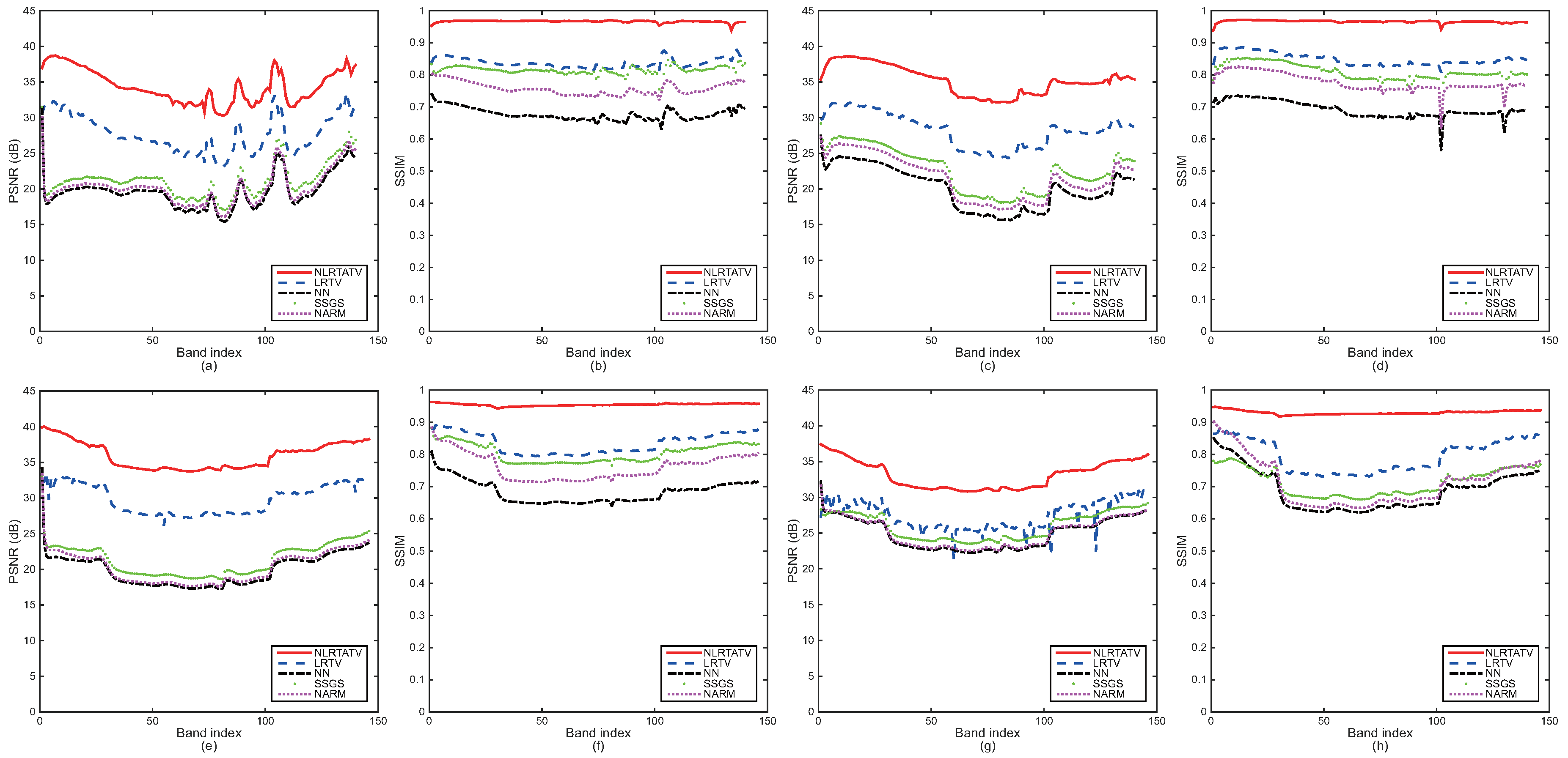
To provide more detailed quantitative comparison, we also show in Figure 2 and Figure 3 the PSNR and SSIM values of each band for all four of the cases listed in Table 1 and Table 2, respectively. As can be seen, the tensor methods including LRTV and the proposed NLRTATV can get much higher values of SSIM and PSNR than other ones for almost every band. In addition, NLRTATV can provide significantly improved reconstruction results over LRTV, especially for noise free cases. All of these show that the proposed NLRTATV can discover more intrinsic structures of HSIs than other competing ones, and thus it possesses a better reconstruction ability.
5.2. Visual Quality Comparison
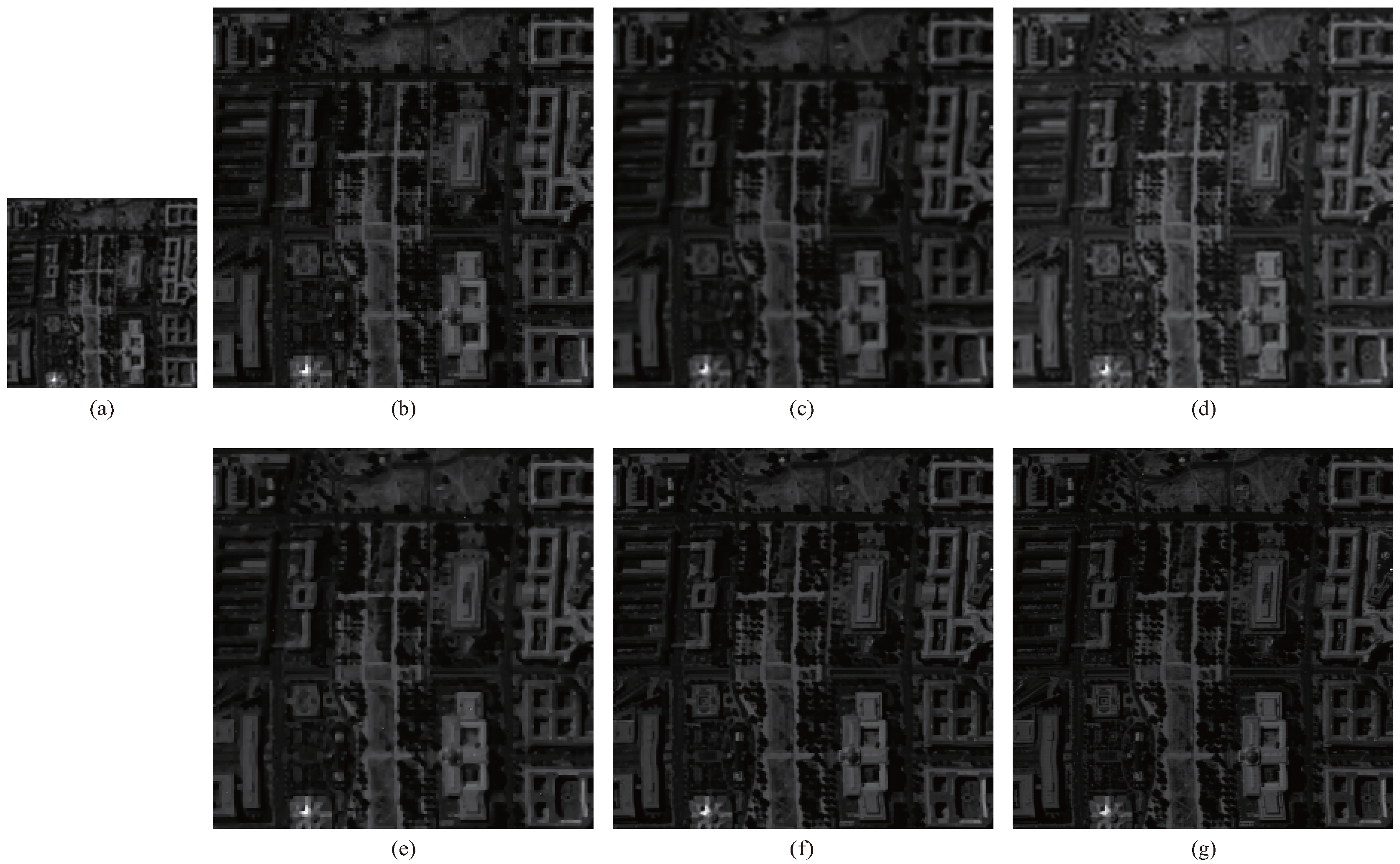
In terms of visual quality, one representative band of recovered HSIs in three typical cases obtained by all of the compared methods are shown in Figure 4, Figure 5 and Figure 6. It is evident that the images shown by (f) in the Figure 4, Figure 5 and Figure 6 recovered by our NLRTATV method preserve clearer and sharper edges compared with the other images shown by (b–e) in Figure 4, Figure 5 and Figure 6. One can zoom in on each figure for more visual comparison details.
5.3. Analysis of the Parameters
In the proposed NLRTATV model, there exist two regularization parameters and that need to be carefully identified. Thus, we provide some experimental analysis to show how we can choose them for practical use. (a) and (b) in Figure 7 describe the relationship between MPSNR and the regularization parameters and when NLRTATV performed on DC Mall data under noise free setting, respectively, with the other parameters fixed at optimal values. It can be observed that, as and vary in a wide range, the MPSNR value is rather stable and relatively stable correspondingly. Actually, we performed NLRTATV on several other experimental cases and found a similar behaviour as shown in Figure 7. Therefore, can be chosen as a value in and can be chosen as a value in in real implementation. For simplicity, in all the experiments conducted in this work, we set and as 0.3 and 0.04, respectively.
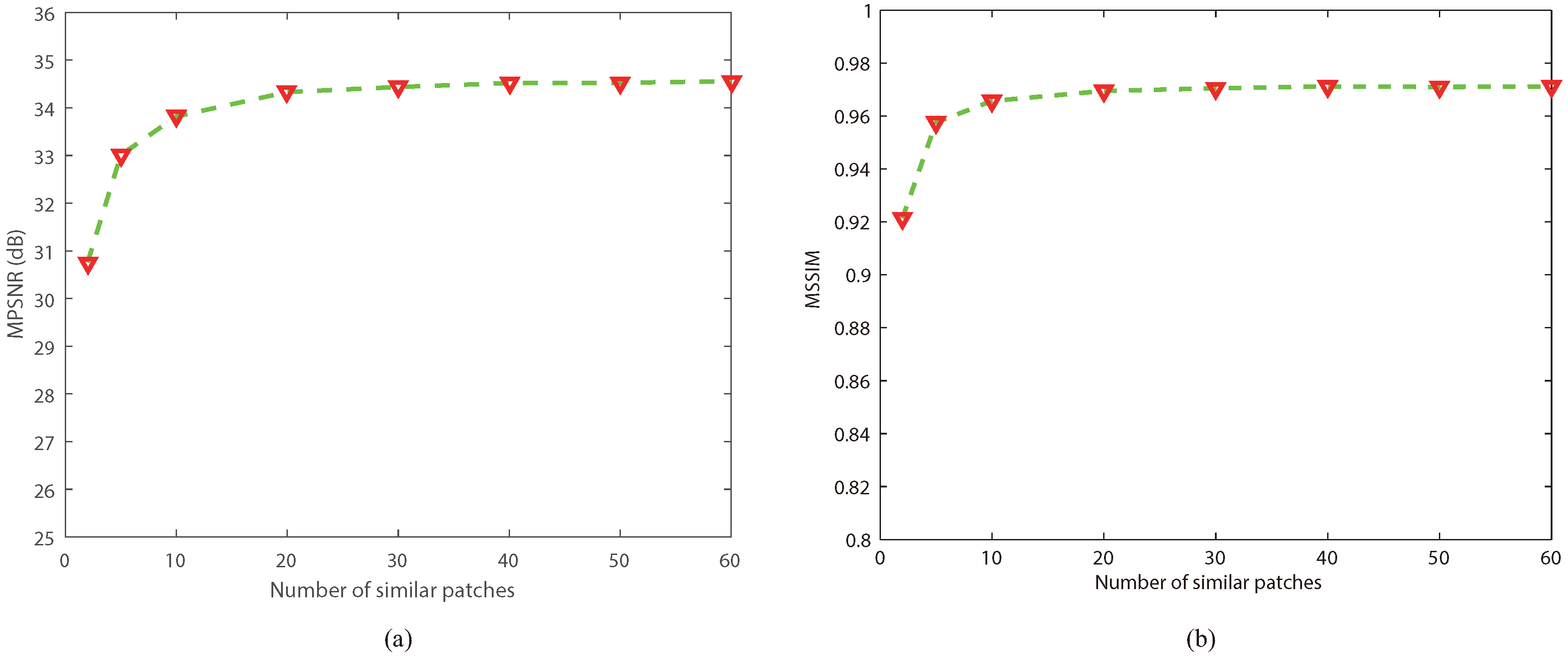
Since the nonlocal block matching operation is used in NLRTATV, the number of similar patches in each group is another important parameter that needs to be carefully considered. Figure 8 depicts the MPSNR and MSSIM gains versus the number of similar patches when NLRTATV performed on DC Mall data under a noise free setting. Here, we can observe that, as the number of similar patches increases to a value larger than 10, the curves of MPSNR and MSSIM both became stable. For simplicity, in all of the experiments, the number of similar patches was fixed to 30.
6. Conclusions
In this paper, we have proposed a novel method named NLRTATV for dealing with the problem of HSI super-resolution by using tensor structural modeling. The proposed method has considered the global correlation across spectral domain, the nonlocal self-similarity across spatial domain, and the local smooth structure across both spatial and spectral domains of the HSI cube by combining the low-rank tensor and 3D total variation regularizations. Extensive experimental study on three HSI datasets have demonstrated the superior performance of the proposed NLRTATV over several popular methods, which clearly shows the advantages of NLRTATV in exploring the intrinsic characteristics of the HSI cube.
Along this line, several desirable research directions can be conducted for future study. Firstly, though the proposed NLRTATV has only tested on the experiments with Gaussian blurring kernel, which is the situation in which no prior information on the blurring operator is known, a similar idea used in [18] could be incorporated into our model for tackling HSI super-resolution tasks with unknown blurring kernels. Secondly, it could be interesting to extend the deep learning ideas of [44] and [45] to design a deep tensor architecture to learn the more intrinsic characteristics of the HSI cube, and, as a result, to provide much better super-resolution reconstruction results. Thirdly, the problem of hyperspectral and multispectral data fusion has received much attention in recent years. It would be also interesting to extend the presented tensor modeling technique for dealing with such problems, which could give more effective methods for enhancing the spatial resolution of hyperspectral data.
Acknowledgments
The authors thank Kaidong Wang for the help on paper revision. The authors are also grateful to the Editor and reviewers for their constructive comments that have helped improve this work significantly. This work was partially supported by the National Science Foundation of China (Grant Nos. 11501440, 61773367) and the China Postdoctoral Science Foundation (Grant No. 2017M610628). The authors also thank the support from the Youth Innovation Promotion Association CAS.
Author Contributions
All authors made significant contributions to this work. Yao Wang and Zhi Han conceived and designed the experiments; Xi’ai Chen and Shiying He performed the experiments; Yao Wang and Xi’ai Chen analyzed the data; Yao Wang and Zhi Han wrote the paper.
Conflicts of Interest
The authors declare no conflict of interest.
References
- Gu, Y.; Zheng, Y.; Zhang, J. Integration of spatial-spectral information for resolution enhancement in hyperspectral images. IEEE Trans. Geosci. Remote Sens. 2008, 46, 1347–1357. [Google Scholar]
- Akgun, T.; Altunbasak, Y.; Mersereau, R.M. Super-resolution reconstruction of hyperspectral images. IEEE Trans. Image Process. 2005, 14, 1860–1875. [Google Scholar] [CrossRef] [PubMed]
- Park, S.C.; Park, M.K.; Kang, M.G. Super-resolution image reconstruction: A technical overview. IEEE Signal Process. Mag. 2003, 20, 20–36. [Google Scholar]
- Farsiu, S.; Robinson, D.; Elad, M.; Milanfar, P. Advances and challenges in super-resolution. Int. J. Imaging Syst. Technol. 2006, 14, 47–57. [Google Scholar] [CrossRef]
- Tsai, R.Y.; Huang, T.S. Multi-frame image restoration and registration. Adv. Comput. Vis. Image Process. 1987, 1, 317–339. [Google Scholar]
- Kim, S.P.; Bose, N.K.; Valenzuela, H.M. Recursive reconstruction of high resolution image from noisy undersampled multiframes. IEEE Trans. Acoust. Speech Signal Process. 1990, 38, 1013–1027. [Google Scholar] [CrossRef]
- Rhee, S.; Kang, M.G. Discrete cosine transform based regularized high-resolution image reconstruction algorithm. Opt. Eng. 1999, 38, 1348–1356. [Google Scholar] [CrossRef]
- Chan, R.H.; Chan, T.F.; Shen, L.; Shen, Z. Wavelet algorithms for high-resolution image reconstruction. SIAM J. Sci. Comput. 2003, 24, 1408–1432. [Google Scholar] [CrossRef]
- Ur, H.; Gross, D. Improved resolution from sub-pixel shifted pictures. CVGIP Graph. Models Image Process. 1992, 54, 181–186. [Google Scholar] [CrossRef]
- Irani, M.; Peleg, S. Improving resolution by image registration. CVGIP Graph. Models Image Process. 1991, 53, 231–239. [Google Scholar] [CrossRef]
- Yokoya, N.; Yairi, T.; Iwasaki, A. Coupled nonnegative matrix factorization unmixing for hyperspectral and multispectral data fusion. IEEE Trans. Geosci. Remote Sens. 2012, 50, 528–537. [Google Scholar] [CrossRef]
- Akhtar, N.; Shafait, F.; Mian, A. Sparse spatio-spectral representation for hyperspectral image super-resolution. In Proceedings of the ECCV 2014 European Conference on Computer Vision, Zürich, Switzerland, 6–12 September 2014; pp. 63–78. [Google Scholar]
- Loncan, L.; de Almeida, L.B.; Bioucas-Dias, J.M.; Briottet, X.; Chanussot, J.; Dobigeon, N.; Fabre, S.; Liao, W.; Licciardi, G.A.; Simoes, M.; et al. Hyperspectral pansharpening: A review. IEEE Geosci. Remote Mag. 2015, 3, 27–46. [Google Scholar] [CrossRef]
- Yang, J.; Li, Y.; Chan, J.C.W.; Shen, Q. Image Fusion for Spatial Enhancement of Hyperspectral Image via Pixel Group Based Non-Local Sparse Representation. Remote Sens. 2017, 9, 53. [Google Scholar] [CrossRef]
- Guo, Z.; Wittman, T.; Osher, S. L1 unmixing and its application to hyperspectral image enhancement. In Proceedings of the SPIE Conference on Algorithms and Technologies for Multispectral, Hyperspectral, and Ultraspectral Imagery XV, Orlando, FL, USA, 13–17 April 2009. [Google Scholar]
- Zhao, Y.; Yang, J.; Zhang, Q.; Song, L.; Cheng, Y.; Pan, Q. Hyperspectral imagery super-resolution by sparse representation and spectral regularization. EURASIP J. Adv. Signal Process. 2011, 2011, 87. [Google Scholar] [CrossRef]
- Zhang, H.; Zhang, L.; Shen, H. A super-resolution reconstruction algorithm for hyperspectral images. Signal Process. 2012, 92, 2082–2096. [Google Scholar] [CrossRef]
- Huang, H.; Christodoulou, A.; Sun, W. Super-resolution hyperspectral imaging with unknown blurring by low-rank and group-sparse modeling. In Proceedings of the ICIP 2014 International Conference on Image Processing, Paris, France, 27–30 October 2014; pp. 2155–2159. [Google Scholar]
- Li, J.; Yuan, Q.; Shen, H.; Meng, X.; Zhang, L. Hyperspectral image super-resolution by spectral mixture analysis and spatial–spectral group sparsity. IEEE Geosci. Remote Sens. Lett. 2016, 13, 1250–1254. [Google Scholar] [CrossRef]
- Yang, J.; Wright, J.; Huang, T.S.; Ma, Y. Image super-resolution via sparse representation. IEEE Trans. Image Process. 2008, 19, 2861–2873. [Google Scholar] [CrossRef] [PubMed]
- Dong, W.; Zhang, L.; Lukac, R.; Shi, G. Sparse Representation based Image Interpolation with nonlocal autoregressive modeling. IEEE Trans. Image Process. 2013, 22, 1382–1394. [Google Scholar] [CrossRef] [PubMed]
- He, S.; Zhou, H.; Wang, Y.; Cao, W.; Han, Z. Super-resolution reconstruction of hyperspectral images via low rank tensor modeling and total variation regularization. In Proceedings of the 2016 IEEE International Geoscience and Remote Sensing Symposium (IGARSS), Beijing, China, 10–15 July 2016; pp. 6962–6965. [Google Scholar]
- Shi, F.; Cheng, J.; Wang, L.; Yap, P.T.; Shen, D. LRTV: MR image super-resolution with low-rank and total variation regularizations. IEEE Trans. Med. Imaging 2015, 34, 2459–2466. [Google Scholar] [CrossRef] [PubMed]
- Kolda, T.G.; Bader, B.W. Tensor Decompositions and Applications. SIAM Rev. 2009, 51, 455–500. [Google Scholar] [CrossRef]
- Cao, W.; Wang, Y.; Yang, C.; Chang, X.; Han, Z.; Xu, Z. Folded-concave penalization approaches to tensor completion. Neurocomputing 2015, 152, 261–273. [Google Scholar] [CrossRef]
- Fan, J.; Xue, L.; Zou, H. Strong oracle optimality of folded concave penalized estimation. Ann. Stat. 2014, 41, 828–849. [Google Scholar] [CrossRef]
- Liu, J.; Musialski, P.; Wonka, P.; Ye, J. Tensor Completion for Estimating Missing Values in Visual Data. IEEE Trans. Pattern Anal. Mach. Intell. 2013, 35, 208–220. [Google Scholar] [CrossRef] [PubMed]
- He, W.; Zhang, H.; Zhang, L.; Shen, H. Total-variation-regularized low-rank matrix factorization for hyperspectral image restoration. IEEE Trans. Geosci. Remote Sens. 2016, 54, 178–188. [Google Scholar] [CrossRef]
- Wu, Z.; Wang, Q.; Wu, Z.; Shen, Y. Total variation-regularized weighted nuclear norm minimization for hyperspectral image mixed denoising. J. Electron. Imaging 2016, 25, 013037. [Google Scholar] [CrossRef]
- Mairal, J.; Bach, F.; Ponce, J.; Sapiro, G.; Zisserman, A. Non-local sparse models for image restoration. In Proceedings of the 2009 IEEE 12th International Conference on Computer Vision, Kyoto, Japan, 27 September–4 October 2009; pp. 2272–2279. [Google Scholar]
- Dong, W.; Shi, G.; Li, X. Nonlocal image restoration with bilateral variance estimation: A low-rank approach. IEEE Trans. Image Process. 2013, 22, 700–711. [Google Scholar] [CrossRef] [PubMed]
- Peng, Y.; Meng, D.; Xu, Z.; Gao, C.; Yang, Y.; Zhang, B. Decomposable nonlocal tensor dictionary learning for multispectral image denoising. In Proceedings of the IEEE Conference on Computer Vision and Pattern Recognition, Columbus, OH, USA, 24–27 June 2014; pp. 2949–2956. [Google Scholar]
- Cao, W.; Wang, Y.; Sun, J.; Meng, D.; Yang, C.; Cichocki, A.; Xu, Z. Total Variation Regularized Tensor RPCA for Background Subtraction From Compressive Measurements. IEEE Trans. Image Process. 2016, 25, 4075–4090. [Google Scholar] [CrossRef] [PubMed]
- Dabov, K.; Foi, A.; Katkovnik, V.; Egiazarian, K. Image denoising by sparse 3-D transform-domain collaborative filtering. IEEE Trans. Image Process. 2007, 16, 2080–2095. [Google Scholar] [CrossRef] [PubMed]
- Bunea, F.; She, Y.; Wegkamp, M. Optimal selection of reduced rank estimators of high-dimensional matrices. Ann. Stat. 2011, 52, 1282–1309. [Google Scholar] [CrossRef]
- Boyd, S.; Parikh, N.; Chu, E.; Peleato, B.; Eckstein, J. Distributed optimization and statistical learning via the alternating direction method of multipliers. Found. Trends Mach. Learn. 2011, 3, 1–122. [Google Scholar] [CrossRef]
- Airborne Visible/Infrared Imaging Spectrometer (AVIRIS) Moffett Field Data Set. Available online: https://aviris.jpl.nasa.gov/data/image_cube.html (accessed on 19 July 2017).
- Hyperspectral Digital Imagery Collection Experiment (HYDICE) Urban Data Set. Available online: http://www.tec.army.mil/hypercube (accessed on 19 July 2017).
- HYDICE Washington DC Mall Data Set. Available online: https://engineering.purdue.edu/~biehl/MultiSpec/hyperspectral.html (accessed on 19 July 2017).
- Yuan, Q.; Zhang, L.; Shen, H. Hyperspectral image denoising employing a spectral—Spatial adaptive total variation model. IEEE Trans. Geosci. Remote Sens. 2012, 50, 3660–3677. [Google Scholar] [CrossRef]
- Keshava, N. Distance metrics and band selection in hyperspectral processing with applications to material identification and spectral libraries. IEEE Trans. Geosci. Remote Sens. 2004, 42, 1552–1565. [Google Scholar] [CrossRef]
- Peak Signal-to-Noise Ratio. Available online: https://en.wikipedia.org/wiki/Peak_signal-to-noise_ratio. (accessed on 19 November 2017).
- Wang, Z.; Bovik, A.C.; Sheikh, H.R.; Simoncelli, E.P. Image quality assessment: From error visibility to structural similarity. IEEE Trans. Image Process. 2004, 13, 600–612. [Google Scholar] [CrossRef] [PubMed]
- Gregor, K.; LeCun, Y. Learning fast approximations of sparse coding. In Proceedings of the 27th International Conference on Machine Learning, Haifa, Israel, 21–24 June 2010; pp. 399–406. [Google Scholar]
- Sprechmann, P.; Bronstein, A.M.; Sapiro, G. Learning efficient sparse and low rank models. IEEE Trans. Pattern Anal. Mach. Intell. 2015, 37, 1821–1833. [Google Scholar] [CrossRef] [PubMed]
Figure 1.
The framework of our proposed procedure.
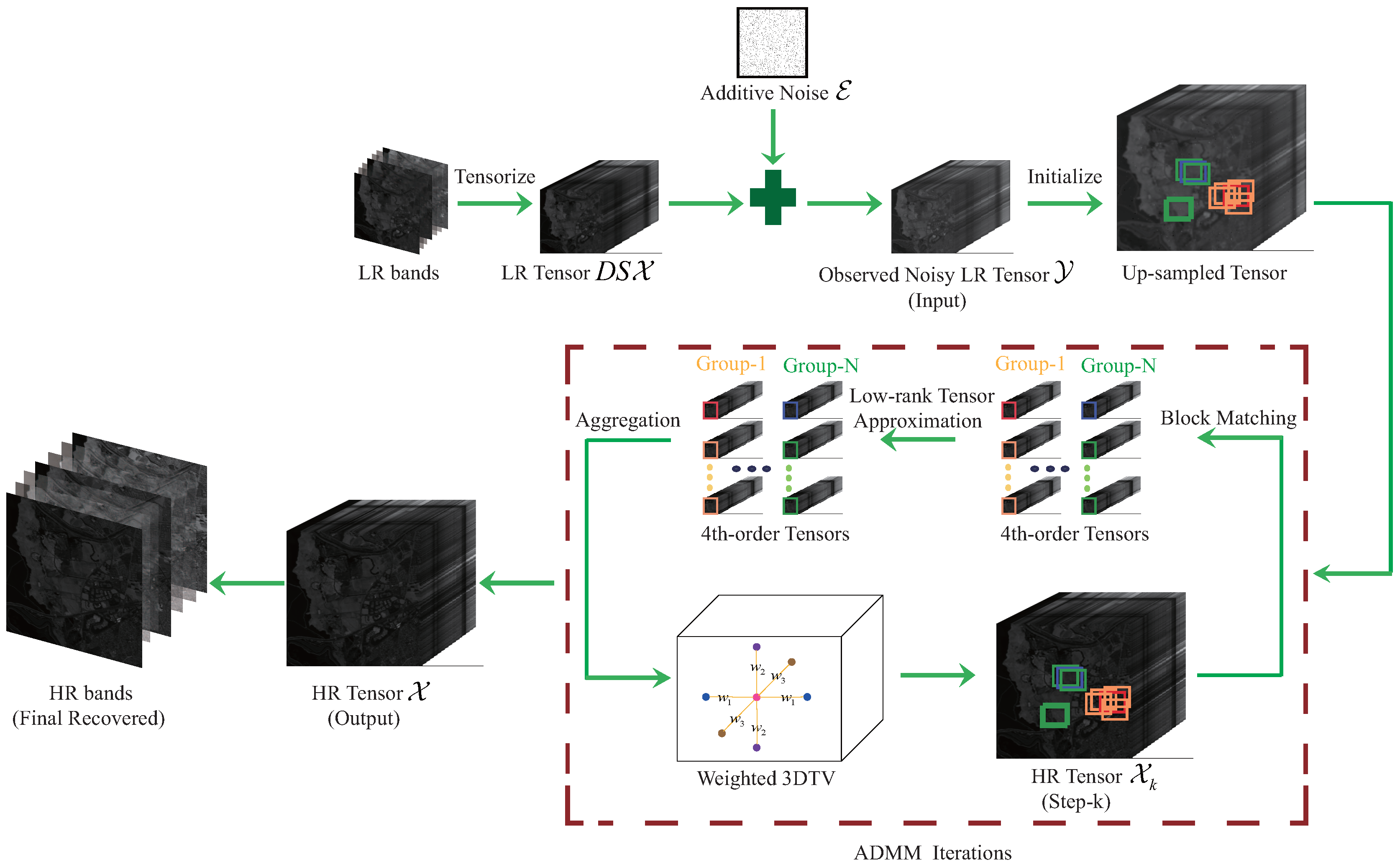
Figure 2.
Detailed quantitative evaluation of different methods for each band under noise free setting: (a,b) DC Mall (factor 2), (c,d) Urban (factor 2), (e,f) Moffett Field (factor 2), (g,h) Moffett Field (factor 3).
Figure 2.
Detailed quantitative evaluation of different methods for each band under noise free setting: (a,b) DC Mall (factor 2), (c,d) Urban (factor 2), (e,f) Moffett Field (factor 2), (g,h) Moffett Field (factor 3).

Figure 3.
Detailed quantitative evaluation of different methods for each band under noisy setting with : (a,b) DC Mall (factor 2), (c,d) Urban (factor 2), (e,f) Moffett Field (factor 2), (g,h) Moffett Field (factor 3).
Figure 3.
Detailed quantitative evaluation of different methods for each band under noisy setting with : (a,b) DC Mall (factor 2), (c,d) Urban (factor 2), (e,f) Moffett Field (factor 2), (g,h) Moffett Field (factor 3).
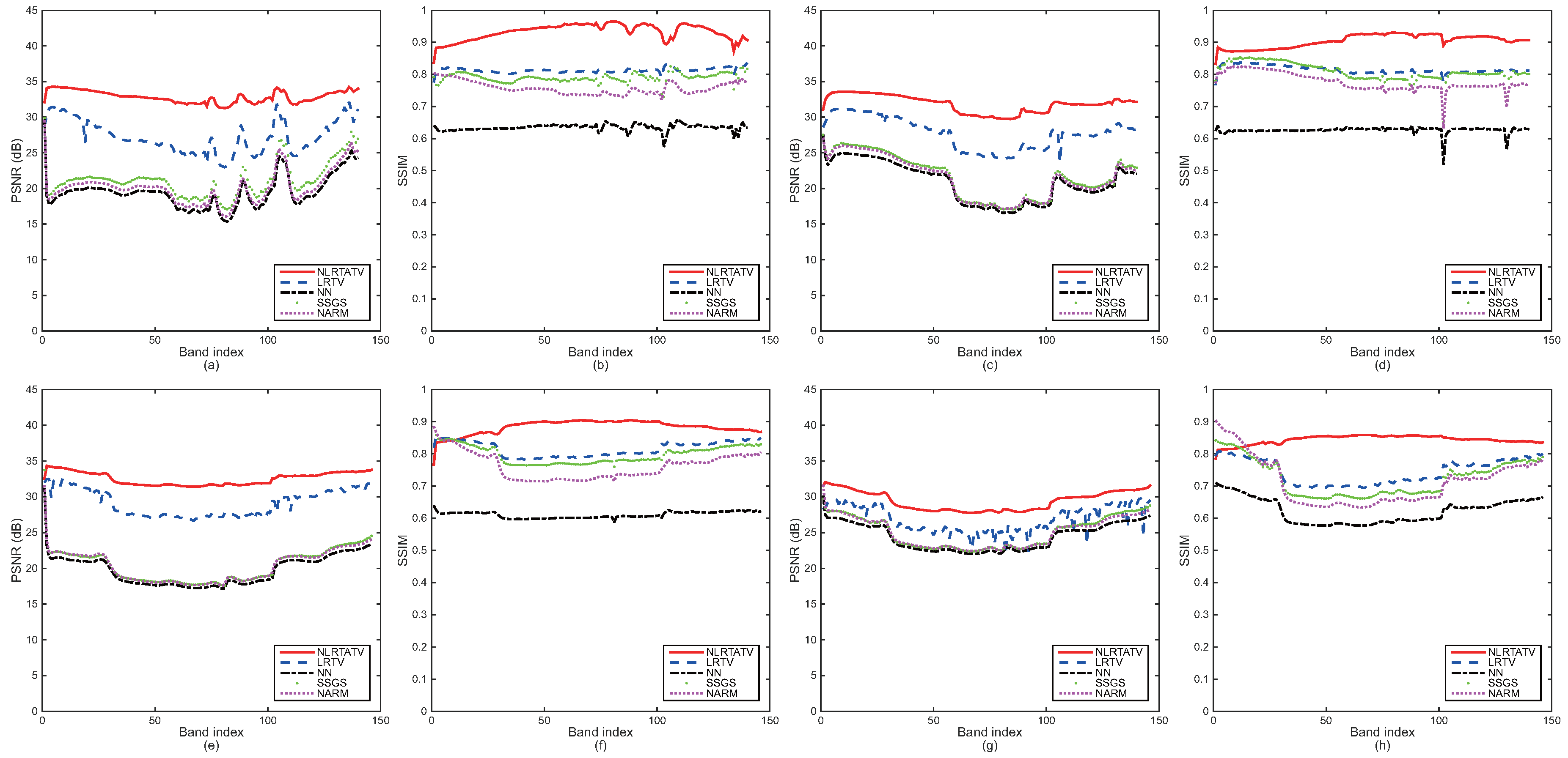
Figure 4.
Reconstruction results on band 137 of noise free DC Mall data with downsampling factor 2: (a) LR band with downsampling factor 2, (b) NN, (c) NARM, (d) SSGS, (e) LRTV, (f) NLRTATV, (g) original band.
Figure 4.
Reconstruction results on band 137 of noise free DC Mall data with downsampling factor 2: (a) LR band with downsampling factor 2, (b) NN, (c) NARM, (d) SSGS, (e) LRTV, (f) NLRTATV, (g) original band.

Figure 5.
Reconstruction results on band 34 of noise free Moffet Field data with downsampling factor 2: (a) LR band with downsampling factor 2, (b) NN, (c) NARM, (d) SSGS, (e) LRTV, (f) NLRTATV, (g) original band.
Figure 5.
Reconstruction results on band 34 of noise free Moffet Field data with downsampling factor 2: (a) LR band with downsampling factor 2, (b) NN, (c) NARM, (d) SSGS, (e) LRTV, (f) NLRTATV, (g) original band.
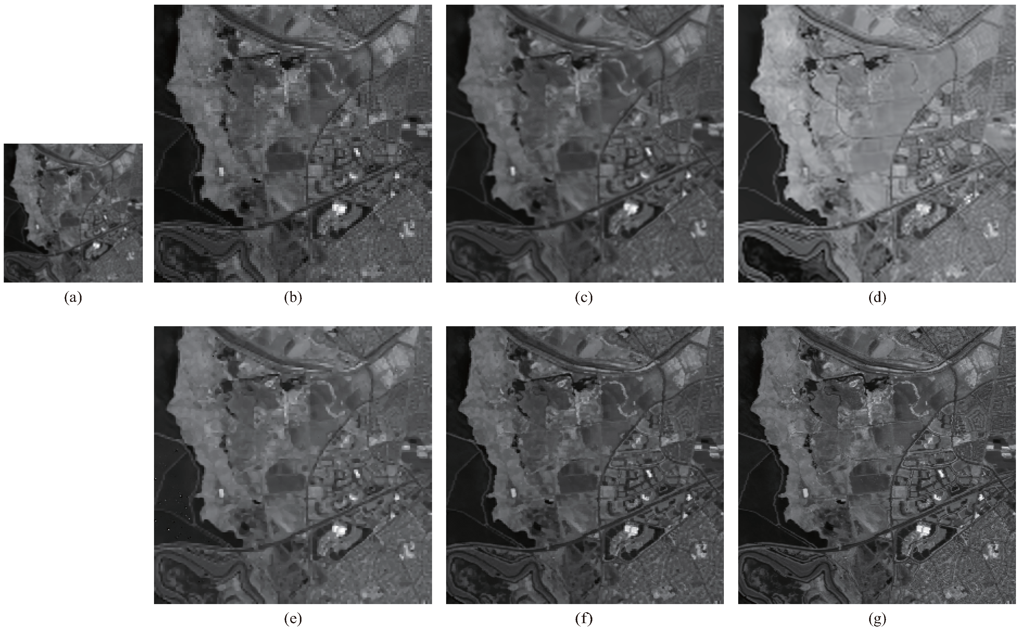
Figure 6.
Reconstruction results on band 56 of noisy Urban data with downsampling factor 2: (a) LR band with downsampling factor 2, (b) NN, (c) NARM, (d) SSGS, (e) LRTV, (f) NLRTATV, (g) original band.
Figure 6.
Reconstruction results on band 56 of noisy Urban data with downsampling factor 2: (a) LR band with downsampling factor 2, (b) NN, (c) NARM, (d) SSGS, (e) LRTV, (f) NLRTATV, (g) original band.
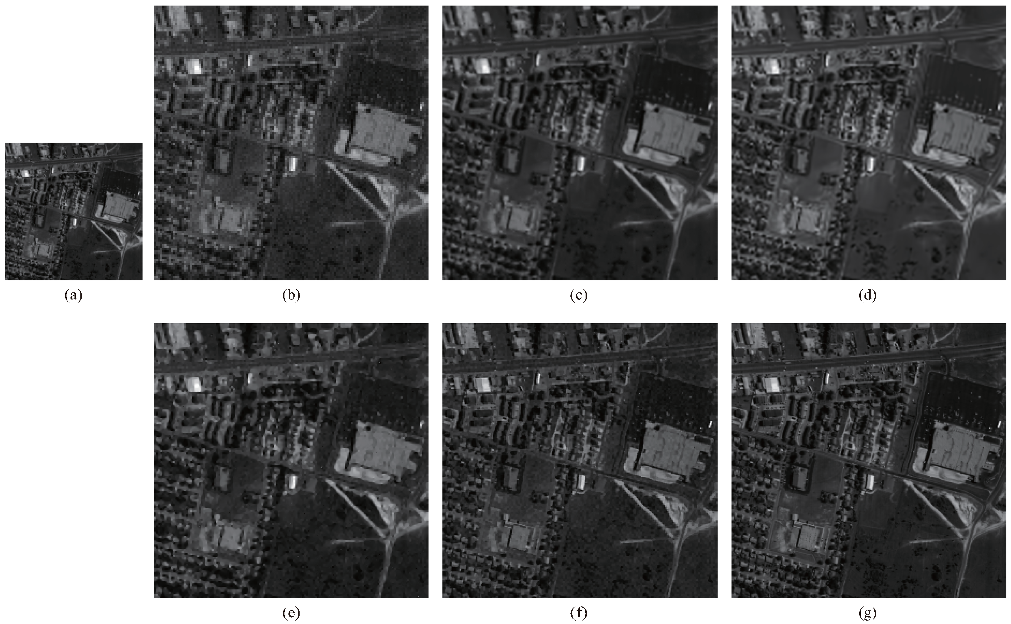
Figure 7.
Sensitivity analysis of two regularization parameters: (a) the MPSNR value versus ; (b) the MPSNR value versus .
Figure 7.
Sensitivity analysis of two regularization parameters: (a) the MPSNR value versus ; (b) the MPSNR value versus .
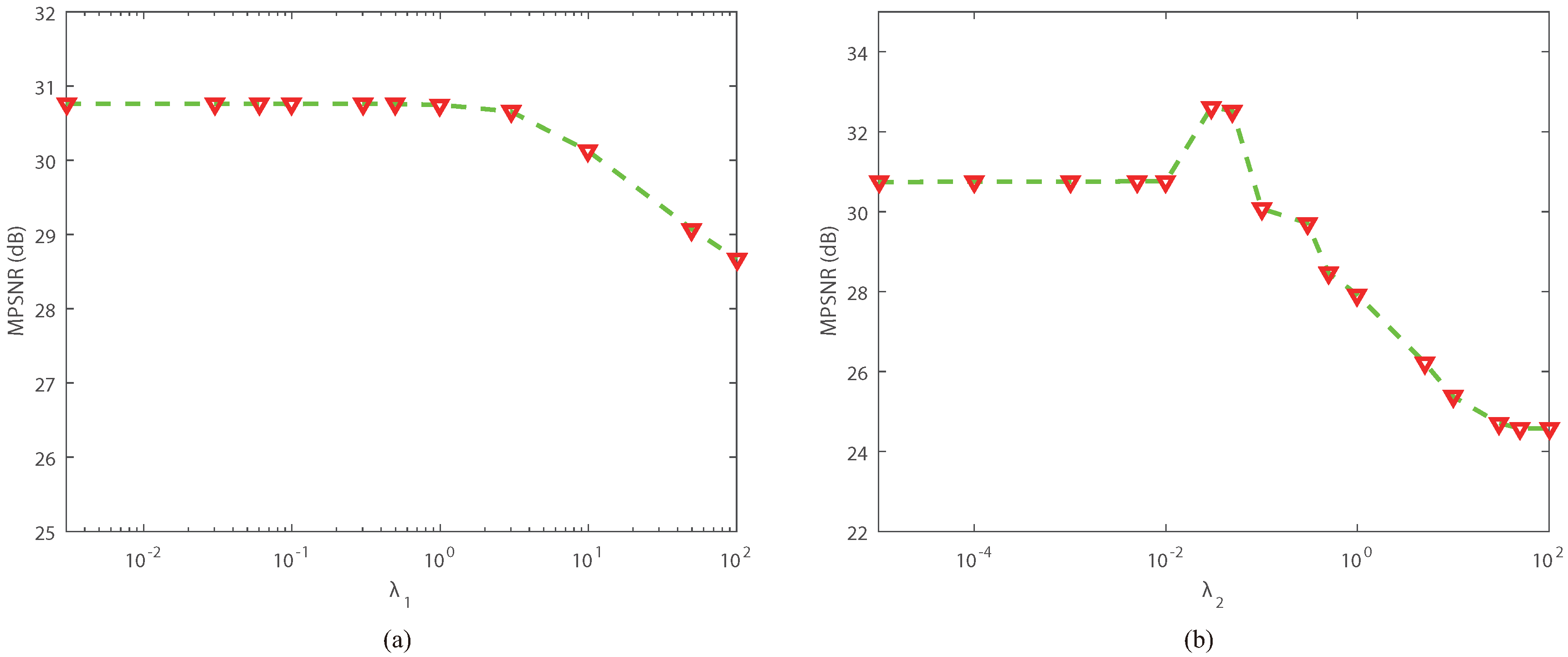
Figure 8.
Sensitivity analysis of the number of similar patches: (a) change in the MPSNR value; (b) change in the MSSIM value.
Figure 8.
Sensitivity analysis of the number of similar patches: (a) change in the MPSNR value; (b) change in the MSSIM value.


Table 1.
Super-resolution reconstruction results by different methods under noise free setting.
| NN | NARM | SSGS | LRTV | NLRTATV | ||
|---|---|---|---|---|---|---|
| MPSNR (dB) | 19.6357 | 20.1774 | 21.2733 | 27.7744 | 34.3935 | |
| DC Mall (factor 2) | MSSIM | 0.6771 | 0.7575 | 0.8142 | 0.8380 | 0.9665 |
| SAM (rad) | 0.0998 | 0.0913 | 0.0875 | 0.0805 | 0.0487 | |
| MPSNR (dB) | 20.1281 | 21.5613 | 22.7087 | 28.2954 | 35.2754 | |
| Urban (factor 2) | MSSIM | 0.6924 | 0.7770 | 0.8092 | 0.8485 | 0.9663 |
| SAM (rad) | 0.0971 | 0.0837 | 0.0789 | 0.0710 | 0.0470 | |
| MPSNR (dB) | 19.9535 | 20.3799 | 21.4042 | 29.8499 | 35.9816 | |
| Moffett Field (factor 2) | MSSIM | 0.6836 | 0.7621 | 0.8042 | 0.8349 | 0.9545 |
| SAM (rad) | 0.0958 | 0.0820 | 0.0754 | 0.0630 | 0.0365 | |
| MPSNR (dB) | 24.9190 | 25.1116 | 26.0086 | 27.4270 | 33.1308 | |
| Moffett Field (factor 3) | MSSIM | 0.6888 | 0.7130 | 0.7139 | 0.7955 | 0.9301 |
| SAM (rad) | 0.0963 | 0.0915 | 0.0901 | 0.0810 | 0.0476 |
Table 2.
Super-resolution reconstruction results by different methods under noisy setting ().
| NN | NARM | SSGS | LRTV | NLRTATV | ||
|---|---|---|---|---|---|---|
| MPSNR (dB) | 19.4578 | 20.1558 | 21.2191 | 27.2824 | 32.8701 | |
| DC Mall (factor 2) | MSSIM | 0.6346 | 0.7575 | 0.7901 | 0.8126 | 0.9329 |
| SAM (rad) | 0.1034 | 0.0913 | 0.0889 | 0.0845 | 0.0473 | |
| MPSNR (dB) | 20.8761 | 21.4544 | 21.6906 | 27.7523 | 31.8675 | |
| Urban (factor 2) | MSSIM | 0.6263 | 0.7770 | 0.8090 | 0.8148 | 0.9042 |
| SAM (rad) | 0.0928 | 0.0897 | 0.0835 | 0.0745 | 0.0628 | |
| MPSNR (dB) | 19.7640 | 20.3251 | 20.4034 | 29.1580 | 32.5487 | |
| Moffett Field (factor 2) | MSSIM | 0.6107 | 0.7621 | 0.7982 | 0.8158 | 0.8834 |
| SAM (rad) | 0.0905 | 0.0720 | 0.0695 | 0.0635 | 0.0470 | |
| MPSNR (dB) | 24.4130 | 25.0118 | 25.0782 | 26.8280 | 29.4416 | |
| Moffett Field (factor 3) | MSSIM | 0.6223 | 0.7130 | 0.7247 | 0.7458 | 0.8441 |
| SAM (rad) | 0.0929 | 0.0915 | 0.0864 | 0.0839 | 0.0660 |
© 2017 by the authors. Licensee MDPI, Basel, Switzerland. This article is an open access article distributed under the terms and conditions of the Creative Commons Attribution (CC BY) license (http://creativecommons.org/licenses/by/4.0/).
Share and Cite
MDPI and ACS Style
Wang, Y.; Chen, X.; Han, Z.; He, S. Hyperspectral Image Super-Resolution via Nonlocal Low-Rank Tensor Approximation and Total Variation Regularization. Remote Sens. 2017, 9, 1286. https://doi.org/10.3390/rs9121286
AMA Style
Wang Y, Chen X, Han Z, He S. Hyperspectral Image Super-Resolution via Nonlocal Low-Rank Tensor Approximation and Total Variation Regularization. Remote Sensing. 2017; 9(12):1286. https://doi.org/10.3390/rs9121286
Chicago/Turabian StyleWang, Yao, Xi’ai Chen, Zhi Han, and Shiying He. 2017. "Hyperspectral Image Super-Resolution via Nonlocal Low-Rank Tensor Approximation and Total Variation Regularization" Remote Sensing 9, no. 12: 1286. https://doi.org/10.3390/rs9121286
Note that from the first issue of 2016, this journal uses article numbers instead of page numbers. See further details here.