Uncertainty of Remote Sensing Data in Monitoring Vegetation Phenology: A Comparison of MODIS C5 and C6 Vegetation Index Products on the Tibetan Plateau

1
State Key Laboratory of Earth Surface Processes and Resource Ecology, Beijing Normal University, Beijing 100875, China
2
Joint Center for Global Change Studies (JCGCS), Beijing 100875, China
3
Beijing Engineering Research Center for Global Land Remote Sensing Products, Institute of Remote Sensing Science and Engineering, Faculty of Geographical Science, Beijing Normal University, Beijing 100875, China
*
Authors to whom correspondence should be addressed.
†
These authors contributed equally to this work.
Remote Sens. 2017, 9(12), 1288; https://doi.org/10.3390/rs9121288
Submission received: 29 September 2017
/
Revised: 4 December 2017
/
Accepted: 7 December 2017
/
Published: 11 December 2017
(This article belongs to the Special Issue Advances in Quantitative Remote Sensing in China – In Memory of Prof. Xiaowen Li)
Abstract
:Vegetation phenology is considered a sensitive indicator of climate change, which controls carbon, nitrogen, and water cycles within terrestrial ecosystems. The Moderate Resolution Imaging Spectroradiometer (MODIS) Normalized Difference Vegetation Index (NDVI) is an important moderate resolution remote sensing data for monitoring vegetation phenology. However, Terra MODIS Collection 5 (C5) vegetation index products were identified to be affected by sensor degradation, which has been addressed in the recently released MODIS Collection 6 (C6) vegetation index products. In order to compare the difference between MODIS C5 and C6 NDVI in monitoring vegetation phenology, the start and end of growing season (SOS and EOS) of the alpine grassland on the Tibetan Plateau (TP) were extracted using four common methods. Then, the C5 and C6 NDVI-derived SOS (SOSC5 and SOSC6) and EOS (EOSC5 and EOSC6) were compared with ground-observed phenology data. Results showed that the multi-year average growing season NDVIs of C6 were lower than those of C5 in most areas, while the inter-annual variation patterns of regional average SOSC5 and SOSC6 (EOSC5 and EOSC6) were consistent. However, large spatial differences in phenological trends were found between C5 and C6 NDVI products. From C5 to C6, pixels with a SOS (EOS) trend shifting from significant to insignificant or from insignificant to significant accounted for at least 14.58% (9.07%) of the total pixels. SOSC5 was more consistent than SOSC6 with the ground-observed green-up dates. C5 NDVI may be more appropriate for monitoring SOS than C6 NDVI in the study region, but more ground-observed phenology records are needed to confirm it due to only four observational sites in this study. However, large differences and poor correlations existed between EOSC5 (EOSC6) and the ground-observed beginning of leaf coloring. To further evaluate the uncertainty of MODIS C5 and C6 NDVI in monitoring vegetation phenology, higher resolution near-surface remote sensing data and corresponding validation methods should be applied.
1. Introduction
Vegetation phenology dynamics can reflect the response of terrestrial ecosystem to climate change and play an important role in adjusting the cycling of carbon, nitrogen, and water [1,2,3]. Remote sensing data have been widely used to monitor vegetation phenology at large scales [4,5,6], because satellite-derived vegetation indices can measure vegetation canopy greenness and have the advantages of wide coverage, high revisiting frequency, and relatively low cost. The Normalized Difference Vegetation Index (NDVI) is one of the most commonly used vegetation indexes for monitoring vegetation phenology [7,8,9].
Moderate Resolution Imaging Spectroradiometer (MODIS) remote sensing data have been increasingly used for monitoring vegetation phenology. MODIS sensors aboard Terra and Aqua satellites have been in operation since 1999 and 2002, respectively, and can provide long-term remote sensing records of >10 years. However, the designed lifetimes of the sensors are only six years. In recent years, severe data problems were found to exist in MODIS Collection 5 (C5) ocean colors [10], aerosols [11], and NDVI products [12,13,14], mainly resulting from sensor degradation. Due to the increasing exposure of MODIS sensor to solar and cosmic radiation, severe degradation of Terra MODIS near-infrared, red and blue bands has been observed. The sensor degradation was the most pronounced in the Terra blue band and decreased with wavelength [12,13]. Though the blue band is not used directly to calculate NDVI, degradation of blue top-of-atmosphere reflectance over time will influence the calculation of surface reflectance in other spectral bands and NDVI [13,15,16]. Moreover, the sensor degradation was much faster for Terra than Aqua [13,17]. To remove the effects of sensor degradation, improved calibrated approaches were adopted to produce the recently released MODIS Collection 6 (C6) products [12,18]. When compared with C5, the C6 Level 1B data, including the top-of-atmosphere reflectance in the near-infrared, red and blue bands were calibrated [13]. In addition, the NDVI retrieval algorithms were also improved [19]. Unlike C5 NDVI, which uses daily reflectance data, C6 NDVI uses pre-composed (8-day) surface reflectance data that are atmospherically corrected with a modified compositing algorithm that aims to reduce the aerosol issues (minimizing the blue band) [17,19].
The differences between MODIS C5 and C6 NDVI have been evaluated in some previous studies (e.g., [17,20]). However, no study has conducted a comparative analysis of the performance of MODIS C5 and C6 NDVI in monitoring vegetation phenology. Given that MODIS C5 NDVI has been extensively used for monitoring vegetation phenology [21,22,23], it is necessary to analyze the difference between vegetation phenology derived from C5 and C6 NDVI and consequently investigate the uncertainty in monitoring vegetation phenology due to sensor degradation. Due to the fact that Terra data is more affected by the sensor degradation than Aqua data [13,17], this study focused on the Terra MODIS NDVI products.
Four common methods were adopted to identify the start and end of growing season (SOS and EOS) of the alpine grassland on the Tibetan Plateau (TP) based on Terra MODIS C5 and C6 NDVI. Then, a comparative analysis of vegetation phenology derived from the two NDVI products was conducted for each phenology extraction method. Meanwhile, the performances of vegetation phenology derived from C5 and C6 NDVI in capturing ground-observed phenology were also evaluated.
2. Data and Methods
2.1. Remote Sensing Data
The Terra MODIS 250 m 16-day composited NDVI (MOD13Q1) products originating from C5 and C6 during 2001–2015 were acquired from National Aeronautics and Space Administration (NASA) Earth Observing System Data and Information System (EOSDIS). To reduce the effect of cloud and Nadir Bidirectional Reflectance Distribution Function (BRDF), the composite of NDVI was performed by the Constrained View Angle-Maximum Value Composite (CV-MVC) algorithm. The pixel reliability (PR) layer from MOD13Q1 products was used to determine the pixel quality and calibrate NDVI time series. A PR value of 0 or 1 represents good pixel or marginal pixel in the NDVI time series. A PR value of 2 or 3 represents pixel covered by ice/snow or cloud, which should be corrected.
2.2. Ground-Observed Phenology Data
The ground-observed phenology data were collected from the nation-wide phenological observation network that was established by the China Meteorological Administration [24]. As Kobresia humilis is the dominant species in the alpine grassland on the TP, the ground-observed phenology data of K. humilis, including green-up (GU) and beginning of leaf coloring (BLC), were collected at Haiyan, Gande, Henan, and Qumarleb sites from 2001–2012 (Table 1).
2.3. Data Pre-Processing
The snow cover during the non-growing season on the TP will reduce NDVI values, resulting in retrieval errors for the phenology data. To reduce the effect of snow, snow-contaminated NDVI values (PR value equals 2) were replaced by the median value of the uncontaminated NDVI values (PR value equals 0 or 1) during the non-growing season (from November to the following March) for each pixel [25]. However, plenty of snow-contaminated pixels could not be flagged out by the PR values. Therefore, another way was applied to eliminate snow contamination. For each pixel, all of the NDVI values that were lower than the mean of the NDVI values during the non-growing season were replaced by the mean. After that, the Savitzky-Golay filter was used to reconstruct the NDVI time series to further remove cloud contamination [26]. In this study, all data were re-projected to the Albers conic equal area projection.
Only the vegetation phenology in the alpine grassland was analyzed in this study. To eliminate the effects of bare soil, sparse vegetation and evergreen forest, grass pixels were selected by the following criteria [25,27]: (1) the average NDVI for June–September should be greater than 0.1; (2) the annual maximum NDVI should exceed 0.15 and occur within July–September; (3) the average NDVI for July–September should be greater than 1.2 times of the average NDVI for November–March; and, (4) the average NDVI in winter (December–February) should be lower than 0.4.
2.4. Phenology Extraction Methods
Many methods have been used to extract vegetation phenology, but the vegetation phenology varied with extraction methods [28]. To avoid the effect of phenology extraction methods on the uncertainty analysis of remote sensing data in monitoring vegetation phenology, four commonly used methods were adopted to extract the SOS and EOS in the alpine grassland on the TP, i.e., the maximum curvature change method (MCC), dynamic threshold methods with a threshold of 0.2 and 0.5 (DT2 and DT5), and maximum slope method (MS).
2.4.1. MCC Method
A four-parameter logistic function [29] was employed to fit each increasing or decreasing section of a NDVI time series and then the daily NDVI values were derived from the fitted function, as shown below:
where t is the time (Julian day of year, DOY), y(t) is the NDVI value at time t, a and b are fitting parameters, c + d is the maximum NDVI value, and d is the initial background NDVI value [29]. Then, the curvature-change rate (CCR) of the fitted logistic curve was used to extract phenological dates, according to Equation (2) [29]:
where z = ea+b. SOS is defined as the DOY when CCR reaches its first local maximum value during the growth period, while EOS is defined as the DOY when CCR reaches its second minimum value during the senescence period.
2.4.2. DT2 and DT5 Methods
The phenological metrics were derived using the dynamic threshold method developed by White et al. [30]. In this method, the daily NDVI values were first generated using a linear interpolation approach from the original 16-day composites. SOS and EOS are defined as the DOY when the NDVI ratio reaches a certain threshold during the NDVI rising stage and decline stage, respectively. The NDVI ratio is defined as:
where NDVIt is the NDVI value at time t, NDVImax is the annual maximum NDVI value, NDVImin is the annual minimum NDVI value during the growth period for SOS or during the senescence period for EOS. In this study, the threshold was set to be 0.2 (0.5) for DT2 (DT5) method.
2.4.3. MS Method
In this method, SOS or EOS is defined as the DOY when NDVI begins to rapidly increase (SOS) or decrease (EOS) [31], which is identified based on the maximum absolute slope of the fitted NDVI curve in Equation (1) during the growth or senescence period.
2.5. Data Analysis Methods
The temporal change trends of regional average growing season (April–October) NDVI (GSNDVI) based on C5 and C6 products (GSNDVIC5 and GSNDVIC6) during 2001–2015 were calculated and compared. The change trends in the regional average GSNDVI were computed as the slope of the linear regression of the regional average GSNDVI against year. To analyze the spatial differences between C5 and C6 GSNDVIs, the pixel-by-pixel multi-year average values and linear trends were further calculated. With the same methods being used for comparing GSNDVI, the C5 and C6 NDVI-derived SOS (SOSC5 and SOSC6) as well as EOS (EOSC5 and EOSC6) identified by each phenology extraction method were further compared. Paired-samples t tests were conducted to compare the GSNDVI or phenological metrics between C5 and C6.
To validate the satellite-derived vegetation phenology, the average phenology of a 3 × 3 window centered at each site was extracted for comparison with the ground-observed phenology. The mean error (ME) and the mean absolute error (MAE) were used to estimate the difference between the satellite-derived phenology and the ground-observed phenology. They are calculated by the following formulas:
where P(rs)i and P(site)i are the satellite-derived phenology and the ground-observed phenology at sample i, respectively; n is the number of samples. In addition, the correlations between the satellite-derived phenology and the ground-observed phenology were also calculated to evaluate their consistency.
The statistical significance of all the regression coefficients and correlation coefficients was examined using the F-test. P values less than 0.05 were considered significant.
3. Results
3.1. Comparison Between GSNDVIC5 and GSNDVIC6
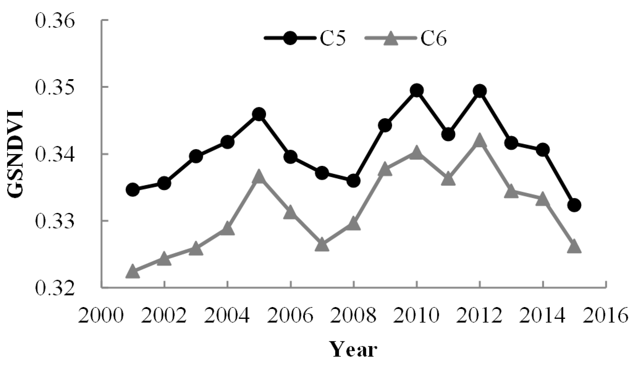
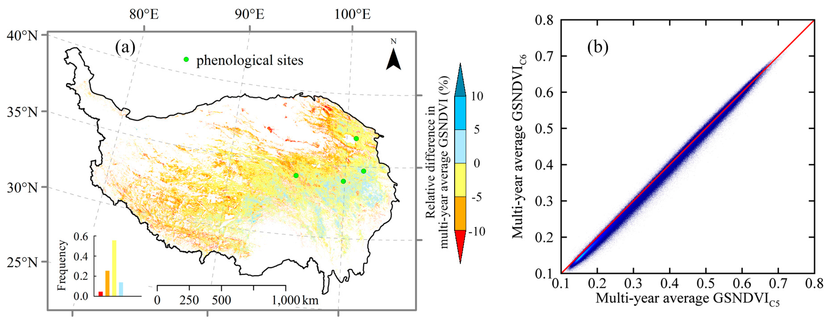
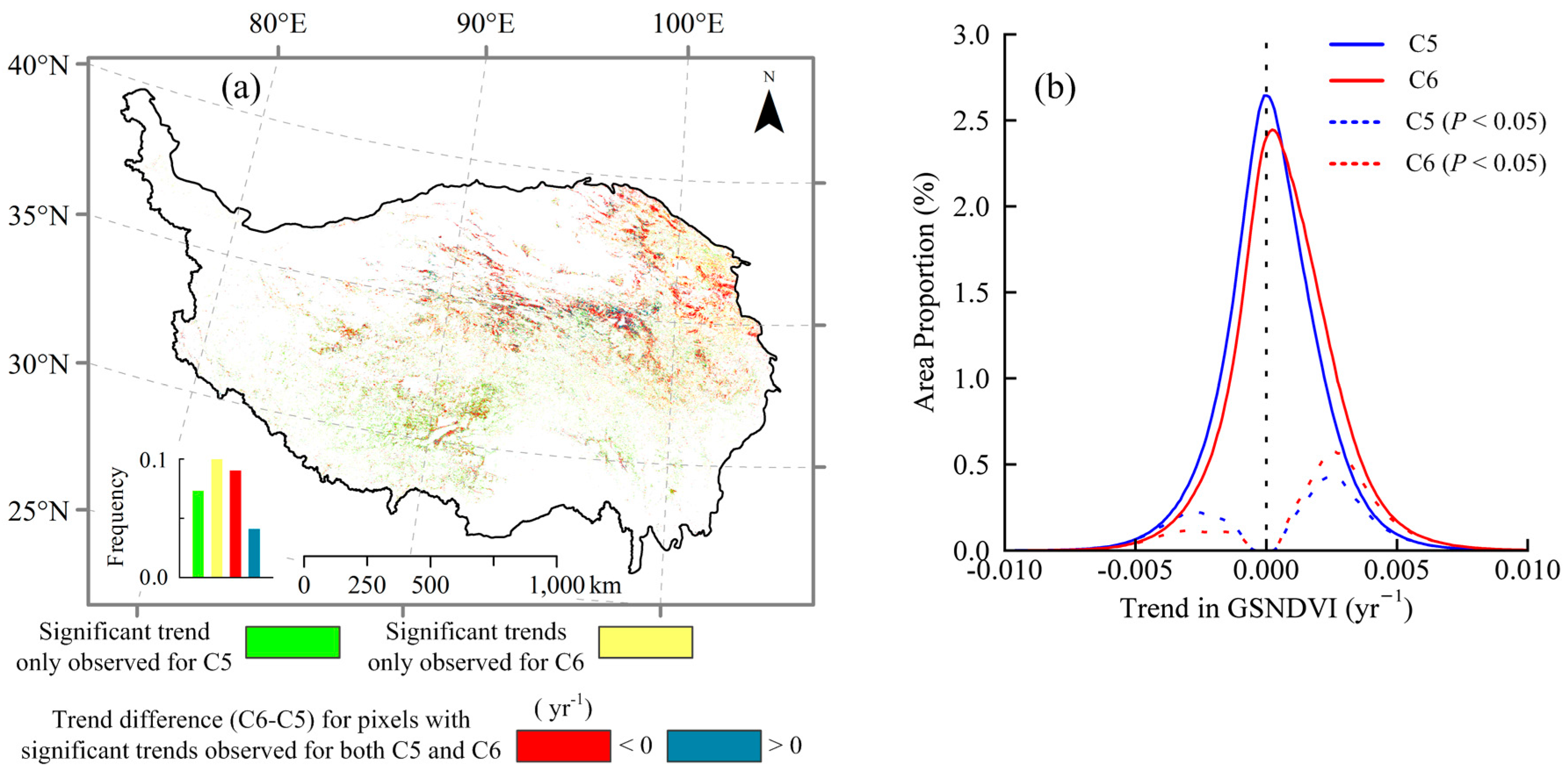
The regional average GSNDVIC6 was significantly (p < 0.001) lower than GSNDVIC5 for the alpine grassland on the TP (Figure 1). The annual regional average GSNDVI showed no obvious trend for C5 (p = 0.424), but a significant increasing trend for C6 (7.26 × 10⁻⁴ yr−1, p < 0.05) during 2001–2015 (Figure 1). At spatial scale, the multi-year average GSNDVIC6 was lower than GSNDVIC5 over 85.8% of the total pixels (Figure 2). The multi-year average GSNDVI decreased more than 5% from C5 to C6 over 30.13% of the pixels, while it increased more than 5% over only 0.12% of the pixels (Figure 2a). Moreover, large spatial differences in trends between GSNDVIC5 and GSNDVIC6 were found (Figure 3a). From GSNDVIC5 to GSNDVIC6, significant trends (p < 0.05) became insignificant over 7.33% of pixels, while insignificant trends became significant over 9.98% of pixels. With regard to the pixels where both GSNDVIC5 and GSNDVIC6 indicated significant trends, GSNDVI trend became more negative over 9.03% of pixels and more positive over 4.10% of pixels from C5 to C6. A significant (p < 0.001) difference between GSNDVIC5 and GSNDVIC6 trends was observed. The mean difference in GSNDVI trend (C6–C5) was −3.74 × 10⁻⁴ yr−1. Besides, GSNDVIC6 showed increasing trends over more area and decreasing trends over less area (65.3% increasing, 18.6% significantly increasing; 34.7% decreasing, 4.5% significantly decreasing) when compared with GSNDVIC5 (55.8% increasing, 12.9% significantly increasing; 44.2% decreasing, 7.6% significantly decreasing) (Figure 3b).
3.2. Temporal Differences in Regional Phenology
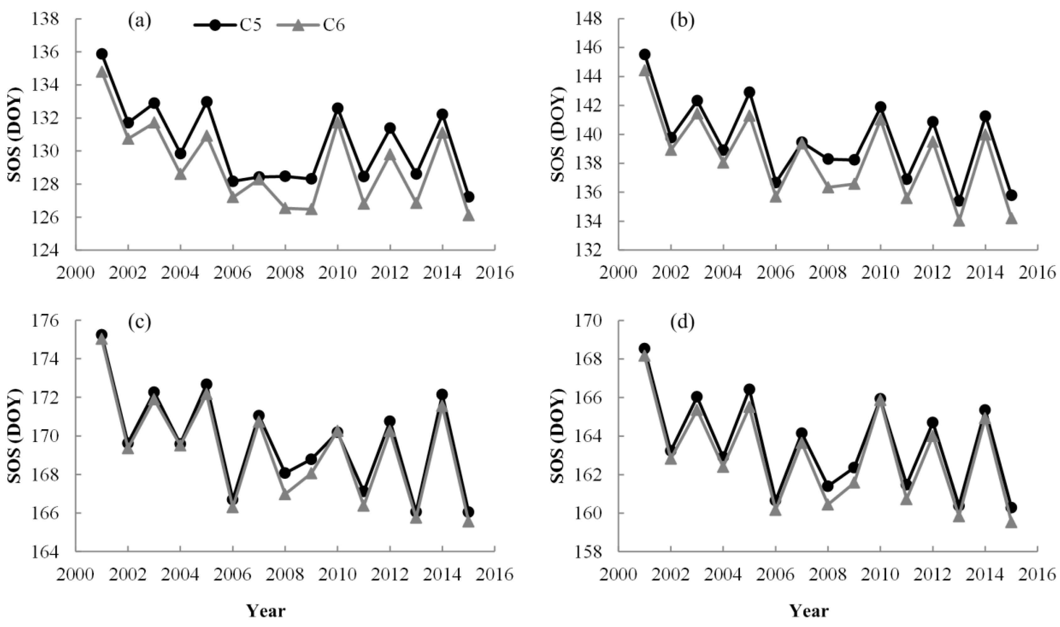
For each method, similar advancing trends were found between regional average SOSC5 and SOSC6 during 2001–2015, but the advancing trend of SOSC5 was slightly smaller than that of SOSC6 (Figure 4, Table 2). For each method, the multi-year average regional SOSC5 was significantly later than SOSC6 (p < 0.001), but the difference was only about one day (Table 2).
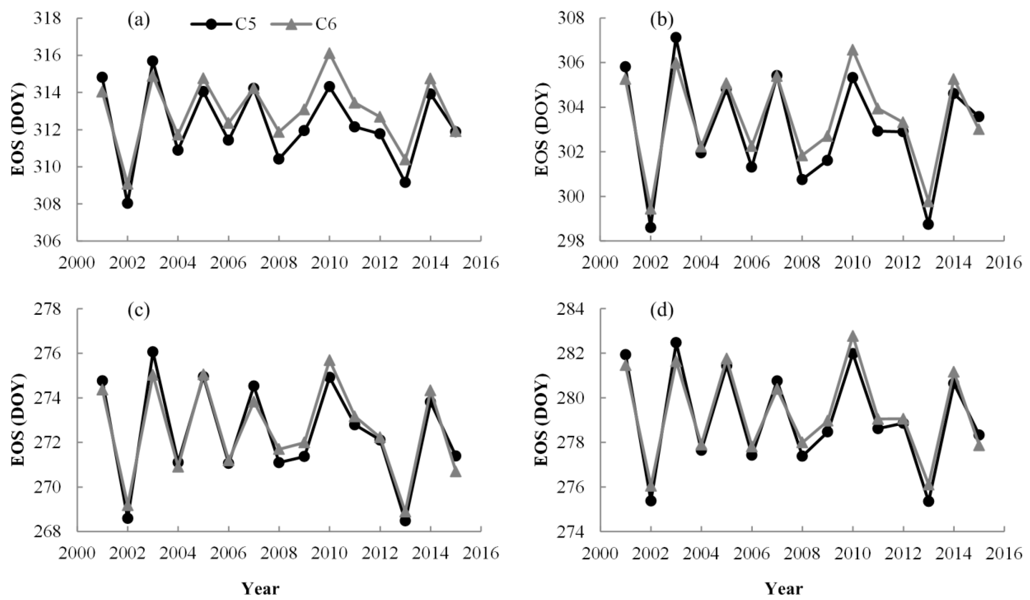
The regional average EOSC5 and EOSC6 also showed consistent inter-annual variations but no significant trends were found (Figure 5, Table 3). Different from SOS, the multi-year average regional EOSC5 was slightly earlier than EOSC6 for each method, with a difference of less than one day, but the difference was only significant (p < 0.05) for MCC and DT2 methods (Table 3).
3.3. Spatial Differences in Multi-Year Average Phenology
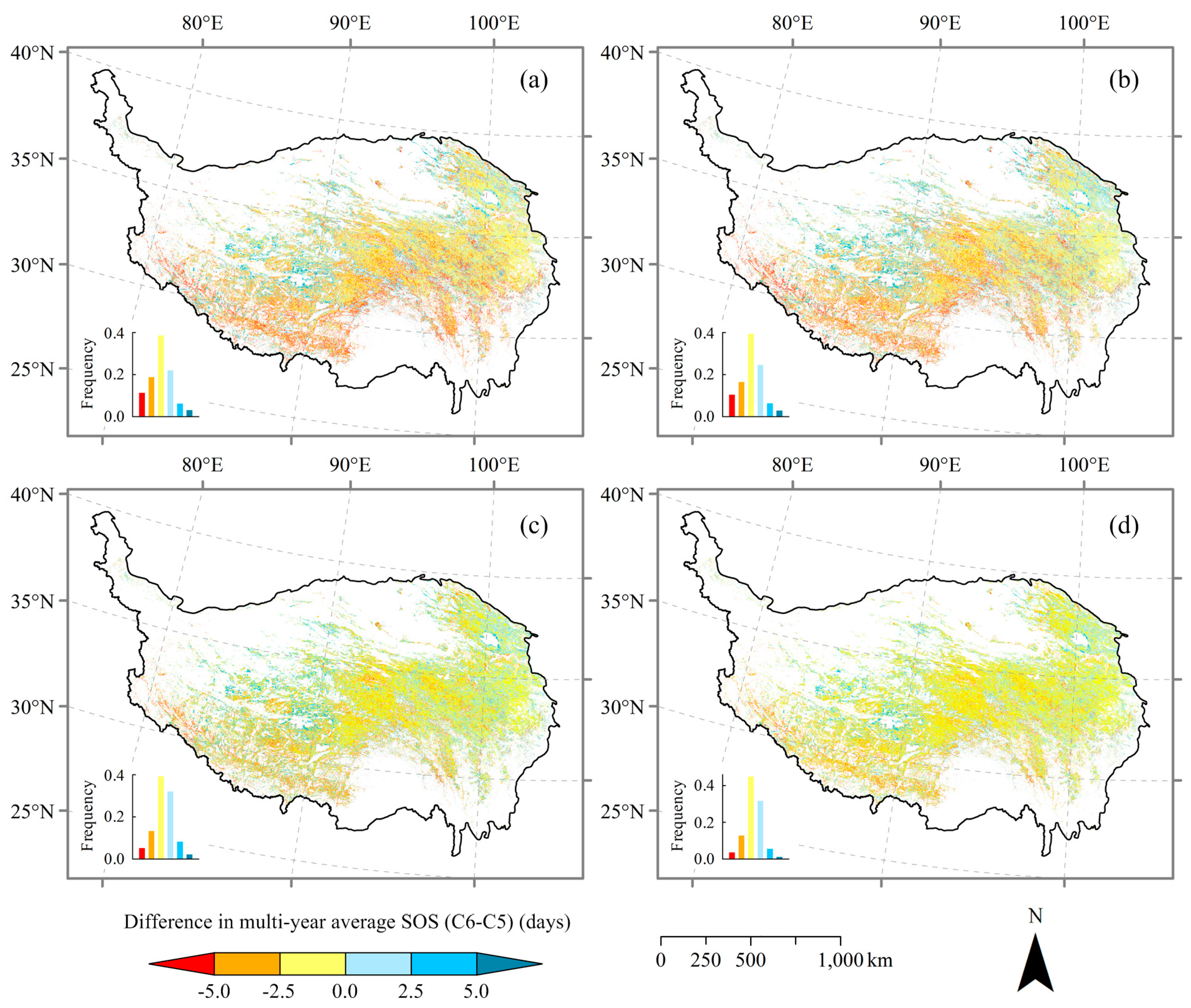
For each method, various degrees of differences between the multi-year average SOSC5 and SOSC6 were found (Figure 6). The multi-year average SOSC6 was earlier than the multi-year average SOSC5 for most of pixels (68.7% for MCC, 66.2% for DT2, 57.6% for DT5 and 61.6% for MS) (Figure 6). As for the pixels with differences of more than five days, SOS based on MCC and MS methods showed the largest (14.4%) and smallest (4.9%) proportions of the total area, respectively (Figure 6). The corresponding proportions for DT2 and DT5 methods were 13.2% and 7.4%, respectively. All four methods indicated that the pixels with SOSC6 later than SOSC5 were mainly distributed in the northwestern TP, while the differences between SOSC5 and SOSC6 varied with methods in the southern TP, with larger differences for MCC and DT2 methods and less for DT5 and MS methods (Figure 6).
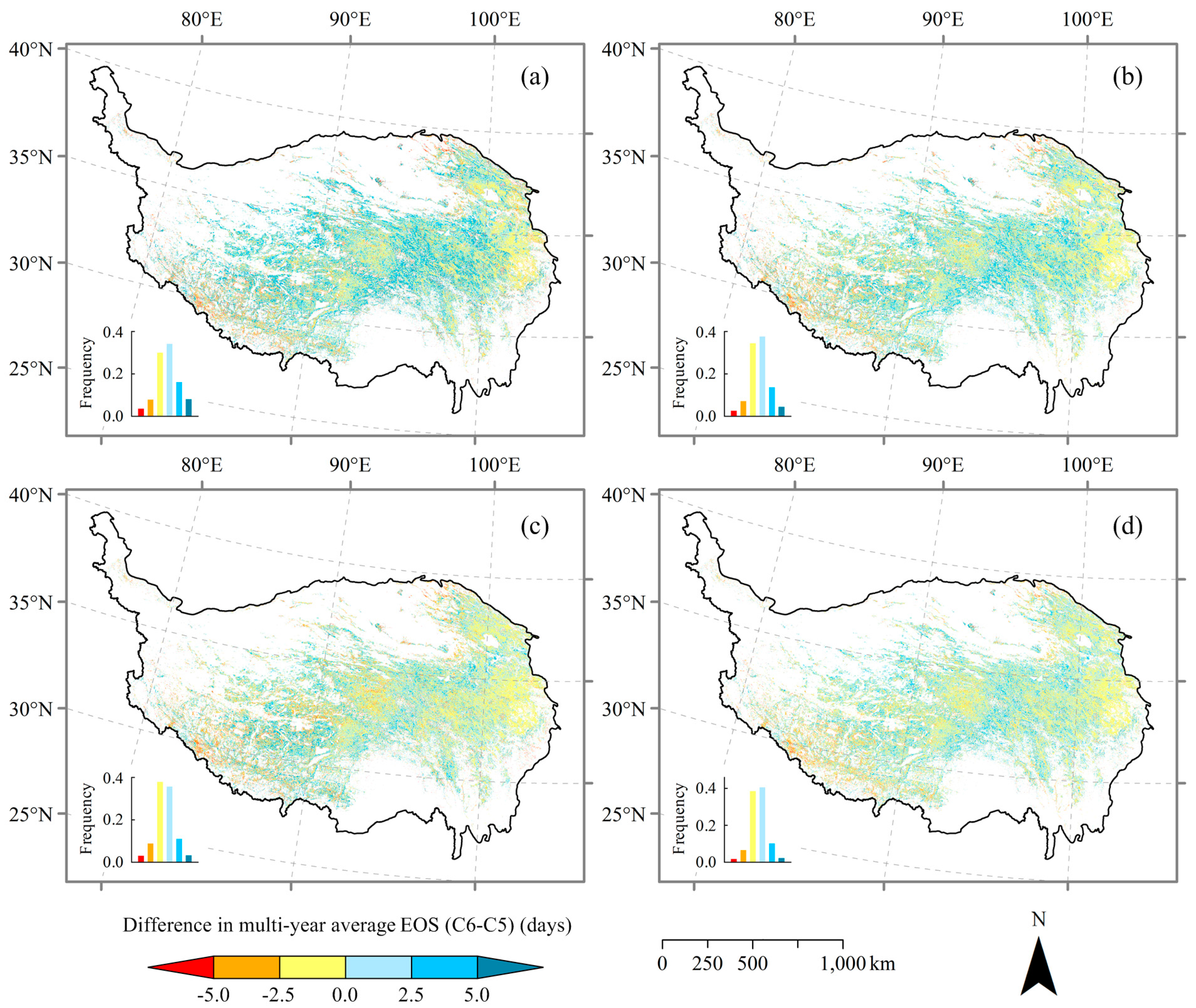
Similar to SOS, large differences were found for multi-year average EOSC5 and EOSC6 based on four methods (Figure 7). The EOSC6 was later than the EOSC5 over 58.5% of pixels for MCC method, while the proportions were 55.8%, 50.0%, and 53.1% for DT2, DT5, and MS methods, respectively (Figure 7). The pixels with the differences of more than five days between EOSC5 and EOSC6 accounted for 11.7%, 7.1%, 6.4% and 4.1% of the total area for MCC, DT2, DT5 and MS methods, respectively. For each method, the pixels where EOSC6 was earlier than EOSC5 were mainly distributed in the eastern and southwestern TP. The differences of EOS in the central TP were larger for MCC method than the other methods.
3.4. Spatial Differences in Phenological Trends
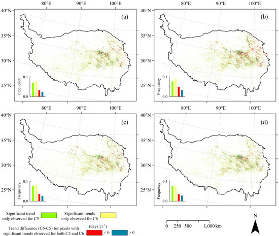
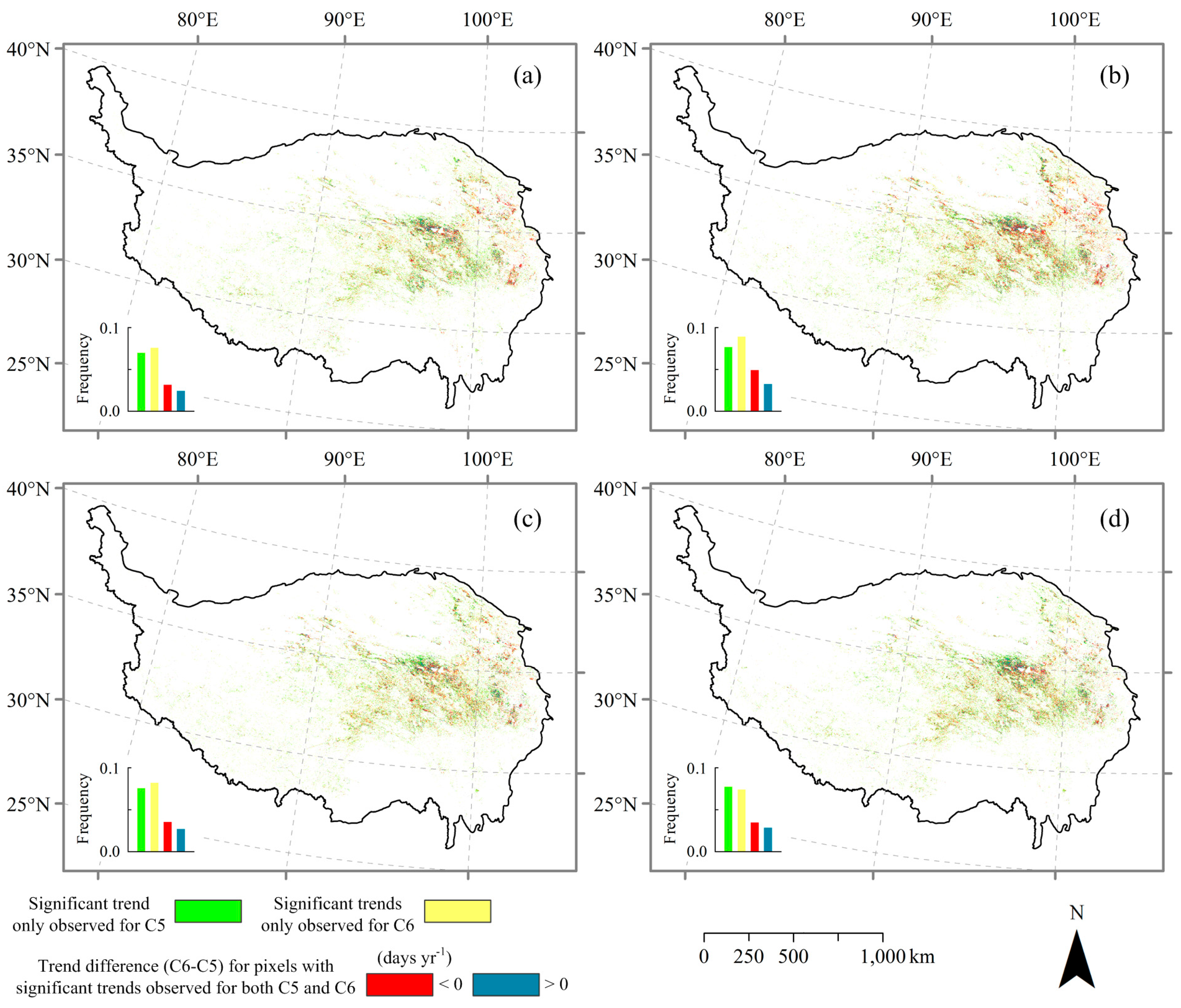
For each method, the proportion of advancing trends was much higher than that of delaying trends for both SOSC5 and SOSC6 (Table 2). The proportions of advancing (delaying) trends, as well as significantly advancing (delaying) trends (p < 0.05) in SOSC5 and SOSC6 were similar based on the same method (Table 2). However, the trends in SOSC5 and SOSC6 showed obvious spatial inconsistencies (Figure 8). For all four methods, the significant levels of SOS trends shifted over a considerable proportion of the study region. Significant trends in SOSC5 became insignificant in SOSC6 over 6.98%, 7.67%, 7.55%, and 7.74% of pixels for MCC, DT2, DT5, and MS methods, respectively (Figure 8). Meanwhile, insignificant trends in SOSC5 became significant in SOSC6 over 7.60%, 8.92%, 8.20%, and 7.42% of pixels for MCC, DT2, DT5, and MS methods, respectively (Figure 8). For the pixels with significant trends in both SOSC5 and SOSC6, SOS trends tended to be more negative from C5 to C6 for each method (Figure 8). Significant (p < 0.001) difference was observed between the SOS trends of C5 and C6 for each method, with mean differences between C5 and C6 (C6–C5) of −0.05, −0.07, −0.05, and −0.03 day yr−1 for MCC, DT2, DT5, and MS methods, respectively.
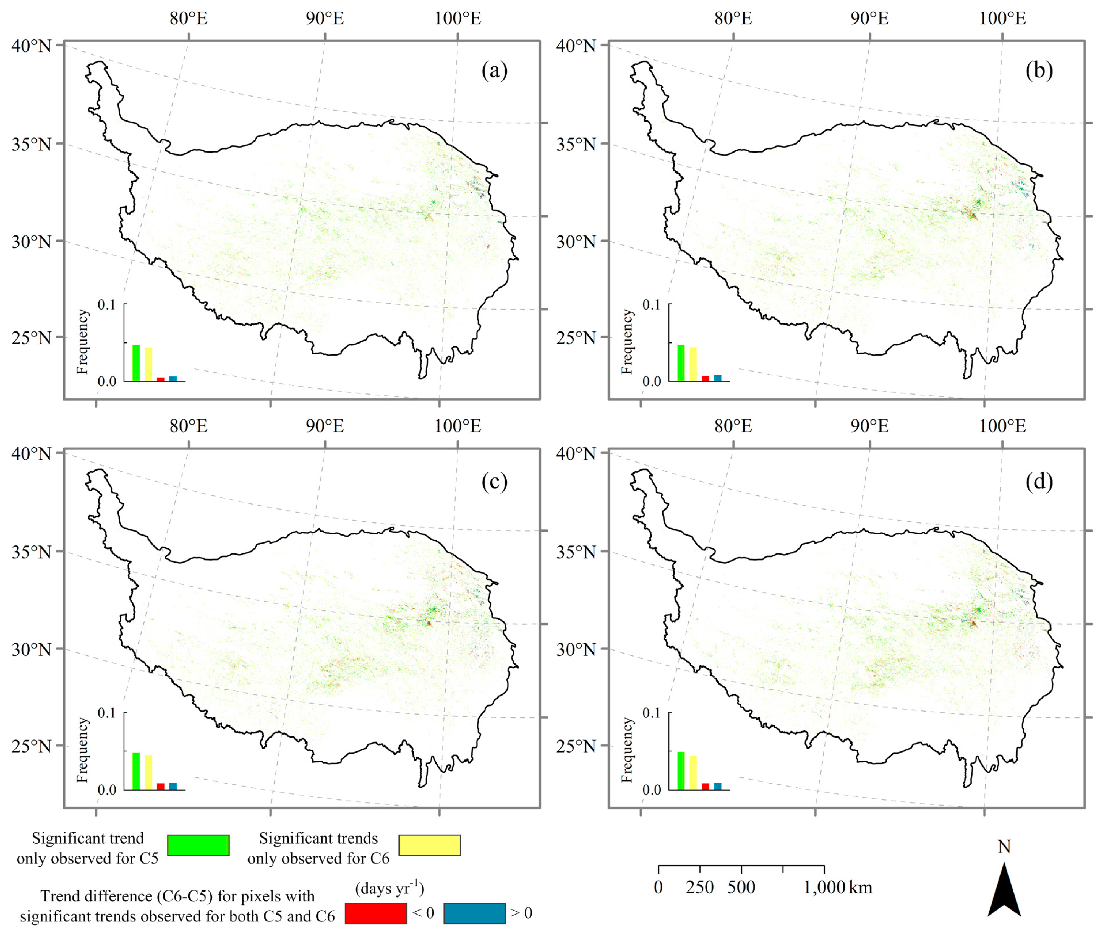
The proportion of advancing trends was higher than that of delaying trends for both EOSC5 and EOSC6 for each method (Table 3). Only a small proportion of significantly advancing or delaying trends was found for both EOSC5 and EOSC6 (Table 3). For each method, the advancing trends in EOSC6 accounted for a higher proportion of the total pixels than those in EOSC5, while the delaying trends in EOSC6 accounted for a lower proportion than those in EOSC5 (Table 3). Large spatial differences in trends between EOSC5 and EOSC6 were also found (Figure 9). From C5 to C6, pixels with a EOS trend shifting from significant to insignificant accounted for 4.70%, 4.71%, 4.80%, and 4.90% of the total pixels for MCC, DT2, DT5, and MS methods, respectively. Meanwhile, insignificant trends in EOSC5 became significant in EOSC6 over 4.37%, 4.41%, 4.51%, and 4.39% of pixels for MCC, DT2, DT5, and MS methods, respectively. Although a significant difference was also found between EOSC5 and EOSC6 trends (p < 0.001) for each method, a very small proportion of pixels with significant trends for both EOSC5 and EOSC6 was found for each method (1.18% for MCC, 1.54% for DT2, 1.75% for DT5, and 1.77% for MS) (Figure 9).
3.5. Comparison Between Satellite-Derived and Ground-Observed Phenology
The differences between the satellite-derived SOS (SOSC5 and SOSC6) and the ground-observed GU were smaller for MCC and DT2 methods and larger for DT5 and MS methods (Table 4). For both SOSC5 and SOSC6, the MEs and MAEs were about 10 days based on MCC and DT2 methods, but more than 30 days based on DT5 and MS methods (Table 4). However, SOSC5 had a slightly smaller ME or MAE than SOSC6 for each method (Table 4). Besides, both SOSC5 and SOSC6 were significantly and positively correlated with GU for all of the methods (p < 0.01), but the correlation coefficient between SOSC5 and GU was larger than that between SOSC6 and GU for each method (Table 4). Results based on MCC method showed the highest correlation coefficients between SOS and GU (Table 4).
However, large differences between the satellite-derived EOS (EOSC5 and EOSC6) and the ground-observed BLC were found. The MEs and MAEs of EOS were more than 18 days for each method (Table 4). Moreover, both EOSC5 and EOSC6 showed very poor positive correlations with BLC for all of the methods (Table 4). Nevertheless, the correlation between EOSC5 and BLC was still slightly higher than that between EOSC6 and BLC for each method (Table 4).
4. Discussion
The annual regional average GSNDVI for the alpine grassland on the TP showed no obvious trend for C5 (p = 0.424), but a significant increasing trend for C6 (p < 0.05) (Figure 1). Moreover, GSNDVIC6 showed increasing trends over more areas than GSNDVIC5 (Figure 3). These greening trends may result from the removal of sensor degradation, which can lead to a decline in NDVI, as previous studies suggested [12,13]. Zhang et al. [17] also reported that the annual NDVI from Terra C6 showed larger greening vegetation area than Terra C5 at global scale, which was consistent with the result of our study. Besides, in a comparative study of cross-product NDVI dynamics in a tropical region in Tanzania, significant increasing trends in NDVI also became more apparent in Terra C6 NDVI than C5 NDVI [20]. In this study, the regional average GSNDVIC6 was significantly lower than GSNDVIC5 (Figure 1). At spatial scale, the multi-year average GSNDVIC6 was lower than the GSNDVIC5 in most areas (Figure 2). These could cause the change of the NDVI curve shape, resulting in some differences between phenology derived from C5 and C6 NDVI [32].
The identified vegetation phenology can be affected by the phenology extraction methods [28]. To avoid the bias of a single phenology extraction method [21], this study applied four common methods to identify the vegetation phenological metrics. The identified SOSs from the earliest to the latest ranked by MCC, DT2, MS, and DT5 (Table 2), which was almost consistent with the study of Shen et al. [25]. Meanwhile, the order of the identified EOSs from the earliest to the latest was DT5, MS, DT2, and MCC (Table 3). The difference in average SOS and EOS could be more than one month among different methods. White et al. [28] found that individual methods differed in average SOS by ±60 days, and the spatial phenological patterns derived from different methods often differed among ecoregions by comparing 10 commonly used methods for estimating the SOS based on the Advanced Very High Resolution Radiometer (AVHRR) NDVI in North America. Such differences in phenology among methods were also found in other previous studies [33,34,35]. In our study, the differences between phenology derived from C5 and C6 NDVI varied among methods (Table 2 and Table 3, Figure 6, Figure 7, Figure 8 and Figure 9). Generally, most pixels showed an earlier multi-year average SOSC6 than SOSC5 and later EOSC6 than EOSC5 (Figure 6 and Figure 7). From C5 to C6, pixels with a SOS (EOS) trend changed from significant to insignificant, or from insignificant to significant accounted for at least 14.58% (9.07%) of the total pixels (Figure 8 and Figure 9). This further confirmed the influence of the change in NDVI values originated from sensor degradation and calibration methods on vegetation phenology monitoring.
By comparing the satellite-derived with the ground-observed phenology, SOS identified by MCC and DT2 methods was more consistent and correlated with the ground-observed GU than that by MS and DT5 methods for both C5 and C6 NDVI (Table 4), implying that MCC and DT2 methods were more suitable to monitor GU for the alpine grassland on the TP. Yu et al. [36] also found that SOS that was extracted by DT2 from AVHRR NDVI was close to the ground observations on the TP. Moreover, smaller differences and higher correlations were found between SOSC5 and GU than between SOSC6 and GU (Table 4), implying that SOSC5 might be more consistent than SOSC6 with the ground-observed GU. C5 NDVI may be more appropriate for monitoring SOS than C6 NDVI in this area, but more ground-observed phenology records are needed to confirm it due to only four available sites in our study. However, regarding EOS, large differences and poor correlations between EOSC5, as well as EOSC6 and BLC, were found for all of the phenology extraction methods (Table 4). When compared with SOS, EOS is much difficult to be monitored [37,38,39]. Many factors can influence the evaluation of vegetation phenology shifts based on remote sensing data [38,40]. When comparing the satellite-derived with the ground-observed phenology, due to the difference in observation scale (pixel versus individual plant) and content (spectral response of plant versus specific phenological event of plant), the satellite-derived phenology (e.g., EOS) is considered to be related, but not identical, to the ground-observed phenology (e.g., BLC) [28,41,42]. Therefore, it brings much uncertainty to the validation of the satellite-derived phenology. Besides, plants often experience a longer and slower change in canopy greenness in autumn than in spring [38,39,43], which may result in a lower inter-annual variability of changes in EOS relative to SOS and consequently make it more difficult to detect EOS from remote sensing time-series data [38]. Therefore, there is a need to use near-surface remote sensing data with a higher resolution, including digital camera data [44,45,46] and corresponding validation methods, for further evaluating the uncertainty in monitoring vegetation phenology with MODIS C5 and C6 NDVI products.
This study aimed to compare the differences between MODIS C5 and C6 NDVI time series in monitoring vegetation phenology on the TP. Based on the same selected grassland pixels, the same data pre-processing methods and phenology extraction methods, the differences in phenology derived from the two products were found to be mainly due to the sensor degradation and different calibration methods. However, it should be noted that the selection criteria for grassland pixels and the data pre-processing methods might influence the values of the satellite-derived phenological metrics. Besides, the satellite-derived phenology is also influenced by the temporal [47,48], spatial [49], and spectral resolutions [21] of remote sensing data.
5. Conclusions
This study conducted a comparative analysis of MODIS C5 and C6 NDVI-derived phenology for the alpine grassland on the TP. Although the regional average SOSC5 and SOSC6 (EOSC5 and EOSC6) showed consistent inter-annual variations, large spatial differences in trends between SOSC5 and SOSC6 (EOSC5 and EOSC6) were found. From C5 to C6, pixels with a SOS (EOS) trend changed from significant to insignificant, or from insignificant to significant, accounted for at least 14.58% (9.07%) of the total pixels. By comparing the satellite-derived phenology with the ground-observed phenology, SOSC5 was found to be more consistent than SOSC6 with the ground-observed green-up dates. C5 NDVI may be more appropriate for monitoring SOS than C6 NDVI in this area, but more ground-observed phenology records are needed to confirm it due to the only four available sites. However, both EOSC5 and EOSC6 showed large differences and poor correlations with the ground-observed beginning of leaf coloring. The accuracy of vegetation phenology derived from remote sensing data was impacted by many factors. Therefore, there is a need to use near-surface remote sensing data with a higher resolution and corresponding validation methods for further evaluating the uncertainty of MODIS C5 and C6 NDVI products in monitoring vegetation phenology.
Acknowledgments
The authors thank the editor and reviewers for helpful comments and suggestions. The authors also thank the Meteorological Information Center of the China Meteorological Administration for providing phenology data. This work was supported by National Natural Science Foundation of China (Grant No. 41371389, No. 41771047) and the project from State Key Laboratory of Earth Surface Processes and Resource Ecology (Grant No. 2017-FX-01(1)).
Author Contributions
Zhoutao Zheng and Wenquan Zhu designed this study and wrote the manuscript; Zhoutao Zheng performed the data pre-processing; Zhoutao Zheng and Wenquan Zhu conducted the analysis.
Conflicts of Interest
The authors declare no conflict of interest.
References
- Cleland, E.E.; Chuine, I.; Menzel, A.; Mooney, H.A.; Schwartz, M.D. Shifting plant phenology in response to global change. Trends Ecol. Evol. 2007, 22, 357–365. [Google Scholar] [CrossRef] [PubMed]
- Richardson, A.D.; Keenan, T.F.; Migliavacca, M.; Ryu, Y.; Sonnentag, O.; Toomey, M. Climate change, phenology, and phenological control of vegetation feedbacks to the climate system. Agric. For. Meteorol. 2013, 169, 156–173. [Google Scholar] [CrossRef]
- Piao, S.L.; Friedlingstein, P.; Ciais, P.; Viovy, N.; Demarty, J. Growing season extension and its impact on terrestrial carbon cycle in the Northern Hemisphere over the past 2 decades. Glob. Biogeochem. Cycles 2007, 21, GB30183. [Google Scholar] [CrossRef]
- Jeong, S.J.; Ho, C.H.; Gim, H.J.; Brown, M.E. Phenology shifts at start vs. end of growing season in temperate vegetation over the Northern Hemisphere for the period 1982–2008. Glob. Chang. Biol. 2011, 17, 2385–2399. [Google Scholar] [CrossRef]
- Zhu, W.Q.; Tian, H.Q.; Xu, X.F.; Pan, Y.Z.; Chen, G.S.; Lin, W.P. Extension of the growing season due to delayed autumn over mid and high latitudes in North America during 1982–2006. Glob. Ecol. Biogeogr. 2012, 21, 260–271. [Google Scholar] [CrossRef]
- Piao, S.; Wang, X.; Ciais, P.; Zhu, B.; Wang, T.; Liu, J. Changes in satellite-derived vegetation growth trend in temperate and boreal Eurasia from 1982 to 2006. Glob. Chang. Biol. 2011, 17, 3228–3239. [Google Scholar] [CrossRef]
- Jönsson, P.; Eklundh, L. Seasonality extraction by function fitting to time-series of satellite sensor data. IEEE Trans. Geosci. Remote Sens. 2002, 40, 1824–1832. [Google Scholar] [CrossRef]
- Stockli, R.; Vidale, P.L. European plant phenology and climate as seen in a 20-year AVHRR land-surface parameter dataset. Int. J. Remote Sens. 2004, 25, 3303–3330. [Google Scholar] [CrossRef]
- Zhang, G.L.; Zhang, Y.J.; Dong, J.W.; Xiao, X.M. Green-up dates in the Tibetan Plateau have continuously advanced from 1982 to 2011. Proc. Natl. Acad. Sci. USA 2013, 110, 4309–4314. [Google Scholar] [CrossRef] [PubMed]
- Djavidnia, S.; Melin, F.; Hoepffner, N. Comparison of global ocean colour data records. Ocean Sci. 2010, 6, 61–76. [Google Scholar] [CrossRef]
- Levy, R.C.; Remer, L.A.; Kleidman, R.G.; Mattoo, S.; Ichoku, C.; Kahn, R.; Eck, T.F. Global evaluation of the Collection 5 MODIS dark-target aerosol products over land. Atmos. Chem. Phys. 2010, 10, 10399–10420. [Google Scholar] [CrossRef] [Green Version]
- Lyapustin, A.; Wang, Y.; Xiong, X.; Meister, G.; Platnick, S.; Levy, R.; Franz, B.; Korkin, S.; Hilker, T.; Tucker, J.; et al. Scientific impact of MODIS C5 calibration degradation and C6+ improvements. Atmos. Meas. Tech. 2014, 7, 4353–4365. [Google Scholar] [CrossRef]
- Wang, D.; Morton, D.; Masek, J.; Wu, A.; Nagol, J.; Xiong, X.; Levy, R.; Vermote, E.; Wolfe, R. Impact of sensor degradation on the MODIS NDVI time series. Remote Sens. Environ. 2012, 119, 55–61. [Google Scholar] [CrossRef]
- Zhao, M.; Running, S.W. Response to comments on “Drought-induced reduction in global terrestrial net primary production from 2000 through 2009”. Science 2011, 333, 1093. [Google Scholar] [CrossRef]
- Vermote, E.F.; El Saleous, N.Z.; Justice, C.O. Atmospheric correction of MODIS data in the visible to middle infrared: First results. Remote Sens. Environ. 2002, 83, 97–111. [Google Scholar] [CrossRef]
- Kotchenova, S.Y.; Vermote, E.F.; Levy, R.; Lyapustin, A. Radiative transfer codes for atmospheric correction and aerosol retrieval: Intercomparison study. Appl. Opt. 2008, 47, 2215–2226. [Google Scholar] [CrossRef] [PubMed]
- Zhang, Y.; Song, C.; Band, L.E.; Sun, G.; Li, J. Reanalysis of global terrestrial vegetation trends from MODIS products: Browning or greening? Remote Sens. Environ. 2017, 191, 145–155. [Google Scholar] [CrossRef]
- Toller, G.; Xiong, X.; Sun, J.; Wenny, B.N.; Geng, X.; Kuyper, J.; Angal, A.; Chen, H.; Madhavan, S.; Wua, A. Terra and Aqua moderate-resolution imaging spectroradiometer collection 6 level 1B algorithm. J. Appl. Remote Sens. 2013, 7, 073557. [Google Scholar] [CrossRef]
- Didan, K.; Munoz, A.B.; Solano, R.; Huete, A. MODIS Vegetation Index Users Guide (MOD13 Series); Version 3.00 (Collection 6); Vegetation Index and Phenology Lab, The University of Arizona: Tucson, AZ, USA, 2015. [Google Scholar]
- Detsch, F.; Otte, I.; Appelhans, T.; Nauss, T. A comparative study of cross-product NDVI dynamics in the Kilimanjaro region a matter of sensor, degradation calibration, and significance. Remote Sens. 2016, 8, 159. [Google Scholar] [CrossRef]
- Atzberger, C.; Klisch, A.; Mattiuzzi, M.; Vuolo, F. Phenological metrics derived over the European continent from NDVI3g data and MODIS time series. Remote Sens. 2014, 6, 257–284. [Google Scholar] [CrossRef]
- Xin, Q.; Broich, M.; Zhu, P.; Gong, P. Modeling grassland spring onset across the Western United States using climate variables and MODIS-derived phenology metrics. Remote Sens. Environ. 2015, 161, 63–77. [Google Scholar] [CrossRef]
- Zeng, H.; Jia, G.; Epstein, H. Recent changes in phenology over the northern high latitudes detected from multi-satellite data. Environ. Res. Lett. 2011, 6, 045508. [Google Scholar] [CrossRef]
- Chen, X. East Asia. In Phenology: An Integrative Environmental Science, 2nd ed.; Schwartz, M.D., Ed.; Springer: Dordrecht, The Netherlands, 2013; pp. 9–22. [Google Scholar]
- Shen, M.G.; Zhang, G.X.; Cong, N.; Wang, S.P.; Kong, W.D.; Piao, S.L. Increasing altitudinal gradient of spring vegetation phenology during the last decade on the Qinghai-Tibetan Plateau. Agric. For. Meteorol. 2014, 189–190, 71–80. [Google Scholar] [CrossRef]
- Chen, J.; Jonsson, P.; Tamura, M.; Gu, Z.H.; Matsushita, B.; Eklundh, L. A simple method for reconstructing a high-quality NDVI time-series data set based on the Savitzky-Golay filter. Remote Sens. Environ. 2004, 91, 332–344. [Google Scholar] [CrossRef]
- Ding, M.; Zhang, Y.; Sun, X.; Liu, L.; Wang, Z.; Bai, W. Spatiotemporal variation in alpine grassland phenology in the Qinghai-Tibetan Plateau from 1999 to 2009. Chin. Sci. Bull. 2013, 58, 396–405. [Google Scholar] [CrossRef]
- White, M.A.; Beurs, D.; Kirsten, M.; Didan, K.; Inouye, D.W.; Richardson, A.D.; Jensen, O.P.; O’Keefe, J.; Zhang, G.; Nemani, R.R.; et al. Intercomparison, interpretation, and assessment of spring phenology in North America estimated from remote sensing for 1982–2006. Glob. Chang. Biol. 2009, 15, 2335–2359. [Google Scholar] [CrossRef]
- Zhang, X.Y.; Friedl, M.A.; Schaaf, C.B.; Strahler, A.H.; Hodges, J.; Gao, F.; Reed, B.C.; Huete, A. Monitoring vegetation phenology using MODIS. Remote Sens. Environ. 2003, 84, 471–475. [Google Scholar] [CrossRef]
- White, M.A.; Thornton, P.E.; Running, S.W. A continental phenology model for monitoring vegetation responses to interannual climatic variability. Glob. Biogeochem. Cycles 1997, 11, 217–234. [Google Scholar] [CrossRef]
- Studer, S.; Stoeckli, R.; Appenzeller, C.; Vidale, P.L. A comparative study of satellite and ground-based phenology. Int. J. Biometeorol. 2007, 51, 405–414. [Google Scholar] [CrossRef] [PubMed]
- Luo, X.; Chen, X.; Xu, L.; Myneni, R.; Zhu, Z. Assessing performance of NDVI and NDVI3g in monitoring leaf unfolding dates of the deciduous broadleaf forest in northern china. Remote Sens. 2013, 5, 845–861. [Google Scholar] [CrossRef]
- Ding, M.; Li, L.; Zhang, Y.; Sun, X.; Liu, L.; Gao, J.; Wang, Z.; Li, Y. Start of vegetation growing season on the Tibetan Plateau inferred from multiple methods based on GIMMS and SPOT NDVI data. J. Geogr. Sci. 2015, 25, 131–148. [Google Scholar] [CrossRef]
- Cong, N.; Piao, S.L.; Chen, A.P.; Wang, X.H.; Lin, X.; Chen, S.P.; Han, S.J.; Zhou, G.S.; Zhang, X.P. Spring vegetation green-up date in China inferred from SPOT NDVI data: A multiple model analysis. Agric. For. Meteorol. 2012, 165, 104–113. [Google Scholar] [CrossRef]
- Chang, Q.; Zhang, J.; Jiao, W.; Yao, F. A comparative analysis of the NDVIg and NDVI3g in monitoring vegetation phenology changes in the Northern Hemisphere. Geocarto Int. 2016, 33, 1–20. [Google Scholar] [CrossRef]
- Yu, H.Y.; Luedeling, E.; Xu, J.C. Winter and spring warming result in delayed spring phenology on the Tibetan Plateau. Proc. Natl. Acad. Sci. USA 2010, 107, 22151–22156. [Google Scholar] [CrossRef] [PubMed]
- Jeong, S.; Schimel, D.; Frankenberg, C.; Drewry, D.T.; Fisher, J.B.; Verma, M.; Berry, J.A.; Lee, J.; Joiner, J. Application of satellite solar-induced chlorophyll fluorescence to understanding large-scale variations in vegetation phenology and function over northern high latitude forests. Remote Sens. Environ. 2017, 190, 178–187. [Google Scholar] [CrossRef]
- Wu, C.; Peng, D.; Soudani, K.; Siebicke, L.; Gough, C.M.; Arain, M.A.; Bohrer, G.; Lafleur, P.M.; Peichl, M.; Gonsamo, A.; et al. Land surface phenology derived from normalized difference vegetation index (NDVI) at global FLUXNET sites. Agric. For. Meteorol. 2017, 233, 171–182. [Google Scholar] [CrossRef]
- Liu, Y.; Wu, C.; Peng, D.; Xu, S.; Gonsamo, A.; Jassal, R.S.; Arain, M.A.; Lu, L.; Fang, B.; Chen, J.M. Improved modeling of land surface phenology using MODIS land surface reflectance and temperature at evergreen needleleaf forests of central North America. Remote Sens. Environ. 2016, 176, 152–162. [Google Scholar] [CrossRef]
- Peng, D.; Zhang, X.; Wu, C.; Huang, W.; Gonsamo, A.; Huete, A.R.; Didan, K.; Tan, B.; Liu, X.; Zhang, B. Intercomparison and evaluation of spring phenology products using National Phenology Network and AmeriFlux observations in the contiguous United States. Agric. For. Meteorol. 2017, 242, 33–46. [Google Scholar] [CrossRef]
- Badeck, F.W.; Bondeau, A.; Bottcher, K.; Doktor, D.; Lucht, W.; Schaber, J.; Sitch, S. Responses of spring phenology to climate change. New Phytol. 2004, 162, 295–309. [Google Scholar] [CrossRef]
- Xu, H.; Twine, T.E.; Yang, X. Evaluating remotely sensed phenological metrics in a dynamic ecosystem model. Remote Sens. 2014, 6, 4660–4686. [Google Scholar] [CrossRef]
- Gallinat, A.S.; Primack, R.B.; Wagner, D.L. Autumn, the neglected season in climate change research. Trends Ecol. Evol. 2015, 30, 169–176. [Google Scholar] [CrossRef] [PubMed]
- Migliavacca, M.; Galvagno, M.; Cremonese, E.; Rossini, M.; Meroni, M.; Sonnentag, O.; Cogliati, S.; Manca, G.; Diotri, F.; Busetto, L.; et al. Using digital repeat photography and eddy covariance data to model grassland phenology and photosynthetic CO2 uptake. Agric. For. Meteorol. 2011, 151, 1325–1337. [Google Scholar] [CrossRef]
- Richardson, A.D.; Hollinger, D.Y.; Dail, D.B.; Lee, J.T.; Munger, J.W.; O’Keefe, J. Influence of spring phenology on seasonal and annual carbon balance in two contrasting New England forests. Tree Physiol. 2009, 29, 321–331. [Google Scholar] [CrossRef] [PubMed]
- Sonnentag, O.; Hufkens, K.; Teshera-Sterne, C.; Young, A.M.; Friedl, M.; Braswell, B.H.; Milliman, T.; O'Keefe, J.; Richardson, A.D. Digital repeat photography for phenological research in forest ecosystems. Agric. For. Meteorol. 2012, 152, 159–177. [Google Scholar] [CrossRef]
- Zhang, X.; Friedl, M.A.; Schaaf, C.B. Sensitivity of vegetation phenology detection to the temporal resolution of satellite data. Int. J. Remote Sens. 2009, 30, 2061–2074. [Google Scholar] [CrossRef]
- Kross, A.; Fernandes, R.; Seaquist, J.; Beaubien, E. The effect of the temporal resolution of NDVI data on season onset dates and trends across Canadian broadleaf forests. Remote Sens. Environ. 2011, 115, 1564–1575. [Google Scholar] [CrossRef]
- Klosterman, S.T.; Hufkens, K.; Gray, J.M.; Melaas, E.; Sonnentag, O.; Lavine, I.; Mitchell, L.; Norman, R.; Friedl, M.A.; Richardson, A.D. Evaluating remote sensing of deciduous forest phenology at multiple spatial scales using PhenoCam imagery. Biogeosciences 2014, 11, 4305–4320. [Google Scholar] [CrossRef] [Green Version]
Figure 1.
Comparison of annual regional average growing season Normalized Difference Vegetation Index derived from MODIS C5 (GSNDVIC5) and C6 (GSNDVIC6) for the alpine grassland on the Tibetan Plateau during 2001–2015.
Figure 1.
Comparison of annual regional average growing season Normalized Difference Vegetation Index derived from MODIS C5 (GSNDVIC5) and C6 (GSNDVIC6) for the alpine grassland on the Tibetan Plateau during 2001–2015.

Figure 2.
(a) The relative difference in the multi-year average growing season Normalized Difference Vegetation Index between C6 (GSNDVIC6) and C5 (GSNDVIC5) ((C6–C5)/C5) during 2001–2015; (b) The scatter plot of the multi-year average GSNDVIC6 against GSNDVIC5 during 2001–2015.
Figure 2.
(a) The relative difference in the multi-year average growing season Normalized Difference Vegetation Index between C6 (GSNDVIC6) and C5 (GSNDVIC5) ((C6–C5)/C5) during 2001–2015; (b) The scatter plot of the multi-year average GSNDVIC6 against GSNDVIC5 during 2001–2015.

Figure 3.
(a) Comparison of trends in growing season Normalized Difference Vegetation Index between C5 (GSNDVIC5) and C6 (GSNDVIC6) during 2001–2015; and, (b) The histograms of trends in GSNDVIC5 and GSNDVIC6 during 2001–2015.
Figure 3.
(a) Comparison of trends in growing season Normalized Difference Vegetation Index between C5 (GSNDVIC5) and C6 (GSNDVIC6) during 2001–2015; and, (b) The histograms of trends in GSNDVIC5 and GSNDVIC6 during 2001–2015.

Figure 4.
Comparisons of annual regional average start of growing season from MODIS C5 (SOSC5) and C6 (SOSC6) for the alpine grassland on the Tibetan Plateau during 2001–2015 for different methods: (a) Maximum Curvature Change (MCC); (b) Dynamic Threshold 0.2 (DT2); (c) Dynamic Threshold 0.5 (DT5); and, (d) Maximum Slope (MS).

Figure 5.
Comparisons of annual regional average end of growing season from MODIS C5 (SOSC5) and C6 (SOSC6) for the alpine grassland on the Tibetan Plateau during 2001–2015 for different methods: (a) Maximum Curvature Change (MCC); (b) Dynamic Threshold 0.2 (DT2); (c) Dynamic Threshold 0.5 (DT5); (d) Maximum Slope (MS).

Figure 6.
Spatial differences between the multi-year average SOSC6 and SOSC5 (C6–C5) for different methods: (a) Maximum Curvature Change (MCC); (b) Dynamic Threshold 0.2 (DT2); (c) Dynamic Threshold 0.5 (DT5); (d) Maximum Slope (MS).
Figure 6.
Spatial differences between the multi-year average SOSC6 and SOSC5 (C6–C5) for different methods: (a) Maximum Curvature Change (MCC); (b) Dynamic Threshold 0.2 (DT2); (c) Dynamic Threshold 0.5 (DT5); (d) Maximum Slope (MS).

Figure 7.
Spatial differences between the multi-year average EOSC6 and EOSC5 (C6–C5) for different methods: (a) Maximum Curvature Change (MCC); (b) Dynamic Threshold 0.2 (DT2); (c) Dynamic Threshold 0.5 (DT5); and, (d) Maximum Slope (MS).
Figure 7.
Spatial differences between the multi-year average EOSC6 and EOSC5 (C6–C5) for different methods: (a) Maximum Curvature Change (MCC); (b) Dynamic Threshold 0.2 (DT2); (c) Dynamic Threshold 0.5 (DT5); and, (d) Maximum Slope (MS).

Figure 8.
Comparison of trends in start of growing season between C5 (SOSC5) and C6 (SOSC6) during 2001–2015 for different methods: (a) Maximum Curvature Change (MCC); (b) Dynamic Threshold 0.2 (DT2); (c) Dynamic Threshold 0.5 (DT5); and, (d) Maximum Slope (MS).
Figure 8.
Comparison of trends in start of growing season between C5 (SOSC5) and C6 (SOSC6) during 2001–2015 for different methods: (a) Maximum Curvature Change (MCC); (b) Dynamic Threshold 0.2 (DT2); (c) Dynamic Threshold 0.5 (DT5); and, (d) Maximum Slope (MS).

Figure 9.
Comparison of trends in end of growing season between C5 (EOSC5) and C6 (EOSC6) during 2001–2015 for different methods: (a) Maximum Curvature Change (MCC); (b) Dynamic Threshold 0.2 (DT2); (c) Dynamic Threshold 0.5 (DT5); and, (d) Maximum Slope (MS).
Figure 9.
Comparison of trends in end of growing season between C5 (EOSC5) and C6 (EOSC6) during 2001–2015 for different methods: (a) Maximum Curvature Change (MCC); (b) Dynamic Threshold 0.2 (DT2); (c) Dynamic Threshold 0.5 (DT5); and, (d) Maximum Slope (MS).


Table 1.
Summary of ground-observed phenology data of Kobresia humilis.
| Site Name | Longitude | Latitude | Altitude (m) | Number of Years |
|---|---|---|---|---|
| Haiyan | 100°51’E | 36°37’N | 3140 | 12 |
| Gande | 99°54’E | 33°58’N | 4050 | 12 |
| Henan | 101°36’E | 34°44’N | 3500 | 12 |
| Qumarleb | 95°47’E | 34°08’N | 4175 | 12 |
Table 2.
Summary statistics for the regional average start of growing season derived from C5 and C6 NDVI products for the alpine grassland on the Tibetan Plateau during 2001–2015.
Table 2.
Summary statistics for the regional average start of growing season derived from C5 and C6 NDVI products for the alpine grassland on the Tibetan Plateau during 2001–2015.
| Method | MCC | DT2 | DT5 | MS | ||||
|---|---|---|---|---|---|---|---|---|
| Product | C5 | C6 | C5 | C6 | C5 | C6 | C5 | C6 |
| Mean | 130.5 | 129.2 | 139.6 | 138.4 | 169.8 | 169.3 | 163.6 | 163.0 |
| Std | 2.5 | 2.6 | 2.9 | 3.0 | 2.7 | 2.8 | 2.5 | 2.6 |
| Trend | −0.278 | −0.298 | −0.339 | −0.378 | −0.312 | −0.332 | −0.258 | −0.264 |
| p value | 0.060 | 0.050 | 0.043 | 0.028 | 0.047 | 0.040 | 0.088 | 0.091 |
| Dall | 30.79% | 30.59% | 26.87% | 26.37% | 27.91% | 27.70% | 28.65% | 29.31% |
| Dsig | 1.18% | 1.17% | 0.91% | 0.79% | 1.00% | 0.93% | 1.01% | 1.03% |
| Aall | 69.2% | 69.4% | 73.13% | 73.63% | 72.09% | 72.30% | 71.35% | 70.69% |
| Asig | 11.39% | 12.03% | 14.95% | 16.31% | 12.80% | 13.52% | 13.08% | 12.75% |
Mean: multi-year average regional SOS. Std: temporal standard deviation. Trend: slope of linear regression of regional average SOS against year (days yr−1). p value: significance level for the trend. Aall and Dall: proportions of advancing and delaying trends, respectively. Asig and Dsig: proportions of significantly (p < 0.05) advancing and delaying trends, respectively.
Table 3.
Summary statistics for the regional average end of growing season derived from C5 and C6 Normalized Difference Vegetation Index (NDVI) products for the alpine grassland on the Tibetan Plateau during 2001–2015.
Table 3.
Summary statistics for the regional average end of growing season derived from C5 and C6 Normalized Difference Vegetation Index (NDVI) products for the alpine grassland on the Tibetan Plateau during 2001–2015.
| Method | MCC | DT2 | DT5 | MS | ||||
|---|---|---|---|---|---|---|---|---|
| Product | C5 | C6 | C5 | C6 | C5 | C6 | C5 | C6 |
| Mean | 312.3 | 313.0 | 303.0 | 303.5 | 272.5 | 272.6 | 279.1 | 279.3 |
| Std | 2.2 | 1.9 | 2.5 | 2.2 | 2.3 | 2.1 | 2.3 | 2.1 |
| Trend | −0.060 | 0.010 | −0.068 | −0.018 | −0.101 | −0.067 | −0.093 | −0.061 |
| p value | 0.665 | 0.929 | 0.670 | 0.895 | 0.490 | 0.622 | 0.523 | 0.645 |
| Dall | 43.75% | 49.75% | 42.53% | 47.09% | 39.66% | 42.38% | 39.64% | 42.83% |
| Dsig | 1.96% | 2.80% | 1.90% | 2.54% | 1.66% | 2.00% | 1.49% | 1.85% |
| Aall | 56.25% | 50.25% | 57.47% | 52.91% | 60.34% | 57.62% | 60.36% | 57.17% |
| Asig | 3.91% | 2.75% | 4.35% | 3.40% | 4.89% | 4.26% | 5.18% | 4.31% |
Mean: multi-year average regional EOS. Std: temporal standard deviation. Trend: slope of linear regression of regional average EOS against year (days yr−1). p value: significance level for the trend. Aall and Dall: proportions of advancing and delaying trends, respectively. Asig and Dsig: proportions of significantly (p < 0.05) advancing and delaying trends, respectively.
Table 4.
Mean error (ME), mean absolute error (MAE) and correlation coefficient (r) between the satellite-derived phenology and the ground-observed phenology.
Table 4.
Mean error (ME), mean absolute error (MAE) and correlation coefficient (r) between the satellite-derived phenology and the ground-observed phenology.
| Method | Phenological Metric | ME | MAE | r |
|---|---|---|---|---|
| MCC | SOSC5 | −7.375 | 9.542 | 0.675 ** |
| SOSC6 | −7.979 | 10.479 | 0.637 ** | |
| EOSC5 | 60.354 | 60.354 | 0.073 | |
| EOSC6 | 59.896 | 59.896 | 0.067 | |
| DT2 | SOSC5 | 4.146 | 9.479 | 0.580 ** |
| SOSC6 | 4.271 | 9.688 | 0.538 ** | |
| EOSC5 | 48.979 | 48.979 | 0.172 | |
| EOSC6 | 48.396 | 48.396 | 0.164 | |
| DT5 | SOSC5 | 35.125 | 35.125 | 0.532 ** |
| SOSC6 | 35.417 | 35.417 | 0.478 ** | |
| EOSC5 | 18.813 | 19.521 | 0.207 | |
| EOSC6 | 18.292 | 18.750 | 0.180 | |
| MS | SOSC5 | 30.771 | 30.771 | 0.526 ** |
| SOSC6 | 30.833 | 30.833 | 0.464 ** | |
| EOSC5 | 22.563 | 22.729 | 0.178 | |
| EOSC6 | 22.375 | 22.375 | 0.175 |
** indicates p < 0.01.
© 2017 by the authors. Licensee MDPI, Basel, Switzerland. This article is an open access article distributed under the terms and conditions of the Creative Commons Attribution (CC BY) license (http://creativecommons.org/licenses/by/4.0/).
Share and Cite
MDPI and ACS Style
Zheng, Z.; Zhu, W. Uncertainty of Remote Sensing Data in Monitoring Vegetation Phenology: A Comparison of MODIS C5 and C6 Vegetation Index Products on the Tibetan Plateau. Remote Sens. 2017, 9, 1288. https://doi.org/10.3390/rs9121288
AMA Style
Zheng Z, Zhu W. Uncertainty of Remote Sensing Data in Monitoring Vegetation Phenology: A Comparison of MODIS C5 and C6 Vegetation Index Products on the Tibetan Plateau. Remote Sensing. 2017; 9(12):1288. https://doi.org/10.3390/rs9121288
Chicago/Turabian StyleZheng, Zhoutao, and Wenquan Zhu. 2017. "Uncertainty of Remote Sensing Data in Monitoring Vegetation Phenology: A Comparison of MODIS C5 and C6 Vegetation Index Products on the Tibetan Plateau" Remote Sensing 9, no. 12: 1288. https://doi.org/10.3390/rs9121288
Note that from the first issue of 2016, this journal uses article numbers instead of page numbers. See further details here.