Google Earth Engine, Open-Access Satellite Data, and Machine Learning in Support of Large-Area Probabilistic Wetland Mapping

Abstract

Modern advances in cloud computing and machine-leaning algorithms are shifting the manner in which Earth-observation (EO) data are used for environmental monitoring, particularly as we settle into the era of free, open-access satellite data streams. Wetland delineation represents a particularly worthy application of this emerging research trend, since wetlands are an ecologically important yet chronically under-represented component of contemporary mapping and monitoring programs, particularly at the regional and national levels. Exploiting Google Earth Engine and R Statistical software, we developed a workflow for predicting the probability of wetland occurrence using a boosted regression tree machine-learning framework applied to digital topographic and EO data. Working in a 13,700 km² study area in northern Alberta, our best models produced excellent results, with AUC (area under the receiver-operator characteristic curve) values of 0.898 and explained-deviance values of 0.708. Our results demonstrate the central role of high-quality topographic variables for modeling wetland distribution at regional scales. Including optical and/or radar variables into the workflow substantially improved model performance, though optical data performed slightly better. Converting our wetland probability-of-occurrence model into a binary Wet-Dry classification yielded an overall accuracy of 85%, which is virtually identical to that derived from the Alberta Merged Wetland Inventory (AMWI): the contemporary inventory used by the Government of Alberta. However, our workflow contains several key advantages over that used to produce the AMWI, and provides a scalable foundation for province-wide monitoring initiatives.

1. Introduction

1.1. Trends in Satellite-Data Availability, Cloud Computing, and Machine Learning

The manner in which geospatial data sets are used for the mapping, monitoring, and study of Earth’s systems and environments has recently begun to shift in response to three notable trends in the geospatial sciences: (i) the proliferation of open-access satellite data streams, (ii) the advent of cloud computing, and (iii) the growing use of machine-learning algorithms. Not only are far greater volumes of Earth Observation (EO) satellite data available, but the processing and integration of diverse, large-volume data sets is possible with far greater ease, and by a larger number of users than ever before. This combination of factors has opened the doors to broader sets of applications at new spatial and temporal scales that were, until recently, simply impractical or infeasible in the majority of cases.

While Landsat offers the longest open-access EO data archive [1], other satellite sensors offering open-access data sets that complement Landsat are also available (e.g., Advanced Very High Resolution Radiometer (AVHRR), Advanced Spaceborne Thermal Emission and Reflection Radiameter (ASTER), Shuttle Radar Topography Mission (SRTM)), and have themselves been the focus of numerous large-scale mapping efforts. More recently, the European Space Agency’s Sentinel satellite series have begun offering high-resolution EO data at frequent intervals, representing important extensions to existing data streams [2].

Complementing the large volumes of open-access satellite data streams are the concurrent advent and growing availability of cloud-computing technologies and services. Downloading, analyzing and managing a multi-decadal time series of satellite images over large areas is not feasible using desktop computing resources. However, with the advent of services such as Google Earth Engine [3], the NASA Earth Exchange [4], Amazon’s Web Services [5], or Microsoft’s Azure services [6], a robust connection to the Internet is now all that is required to access, manipulate, and analyze tremendous volumes of data. While [7] observe that the exploitation of cloud computing to its full potential with regard to geospatial applications is still in its infancy, the processing by [8] of a full petabyte of Landsat and MODIS imagery within a single day using only public cloud-computing resources demonstrates the incredible potential that this new computing approach offers for large-scale geospatial analyses. Applications employing cloud-computing resources to large EO satellite data sets have included the production of global forest-cover change products by [9], mapping Earth’s surface water and its dynamics [10,11,12], and the development of a continually updating, ‘living’ global atlas comprising ‘movies’ of Earth’s dynamic land surface in support of global change analysis [13], among others (e.g., [14,15,16]).

The third trend influencing the current shift in the geospatial sciences—the expanding use of machine learning (ML) algorithms from the field of artificial intelligence [17]—is a less-recent, more-gradual development that has been instrumental in enabling integration of diverse data sets. More traditional EO image-analysis approaches, such as maximum likelihood classification, are derived from the field of signal processing, and are based on relatively simple data models; consequently, their ability to handle more complicated, high-dimensional data sets is limited [18]. ML approaches have been described as ‘universal approximators’, optimizing algorithm performance by learning about data relationships from the data itself using a training data set possessing as much of the full data variability as possible [19]. ML is generally used to either predict (e.g., regression models) or describe (e.g., classification, feature extraction, and signal unmixing) a set of data, particularly where theoretical knowledge of the phenomenon in question remains incomplete [17]. Furthermore, these algorithms are generally available for use within free, open-source coding environments such as the R and Python programming languages, and are therefore highly customizable and scalable.

1.2. The Need for Comprehensive Wetland Mapping and Monitoring Programs

The combination of trends in data access and availability, cloud-based computing, and machine learning lends incredible potential to new and larger geospatial applications across temporal and spatial scales. At present, we are only beginning to realize this potential, with current applications largely focused on land-cover and land-use mapping and change, as well as open-surface water mapping (e.g., [10,20,21]). One area of study and monitoring that could benefit immensely from this new shift in the geospatial sciences is wetland mapping. Long-term comprehensive monitoring programs are critical for the responsible and sustainable management of these valuable ecosystems. Knowledge of the location, extent, and natural variability of wetlands is key to preserving them in the face of land-use and environmental changes [22]. However, because of the significant challenges involved in mapping these dynamic, often-transitional [23,24], and frequently vast and remote landscape features, wetland inventories are often fragmented, incomplete, out of date, or even non-existent in many jurisdictions around the globe [25].

1.3. Research Objectives and Approach

Given the potential benefits that the current trends in geospatial science could hold for large-scale, reliable, and repeatable wetland mapping and monitoring around the globe, our goal was to explore their use in this important application. Our specific objectives were (i) to develop and pilot a reproducible, scalable, machine learning-based approach to the large-area mapping of wetland probability of occurrence that is based on topographic inputs; and (ii) to evaluate the additive value of open-access satellite optical and radar variables, processed using cloud computing, to a topographic baseline model. To meet our objectives, we conducted a case study within a region of northeastern Alberta, Canada, where wetland mapping is of particular concern due to the cumulative effects of ongoing resource-extraction activities in the area, as well as the lack of a comprehensive, consistent, up-to-date map of Alberta’s wetlands.

Approximately 20% of the province of Alberta, Canada’s roughly 660,000 km² is covered by wetlands [26]. Of Alberta’s wetlands, 90% or about 118,800 km², are comprised of remote boreal forest peatlands to the north [27], where intensive resource-exploration and extraction activities, including petroleum, forestry, and mining, are ongoing. Concerns surrounding wetland losses in Alberta’s north echo those in other parts of the province, including the prairie-pothole regions in the south where wetlands have been considerably reduced due to agricultural conversion and other human disturbances [27].

Until recently, no comprehensive, provincial-level wetland policy was in place to guide the conservation, sustainable use, or re-establishment of Alberta’s wetlands; nor did one standardized wetland inventory exist [27]. Rather, various parts of the province were covered by numerous local- or regional-level wetland maps and inventories. In response to the need for a comprehensive, province-wide wetland map, the Government of Alberta amalgamated existing regional classifications into one single, standardized Alberta Merged Wetland Inventory (AMWI), which now covers the majority of the province [28]. However, the AMWI is comprised of 33 separate inventory components generated by various organizations using different data sources, standards, timelines, and methods [28]. Thus, while the AMWI currently offers the most comprehensive view of wetlands across the province, the product’s inherent, internal inconsistencies and data gaps nonetheless limit its practical and reliable use for rigorous wetland monitoring.

We elected to establish our baseline wetland-occurrence model with remotely-sensed topographic inputs rather than relying solely on the more common remotely-sensed optical and/or radar inputs [22], for several reasons. First, wetland location and extent are strongly influenced by topography [29], which plays an integral role in landscape hydrological processes such as soil moisture content [30]. Second, topographic patterns are generally more stable and consistent than the surface-vegetation or local-moisture conditions captured by optical and radar backscatter signals [31], which can vary seasonally as well as annually in a manner unlike topography [32]. Third, high-quality, detailed digital topographic data sets continue to become more widely available in many jurisdictions, and thus are an ideal candidate for supporting more representative wetland boundary delineations.

While promising, it is also important to acknowledge the limitations of a topographic approach. As [33] notes when discussing the hydrology of boreal forest plains, the geomorphological make-up of these glaciated regions leads to very complex interactions between ground and surface water, resulting in a disconnect between local topography and water table levels. These interactions are spatially heterogeneous and vary from one local catchment to another [34]. Nevertheless, topography remains an important component in wetland distribution across this environment.

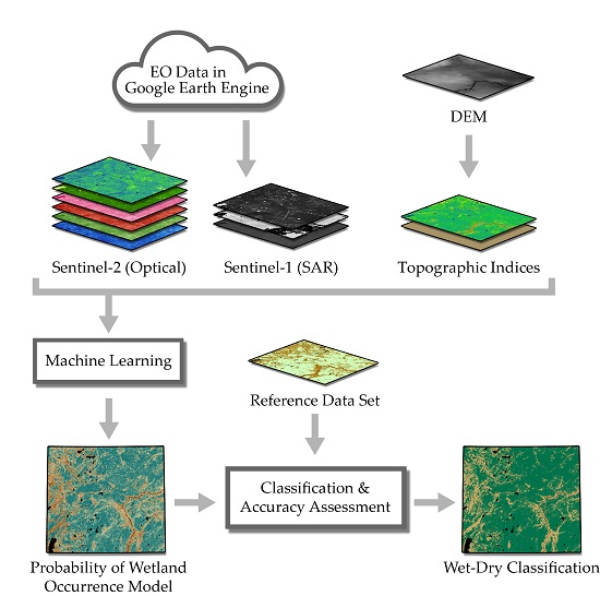
2. Materials and Methods

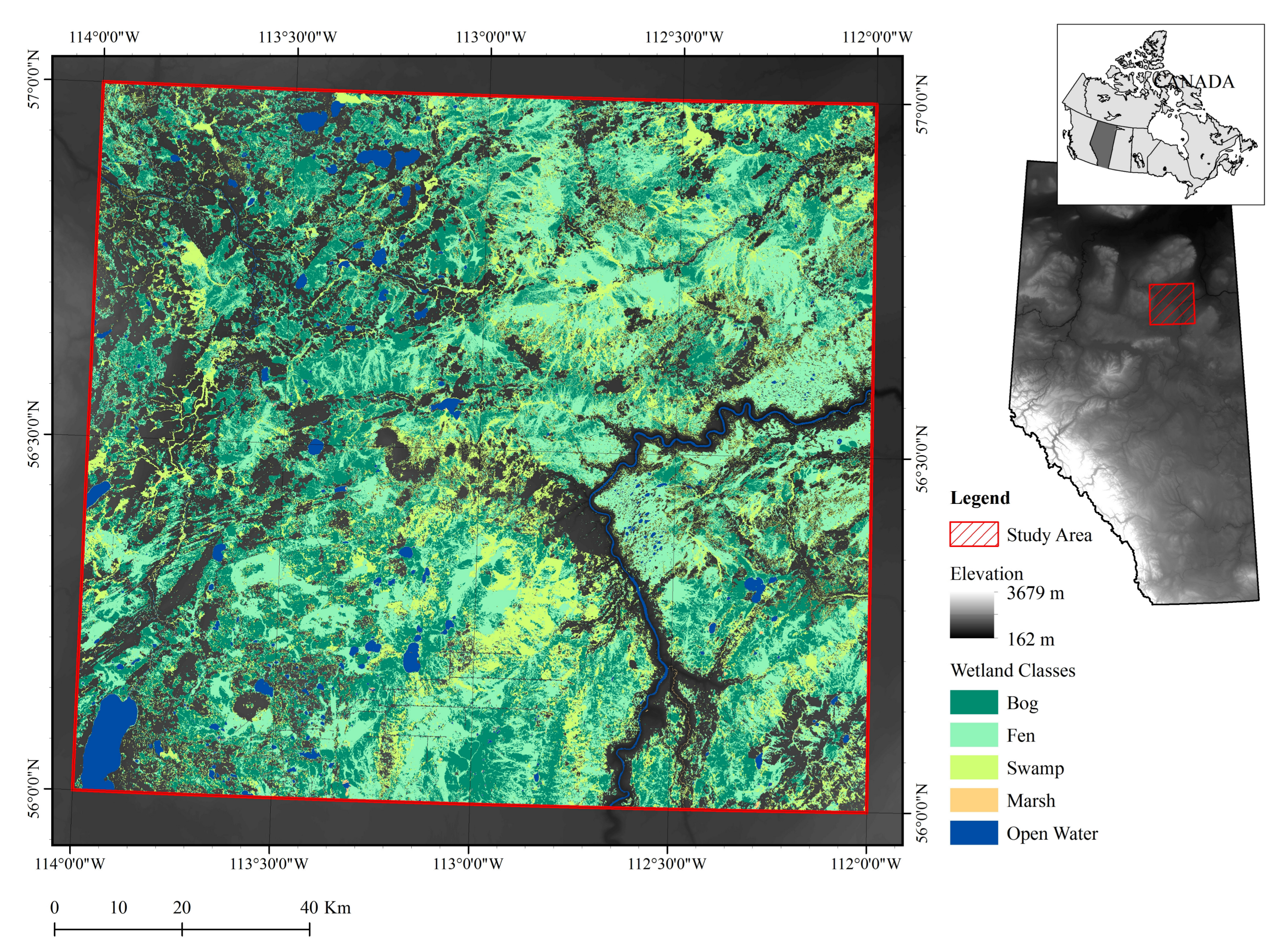
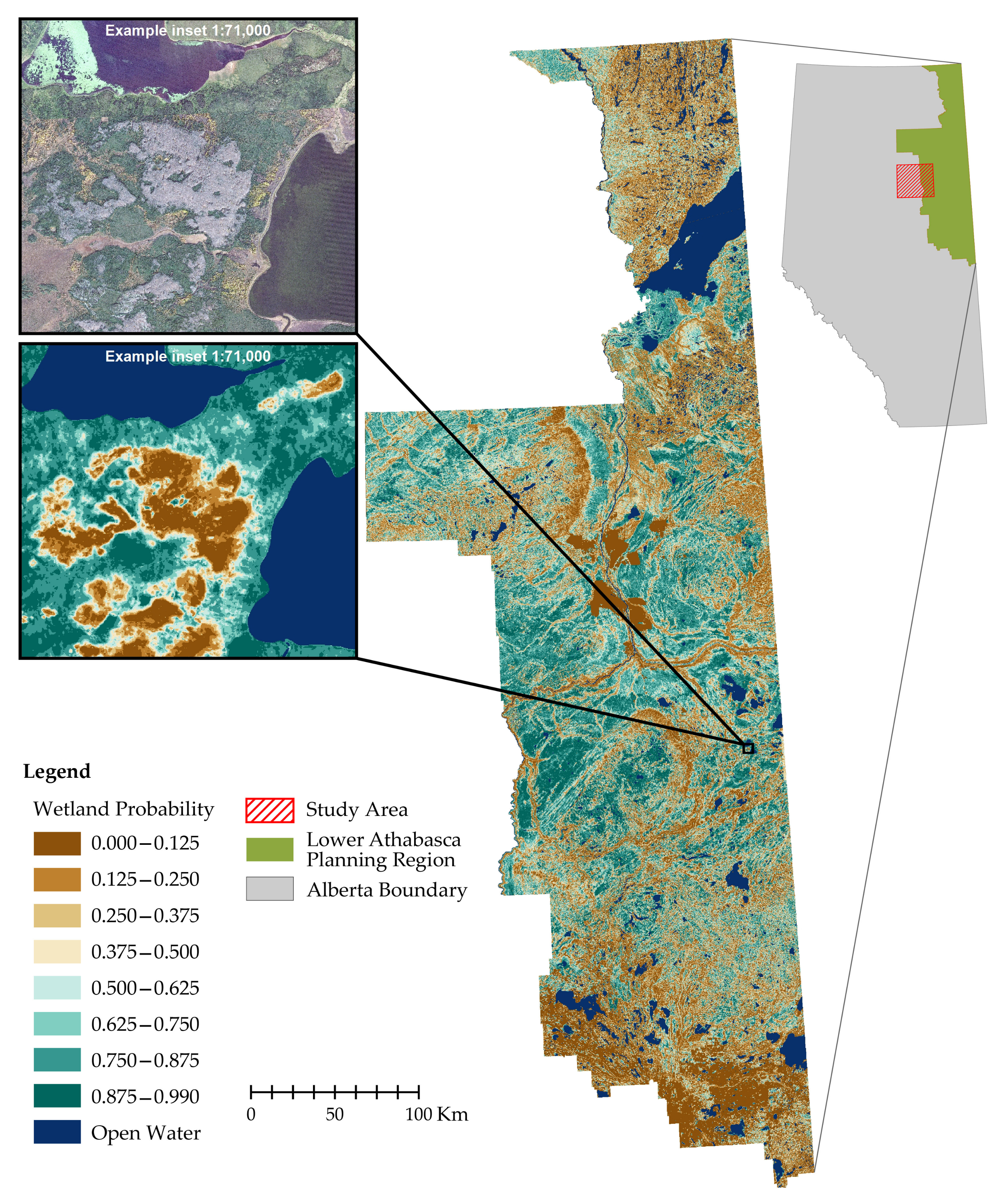
2.1. Study Area

Our case study area comprises a 13,700 km² region in northeastern Alberta, Canada, located within the Central Mixedwood Boreal Forest natural subregion (Figure 1). This subregion is characterized by flat to gently undulating plains containing extensive wetlands dominated by black spruce (Picea mariana (Mill.) Britton, Sterns & Poggenb.) fens and bogs (i.e., peatlands) [35]. Extensive peatland complexes—wetlands characterized by large accumulations of partially-decomposed organic peat below the surface [36]—are interspersed with hummocky uplands that typically support a mixture of aspen (Populus tremuloides Michx.), white spruce (Picea glauca (Moench) Voss), and jack pine (Pinus banksiana Lamb.) [35]. The Central Mixedwood climate experiences short, warm summers and long, cold winters. Elevation in the study area ranges from 286 m to 744 m above sea level.

Wetland dynamics within our study area are primarily hydrological in nature [37]. Inter- and intra-annual variability, particularly with regard to size, extent and local hydrological connectedness, is dominated by the timing and amount of seasonal precipitation, yearly meteorological variations, and longer-term climatic shifts [34]. Hydrological variation can be further influenced by land use changes such as forest harvest or the diversion of water resources for industrial or commercial use [38]. While our study area itself is in general relatively undisturbed, land use changes in upstream jurisdictions will have an effect on local hydrological dynamics.

2.2. Data Sets

Table 1. List and description of data sets included in the study, along with variables derived from each source.

Data Set	Description	Derived Variables
LiDAR (Light Detection and Ranging) Elevation	1-m LiDAR-derived Digital Terrain Model, combination of products based on LiDAR acquired between 2006 and 2010 by Airborne Imaging, provided by the Government of Alberta	Topographic Position Index (TPI), Topographic Wetness Index (TWI)
Optical Imagery	140 individual 10-m Sentinel-2 optical satellite images from May–August 2016 were acquired over the study area, provided by the European Space Agency	Blue (B2), Green (B3), Red (B4), Near Infrared (B8), Normalized Difference Vegetation Index (NDVI), Normalized Difference Water Index (NDWI)
Radar Imagery	37 individual 10-m Sentinel-1 polarimetric Synthetic Aperture Radar images were acquired over the study area; VV-VH (Pol) data was acquired May to August 2016, and VVsd and VV data were acquired April to October, 2014–2016, provided by the European Space Agency	Normalized Polarization (Pol), Vertical Polarization (VV), VV Standard Deviation (VVsd)
Reference Data	Vector polygon-based Alberta Vegetation Inventory Enhanced data, produced by aerial photograph manual interpretation, compiled and provided by the Government of Alberta *	Wetland—Non-Wetland Classification
Existing Wetland Inventory	Vector polygon-based Alberta Merged Wetland Inventory data, produced by Ducks Unlimited Canada using satellite image classification of imagery acquired between 1999 and 2002, provided by the Government of Alberta	Wetland—Non-Wetland Classification

* Note: Dates of aerial photography acquisition and interpretation on which this product is based, were unavailable from the source.

summarizes each of the data sets used in this study. They include a number of EO sources used to derive model-input variables, training data used in model building, reference data used to assess model performance and subsequent classification accuracy, and the existing wetland-inventory classification against which we compared our model classifications. A total of 177 satellite scenes were accessed and processed within the Google Earth Engine (GEE) environment [39]. Further details are provided in the following sections.

2.2.1. Topographic Data

We employed an airborne LiDAR (Light Detection and Ranging)-based digital terrain model (DTM) provided by the Government of Alberta’s Environment and Parks department to derive two input variables for modeling wetland probability of occurrence: topographic position index (TPI) and topographic wetness index (TWI). The data were acquired between 2006 and 2010 at densities of 1 to 4 points/m² using scan angles of less than 25° from nadir, and possess vertical accuracies of 30 cm or less root mean square error (per-data set accuracies). The 1-m digital terrain model (DTM) raster file was mean-aggregated to 10 m in order to match the spatial resolution of the Sentinel-1 and Sentinel-2 data. The TPI and TWI variables were computed for the study area using the System for Automated Geoscientific Analyses open-source software [40].

TPI represents the elevational position of each cell (i.e., pixel) in a DTM, relative to the average elevation of neighboring cells [41], whereby negative values indicate a particular cell to be lower than its surroundings (i.e., a valley) and positive values indicate the opposite (i.e., a ridge) [42]. TPI reflects local topographic positioning, and is therefore an important indicator of local low-lying areas or depressions, which are generally typical of wetland areas. This index is, however, scale-dependent, as the specified neighborhood within which it is calculated directly influences the resulting values [42]. Our TPI calculations followed Equation (1) [43,44], given as:

$$\mathrm{TPI}=Z_i-{\overline{Z}}_{R\left(i\right)}$$

(1)

Here, Z_i is the elevation of the ith pixel or cell, and ${\overline{Z}}_{R\left(i\right)}$ is the mean elevation of all cells within a given radius, R, of the ith cell. We employed a neighborhood radius of 100 m, which equals a window of 10 pixels by 10 pixels at our 10 m resolution. This scale was chosen as it was found, based on preliminary assessments, that TPI calculated using larger neighborhood sizes (e.g., 500 m) was more highly correlated to TWI than those calculated using smaller neighborhood sizes. A smaller neighborhood radius likely picks up the finer scale patterns of wetland occurrence, while TWI picked up the larger scale patterns of wetland occurrence. TPI values within our data ranged from −28.63 to 36.47.

TWI is considered as a proxy for the relative soil moisture of a particular cell [45]: a landscape attribute closely linked with wetland location and extent. TWI is calculated using Equation (2), taking slope, flow direction, and flow accumulation into account [42]. TWI was calculated using the following equation:

$$\mathrm{TWI}=ln\left(\frac{\alpha }{tan\beta }\right)$$

(2)

In the above, $\alpha$ is the upslope contributing area per unit contour, and $tan\beta$ is the local topographic gradient [26,46]. Higher TWI values indicate greater potential soil-water storage. In our study area, TWI values ranged from 0.13 to 10.81.

2.2.2. Optical Data

Optical variable inputs were derived from a series of 140 Sentinel-2A Level 1-C (top-of-atmosphere) satellite images that covered our study area, and were acquired on 24 separate dates between 15 May and 31 August 2016 (Table 1). A custom cloud-masking and compositing script written in JavaScript was used in GEE to remove various types of clouds and noise to produce a per-pixel, cloud-free, multi-spectral composite of the study area (code available in Document S1, provided in Supplementary Materials). The script first used Sentinel-2 Band QA60, a quality flag band [47], to identify and mask out flagged cloud and cirrus pixels. Remaining cloud and aerosols were then identified using Band 1, an aerosol band, and likewise masked. The latter was accomplished using a threshold of Band 1 ≥ 1500, selected on the basis of direct observation of B1 values within the images themselves. Both the normalized difference vegetation index (NDVI) and normalized difference water index (NDWI) were calculated for each Sentinel-2 image, using Equations (3) and (4) below [48,49].

$$\mathrm{NDVI}=\frac{NIR-Red}{NIR+Red}$$

(3)

$$\mathrm{NDWI}=\frac{Green-NIR}{Green+NIR}$$

(4)

Sentinel-2 Bands 4 and 8 were used for NIR and Red in calculating NDVI, while the NDWI’s NIR and Green variables were represented by Sentinel-2 Bands 3 and 8. Both of these indices produce values ranging from −1 to +1, and in our study area NDVI values ranged from −0.336 to 0.825, whereas NDWI values ranged from −0.315 to 0.797.

Finally, the GEE median-compositing function was used on the cloud-masked Sentinel-2 images to generate a per-pixel median composite of each of the multi-spectral bands and the two indices. This removed both dark pixels (e.g., due to shadow), as well as anomalously bright pixels (e.g., due to remaining cloud, haze or snow) from the resulting composite. Band 2 (blue), 3 (green), 4 (red), and 8 (near infrared), as well as NDVI and NDWI were extracted from the median composite, clipped to our study area, and exported from the GEE platform for use as model inputs.

NDVI is well-recognized and commonly-used in the remote sensing-based characterization of vegetation because of its sensitivity to photosynthetically active biomass and phenological dynamics in vegetation [50,51]. For this reason, we elected to include this popular index as one of our optical model inputs. The NDWI was selected as a complementary model input to the NDVI. Because of its sensitivity to open water [49], the NDWI has been included numerous times in wetland characterization as a means of detecting inundation or separating land from water (e.g., [52,53,54]).

2.2.3. Radar Data

Radar input variables were generated from a series of 37 Sentinel-1 synthetic aperture radar (SAR) C-band Level-1 Ground Range Detected images at a 10 m spatial resolution (Table 1). The data that were accessed through GEE included imagery from both ascending and descending orbits, and were collected using the Interferometric Wide swath mode, with average incidence angles ranging from 30° to 40°. The data were pre-processed using the Sentinel-1 Toolbox. The Toolbox applies thermal noise removal, radiometric calibration, and terrain correction [55].

The first SAR-derived model input parameter was a normalized polarization (Pol), calculated from all VV, VH (vertical-vertical and vertical-horizontal polarization) images captured by the Sentinel-1 satellites from 15 May to 31 August 2016. These were transformed using Equation (5) below, and subsequently smoothed using a 3 × 3-pixel mean filter (code available in Document S1, provided in Supplementary Materials).

$$\mathrm{Pol}=\frac{VH-VV}{VH+VV}$$

(5)

Here, VH represents a vertically transmitted, horizontally received SAR backscatter signal from the Sentinel-1 sensor, while VV represents a vertically transmitted and received SAR backscatter signal from the same sensor. Outputs from this index can theoretically range from −1 to +1, but in our study area they ranged from −0.048 to 0.999.

The Pol normalized index was selected for two reasons. First, the numerator (i.e., VH − VV) reflects the depolarization ratio described in [56]. Due to its sensitivity to surface roughness, as well as vegetation structure and dry biomass [57,58], it has proven useful for discriminating between bare and forested surfaces [59], and as an important input parameter in soil moisture retrieval [60]. Secondly, the normalization of the depolarization ratio replicates the microwave polarization difference index introduced in [61], which demonstrated sensitivities to vegetation canopy density and surface moisture. More recently, this index has shown valuable potential for improving SAR-based land-cover classification because of its responsive relationship with plant water content and soil moisture [62]. Normalizing the depolarization ratio also served to reduce potential outliers within the data.

The second and third SAR-based model input parameters were derived from series of VV-polarized images that included Sentinel-1 VV and VV, VH data products covering the study area for the years 2014–2016, for the months of April through October (i.e., ice-free months). These comprised per-pixel mean VV polarized backscatter (VVmean) and the standard deviation of VV (VVsd). Each was calculated on a pixel-by-pixel basis from the SAR VV image stack, and subsequently smoothed using a 3 × 3-pixel mean filter. Our final inputs ranged in values from −22.54 decibels (dB) to −0.39 dB for the VV backscatter, and from 0.5 to 9.5 for VVsd.

The primary reason VV polarization was selected in this work was its high level of availability. As a rule, the Sentinel-1 satellites only collect HH or HH, HV C-band SAR over polar or sea ice-covered regions, while VV or VV, VH is collected over all other observation regions [63]. Of the latter, VV observations far outnumbered the dual-pol observations in our study area, suggesting that VV-polarized backscatter would be the most reliable source of Sentinel-1 SAR in support of long-term wetland mapping and monitoring. C-band VV backscatter shows a sensitivity to soil moisture in open areas [36], and has proven useful both in discriminating different types of herbaceous or low, sparsely-vegetated land covers [64,65] and flooded from non-flooded areas [34,66]. Including VVsd alongside VVmean allowed us to capture local levels of backscatter variability, and provide an indication of surface dynamics in addition to overall VVmean backscatter.

2.2.4. Training and Reference Data

Our model training and accuracy assessment reference data were independently extracted from an enhanced version of the Alberta Vegetation Inventory (AVIE) provided by the Government of Alberta, which is a provincial-level inventory of Alberta’s forested regions generated by the manual interpretation of aerial photographs, using a set of government standards and protocols [67]. Moisture regime, captured within AVIE polygons, was used to create a binary wet vs. dry reference layer whereby wet or aquatic moisture regimes were designated as Wet, and remaining polygons designated as Dry. This vector layer was then rasterized to a 10 m spatial resolution matching the model input variables, using ESRI’s ArcGIS 10.3 software (ArcGIS 10.3, Esri, Redlands, CA, USA).

2.2.5. Other Data

The final data set involved in our analysis comprised the latest version of the AMWI [28]. These data were used for comparison purposes only: we compared the accuracy of the current AMWI that exists within our study, as far as it relates to the differentiation between wetland and non-wetland, to the accuracy of our wetland-occurrence model outputs. The AMWI was not used as a source for either training or reference data. The purpose of this exercise was to evaluate how machine-learning, cloud-computing approaches to wetland mapping applied to open-access satellite data archives compares to more traditional (and more labor- and computational hardware-intensive) remote-sensing approaches. If our new methods compared favorably to established techniques, then we would view this work as a potential foundation for Alberta-wide wetland mapping.

Within our study area, the AMWI was generated using a Ducks Unlimited Canada supervised image classification [68] involving Landsat 7 Thematic Mapper and RADARSAT-1 image inputs, as well as some ancillary data sets including a digital elevation model (DEM). The AMWI is provided as a vector polygon data set with five basic wetland classes: bog, fen, swamp, marsh, and open water. The data set was clipped to the study area, reclassified into Wet vs. Dry, and rasterized to a 10 m spatial resolution with ESRI’s ArcGIS 10.3 software.

2.3. Modeling and Evaluation

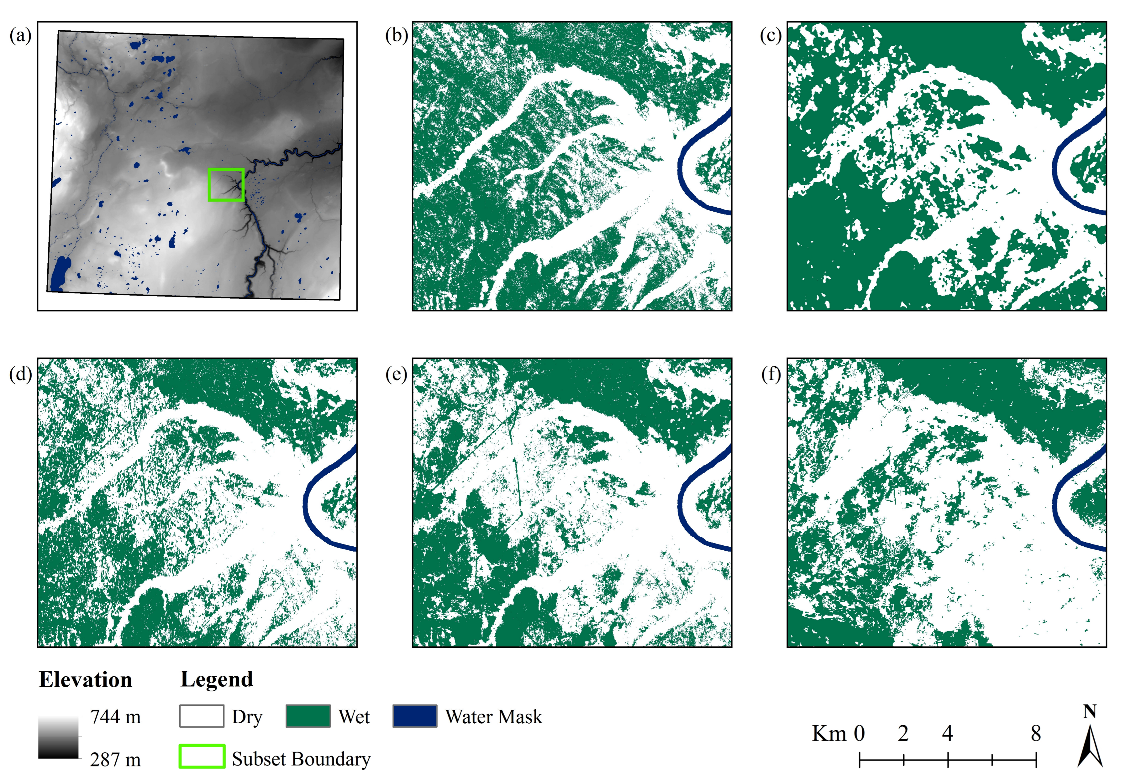
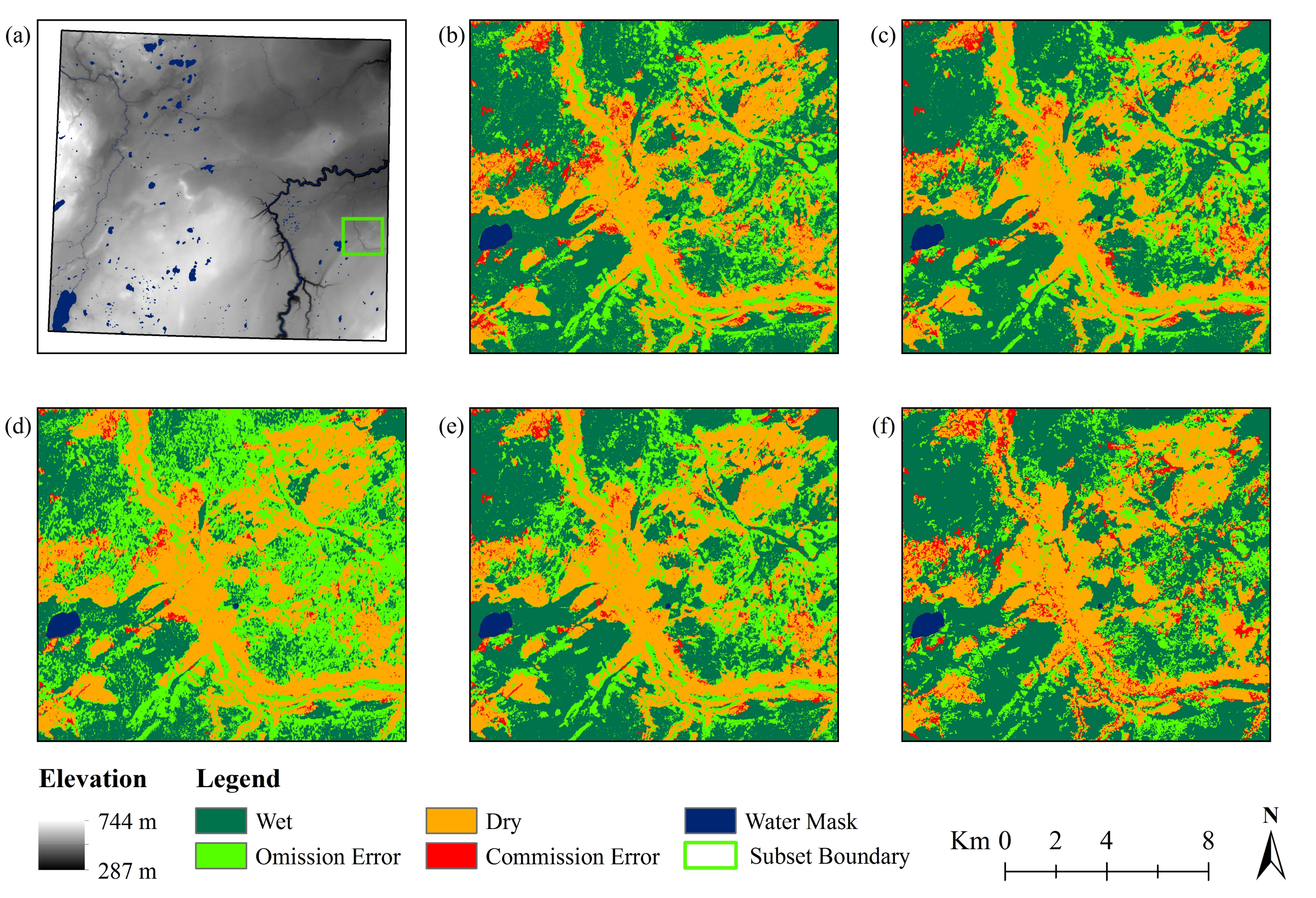
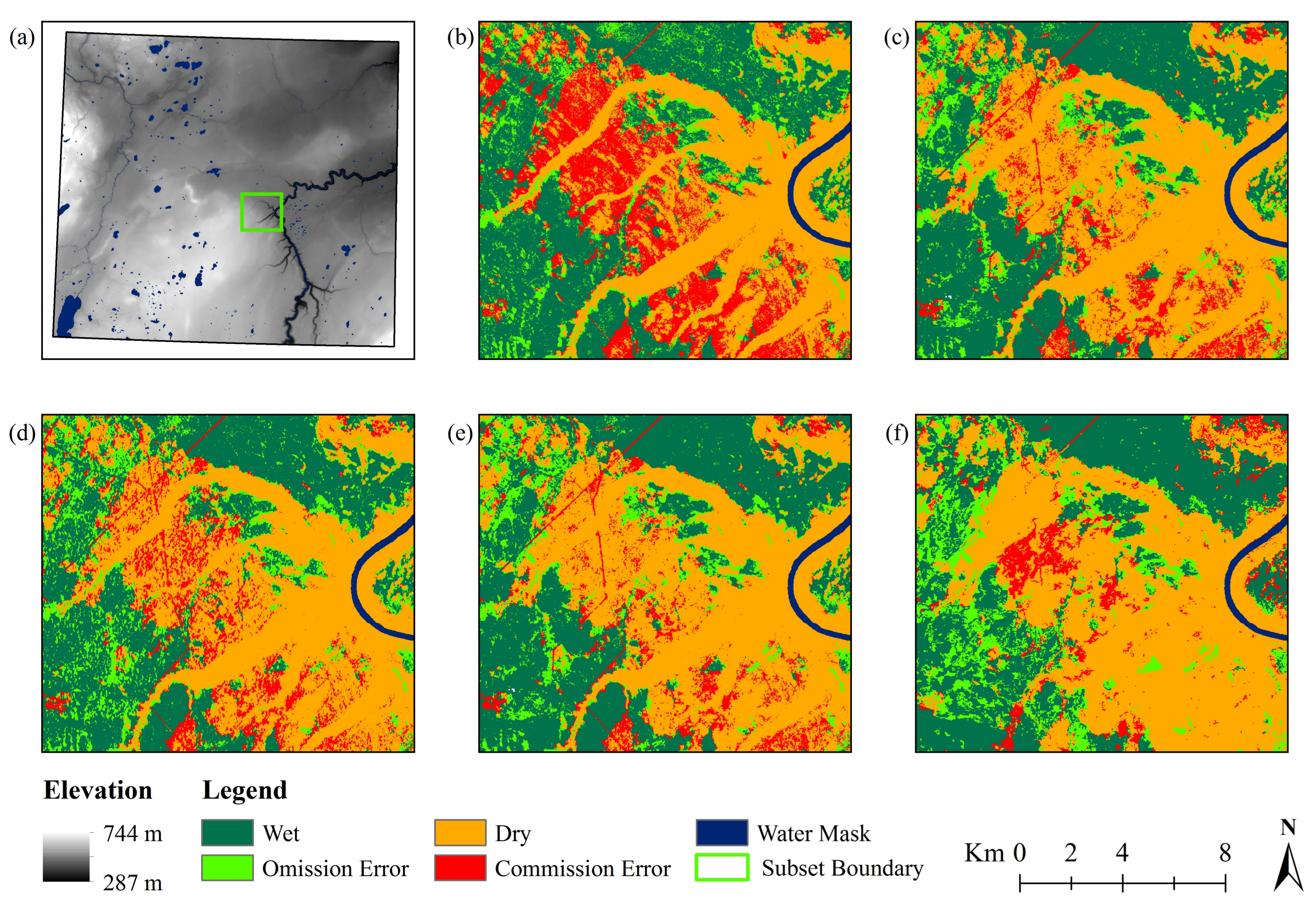
Probability of wetland occurrence was modeled using the boosted regression tree (BRT) machine-learning algorithm. BRTs adaptively generate numerous, simple regression-tree models and combine them into a multi-tree model, as a means of maximizing predictive performance while also providing insights into relevant variables and their interactions [69,70]. This contrasts with traditional regression approaches that produce a single predictive model. BRTs combine the ability of regression trees to accommodate all data types within a model, including missing or non-independent data, with the added advantages of boosting, that enables curvilinear functions to be modeled and increases robustness to data issues such as outliers [71]. A thorough, detailed description of BRTs is provided by [70].

Two important parameters are required for a BRT model: learning rate and tree complexity. The former establishes the contribution that each tree will make to the final model itself, while the latter indicates the number of nodes within each tree, and determines the number of variable interactions that are fitted [70]. A slower learning rate leads to a greater number of trees within a BRT model, since each tree contributes less to the overall model. However, greater numbers of trees require greater numbers of observations and computational time to build the model [70]. We selected a learning rate of 0.005 and tree complexity of 5, which lead to an average of 550 trees per model. An ensemble of 50 models was generated for each combination of inputs and then averaged as a means of producing a more robust, stable model by minimizing the inherent stochasticity that occurs in the individual models due to the subsampling and bagging that comprises the building of each tree [72]. Our bag fraction (i.e., the percent of data drawn at random, without replacement, from the full training set and used to build each tree in the BRT) was set to 0.5, based on information presented in [68]. Each model run involved a random sample of 200 points spaced at least 3.5 km apart. This reduced statistical overfitting and spatial autocorrelation between the sample points used to build each model, similar to what is described in [73]. A water mask, based on the Government of Alberta base features hydrological polygons (hereafter ‘Hydropoly’) water information was used to remove any known lake or river features from the sampling or modeling. Our data distribution parameter was set to ‘Bernoulli’ (i.e., logistic), to reflect the binary presence/absence nature of the training data.

Models were run within the R version 3.3.1 [74] statistical analysis environment, using the GBM package version 2.1.3 [75], along with additional customized code compiled by the authors (code available in Document S1, provided in Supplementary Materials). Four combinations of input variables yielded four BRT models: (i) topographic inputs (T_model); (ii) topographic and optical inputs (TO_model); (iii) topographic and SAR radar inputs (TS_model); and (iv) topographic, optical, and SAR radar inputs (TOS_model).

Model performance was evaluated using the area under the receiver operating characteristic curve (AUC) [76,77]—a powerful and commonly used measure of predictive model performance [78]—as well as explained deviance (D²). The latter is akin to variance reduction and is equivalent to calculating an R² when evaluating least-squares types of models [79]. It is calculated using the following equation:

$${\mathrm{D}}^2=\frac{D_{Null}-D_{Residual}}{D_{Null}}$$

(6)

where D_Null is the deviance of a model using the intercept only (i.e., no additional parameters), and D_Residual is the deviance that remains unexplained by this same model after all final parameters are included [79].

Additional model evaluation comprised thresholding each modeled wetland probability surface to produce a Wet-Dry binary classification, and conducting a traditional classification accuracy assessment on each. A threshold was selected using the true skill statistic (TSS), calculated for a series of possible classification thresholds (i.e., 0.05, 0.1, 0.15, …, 0.90, 0.95). Plotting TSS over a range of classification thresholds enables the selection of the threshold at which TSS, a measure of classification performance, is maximized.

The TSS, also known as the Hanssen-Kuipers discriminant, compares the number of correctly classified samples to that of a hypothetically perfect classification, while removing those correctly classified samples that could be attributed to chance agreement [80]. TSS is calculated using Equation (7) below, and offers a more objective measure of classification accuracy, similar to the kappa coefficient that is frequently used in the remote sensing literature [81]. However, the TSS is not influenced by class prevalence (i.e., the prevalence of particular classes within the area of interest) or by the size of the validation data set, as has been shown to be the case for the kappa coefficient [80].

$$\mathrm{TSS}=Sensitivity+Specificity-1$$

(7)

In this study, Sensitivity refers to the Wet class producer’s accuracy, while Specificity refers to the Dry class producer’s accuracy. These two terms originate from the ecological presence-absence distribution model literature (e.g., species and habitat distribution models; see [80] for examples), which are analogous to the probability-of-wetland-occurrence models produced here. Sensitivity is generally used to describe the proportion of observed presences (i.e., wetlands) that are correctly predicted as such, and is a measure of the level of omission errors [80]. Specificity, on the other hand, is a measure of errors of commission, representing the proportion of correctly predicted absences (i.e., non-wetland) [80].

Classification accuracy assessments involved the random selection of an independent set of 40,000 sample points, distributed across the study area, which once again was masked by the Government of Alberta Hydropoly information. Error matrices generated for each map supported the calculation of producer’s, user’s, and overall accuracies, as well as the TSS and kappa. The latter was included in our analysis both as a means of comparison with the TSS and overall accuracy, and because of its familiar use in remote sensing-based image classification evaluations. Errors of Wet class omission and commission were also mapped over the study area for each of our classifications, as a means of examining their spatial distributions.

A binary Wet-Dry classification derived from the AMWI was included in the above classification accuracy assessment analysis, as a means of comparing our models results with the existing wetland inventory over the study area.

3. Results

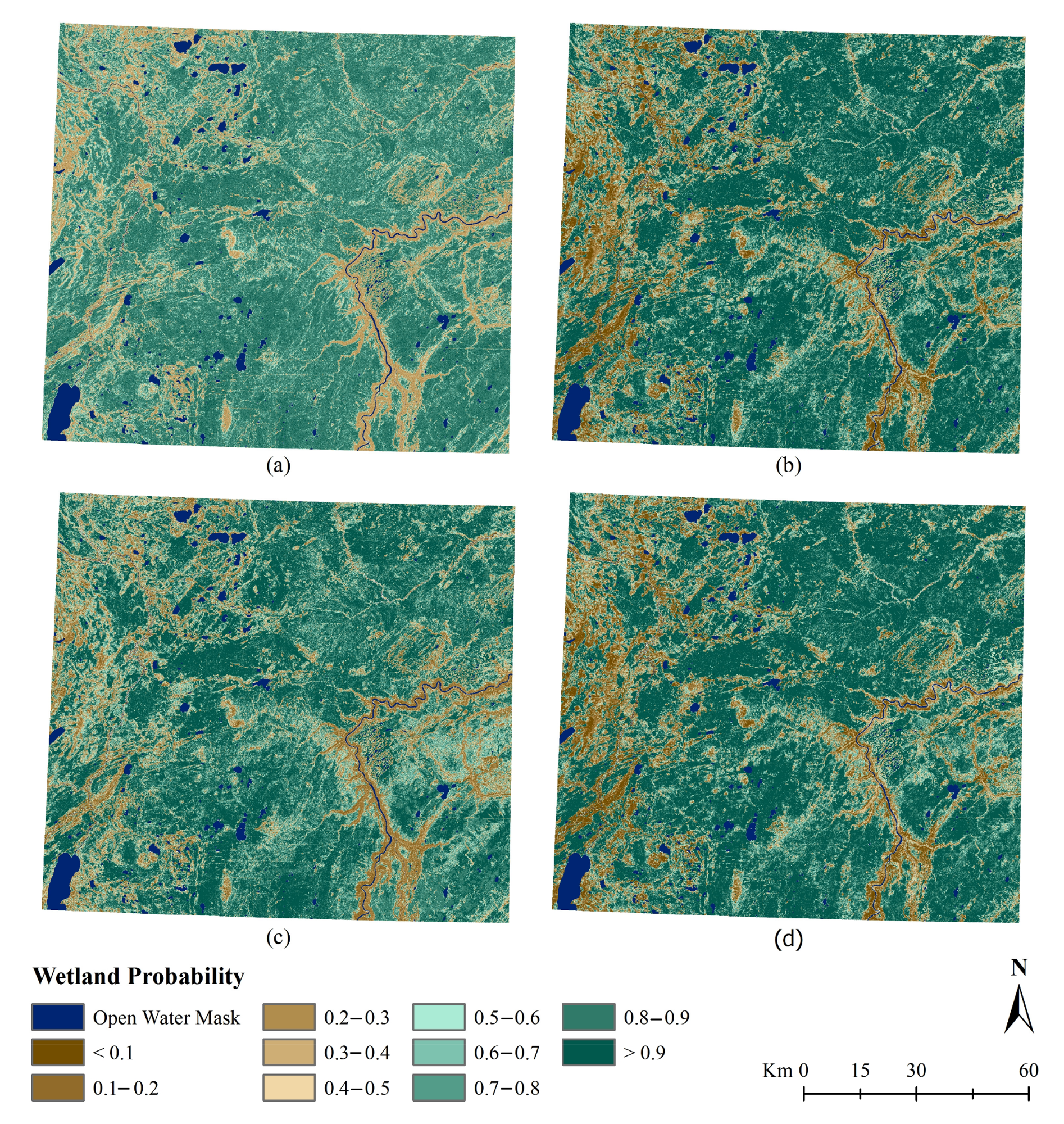
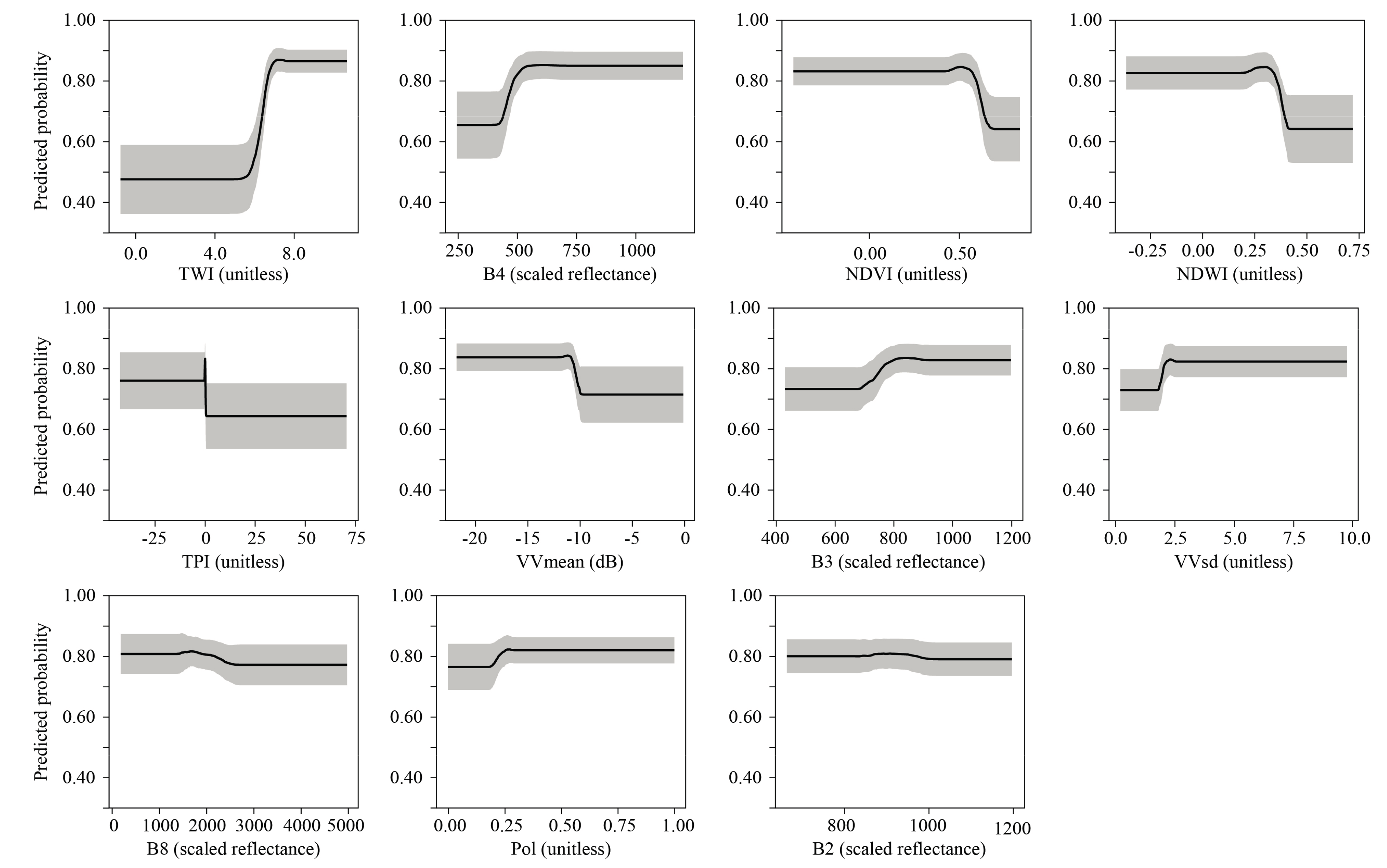
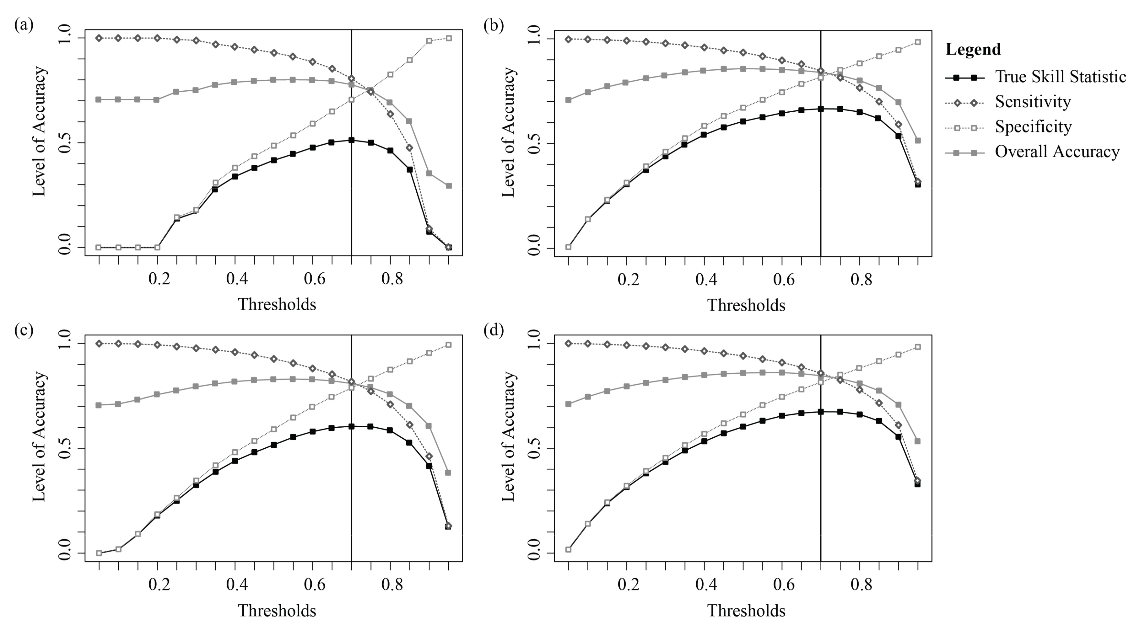
3.1. Probability Models

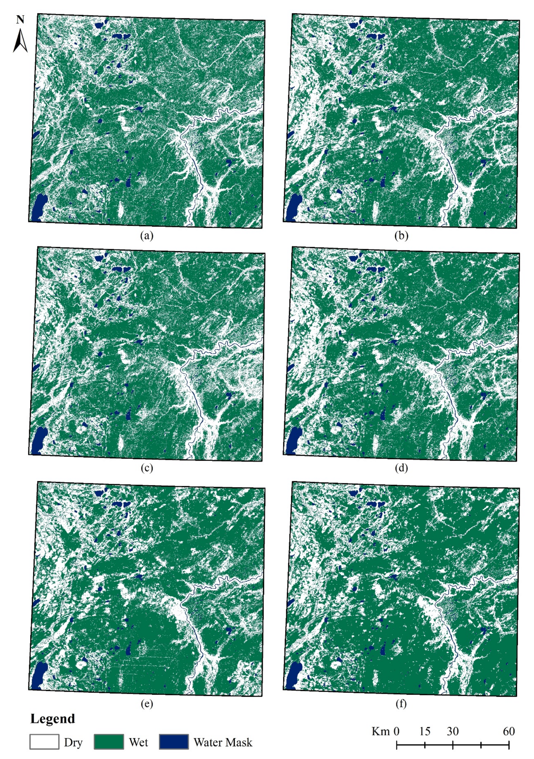
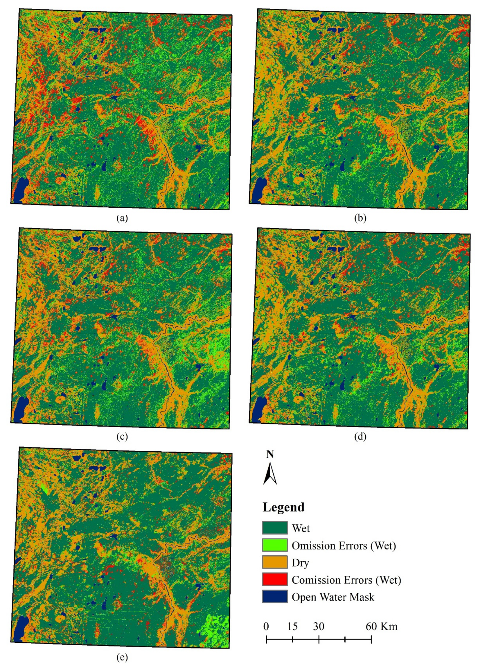
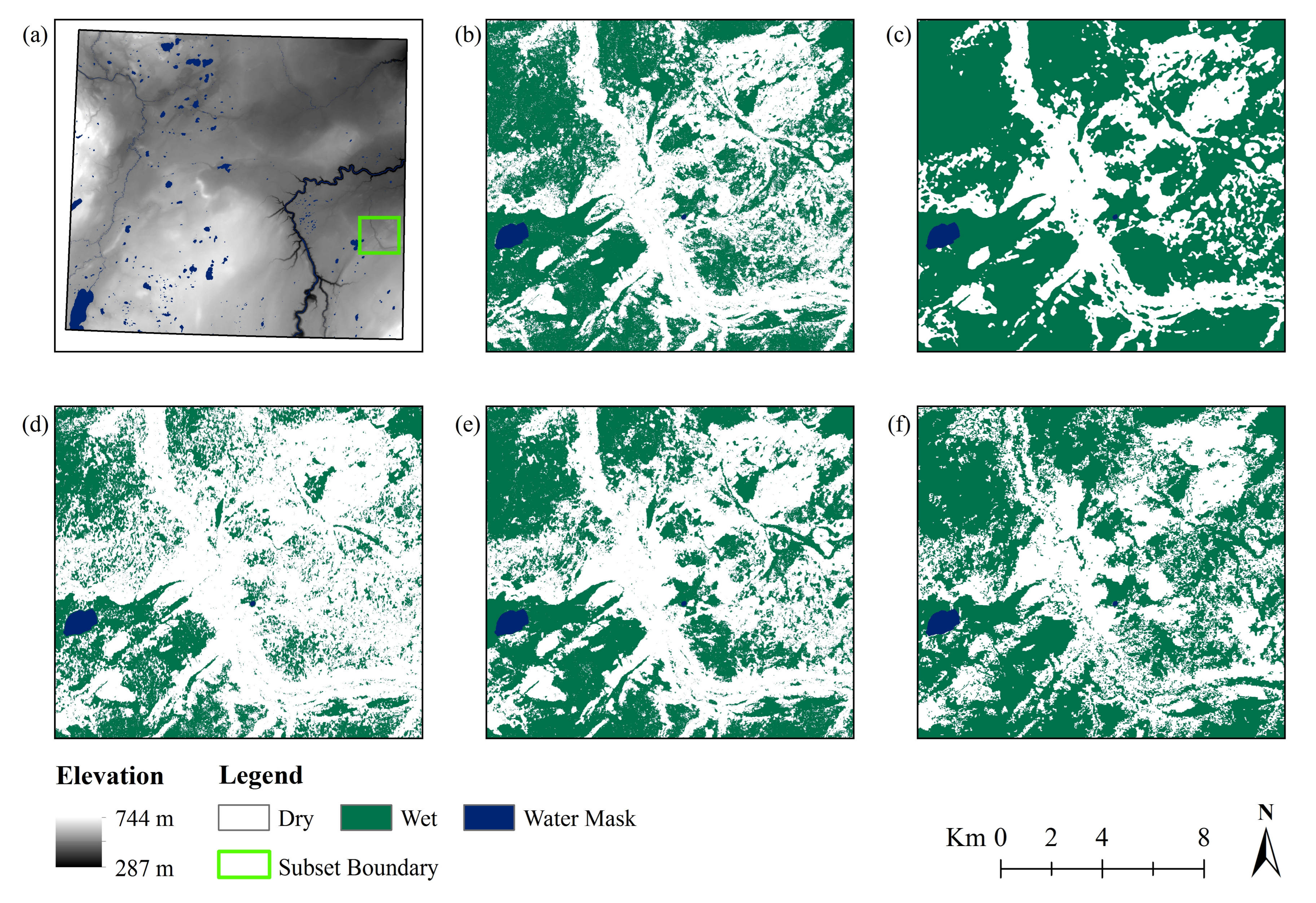
The outputs of the four probability-of-wetland-occurrence models are shown in Figure 2. Overall patterns in wetland probability and landscape features, such as river valleys and ridges of dry uplands, are comparable between the four models. The most noticeable qualitative difference between the models is the lack of very high and very low wetland probabilities in T_model probability surface, as are seen in the TO_model and TOS_model probability surfaces (Figure 2). The latter two are very similar in their results, while the TS_model and T_model are more distinct, particularly in the east-central portion of the study area where the TS_model produced areas of noticeably lower probability predictions.

Table 2. Receiver operator characteristic curve area under the curve (AUC), explained deviance (D²) model performance statistics, and number of trees per model averaged over the 50 iterations conducted per model; standard deviation between the 50 models shown in brackets.

Model	AUC	D2	No. of Trees
Tmodel	0.804 (0.037)	0.371 (0.061)	378 (100)
TOmodel	0.894 (0.026)	0.664 (0.069)	627 (154)
TSmodel	0.868 (0.027)	0.568 (0.065)	531 (105)
TOSmodel	0.898 (0.024)	0.708 (0.071)	671 (136)

lists the model-performance statistics calculated for each of the four models. All four produced good to excellent AUC statistics, with both the TO_model and TOS_model generating AUC values > 0.89, indicating high model accuracy [77]. Total deviance, a measure of model fit, decreased only slightly with the individual additions of optical and SAR inputs, respectively, but when combined into the TOS_model, offered a greater decrease in total deviance, which equates to an increase in model fit.

Relative variable importance for each model, averaged again over the 50 model iterations, are shown in Figure 3. Measures of relative variable importance or influence are calculated using the number of times a variable is selected for splitting within each regression tree, and the improvement this variable brings to the overall model each time it is selected [70]. In all four of our wetland probability models, TWI was the most influential predictor variable, followed by NDVI, NDWI, B4 and TPI in those models incorporating optical inputs, and by VVmean and TPI in those models incorporating SAR inputs.

The effect of each variable on a BRT model, after accounting for the average effects of all remaining variables in a model, can be visualized using the averaged partial-dependence plots [70]. Partial-dependence curves for TOS_model are given in Figure 4. Equivalent plots for the other three models are not provided here, because their partial-dependence functions show equivalent patterns for each set of input variables. Figure 4 shows that higher probabilities of wetland occurrence coincided with lower values of NDVI (<0.50), NDWI (<0.50), TPI (≤0) and VVmean (<−10), and higher values of TPI (≥0.7) and B4 (≥500). These six variables showed the most dramatic influence on wetland probability modeling, as seen in Figure 3.

3.2. Classification

Plotting model TSS, sensitivity, and specificity values over a series of possible classification thresholds resulted in selecting a 0.7 wetland-probability threshold for classifying the four probability model surfaces. This is the threshold at which TSS was maximized (Figure 5), and was also at or close to the threshold at which both sensitivity and specificity were balanced. Overall accuracy, also plotted in Figure 5, maximized around the 0.5 or 0.6 threshold.

Figure 6 presents the results of applying a 0.7 probability threshold to each of the four model probability surfaces to produce wetland classifications of the study area. The current AMWI and our AVIE reference data set are also shown in Figure 6. As with the model-probability surfaces, all six classifications show similar overall landscape-level patterns of wetlands, particularly around the river system in the southeastern corner of the study area. Local patterns between the models show notable variation, as seen in the example subsets (Figure 7 and Figure 8). In both examples, the TS_model produced the most noise in the resulting classification, and the least amount of Wet area. This contrasts with the TO_model classification, where the boundaries between the two classes are clearer, there is far less pixilation, and the model produces the greatest amount of Wet area within the subsets (Figure 7 and Figure 8). The T_model and TOS_model-derived classifications show local patterns in between the two extremes seen in the TO_model and TS_model classifications, while the AMWI classification appears most similar to that produced by TOS_model.

Table 3. Model and Alberta Merged Wetland Inventory (AMWI) classification accuracy measures, including class producer’s and user’s accuracies.

Classification	Overall Accuracy	True Skill Statistic	Kappa	Wet Producer’s Accuracy *	Wet User’s Accuracy	Dry Producer’s Accuracy **	Dry User’s Accuracy
Tmodel	0.777	0.513	0.489	0.807	0.868	0.706	0.603
TOmodel	0.840	0.666	0.633	0.848	0.918	0.818	0.692
TSmodel	0.809	0.604	0.568	0.818	0.902	0.786	0.642
TOSmodel	0.855	0.674	0.645	0.859	0.918	0.815	0.706
AMWI	0.854	0.672	0.656	0.878	0.911	0.794	0.731

* Equivalent to model sensitivity. ** Equivalent to model specificity.

lists the overall and classaccuracy measures calculated for each of the model classifications as well as the AMWI covering the study area. Overall accuracies range from 0.777 for the T_model classification to 0.855 for the TOS_model classification, while TSS measures range from 0.513 to 0.674 for these same classifications, respectively. Kappa statistics show a similar pattern again, but are highest for the AMWI. Similar to model performance, TOS_model and TO_model produce the highest classification accuracies of the four models, with the AMWI a close second behind TOS_model according to overall accuracy and TSS values. This same pattern can be seen in the producer’s and user’s accuracies for both classes, with the AMWI classification performing similarly to both models containing optical variable inputs, and performing slightly better in terms of Wet class producer’s accuracy and Dry class user’s accuracy (Table 3). Wet class accuracies are higher than those for the Dry class, in both producer’s and user’s accuracies.

The final portion of our analysis involved mapping errors of omission and commission for the Wet class: the class of interest. Figure 7 shows the full maps of these errors, again for all four model classifications and the AMWI. Overall landscape-level patterns of correctly-classified Wet and Dry pixels, as well as particular areas of omission or commission errors are similar between the four modeled classifications. The latter, in particular, are quite different in the AMWI classification (Figure 7).

When examined more closely, using the same subset areas shown in Figure 8 and Figure 9, local patterns of errors are more variable between the different classifications (Figure 10 and Figure 11). In particular, the TS_model classification shows a particularly high level of Wet class omission error, and relatively fewer errors of commission.

The other three model classification are quite similar to one another in their levels and patterns of error, particularly the T_model and TO_model classifications, with the TOS_model classification showing a slightly higher level of omission error and slightly lower level of commission error. The AMWI classification appears to show the least amount of omission error in this subset example, but equivalent levels of commission error.

Error patterns observed in Figure 11 are quite different from those in Figure 10. In the former, the T_model classification produced a notably higher number of commission errors, clustered in large patches within this subset example. In the four models, TOS_model produced the lowest level of commission error, while the AMWI produced an equivalent or slightly lower level of commission error in this example (Figure 11). Errors of omission are more similar between the four model classifications, but appear to be lowest in the T_model classification. This type of error appears highest in the AMWI, in this example.

4. Discussion

4.1. Modeling Wetland Occurrence

The results show that probability of wetland occurrence can be modeled with good success in Alberta’s northeastern boreal forest using topographic inputs and BRT machine learning models. An AUC statistic of 0.804 indicates strong discrimination between Wet and Dry areas with our model. Comparison with other models, as well as our reference data set, indicate that overall patterns of wetland distribution are well-captured within our study area. The TWI input variable was of greatest importance to our T_model (Figure 3), reflecting the importance of local topographic and hydrographic conditions in wetland occurrence: a relationship also demonstrated by other topographically-based wet areas mapping efforts such as those described by [82,83]. Indeed, the TWI showed the greatest influence of all input variables in each of the four probability models, regardless of what additional input variables were included (Figure 3). The TPI was also important in model development, though to a lesser extent.

Converting T_model into a map of Wet and Dry classes using a threshold of 0.7 yielded a classification with moderate accuracy, once random chance was factored into the assessment (TSS = 0.513; Table 3). Errors of omission and commission for the Wet class can be calculated from Table 3 as 19.3% and 13.2%, respectively, indicating that more than 80% of actual Wet areas according to the reference data set are captured by the Wet class, and more than 85% of Wet class pixels in the produced map represent actual Wet areas. Our results are encouraging for the future application of this approach to mapping wetlands across the province of Alberta, as 84% of the province now has LiDAR coverage.

Commission errors in the T_model classification are slightly concerning, as they show notably clustered patterns in the error map shown in Figure 7, and also seen in Figure 11. This pattern indicates that the TWI and TPI input variables do not explain wetland occurrence under particular conditions found within these patch-like portions of our study area. A closer examination of these two topographic input surfaces in the subset found in Figure 11 reveal that neither variable shows great distinction between the areas identified as commission errors and the nearby correctly identified Wet areas. In these areas, is appears that there are additional factors at play which are not being captured by the topographic inputs in T_model; perhaps reflecting variations in other characteristics such as soil properties or vegetation communities. Indeed, as noted earlier, both [33,34] observed that the glaciated substrata that underlie Alberta’s boreal plains lead to intricate and highly variable ground-surface water interactions, and that these interactions are not always reflected accurately by local topography alone. Subsurface soil information is an important factor which contributes to the current distribution of wetlands [36], is not captured with our current methods. Topography is an important component of wetland distribution in this ecozone, but not the single driving factor.

In addition to the above-noted limitations, it is important to acknowledge that the choice of neighborhood size used in calculating the TPI is likely a source of further uncertainty in this work. While our 100 m neighborhood radius appeared to work well for our study area, it is arbitrary and may not be the most optimal. Further work is recommended in order to better examine the effects of radius size in TPI calculations on wetland occurrence mapping in our study area. A multi-resolution TPI or multiple scales of TPI may offer a better approach to using relative elevation information in future wetland modeling work.

Despite its limitations, the performance of our topographically based BRT model is comparable to other similar modeling approaches described in the literature. For instance, both [32,84] employed various topographic inputs, including TWI, within predictive classification and regression trees (CARTs) modeling approaches to delineate wetland boundaries in southern Ontario, Canada, though each study employed a different topographic data source. The CART models in both studies produced overall classification accuracies of 84% [32,84], which is slightly higher than our T_model accuracy of 78% (Table 3). In contrast to these studies, Kasischke E.S. et al. [85] employed the TPI derived from a LiDAR DEM covering a study area in eastern Florida, U.S.A., to identify small depressional wetlands that are of great importance to local amphibian species. Their wetland overall classification accuracies ranged between 67% and 81% for depressional wetlands of different hydroperiod classes, demonstrating the usefulness of the TPI in identifying these types of small wetlands that are rarely captured within broad wetland inventories [85].

It is also worth noting that the source of our training and reference data sets itself—the AVIE—is not perfect and contains misclassification errors. These data are generated through air-photo interpretation, and therefore are likely not able to capture underlying topography and hydrologic regimes perfectly, particularly in densely forested areas where treed fens or swamps may be misinterpreted as upland areas. This highlights one advantage of the topographic approach to modeling wetland occurrence.

4.2. The Value of Optical and SAR Inputs

Including optical and SAR input variables, or both, into our BRT models of wetland probability of occurrence improved model performance from an AUC statistic of 0.804 to 0.894, 0.868, or 0.898, respectively (Table 2). Including optical input variables improved the model to a greater degree than including SAR input variables, suggesting that the optical data was more important for increasing model predictive power than SAR data. This is supported by the observation that including SAR variables along with optical variables does not further improve the model by a large amount. TO_model and TOS_model performed very similarly in all of our analyses, though the latter slightly out-performed the former. Further evidence can be found in the relative variable importance measures calculated for each of the four probability models. In the TOS_model, SAR input variables were less important to model development than both of the topographic input variables, and three of the optical input variables—i.e., red reflectance (B4), NDVI and NDWI (Figure 3). With regard to classification-accuracy measures, this same pattern is again observed: the addition of optical input variables provided a larger increase in accuracy than SAR input variables, according to all calculated statistics, including both producer’s and user’s accuracies (Table 3). This trend might suggest that the variations in overall vegetative productivity reflected by B4 and NDVI inputs, and the contrast between dry and wet surfaces captured by the NDWI are more reflective of wetland occurrence in our study area than the soil moisture or surface roughness represented by our SAR model inputs.

We acknowledge that our particular SAR-derived model inputs are relatively simple in nature, and limited by the availability of particular polarizations provided by the Sentinel-1 sensors. It has been shown in the literature that both VH- and HH-polarized backscatter can outperform backscatter in the VV polarization with regard to detecting plant density [57], extracting flooded forests [86], and general wetland type discrimination [65]. However, C-band HH backscatter is not currently collected over terrestrial mid-latitudes by the Sentinel-1 satellites.

In addition to alternative polarizations, further exploration into more sophisticated SAR-based information products such as decomposition techniques for extracting scattering mechanisms would be worthwhile as a means of gaining a deeper understanding of the role that SAR data could play in a modeling approach such as ours, even though our goal was prediction rather than inference (i.e., understanding the Earth processes behind the model itself).

It is also important to note that seasonal and moisture dynamics play a key role in the use of SAR and optical data for modeling wetland occurrence: local meteorological conditions present during the time of acquisition will impact model results. In our case, weather records show that in comparison to Environment Canada’s 1981–2010 climate normal [87], both 2014 and 2015 were drier than average in our study area, particularly during the latter year when precipitation was below normal for much of the year [88]. In 2014, both spring and fall precipitation were higher than normal, but lower during the summer months [88]. However, 2016 showed higher-than-normal precipitation over both the summer and fall, particularly in July. With regard to temperature, all three years were slightly above normal, particularly in the summer months [88]. Our Pol variable is calculated using only 2016 summer data, because of the limited availability of VH-polarized data. This variable is thus likely to be particularly affected by the wetter-than-normal conditions that were present that year, and may introduce a bias toward the over-estimation of wetland occurrence. However, our VVmean and VVsd inputs were calculated using data from spring, summer and fall for all three years, and thus reflect both wet and dry conditions, which were of greater importance in our models than the Pol variable (Figure 3).

Despite the superior performance of optical inputs in our models, it is worth noting that including either optical or SAR variable inputs into our models did improve the model's ability to more correctly discriminate most of the patches of commission errors observed in the error map for TOS_model. This is particularly evident in Figure 11.

Evaluating the increase in model performance or classification accuracy offered by adding optical or radar input variables to a topographically-based wetland mapping approach is unique; in general, the literature describes studies evaluating the reverse. Optical and radar satellite data sets are more widely employed in mapping wetlands, likely because these data sets have typically been more readily available in the past, while high-quality topographic data sets, such as those derived from LiDAR, have often been geographically limited or inaccessible for proprietary reasons. Nevertheless, as high-quality LiDAR- or satellite-based topographic data sets become more common and more accessible in many jurisdictions, they are able to support broader applications of wetland modeling and mapping.

4.3. Towards Alberta-Wide Mapping

The best probability-of-wetland-occurrence model—TOS_model—produced a Wet-Dry classification with a level of accuracy very similar to that yielded by the AMWI that currently exists within the study area. This indicates that the BRT modeling approach described here can produce a Wet-Dry map product equivalent to the wetland inventory that is currently employed by the Government of Alberta. It must be recognized that the AMWI is far more than a simple binary wetland classification: it provides information on the distribution of several different hierarchical wetland types. However, for the purposes of this study, its value as a map of wetland location and extent only, was evaluated here.

Despite the comparable classification accuracies between our BRT models and the AMWI, each is produced using very different approaches that involve disparate levels of effort and resources. The AMWI segment that covers our study area incorporates Landsat and RADARSAT imagery, along with a number of ancillary data sets that included topography as well as forest inventory and fire history data, into an object-based image segmentation, and rule-based, supervised classification approach [68]. The procedure used to produce this particular portion of the AMWI required significant levels of user involvement, data preparation, statistical analysis, and manual editing within a multi-tiered workflow that would be challenging to reproduce on a regular basis in order to update the product [68]. In addition, at least some of the ancillary data involved in producing the AMWI over our study area is unlikely to be widely-available or recently updated (e.g., local forest inventory information), further limiting the updatability of the AMWI product. It should be noted that other amalgamated components of the AMWI were generated using alternate data sets and methods, which vary from region to region, rendering different portions of this dataset easier or more difficult to update. For instance, the AMWI in alternate regions of Alberta comprise both satellite- and air photo-based manual interpretation, which are themselves far more costly and time-consuming than computerized image classification methods like the one described here.

In contrast to the AMWI, our BRT modeling approach involves widely available remotely sensed data sets, and at least with regard to our Sentinel-1 and -2 radar and optical inputs, data that is regularly updated and freely accessible through online digital satellite data archives (e.g., through the European Space Agency). In addition, these data are offered in higher spatial (and temporal) resolutions, resulting in a classification at a 10 m resolution rather than a Landsat-based 30 m resolution for the AMWI. This represents 9-fold increase in spatial detail—a valuable characteristic that enables more a more detailed look at local wetland patterns.

The LiDAR DTM used in this study is proprietary data, and accessible only through data-sharing agreements with the Government of Alberta, but could readily be employed by government researchers, agencies, or contractors for the purpose of producing a consistent and comprehensive provincial-level wetland occurrence map. Another advantage of the BRT model approach is that satellite data access and pre-processing is done through an online cloud-computing platform (i.e., Google Earth Engine) that minimizes the amount of data downloading requirements or local desktop computer processing time and effort [3]. Finally, BRT models themselves can be run using free, open-source programming code packages such as R [74], which are easily modified to suit user needs, and highly adaptable to different model inputs as they are unaffected by data type, data gaps, or outliers [70].

The advantages of the BRT wetland-probability modeling approach described in this study for producing a regional-level (i.e., Alberta-wide) map of wetland occurrence, particularly in comparison to the existing AMWI, are clear. The approach, as described here, however, does possess some limitations that must be considered before being applied province-wide. First, the LiDAR DTM data set employed here does not quite cover the entire province of Alberta; it is available over much of the province with the exception of the Canadian National Parks and portions of the far north. Application of BRT models over these regions would require an alternate source of elevation data, such as NASA’s Shuttle Radar Topography Mission satellite or Japan’s Advanced Land Observing Satellite, both of which provide freely available, global elevation data sets. The effect of including topographic inputs derived from these types of data sets on BRT wetland probability models would need to be assessed.

A second limitation we acknowledge is that our approach does itself rely on out-of-date or infrequently updated data for model training and validation (i.e., AVIE; see Table 1). This is a recognized limitation that hinders consistent, repeated wetland occurrence modeling over time. However, it is one we hope can be addressed through the use of alternative data sets such as the Alberta Biodiversity Monitoring Institute’s detailed, air photo interpretation-based ‘photo-plot’ data [89,90]. The latter comprise a series of 3 km by 7 km areas distributed across the province that are being mapped for land cover and land use, and are intended to be kept relatively current over time. These would provide an open source more up-to-date source of reliable information on local wetland extents that could be used to inform larger-scale models.

A third limitation to the modeling approach described here is its current incomplete use of cloud-computing services, and reliance on desktop computer power to run the BRT models. Ideally, the modeling would be run within the same environment where the satellite data are pre-processed—Google Earth Engine—or a similar cloud-computing service offering similar levels of access to Sentinel data sets. GEE does currently provide machine-learning algorithms such as random forests, but these do not provide the flexibility that is currently offered within the BRT R functions. Fourth, we must recognize that the current study was conducted in only one of Alberta’s many different ecoregions: the boreal forest. Alberta itself is a very diverse province, comprising prairies, parklands, foothills, mountains, and various types of forested landscapes [35]. It is not known how well the current approach will perform over these different environments, and requires further work in order to assess this before it can be used on a fully operational scale to map wetland location and extent across the province.

In addition to the above limitations, we would be remiss if we did not also acknowledge additional sources of uncertainty that may reside with our satellite data sets. While we performed cloud and shadow removal on Sentinel-2 top-of-atmosphere reflectance, bidirectional reflectance effects from changing sun-sensor-surface geometries between acquisitions will remain, as will the effects of phenological variation in vegetation reflectance over the period of acquisition. Further processing of these data to bottom-of-atmosphere surface reflectance would be ideal. The European Space Agency does offer a Sentinel-2 processing toolbox for just this purpose [91]; however, as far as the authors are aware, this toolbox is only available as a local application and not yet implementable on a cloud-based platform. Its use for large-scale, multi-annual Sentinal-2 data sets is limited and for this reason, was not part of our workflow. It appears that GEE is moving towards implementing bottom-of-atmosphere Sentinel-2 imagery into its collection, but this was not available at the time of our study. Future studies using similar methods should aim to use the bottom-of-atmosphere products, if available. At present we believe our production of annual composites of optical input variables will suffice to minimize bidirectional effects to an acceptable degree. We also believe this annual compositing will have reduced much of the seasonal variation present in our optical data resulting from phenological variations in surface vegetation, as the former is designed to represent overall annual vegetative condition.

Despite the stated uncertainties and limitations of our approach to modeling wetland probability of occurrence, as proof of the approach’s scalability, we were able to apply TOS_model to a large portion of northeastern Alberta known provincially as the Lower Athabasca Planning Region (Figure 12), with good success. In generating this 93,213-km² information product, we processed 118 Sentinel-1 and 463 Sentinel-2 scenes in GEE. Our model produced a wetland classification accuracy of 80% (Kappa = 0.60), compared to an accuracy of 75% (Kappa = 0.51) for the equivalent existing AMWI over the same region.

Our results, and the subsequent successful upscaling of our BRT model to a much larger portion of the province demonstrate the advantages of exploiting current, freely available EO-data archives, supported by the cloud computing-based compilation and processing of said data sets, and the use of complex, machine-learning algorithms for large-area mapping and monitoring of wetlands. With our approach, regular, consistent province-wide mapping that can support the Alberta Wetland Policy and the responsible, sustainable management of the province’s wetland resources is much closer to full realization than a decade ago.

5. Conclusions

We demonstrated the successful application of a BRT modeling approach involving topographic variables to mapping wetland probability of occurrence across a portion of the Alberta boreal forest. Additional satellite-based optical variable inputs increased model performance and the accuracies of resulting wetland classifications. The further addition of satellite-based SAR input variables to topographical and optical inputs produced the best-performing model and classification, although optical data was found to increase model performance more than SAR data. The best BRT model produced classification accuracies comparable to the existing AMWI data of the study area, but requires fewer input data sets, less overall effort to produce, and is offered at a 10 m rather than 30 m spatial resolution. The BRT approach is also more easily updatable and expandable to broader regions than the AMWI. The TOS_model, when applied over a large area (the Lower Athabasca Region) in fact showed superior results to the equivalent the AMWI data set over the same region (80% accuracy versus 75%). Recognized limitations include the need to investigate the use of alternative topographic data sets where government LiDAR data do not yet exist, and the expanded use of cloud-computing services to incorporate more of the modeling workflow, therefore better enabling large-scale use. Nevertheless, the proposed approach presents a novel and promising technique for the future production of a consistent and comprehensive Alberta-wide wetland inventory product that can support long-term natural resource management policy development and regional planning within the province by taking advantage of recent technological advances and trends in the geospatial sciences.

References

1. Woodcock, C.; Allen, R.; Anderson, M.; Belward, A.; Bindschadler, R.; Cohen, W.; Gao, F.; Goward, S.N.; Helder, D.; Helmer, E.; et al. Free access to landsat imagery. Science 2008, 320, 1011–1012. [Google Scholar] [CrossRef] [PubMed]
2. Drusch, M.; Del Bello, U.; Carlier, S.; Colin, O.; Fernandez, V.; Gascon, F.; Hoersch, B.; Isola, C.; Laberinti, P.; Martimort, P.; et al. Sentinel-2: ESA’s optical high-resolution mission for GMES operational services. Remote Sens. Environ. 2012, 120, 25–36. [Google Scholar] [CrossRef]
3. Google. A Planetary-Scale Platform for Earth Science Data & Analysis. Available online: https://earthengine.google.com/ (accessed on 29 May 2017).
4. National Aeronautics and Space Administration Welcome to the NASA Earth Exchange (NEX). Available online: https://nex.nasa.gov/nex/ (accessed on 12 September 2016).
5. Amazon Web Services Inc. Earth on AWS: Build Planetary-Scale Applications in the Cloud with Open Geospatial Data. Available online: https://aws.amazon.com/earth/ (accessed on 28 November 2017).
6. Chandrashekar, S. Announcing Real-Time Geospatial Analytics in Azure Stream Analytics. Available online: https://azure.microsoft.com/en-us/blog/announcing-real-time-geospatial-analytics-in-azure-stream-analytics/ (accessed on 12 September 2017).
7. Yang, C.; Yu, M.; Hu, F.; Jiang, Y.; Li, Y. Utilizing Cloud Computing to address big geospatial data challenges. Comput. Environ. Urban Syst. 2017, 61, 120–128. [Google Scholar] [CrossRef]
8. Warren, M.S.; Brumby, S.P.; Skillman, S.W.; Kelton, T.; Wohlberg, B.; Mathis, M.; Chartrand, R.; Keisler, R.; Johnson, M. Seeing the Earth in the Cloud: Processing one petabyte of satellite imagery in one day. In Proceedings of the 2015 IEEE Applied Imagery Pattern Recognition Workshop (AIPR), Washington, DC, USA, 13–15 October 2015. [Google Scholar]
9. Hansen, M.C.C.; Potapov, P.V.; Moore, R.; Hancher, M.; Turubanova, S.A.A.; Tyukavina, A.; Thau, D.; Stehman, S.V.V.; Goetz, S.J.J.; Loveland, T.R.R.; et al. High-resolution global maps of 21st-century forest cover change. Science 2013, 342, 850–854. [Google Scholar] [CrossRef] [PubMed]
10. Pekel, J.-F.; Cottam, A.; Gorelick, N.; Belward, A.S. High-resolution mapping of global surface water and its long-term changes. Nature 2016, 540, 418–422. [Google Scholar] [CrossRef] [PubMed]
11. Yamazaki, D.; Trigg, M.A. The dynamics of Earth’s surface water. Nature 2016, 540, 348–349. [Google Scholar] [CrossRef] [PubMed]
12. DeLancey, E.R.; Kariyeva, J.; Cranston, J.; Brisco, B. Monitoring hydro temporal variability in Alberta, Canada with multi-temporal Sentinel-1 SAR data. Can. J. Remote Sens. 2017, in press. [Google Scholar]
13. Moody, D.I.; Warren, M.S.; Skillman, S.W.; Chartrand, R.; Brumby, S.P.; Keisler, R.; Kelton, T.; Mathis, M. Building a living Atlas of the earth in the cloud. In Proceedings of the 50th Asilomar Conference on Signals, Systems and Computers, Pacific Grove, CA, USA, 6–9 November 2016; pp. 1273–1277. [Google Scholar]
14. Goldblatt, R.; You, W.; Hanson, G.; Khandelwal, A.K. Detecting the boundaries of urban areas in India: A dataset for pixel-based image classification in google earth engine. Remote Sens. 2016, 8, 634. [Google Scholar] [CrossRef]
15. Zhou, L.; Chen, N.; Chen, Z.; Xing, C. ROSCC: An efficient remote sensing observation-sharing method based on cloud computing for soil moisture mapping in precision agriculture. IEEE J. Sel. Top. Appl. Earth Obs. Remote Sens. 2016, 9, 5588–5598. [Google Scholar] [CrossRef]
16. Huntington, J.L.; Hegewisch, K.C.; Daudert, B.; Morton, C.G.; Abatzoglou, J.T.; McEvoy, D.J.; Erickson, T. Climate Engine: Cloud computing and visualization of climate and remote sensing data for advanced natural resource monitoring and process understanding. Bull. Am. Meteorol. Soc. 2017. [Google Scholar] [CrossRef]
17. Waske, B.; Fauvel, M.; Benediktsson, J.A.; Chanussot, J. Machine learning techniques in remote sensing data analysis. In Kernel Methods for Remote Sensing Data Analysis; Camps-Valls, G., Bruzzone, L., Eds.; John Wiley & Sons: Chichester, UK, 2009; pp. 3–24. [Google Scholar]
18. Richards, J.A. Analysis of remotely sensed data: The formative decades and the future. IEEE Trans. Geosci. Remote Sens. 2005, 43, 422–432. [Google Scholar] [CrossRef]
19. Lary, D.J.; Alavi, A.H.; Gandomi, A.H.; Walker, A.L. Machine learning in geosciences and remote sensing. Geosci. Front. 2016, 7, 3–10. [Google Scholar] [CrossRef]
20. Bey, A.; Sánchez-Paus Díaz, A.; Maniatis, D.; Marchi, G.; Mollicone, D.; Ricci, S.; Bastin, J.-F.; Moore, R.; Federici, S.; Rezende, M.; et al. Collect Earth: Land use and land cover assessment through augmented visual interpretation. Remote Sens. 2016, 8, 807. [Google Scholar] [CrossRef]
21. Azzari, G.; Lobell, D.B. Landsat-based classification in the cloud: An opportunity for a paradigm shift in land cover monitoring. Remote Sens. Environ. 2017. [Google Scholar] [CrossRef]
22. Ozesmi, S.L.; Bauer, M.E. Satellite remote sensing of wetlands. Wetl. Ecol. Manag. 2002, 10, 381–402. [Google Scholar] [CrossRef]
23. Corcoran, J.; Knight, J.; Brisco, B.; Kaya, S.; Cull, A.; Murnaghan, K. The integration of optical, topographic, and radar data for wetland mapping in northern Minnesota. Can. J. Remote Sens. 2011, 37, 564–582. [Google Scholar] [CrossRef]
24. Gabrielsen, C.G.; Murphy, M.A.; Evans, J.S. Using a multiscale, probabilistic approach to identify spatial-temporal wetland gradients. Remote Sens. Environ. 2016, 184, 522–538. [Google Scholar] [CrossRef]
25. Maxa, M.; Bolstad, P. Mapping northern wetlands with high resolution satellite images and LiDAR. Wetlands 2009, 29, 248–260. [Google Scholar] [CrossRef]
26. Alberta Environment and Sustainable Resource Development. Alberta Wetland Policy; Alberta Environment and Sustainable Resource Development: Edmonton, AB, Canada, 2013. [Google Scholar]
27. Alberta Environment and Parks. Alberta Merged Wetland Inventory. Available online: https://geodiscover.alberta.ca/geoportal/catalog/main/home.page (accessed on 29 May 2017).
28. Kloiber, S.M.; Macleod, R.D.; Smith, A.J.; Knight, J.F.; Huberty, B.J. A semi-automated, multi-source data fusion update of a wetland inventory for East-Central Minnesota, USA. Wetlands 2015, 35, 335–348. [Google Scholar] [CrossRef]
29. Moore, I.D.; Grayson, R.B.; Ladson, A.R. Digital terrain modeling : A review of hydrological geomorphological and biological applications. Hydrol. Process. 1991, 5, 3–30. [Google Scholar] [CrossRef]
30. Gómez-Plaza, A.; Alvarez-Rogel, J.; Albaladejo, J.; Castillo, V.M. Spatial patterns and temporal stability of soil moisture across a range of scales in a semi-arid environment. Hydrol. Process. 2000, 14, 1261–1277. [Google Scholar] [CrossRef]
31. Hogg, A.R.; Todd, K.W. Automated discrimination of upland and wetland using terrain derivatives. Can. J. Remote Sens. 2007, 33, S68–S83. [Google Scholar] [CrossRef]
32. Devito, K.; Creed, I.; Gan, T.; Mendoza, C.; Petrone, R.; Silins, U.; Smerdon, B. A framework for broad-scale classification of hydrologic response units on the Boreal Plain: Is topography the last thing to consider? Hydrol. Process. 2005, 19, 1705–1714. [Google Scholar] [CrossRef]
33. Sass, G.Z.; Creed, I.F. Characterizing hydrodynamics on boreal landscapes using archived synthetic aperture radar imagery. Hydrol. Process. 2008, 22, 1687–1690. [Google Scholar] [CrossRef]
34. Natural Regions Committee. Natural Regions and Subregions of Alberta; Natural Regions Committee: Edmonton, AB, Canada, 2006. [Google Scholar]
35. Bourgeau-Chavez, L.; Endres, S.; Powell, R.; Battaglia, M.; Benscoter, B.; Turetsky, M.; Kasischke, E.; Banda, E. Mapping boreal peatland ecosystem types from a fusion of multi-temporal radar and optical satellite imagery. Can. J. For. Res. 2017, 559, 545–559. [Google Scholar] [CrossRef]
36. Alberta Environment and Sustainable Resource Development. Alberta Wetland Classification System; Water Policy Branch, Policy and Planning Division: Edmonton, AB, Canada, 2015. [Google Scholar]
37. Smith, D.W.; Prepas, E.E.; Putz, G.; Burke, J.M.; Meyer, W.L.; Whitson, I. The Forest Watershed and Riparian Disturbance study: A multi-discipline initiative to evaluate and manage watershed disturbance on the Boreal Plain of Canada. J. Environ. Eng. Sci. 2003, 2, S1–S13. [Google Scholar] [CrossRef]
38. Gorelick, N.; Hancher, M.; Dixon, M.; Ilyushchenko, S.; Thau, D.; Moore, R. Google earth engine: Planetary-scale geospatial analysis for everyone. Remote Sens. Environ. 2016. [Google Scholar] [CrossRef]
39. Weiss, A. Topographic position and landforms analysis. In Proceedings of the Poster Presentation, ESRI User Conference, San Diego, CA, USA, 9–13 July 2001; Volume 200. [Google Scholar]
40. Alexander, C.; Deak, B.; Heilmeier, H. Micro-topography driven vegetation patterns in open mosaic landscapes. Ecol. Indic. 2016, 60, 906–920. [Google Scholar] [CrossRef]
41. De Reu, J.; Bourgeois, J.; Bats, M.; Zwertvaegher, A.; Gelorini, V.; De Smedt, P.; Chu, W.; Antrop, M.; De Maeyer, P.; Finke, P.; et al. Application of the topographic position index to heterogeneous landscapes. Geomorphology 2013, 186, 39–49. [Google Scholar] [CrossRef]
42. Gallant, J.C.; Wilson, J.P. Primary topographic attributes. In Terrain Analysis: Principles and Applications; Wilson, J.P., Gallant, J.C., Eds.; Wiley: New York, NY, USA, 2000; pp. 51–85. [Google Scholar]
43. Laamrani, A.; Valeria, O.; Bergeron, Y.; Fenton, N.; Cheng, L.Z. Distinguishing and mapping permanent and reversible paludified landscapes in Canadian black spruce forests. Geoderma 2015, 237, 88–97. [Google Scholar] [CrossRef]
44. Lang, M.; McCarty, G.; Oesterling, R.; Yeo, I.Y. Topographic metrics for improved mapping of forested wetlands. Wetlands 2013, 33, 141–155. [Google Scholar] [CrossRef]
45. Beven, K.J.; Kirkby, M.J. A physically based, variable contributing area model of basin hydrology. Hydrol. Sci. Bull. 1979, 24, 43–69. [Google Scholar] [CrossRef]
46. Google. Sentinel-2: MultiSpectral Instrument (MSI), Level-1C. Available online: https://explorer.earthengine.google.com/#detail/COPERNICUS%2FS2 (accessed on 29 May 2017).
47. Rouse, J.W.; Haas, R.H.; Schell, J.A.; Deering, D.W. Monitoring Vegetation Systems in the Great Plains with ERTS; Paper-A20; National Aeronautics and Space Administration (NASA): Washington, DC, USA, 1974; pp. 309–317. [Google Scholar]
48. McFeeters, S.K. The use of the Normalized Difference Water Index (NDWI) in the delineation of open water features. Int. J. Remote Sens. 1996, 17, 1425–1432. [Google Scholar] [CrossRef]
49. Fensholt, R.; Rasmussen, K.; Nielsen, T.T.; Mbow, C. Evaluation of earth observation based long term vegetation trends—Intercomparing NDVI time series trend analysis consistency of Sahel from AVHRR GIMMS, Terra MODIS and SPOT VGT data. Remote Sens. Environ. 2009, 113, 1886–1898. [Google Scholar] [CrossRef]
50. Adam, E.; Mutanga, O.; Rugege, D. Multispectral and hyperspectral remote sensing for identification and mapping of wetland vegetation: A review. Wetl. Ecol. Manag. 2010, 18, 281–296. [Google Scholar] [CrossRef]
51. Wu, Q.; Lane, C.; Liu, H. An effective method for detecting potential woodland vernal pools using high-resolution LiDAR data and aerial imagery. Remote Sens. 2014, 6, 11444–11467. [Google Scholar] [CrossRef]
52. Tang, Z.; Li, Y.; Gu, Y.; Jiang, W.; Xue, Y.; Hu, Q.; LaGrange, T.; Bishop, A.; Drahota, J.; Li, R. Assessing Nebraska playa wetland inundation status during 1985–2015 using Landsat data and Google Earth Engine. Environ. Monit. Assess. 2016, 188, 654. [Google Scholar] [CrossRef] [PubMed]
53. Du, Y.; Zhang, Y.; Ling, F.; Wang, Q.; Li, W.; Li, X. Water bodies’ mapping from Sentinel-2 imagery with Modified Normalized Difference Water Index at 10-m spatial resolution produced by sharpening the swir band. Remote Sens. 2016, 8, 354. [Google Scholar] [CrossRef] [Green Version]
54. European Space Agency. The SENTINEL-1 Toolbox. Available online: https://sentinel.esa.int/web/sentinel/toolboxes/sentinel-1 (accessed on 29 May 2017).
55. Ulaby, F.T.; Moore, R.K.; Fung, A.K. Microwave Remote Sensing Active and Passive-Volume III: From Theory to Applications; Artech House, Inc.: Dedham, MA, USA, 1986. [Google Scholar]
56. Patel, P.; Srivastava, H.S.; Panigrahy, S.; Parihar, J.S. Comparative evaluation of the sensitivity of multi-polarized multi-frequency SAR backscatter to plant density. Int. J. Remote Sens. 2006, 27, 293–305. [Google Scholar] [CrossRef]
57. Kornelsen, K.C.; Coulibaly, P. Advances in soil moisture retrieval from synthetic aperture radar and hydrological applications. J. Hydrol. 2013, 476, 460–489. [Google Scholar] [CrossRef]
58. Mattia, F.; Le Toan, T.; Souyris, J.-C.; De Carolis, C.; Floury, N.; Posa, F.; Pasquariello, N.G. The effect of surface roughness on multifrequency polarimetric SAR data. IEEE Trans. Geosci. Remote Sens. 1997, 35, 954–966. [Google Scholar] [CrossRef]
59. Gherboudj, I.; Magagi, R.; Berg, A.A.; Toth, B. Soil moisture retrieval over agricultural fields from multi-polarized and multi-angular RADARSAT-2 SAR data. Remote Sens. Environ. 2011, 115, 33–43. [Google Scholar] [CrossRef]
60. Becker, F.; Choudhury, B.J. Relative sensitivity of normalized difference vegetation Index (NDVI) and microwave polarization difference Index (MPDI) for vegetation and desertification monitoring. Remote Sens. Environ. 1988, 24, 297–311. [Google Scholar] [CrossRef]
61. Chauhan, S.; Srivastava, H.S. Comparative evaluation of the sensitivity of multi-polarised sar and optical data for various land cover. Int. J. Adv. Remote Sens. Gis Geogr. 2016, 4, 1–14. [Google Scholar]
62. European Space Agency. SENTINEL-1 Observation Scenario. Available online: https://sentinel.esa.int/web/sentinel/missions/sentinel-1/observation-scenario (accessed on 21 November 2017).
63. Pamaploni, P.; Marcelloni, G.; Paloscia, S.; Sigismondi, S. The potential of C- and L- band SAR in assessing vegetation biomass: The Ers-1 and JERS-1 experiments. In Proceedings of the 3rd ERS Symposium on Space at the Service of Our Environment, Florence, Italy, 14–21 March 1997; p. 1729. [Google Scholar]
64. Baghdadi, N.; Bernier, M.; Gauthier, R.; Neeson, I. Evaluation of C-band SAR data for wetlands mapping. Int. J. Remote Sens. 2001, 22, 71–88. [Google Scholar] [CrossRef]
65. Pope, K.O.; Rejmankova, E.; Paris, J.F.; Woodruff, R. Detecting seasonal cycle of the Yucatan Peninsula with SIR-C polarmetric radar imagery. Remote Sens. Environ. 1997, 59, 157–166. [Google Scholar] [CrossRef]
66. Alberta Vegetation Inventory Interpretation Standards; Resource Information Management Branch, Alberta Sustainable Resource Development: Edmonton, AB, Canada, 2005.
67. Ducks Unlimited Canada. Enhanced Wetland Classification Inferred Products User Guide; Version 1.0; Ducks Unlimited Canada: Stonewall, MB, Canada, 2011. [Google Scholar]
68. De’ath, G. Boosted regression trees for ecological modeling and prediction. Ecology 2007, 88, 243–251. [Google Scholar] [CrossRef]
69. Elith, J.; Leathwick, J.R.; Hastie, T. A working guide to boosted regression trees. J. Anim. Ecol. 2008, 77, 802–813. [Google Scholar] [CrossRef] [PubMed]
70. Buston, P.M.; Elith, J. Determinants of reproductive success in dominant pairs of clownfish: A boosted regression tree analysis. J. Anim. Ecol. 2011, 80, 528–538. [Google Scholar] [CrossRef] [PubMed]
71. Parisien, M.A.; Parks, S.A.; Krawchuk, M.A.; Flannigan, M.D.; Bowman, L.M.; Moritz, M.A. Scale-dependent controls on the area burned in the boreal forest of Canada, 1980–2005. Ecol. Appl. 2011, 21, 789–805. [Google Scholar] [CrossRef] [PubMed]
72. Parisien, M.A.; Parks, S.A.; Krawchuk, M.A.; Little, J.M.; Flannigan, M.D.; Gowman, L.M.; Moritz, M.A. An analysis of controls on fire activity in boreal Canada: Comparing models built with different temporal resolutions. Ecol. Appl. 2014, 24, 1341–1356. [Google Scholar] [CrossRef] [PubMed]
73. R Development Core Team R: A Language and Environment for Statistical Computing; R Foundation for Statistical Computing: Vienna, Austria, 2016.
74. Ridgeway, G. GBM: Generalized Boosted Regression Models. 2017. Available online: https://cran.r-project.org/web/packages/gbm/gbm.pdf (accessed on 8 December 2017).
75. Swets, J.A. Measuring the accuracy of diagnostic systems. Science 1988, 240, 1285–1293. [Google Scholar] [CrossRef] [PubMed]
76. Zweig, M.H.; Campbell, G. Receiver-operating characteristic (ROC) plots: A fundamental evaluation tool in clinical medicine. Clin. Chem. 1993, 39, 561–577. [Google Scholar] [PubMed]
77. Freeman, E.A.; Moisen, G.G. A comparison of the performance of threshold criteria for binary classification in terms of predicted prevalence and kappa. Ecol. Model. 2008, 217, 48–58. [Google Scholar] [CrossRef]
78. Guisan, A.; Zimmermann, N.E. Predictive habitat distribution models in ecology. Ecol. Model. 2000, 135, 147–186. [Google Scholar] [CrossRef]
79. Allouche, O.; Tsoar, A.; Kadmon, R. Assessing the accuracy of species distribution models: Prevalence, kappa and the true skill statistic (TSS). J. Appl. Ecol. 2006, 43, 1223–1232. [Google Scholar] [CrossRef]
80. Congalton, R.G. A review of assessing the accuracy of classifications of remotely sensed data. Remote Sens. Environ. 1991, 37, 35–46. [Google Scholar] [CrossRef]
81. Murphy, P.N.C.; Ogilvie, J.; Connor, K.; Arp, P.A. Mapping wetlands: A comparison of two different approaches for New Brunswick, Canada. Wetlands 2007, 27, 846–854. [Google Scholar] [CrossRef]
82. Ågren, A.M.; Lidberg, W.; Strömgren, M.; Ogilvie, J.; Arp, P.A. Evaluating digital terrain indices for soil wetness mapping-a Swedish case study. Hydrol. Earth Syst. Sci. 2014, 18, 3623–3634. [Google Scholar] [CrossRef]
83. Hogg, A.R.; Holland, J. An evaluation of DEMs derived from LiDAR and photogrammetry for wetland mapping. For. Chron. 2008, 84, 840–849. [Google Scholar] [CrossRef]
84. Riley, J.W.; Calhoun, D.L.; Barichivich, W.J.; Walls, S.C. Identifying small depressional wetlands and using a topographic position index to infer hydroperiod regimes for pond-breeding amphibians. Wetlands 2017, 37, 325–338. [Google Scholar] [CrossRef]
85. Kasischke, E.S.; Melack, J.M.; Craig Dobson, M. The use of imaging radars for ecological applications—A review. Remote Sens. Environ. 1997, 59, 141–156. [Google Scholar] [CrossRef]
86. Government of Canada. Historical Climate Data. Available online: http://climate.weather.gc.ca/index_e.html (accessed on 27 November 2017).
87. Alberta Agriculture and Forestry. Current and Historical Alberta Weather Station Data Viewer. Available online: https://agriculture.alberta.ca/acis/alberta-weather-data-viewer.jsp (accessed on 27 November 2017).
88. Alberta Biodiversity Monitoring Institute. 3 × 7-km Photoplot Land Cover Data. Available online: http://abmi.ca/home/data-analytics/da-top/da-product-overview/GIS-Human-Footprint-Land-Cover-Data/Photoplot-Land-Cover-Dataset.html (accessed on 2 October 2017).
89. Alberta Biodiversity Monitoring Institute. 3 × 7-km Sample-Based Human Footprint Data. Available online: http://abmi.ca/home/data-analytics/da-top/da-product-overview/GIS-Human-Footprint-Land-Cover-Data/Human-Footprint-Sample-Based-Inventory.html (accessed on 2 October 2017).
90. European Space Agency. The Sentinel-2 Toolbox. Available online: https://sentinel.esa.int/web/sentinel/toolboxes/sentinel-2 (accessed on 27 November 2017).
91. Alberta Environment and Parks. Available online: http://aep.alberta.ca/forms-maps-services/maps/resource-data-product-catalogue/biophysical.aspx (accessed on 8 December 2017).
Figure 1. Map showing the location of the study area within northeastern Alberta, Canada, and the distribution of bogs, fens, swamp, marsh, and open water according to the Alberta Merged Wetland Inventory [28].
Remotesensing 09 01315 g001
Figure 2. Probability surfaces produced by each of the four final boosted regression tree (BRT) models: (a) Tmodel, (b) TOmodel, (c) TSmodel, and (d) TOSmodel.
Remotesensing 09 01315 g002
Figure 3. Relative variable importance for the four wetland probability models: (a) Tmodel, (b) TOmodel, (c) TSmodel, and (d) TOSmodel, averaged over all 50 iterations for each model.
Remotesensing 09 01315 g003
Figure 4. Partial dependence functions, plotted for each input variable in TOSmodel. Black lines show the 50-iteration function averages for this model, whereas grey lines indicate the function standard deviation across the 50 iteration.
Remotesensing 09 01315 g004
Figure 5. True Skill Statistic (TSS), sensitivity, and specificity values calculated and plotted over a series of probability classification thresholds for the four models: (a) Tmodel, (b) TOmodel, (c) TSmodel, and (d) TOSmodel.
Remotesensing 09 01315 g005
Figure 6. Wet vs. Dry classifications produced by thresholding at a probability of 0.7 models (a) Tmodel, (b) TOmodel, (c) TSmodel, and (d) TOSmodel. The (e) AMWI and (f) reference Alberta Vegetation Inventory (AVIE) data set are also shown.
Remotesensing 09 01315 g006
Figure 7. Classification errors of omission and commission, along with correctly-classified Wet and Dry class pixels, generated for the (a) Tmodel, (b) TOmodel, (c) TSmodel, and (d) TOSmodel classifications and the (e) AMWI.
Remotesensing 09 01315 g007
Figure 8. Local variations in wetland classification for the area located within a southeastern subsection of the study area delineated by the green box in (a), for (b) Tmodel, (c) TOmodel, (d) TSmodel, and (e) TOSmodel models, as well as (f) the AMWI.
Remotesensing 09 01315 g008
Figure 9. Local variations in wetland classification for the area located within a central subsection of the study area delineated by the green box in (a), for (b) Tmodel, (c) TOmodel, (d) TSmodel, and (e) TOSmodel models, as well as (f) the AMWI.
Remotesensing 09 01315 g009
Figure 10. Local variations in classification errors for the area located within a southeastern subsection of the study area delineated by the green box in (a), for (b) Tmodel, (c) TOmodel, (d) TSmodel, and (e) TOSmodel models, as well as (f) the AMWI. Equivalent subsection to that shown in Figure 8.
Remotesensing 09 01315 g010
Figure 11. Local variations in classification errors for the area located within a central subsection of the study area delineated by the green box in (a), for (b) Tmodel, (c) TOmodel, (d) TSmodel, and (e) TOSmodel models, as well as (f) the AMWI. Equivalent subsection to that shown in Figure 9.
Remotesensing 09 01315 g011
Figure 12. Showing application of the TOSmodel and resulting wetland probability of occurrence product for the Lower Athabasca Planning Region in northeastern Alberta, Canada. A close-up of a subset of the model output is shown alongside an equivalent true-color image of the same subset.
Remotesensing 09 01315 g012