Analyzing the Long-Term Phenological Trends of Salt Marsh Ecosystem across Coastal LOUISIANA


Centre for Geospatial Research, University of Georgia, Athens, GA 30602, USA
*
Author to whom correspondence should be addressed.
Remote Sens. 2017, 9(12), 1340; https://doi.org/10.3390/rs9121340
Submission received: 14 October 2017
/
Revised: 2 December 2017
/
Accepted: 2 December 2017
/
Published: 20 December 2017
Abstract
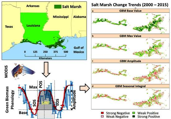
:In this study, we examined the phenology of the salt marsh ecosystem across coastal Louisiana (LA) for a 16-year time period (2000–2015) using NASA’s Moderate Resolution Imaging Spectroradiometer’s (MODIS) eight-day average surface reflectance images (500 m). We compared the performances of least squares fitted asymmetric Gaussian (AG) and double logistic (DL) smoothing functions in terms of increasing the signal-to-noise ratio from the raw phenology derived from the time-series composites. We performed derivative analysis to determine the appropriate start of season (SOS) and end of season (EOS) thresholds. After that, we extracted the seasonality parameters in TIMESAT, and studied the effect of environmental disturbances/anomalies on the seasonality parameters. Finally, we performed trend analysis using the derived seasonality parameters such as base green biomass (GBM) value, maximum GBM value, seasonal amplitude, and small seasonal integral. Based on root mean square error (RMSE) values and residual plots, we selected the best thresholds for SOS (5% of amplitude) and EOS (20% of amplitude), along with the best smoothing function. The selected SOS and EOS thresholds were able to capture the environmental disturbances that have affected the salt marsh ecosystem during the 16-year time period. Our trend analysis results indicate positive trends in the base GBM values in the salt marshes of LA. However, we did not notice as much of a positive trend in the maximum GBM levels. Hence, we observed mostly negative changes in the GBM amplitude and small seasonal integral values. These negative changes indicated the overall progressive decline in the rates of photosynthesis and biomass allocation in the LA salt marsh ecosystem, which is most likely due to elevated atmospheric carbon dioxide levels and sea level rise. The results illustrate both the relative efficiency of MODIS-based biophysical models for analyzing salt marsh phenology, and performances of the smoothing techniques in terms of improving the signal-to-noise ratio of the MODIS-derived phenology.

1. Introduction
The global average atmospheric carbon dioxide (CO2) concentration has risen significantly since the pre-industrial revolution level of 280 ppm [1]. Such increasing levels of CO2 will have wide-ranging consequences on an ecosystem’s structure, function, and services; many natural systems have already started showing signs of being affected [2,3,4]. The conservation and restoration of natural ecosystems, especially those with high carbon sequestration capacity, is crucial in order to offset the rising levels of atmospheric carbon [5]. Salt marshes are well-recognized carbon sinks, and the conservation of such a natural ecosystem is critical in order to maintain carbon balance in the environment [6,7]. However, the response of salt marshes to global fluctuations of atmospheric CO2 may differ from the responses of terrestrial or aquatic ecosystems [8]. Studies have demonstrated the differential response of salt marsh plant species to increasing levels of CO2, with C3 plants (e.g., Phragmites) being more productive than C4 plants (e.g., Spartina), which is an effect that has also been found to be enhanced by sea-level rise [9,10]. This reduced productivity of C4 plants puts them at an adaptive disadvantage, where they might be out-competed by C3 species [11], causing massive shifts in biogeochemistry and ecosystem functioning. The continuous monitoring of the phenology of salt marsh ecosystems for the detection and analysis of any such trends is of utmost priority for the successful implementation of conservation and restoration measures, both at site-specific and landscape levels [12].
One way to study and understand the productive health of any vegetation ecosystem is through analyzing long-term spatiotemporal trends in phenology in relation to their environment [10]. Phenological measurements such as the timing of budburst and flowering are now widely used to detect and study the effect of climate variability on vegetation health, both at the site-specific anc broader landscape scale [13,14,15]. Further, phenology has been shown to be an effective indicator of forest and crop management practices [16,17], urban heat islands [18,19], the El Nino Southern Oscillation [20,21,22], and even the impact of allergies on human health [23]. Moreover, the accurate monitoring of vegetation phenology is crucial for the development of global surface energy and water flux models [24], and the global carbon cycle [25,26]. Therefore, phenological properties or seasonality parameters, such as the timing of the start and end of the season, the rate of green-up and brown-down, amplitude, and maximum growth level have become emerging indicators of global environmental changes [27,28].
Satellite-derived biophysical properties have been frequently utilized to understand vegetation phenology such as the onset of leaf greenness in the spring and leaf coloring in autumn [29,30]. Remote sensing-based phenology began with the Advanced Very High Resolution Radiometer (AVHRR) [31], and has been significantly improved with the Moderate Resolution Imaging Spectroradiometer (MODIS) onboard Terra and Aqua satellites [32]. Both AVHRR and MODIS are currently operational, but MODIS provides images with improved spatial resolution (250 m to 1 km versus 1 km), spectral resolution (36 spectral bands versus six), and geolocation accuracy [33]. Studies have utilized MODIS images for monitoring ecosystem phenology at both site-specific and landscape scales [34,35,36,37,38].
Developing algorithms to automatically retrieve land surface phenology metrics from satellite data has been a popular research topic [39,40,41]. However, the nature of satellite data makes it difficult to directly extract phenological metrics [38,42]. Satellite derived time-series data inevitably contain disturbances caused by cloud presence [43], atmospheric variability [44], and aerosol scattering [45], which degrade the data quality and hinder analysis. Therefore, satellite-derived time-series data are commonly quality-screened and/or smoothed to minimize noise and compensate for the absence of data before phenological metrics can be estimated [46]. Several methods based on the interpolation of time-series data have been proposed to remove such noise and reconstruct high-quality time-series products [47,48,49,50,51,52]. The MATLAB-based program TIMESAT [53] allows the user to test different smoothing techniques, along with various statistical filters, for increasing the signal-to-noise ratio and generating noise-free phenology that can be further utilized for generating seasonality parameters [48,54]. After smoothing the raw phenology, most of the start and end of the season are defined using different methods, such as derivative analysis of the smoothed time series, matching phenology dates derived from in situ observations such as PhenoCam, or using known start of season/end of season (SOS/EOS) thresholds on the smoothed time series (particularly for smoothed Normalized Difference Vegetation Index (NDVI) phenology) [32,55].
Phenology has been studied in detail in a variety of different terrestrial environments, such as tropical rainforests, deciduous habitats, and grasslands; it has also been studied in aquatic ecosystems, such as that of phytoplankton [56,57,58,59]. However, very few studies have emphasized the need to analyze the long-term phenology of salt marsh habitats [12,60,61,62]. In this paper, we derived the long-term trends in the phenology and seasonality parameters of the salt marshes in Louisiana (LA) using existing MODIS-derived biophysical parameters, and analyzed the broader implications of the observed trends. We first describe and test methods for deriving noise-free phenology and seasonality parameters for salt marshes in LA. After that, we validate our methods by analyzing the annual variations. Finally, we evaluate the long-term change trends in the seasonality parameters using statistical trend analysis techniques.
2. Materials and Methods
2.1. Study Area
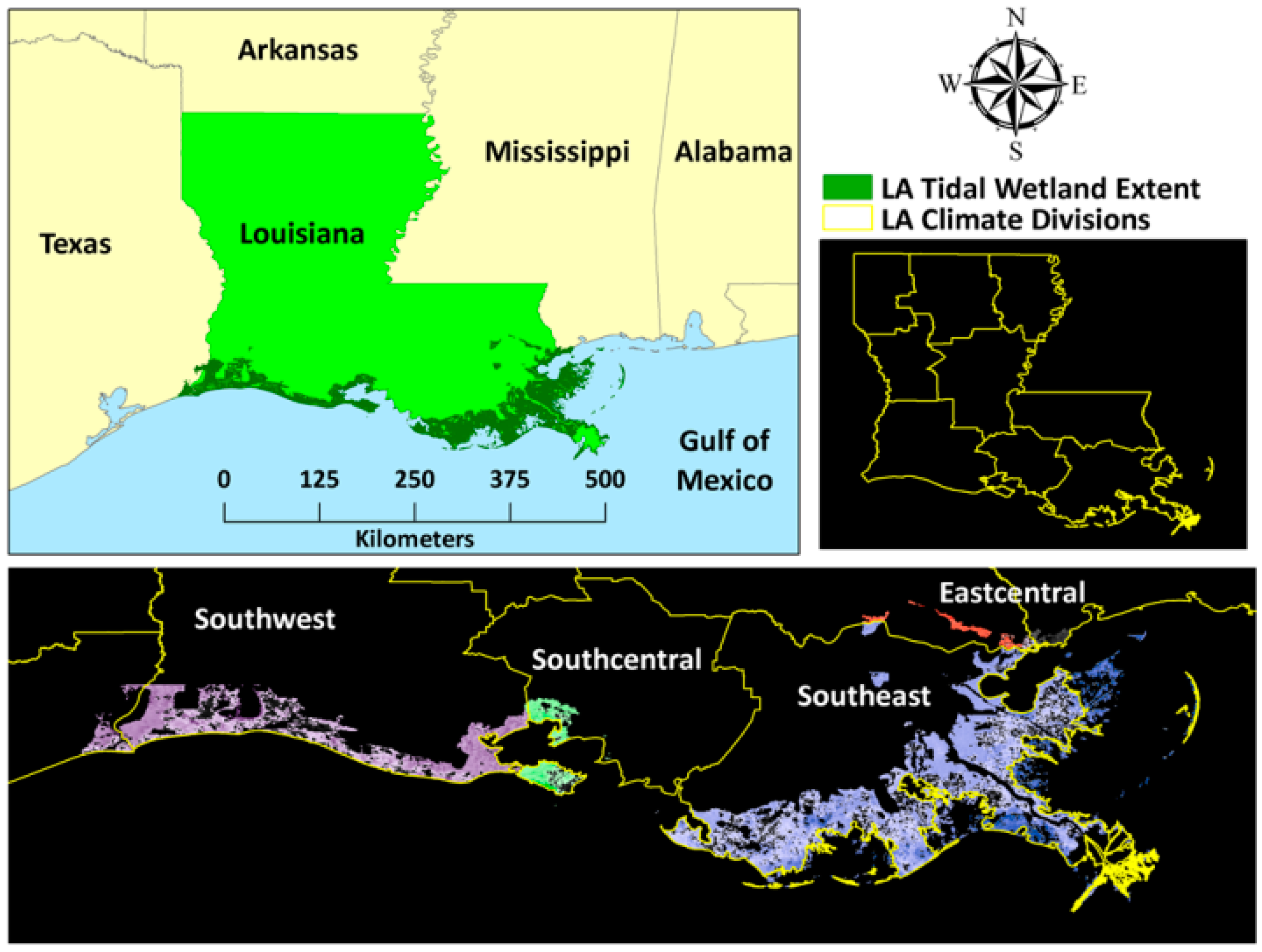
LA has the largest salt marsh ecosystem (>6500 km2) in the United States (US) [63] (Figure 1). The ecosystem is mostly dominated by smooth cordgrass (Spartina alterniflora), and salt meadow cordgrass (Spartina patens). Apart from that, patchy distributions of American Glasswort (Salicornia virginica), saltwort (Batis maritima), and seashore saltgrass (Distichlis spicata) are also encountered. The distribution of black needle rush (Juncus roemarianus) is limited along the brackish regions. The high salinity and anoxic soil do not allow the growth or survival of non-specialized plant species; hence, floral diversity is remarkably low [64]. The climate of the region is tropical to sub-tropical; it is characterized by hot and humid summers, with occasional tropical storms and moderately cold winters. The salt marshes stretch across four state climatic divisions: southwest, south-central, southeast, and east-central [65]. The majority of the salt marsh ecosystem falls within the southeast (~4000 km2) and the southwest (~2000 km2) climatic zones. The average annual temperature in this region varies between 15–25°C, while annual precipitation ranges from 80 cm to 100 cm [66]. Since 2000, the salt marsh ecosystem in LA has experienced the landfall of major hurricanes, such as Lili in 2002 (Category 1), Katrina and Rita in 2005 (Category 4 and 3, respectively), Gustav in 2008 (Category 2), and Isaac in 2012 (Category 1) [67]. The marsh ecosystem in LA is also home to more than 160,000 oil and gas wells [68] that account for almost 18% of the oil and 24% of the natural gas production in the US, and are valued at $6.3 billion and $10.3 billion, respectively [69]. Hence, these ecosystems have been subjected to intense dredging and channelization for transportation as well as significant groundwater removal, which has led to soil and marsh erosion and localized subsidence. Further, the sediment flow from the Mississippi River, which typically provides nutrients and substrate for salt marshes, has been extensively trapped and diverted through the excessive construction of levees across the LA coast. Therefore, it is increasingly difficult for the salt marshes to sustain themselves and fight against sea level rise. Disturbed salt marsh ecosystems in the region have been invaded by common reed (Phragmites australis) at certain places [69].
Over the past decade, there has been an increasing number of reports of salt marsh “dieback” in the US. In 2000 and 2007, LA experienced a sudden and acute dieback event (termed “brown marsh”) that affected over 100,000 ha of Spartina alterniflora-dominated salt marsh throughout the Mississippi River deltaic plain [70,71]. In addition, although the long-term impact is still unknown, the Deepwater Horizon oil spill in 2010 had a severe short-term impact on the health of several fringe and interior salt marsh patches of LA, which was characterized by the loss of chlorophyll and biomass, and subsequently a reduction in photosynthetic capacity [60,72,73].
2.2. Time-Series Composites
The MODIS Land Science Team provides several data products derived from MODIS observations to the public, including the eight-day composite Land Surface Reflectance (MOD09A1). The MOD09A1 datasets include seven spectral bands at a spatial resolution of 500 m corrected for the effects of atmospheric gases, aerosols, and thin cirrus clouds [74]. We generated time-series composites for green biomass (GBM) for the salt marshes of LA for a 16-year period (2000–2015) using MODIS eight-day surface reflectance data (500 m). We generated subsets of LA salt marshes using the most recent vector boundaries obtained from the National Wetlands Inventory (NWI) database [63]. We generated GBM composites using the relationship between GBM and the Visible Atmospheric Resistant Index (VARI) [75] described in Ghosh et al. [12], as follows:
The GBM biophysical model was developed using MODIS surface reflectance and in situ estimates of GBM from 200 study plots across the northern Gulf of Mexico. The model produced a R2 of 0.93 and an inherent percent normalized root mean square error (RMSE) of 17.34% in GBM estimation. Ghosh et al. [12] demonstrated the superior performance of VARI for mapping salt marsh GBM using the MODIS 500 m images compared with the near infrared (NIR) based indices such as NDVI; although studies have utilized NIR-based indices to study salt marsh phenology with finer resolution sensors [12,62,76]. The poor performance of the traditional NIR-based indices was attributed to the severe interference of background moisture and tidal signals to NIR wavelengths, whereas the sensitivity of visible bands was argued to be less susceptible to background water signals. While generating GBM composites, we utilized MODIS quality assurance bands to retain only the best quality pixels in the time-series composites [12,74]. This enabled us to assign equal weight to all of the salt marsh pixels for the extraction of phenology, rather than assigning weights based on quality pixels in TIMESAT. However, tidal correction was not performed, as it is not possible to determine the level of the contribution of daily MODIS images to the eight-day surface reflectance imagery, which would otherwise had helped correct for tidal signals using daily tidal fluctuation data [12].
Since the MODIS surface reflectance products have a temporal resolution of eight days, 46 GBM composites were generated per year for the LA salt marshes; thus, for the 16-year study period, 736 composites were generated in total. We analyzed the salt marshes of the southeast and southwest climatic zones separately in order to avoid any discrepancy due to climate variability. We created subsets of salt marsh GBM composites for individual climatic zones, using the LA climate zone boundaries obtained from the National Climatic Data Centre (NCDC) archives [65]. Once subsets were generated for the salt marshes for individual climatic zones, we converted the raw GBM composites to 16-bit signed generic binary format for running TIMESAT [53]. We also compiled temperature, precipitation, and Palmer Drought Severity Index (PDSI) [77] data for the individual climatic zones from the NCDC archives, to investigate any significant temperature, precipitation, and PDSI anomalies during the 16–year period that might potentially contribute to salt marsh phenological trends.
2.3. TIMESAT
Although the pixels for the time-series analysis were carefully screened using the MODIS quality assurance data, the raw time-series data, as derived from the GBM composites, still showed the presence of residual noise, which was possibly generated from short-term localized environmental disturbances, or tides. However, since the GBM composites were generated using a visible band index (VARI), the tidal effect can be assumed to be minimal. We used the MATLAB-based program TIMESAT to generate a pixel-wise, noise-free time series of GBM. A number of methods have been developed to reduce noise prior to the time series, such as Fourier Series [78,79], Best Index Slope Extraction (BISE) [47], logistic curve [80], and Savitzky-Golay filtering [48]. TIMESAT provides options to fit a smooth continuous curve to raw time-series data using asymmetric Gaussian (AG), double logistic (DL), and/or Savitzky-Golay (SG) filters. In these methods, local model functions are fitted to data in intervals around maxima and minima in the time series [48,54]. For the AG smoothing function, the basis function becomes:
Here, x1 defines the position of the maximum or minimum with respect to the independent time variable t; x2 and x3 determine the width and kurtosis of the right half of the function; and x4 and x5 determine the same for the left half of the function.
The basis function for the DL smoothing function is as follows:
where x1 and x3 define the position of the left and right inflection point, respectively, while x2 and x4 give the rate of change at x1 and x3, respectively. Also, for this function, the parameters are restricted in range to ensure a smooth shape [81].
The AG and the DL filters have been found to produce similar results, with the AG filter being less sensitive to incomplete baseline time-series data [82]. We tested both filters for generating a noise-free time series, and then extracting seasonality parameters. The SG filter was not considered to be ideal for deriving a smooth time series, as it was too susceptible to localized noise in the raw phenology generated from the time-series images, and hence might provide erroneous estimates of seasonality parameters [83]. We used the Seasonal-Trend Decomposition by LOESS (STL) method to remove spikes and outliers in the time series. The STL method removes outliers by assigning weights to the values in the time series based on STL decomposition. This method does not depend on ancillary data, and is global in nature [84]. Further, we also eliminated any negative or zero values observed in the raw phenology from our analysis. We specified an adaptive upper envelope assuming any noise to be negatively biased [48,54]. We specified an adaptation strength of two, as a stronger adaptation strength was likely to put too much emphasis on single high-data values, leading to erroneous estimates of seasonality parameters [48,54].
2.4. Determination of Start and End of Season Determination Using TIMESAT and Derivative Analysis
TIMESAT allows the user to specify SOS and EOS dates as a user-defined fraction of the seasonal amplitude. We derived SOS and EOS using different thresholds (fractions of seasonal amplitude), such as 5%, 10%, 15%, and 20%. We did not test thresholds below five percent, as it might be influenced by the noise from the non-growing season [55]. Phenology studies using TIMESAT have mostly preferred to use thresholds above 10% (usually 20%; sometimes 50%) for deriving SOS and EOS dates using a NIR wavelength-based vegetation index time series. Most of these thresholds are usually determined based on expert opinions or in-field observations of the SOS and EOS [85,86,87]. However, the phenology of the salt marsh ecosystem has neither been studied in detail, nor did we have any in–field monitoring stations observing real-time SOS and EOS dates that could have been the basis for choosing or validating appropriate thresholds of SOS and EOS for TIMESAT. Temperature variations at the start and end of the growing season may be used to determine the SOS and EOS; however, plant phenology and seasonality parameters are not only influenced by temperature, but also by other environmental variables or local environmental disturbances and dynamics. Further, the NDVI time series or thresholds could not be utilized for deriving SOS and EOS, as NDVI or any NIR-based indices are prone to insensitivity in salt marsh settings [12]. GBM was derived from MODIS 500 m eight-day surface reflectance composites for LA marshes using the VARI [75], which had been shown to be more sensitive than NIR-based indices, especially for salt marshes with perpetually saturated soil [12]. Therefore, we tested the performances of different thresholds by matching the SOS and EOS dates derived using derivative analysis against dates derived using different thresholds in TIMESAT, as described in the following paragraph.
Unfortunately, there is no specific universal threshold that can be applied to estimate SOS and EOS dates; and calibration is necessary before the selection of any specific threshold. We investigated the derivatives of smoothed GBM time-series data, which were derived using both AG and DL methods from ~400 random pixels. We estimated the third-order derivative from the smoothed time series, and derived local maxima and minima [83]. The third-order derivative has been demonstrated as a better indicator for identifying SOS and EOS than the second order, as the latter represents the timing when the majority of vegetation within a pixel is turning green, rather than the timing when the change of green-up rate or brown-down rate is the greatest [83]. For the SOS and EOS, we matched the local maxima and local minima, respectively, with the SOS and EOS dates derived using different thresholds in TIMESAT. We did this using a smoothed time series derived by employing both AG and DL smoothing functions in TIMESAT. We did not analyze derivatives for peak of season (POS) date estimations, as POS is a function of the maximum value encountered in the middle of the growing season, and it does not depend on the thresholds chosen for SOS and EOS. Once we matched SOS and EOS dates derived from derivative analysis against TIMESAT thresholds, we estimated the error between the observations using root mean square error (RMSE), and also analyzed residual plots for any specific trends. We selected the TIMESAT SOS and EOS thresholds that illustrated the greatest agreement with the dates derived from derivative analysis. After that, we derived the SOS and EOS for the entire salt marsh landscape using the best SOS and EOS thresholds and the best smoothing technique in TIMESAT, for further analysis and validation.
2.5. Analysis of SOS and EOS Fluctuations for the Validation of Thresholds
We did not have any in situ observations of SOS and EOS to validate the dates derived using the best thresholds in TIMESAT. Therefore, we further attempted to validate our thresholds for SOS and EOS through analyzing the interannual variations of SOS and EOS, and investigating whether the major observed deviations from the normal trends in SOS and EOS can be explained by occurrences of environmental disturbances/anomalies (such as temperature anomalies, hurricanes, drought, or other natural/anthropogenic disasters) that might have influenced those deviations. Here, we derive the SOS and EOS for the salt marshes of southeast and southwest LA using the best thresholds in TIMESAT. We analyzed southeast and southwest LA separately, as the nature and effect of environmental disturbances on SOS and EOS may vary across climatic zones. Further, the southeast and the southwest climatic zones of LA comprise entirely salt marsh habitats; hence, the effect(s) of any localized environmental disturbance(s) within the climatic zones will be manifested entirely in the salt marsh phenology. The analysis attempts to provide further justification of the SOS and EOS thresholds chosen for deriving the seasonality parameters of the LA salt marshes.
2.6. Seasonality Analysis and Simple Linear Trend Analysis
TIMESAT allows its user to derive various seasonality parameters using time-series data (Table 1). We extracted seasonality parameters, such as base value, max value, amplitude, and small seasonal integral, which are major indicators of seasonal photosynthesis and biomass production and accumulation, for all of the salt marsh pixels covering coastal LA for 16-year period. Once extracted, they were analyzed for seasonal fluctuations. Possible reasons behind the seasonal fluctuations were investigated through the careful study of environmental events such as temperature and precipitation anomalies, the landfall of tropical storms, man-made hazards, or other climatic hazards such as drought causing possible localized dieback, which might trigger an early end to a growing season, or a subsequent late/early start of a growing season. After that, we examined the overall trend in these seasonality parameters using simple linear regression. We examined the slope of the fitted trendline to determine any overall positive and negative trends over the 16-year time period based on the positive or negative value of the slope magnitude.
2.7. Trend Analysis
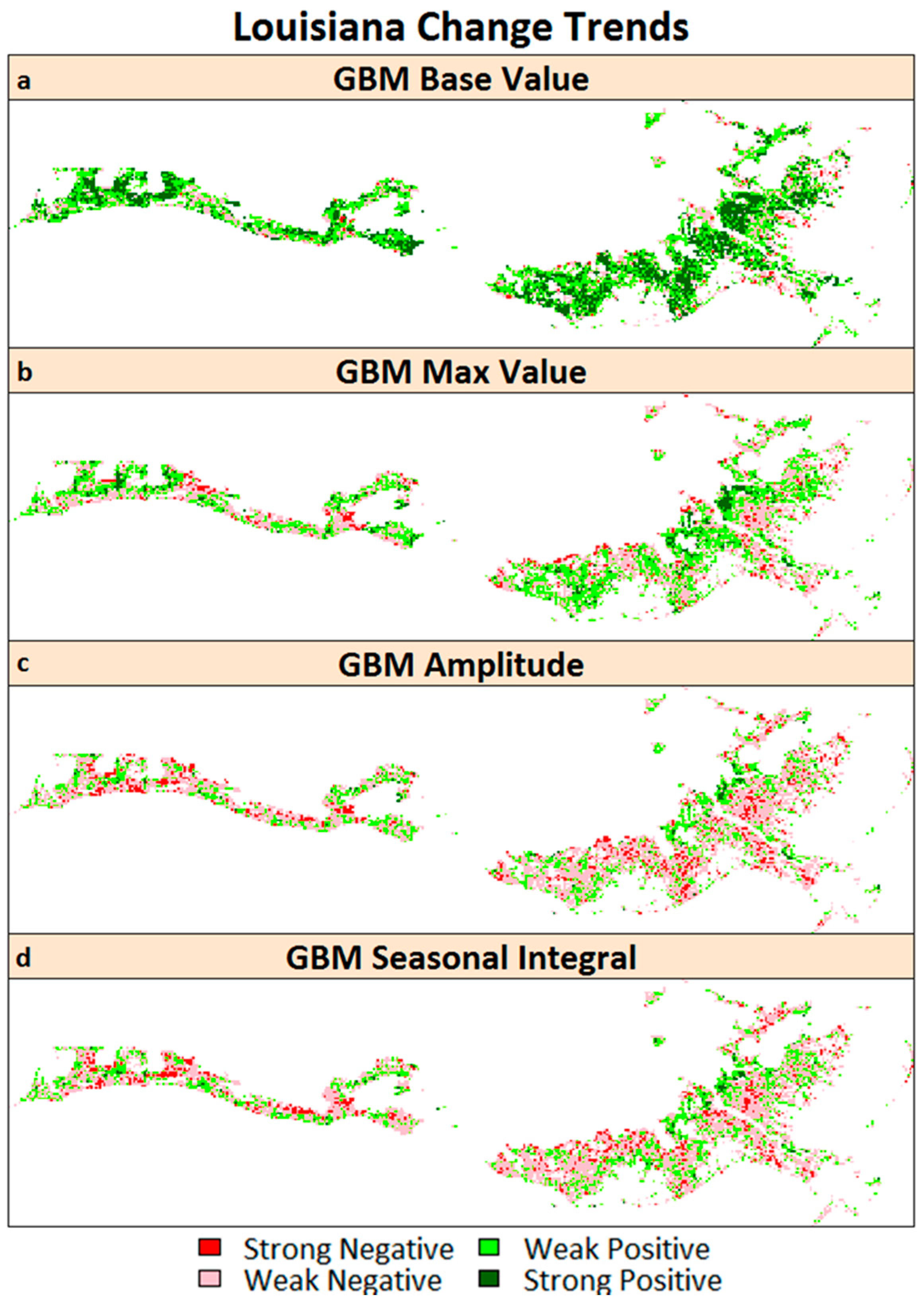
In order to highlight the spatial distribution of the marsh pixels showing improvement (positive change) and stress/degradation (negative change), we employed the Mann-Kendall (MK) trend test [88] to determine the phenological changes of the salt marshes of southeast and southwest LA between 2000–2015, using R [89]. We calculated the MK trend test separately for every pixel for base value, amplitude, max value, and small seasonal integral composites for the southeast and southwest LA salt marshes. These parameters are crucial indicators of seasonal productivity. We classified changes based on the z-score distribution at a 95% confidence interval. A positive or negative value of z represented an upward or downward trend, respectively. Changes beyond the lower critical limit (z < −1.96) were classified as a strong negative change, while those beyond the higher critical limit (z > 1.96) were classified as a strong positive change. Changes within the 95% confidence interval were classified as weak (negative or positive depending on negative or positive values of z).
3. Results
3.1. SOS and EOS Determination
3.1.1. Derivative Analysis versus TIMESAT
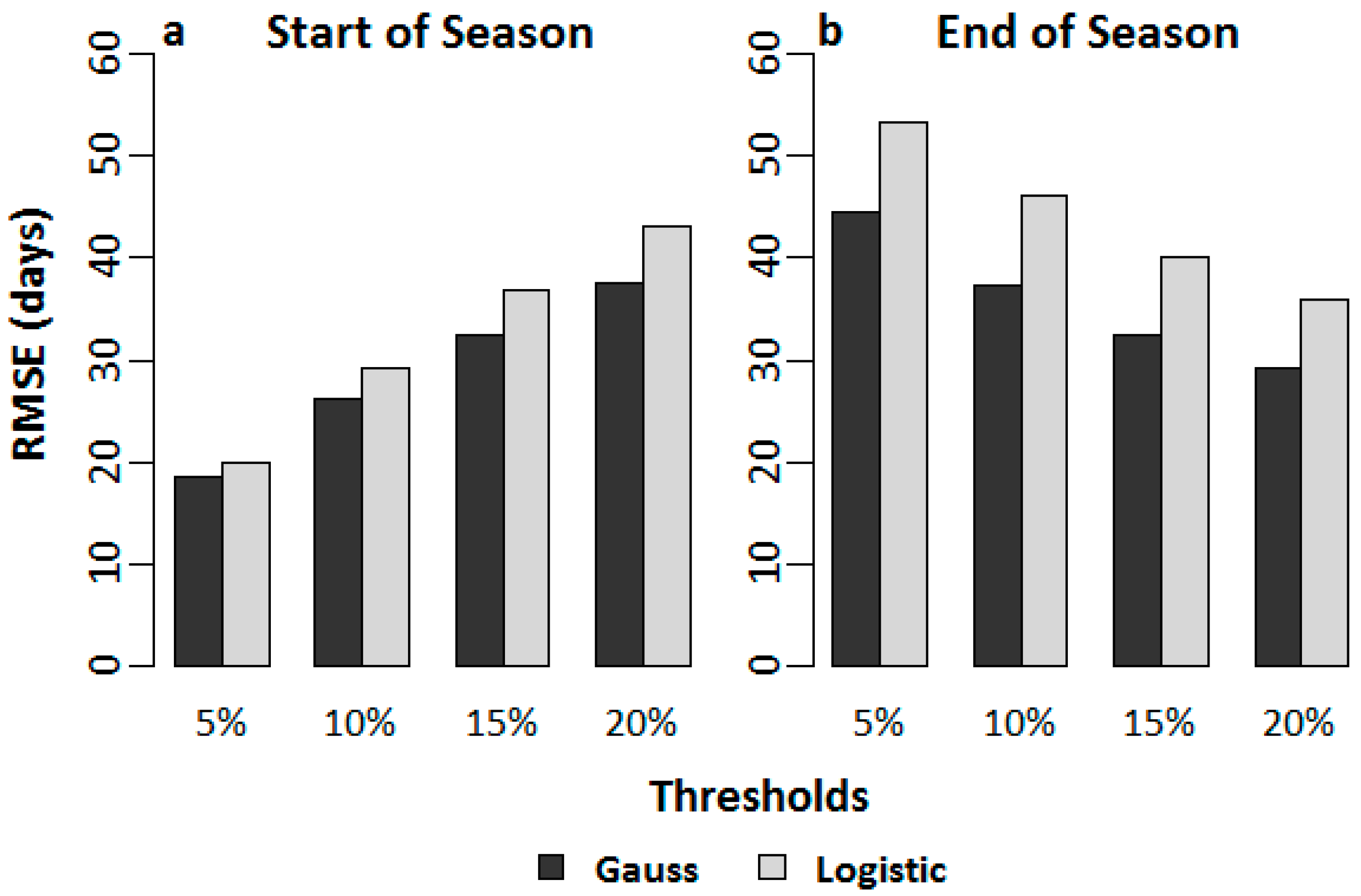
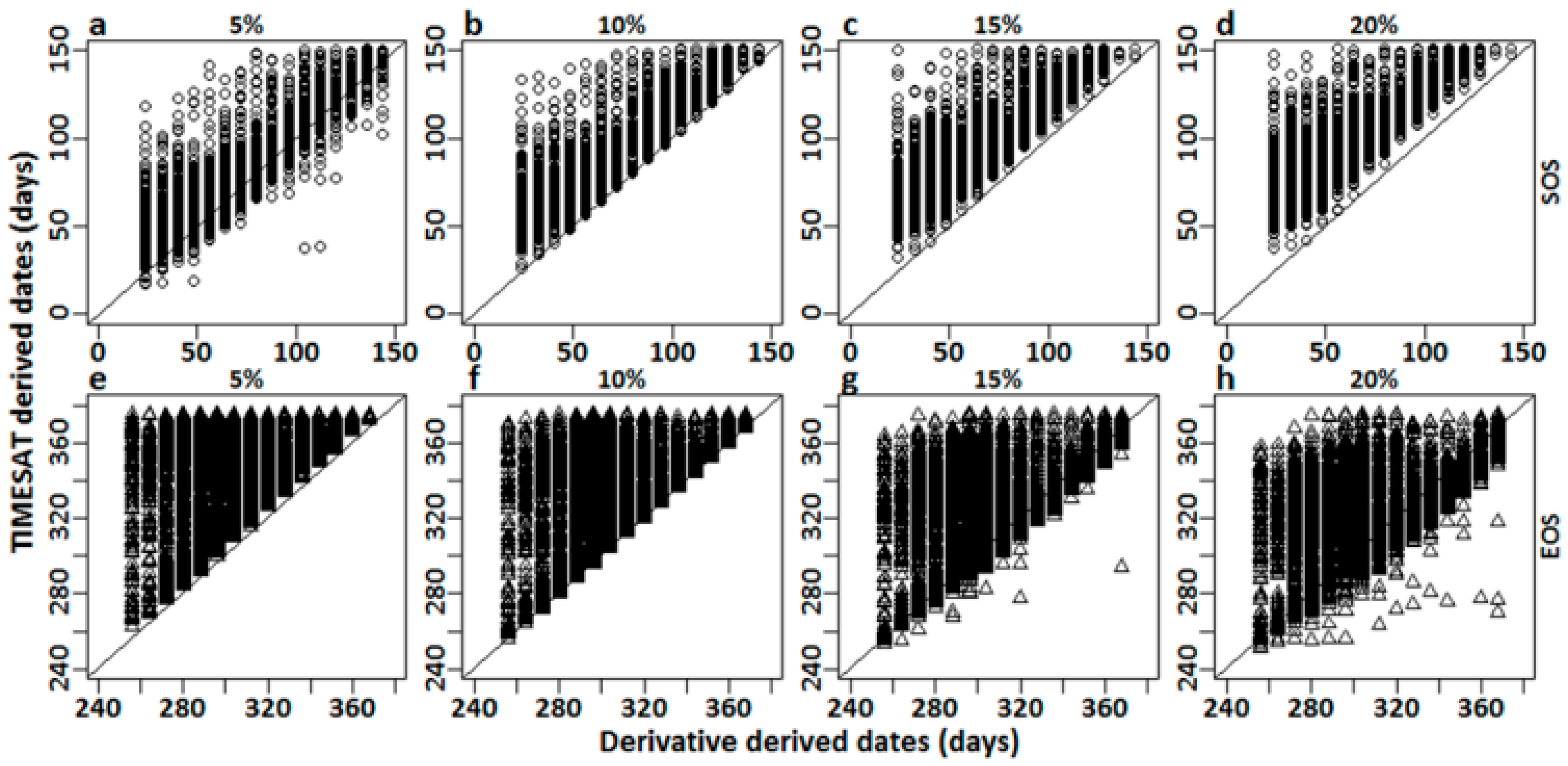
Results from the derivative analysis showed similar trends for both the AG and DL methods of smoothing. For the SOS (Figure 2a), the 5% threshold seemed to agree the most with the derivative analysis for both the AG and DL smoothing functions with the lowest RMSE. Higher thresholds showed greater RMSEs. The SOS dates derived using the AG method agreed with the derivative-derived dates marginally better than the DL method; the AG method showing an error of ~25 days for the 5% threshold and ~28 days for the DL method. The residual plots for the SOS showed no specific trends for the 5% threshold (Figure 3a). Higher thresholds predicted late SOS dates when compared with the derivative derived dates (Figure 3b–d). For the EOS, the 20% threshold showed the highest agreement with the derivative–derived EOS dates (Figure 2b), with errors progressively increasing with lower thresholds (Figure 3e–h). The residual plots also demonstrated late EOS predictions with progressive decreasing thresholds compared with the derivative-derived EOS dates (Figure 3b). The AG method again agreed more closely with the derivative-derived dates than the DL method in the estimation of EOS. For the best threshold (20%), the AG method showed an error of ~29 days, while the same for the DL method was ~40 days. However, as mentioned before, we did not have any in situ observations of the SOS and EOS to validate the dates derived using asymmetric thresholds in TIMESAT. Therefore, the only way to validate our thresholds for the SOS and EOS was through analyzing the interannual variations of the SOS and EOS, and investigating whether the major deviations from the normal trends in the SOS and EOS observed can be explained by occurrences of environmental disturbances/anomalies that might have influenced those deviations.
3.1.2. SOS and EOS Validation through Analysis of Fluctuations
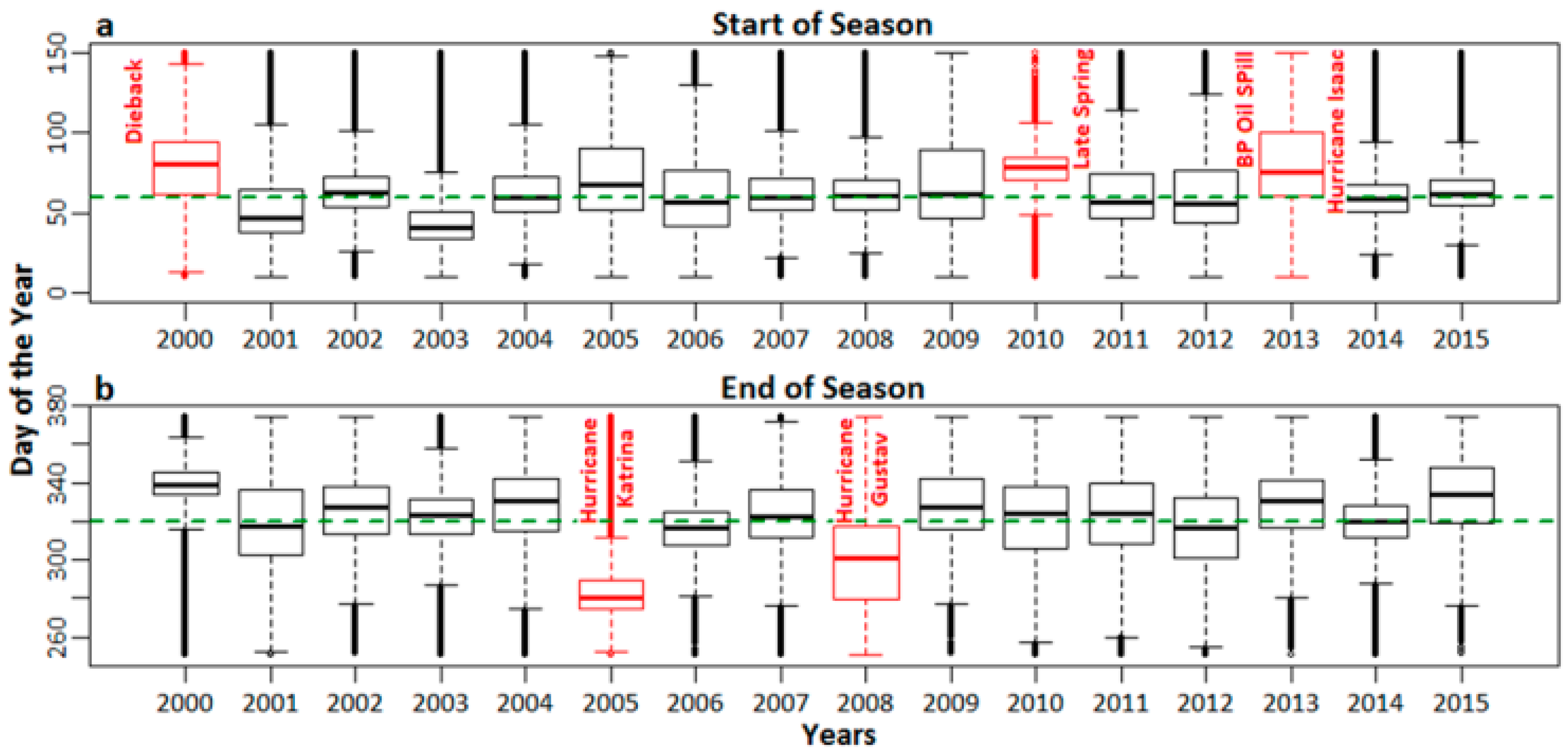
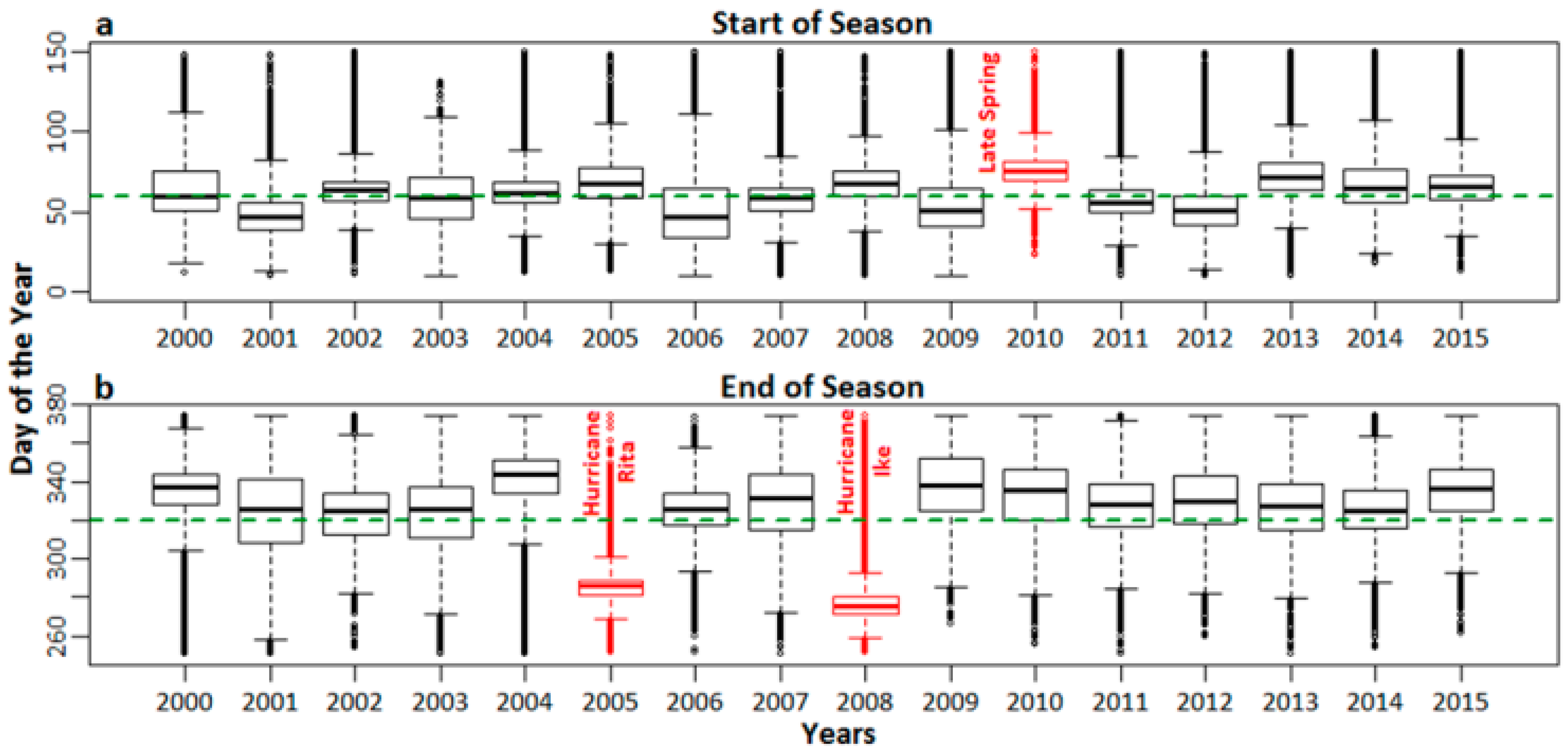
The median SOS date for the salt marshes of southeast and southwest Louisiana as derived from TIMESAT was observed at ~60 Julian days (Figure 4a and Figure 5a). However, in the years 2000, 2010, and 2013, the salt marshes of southeast LA showed a late SOS. A late SOS was also observed in southwest LA in 2010. The median EOS for the LA salt marshes was observed at ~322 Julian days. The salt marshes of both southeast and southwest LA experienced an early end to the growing season in the years 2005 and 2008.
3.2. Seasonality Analysis and Simple Linear Trends
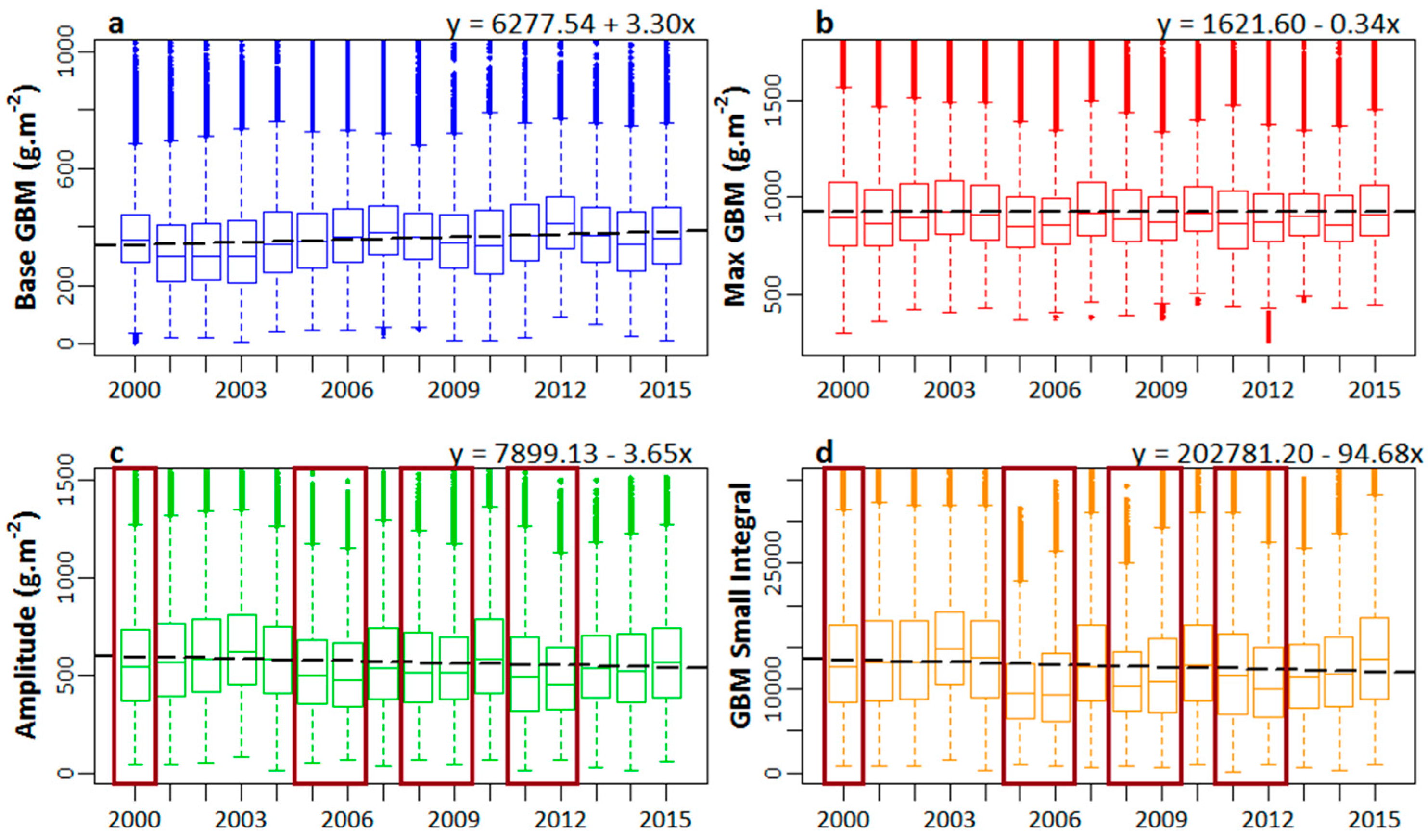
Simple linear trends in GBM base values, GBM max values, seasonal GBM amplitude, and small GBM integral are shown in Figure 6. Overall, during the 16-year study period, the GBM base values showed positive trends (Figure 6a) and GBM max values remained stable, while the rest of the seasonality parameters showed negative trends (Figure 6b–d). We also observed a periodic decline in the levels of GBM amplitude and GBM small integral in the years 2000, 2005–2006, 2008, and 2011–2012. However, we noticed subsequent improvements in the levels of these seasonality parameters after the short-term decline as well, when environmental conditions improved.
3.3. Mann-Kendall Trend Analysis
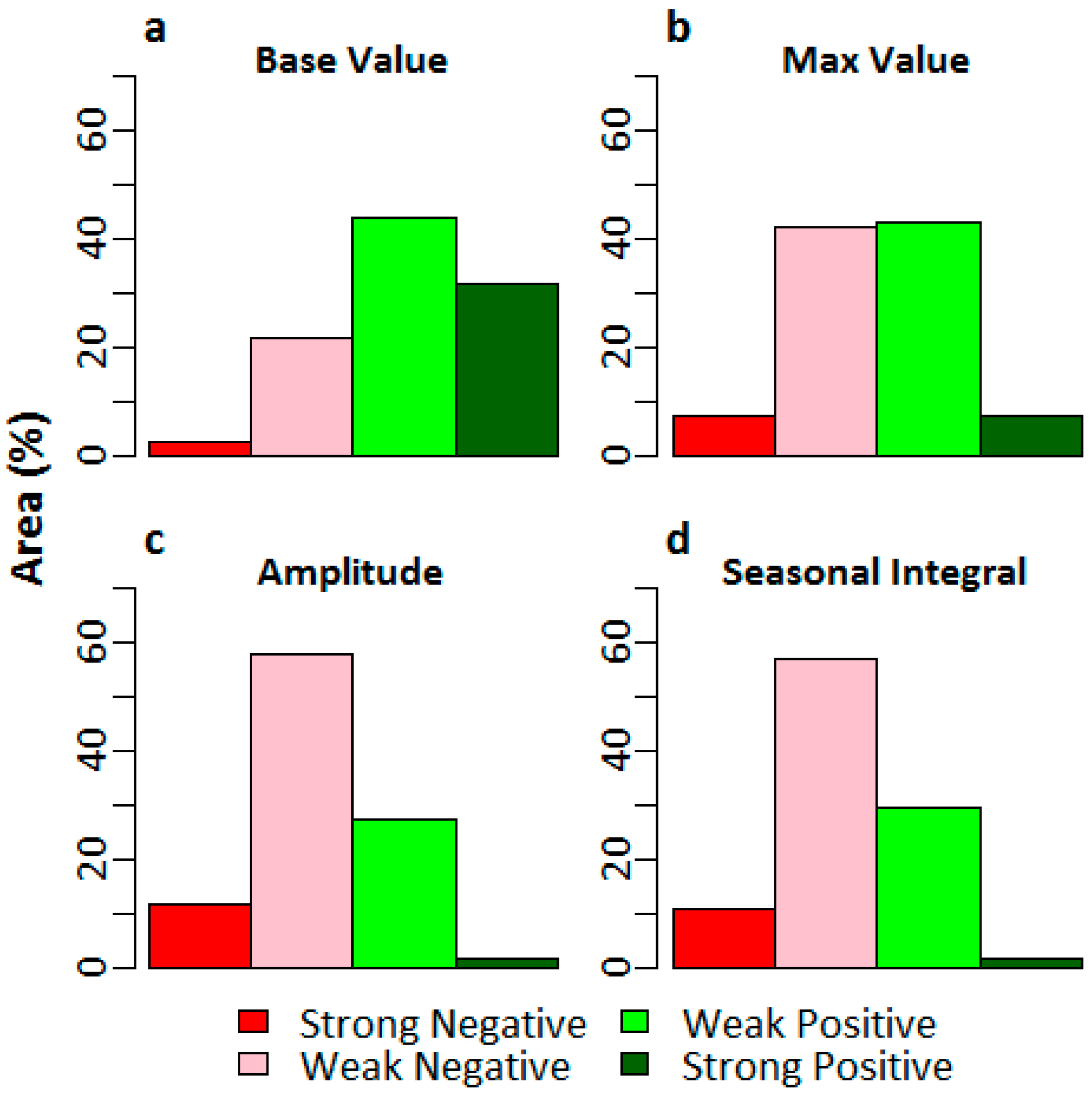
Trend classes for changes in the base values, max values, seasonal amplitudes, and small seasonal integrals (refer to Table 1 for description and phenological significance) for the southeast LA salt marshes are shown in Figure 7. We observed positive changes in the GBM base values in almost 75.5% of the salt marsh area in southeast LA, with strong positive changes observed in 31.6% of the area. However, the max values did not show as much positive change; we observed strong positive changes in only 7.2% of the total salt marsh area. On the other hand, we observed mostly negative changes in the seasonal amplitude and small seasonal integral, two parameters that are indicators of net seasonal photosynthesis rates and biomass productions. Most (70.3%) of the salt marsh ecosystem showed negative changes in seasonal amplitude (with 12.1% of the area showing a strong negative change), while 67.9% showed negative changes in the small seasonal integral (with 10.9% of the area showing a strong negative change). Overall, the areas with positive changes in base values and negative changes in the seasonal amplitude and small seasonal integral matched well (Figure 8).
4. Discussion
4.1. SOS and EOS Determination
4.1.1. Derivative Analysis vs. TIMESAT
As evident from matching the SOS and EOS dates from derivative analysis with those from TIMESAT, both the AG and DL smoothing filters performed similarly. This was not unexpected, since previous studies have shown similar behaviors for these two methods [82]. Further, the 5% threshold for the SOS agreed the most with the SOS dates that were derived from derivative analysis, while the 20% threshold displayed the highest agreement with the derivative analysis derived EOS dates. Although seasonality parameters are usually derived using symmetric thresholds, asymmetric thresholds may not be uncommon for AG or DL smoothing filters, as both smoothing functions demonstrated skewness.
4.1.2. SOS and EOS Validation through Analysis of Fluctuations
The median SOS date for the salt marshes of southeast and southwest Louisiana as derived from TIMESAT was ~60 Julian days (Figure 4a and Figure 5a), which corresponds with the onset of spring at the end of February and beginning of March. However, in the years 2000, 2010, and 2013, the salt marshes of southeast LA displayed a late SOS. The year 2000 had witnessed an acute recurring dieback event that affected almost 100,000 ha of marshes in LA [71,90]. This dieback might have resulted from extremely dry conditions for two consecutive years (1999 and 2000) [65]. The acute dieback event had most likely delayed the normal SOS date in 2000. The delayed start to the 2010 growing season was most likely due to the late onset of spring owing to colder than normal temperatures at the beginning of the season [65], a phenomenon also observed in the salt marshes of southwest LA.
Finally, the delayed SOS in 2013 might be due to the aftereffects of the Deepwater Horizon oil spill (2010) and Hurricane Isaac (2012). The residual oil and the cleanup efforts had negative effects on the marsh patches in southeast LA, and the restoration efforts may have been affected by the landfall of tropical storm Bonnie in 2010, which brought additional oil into the shoreline marsh. The short-term degradation due to the oil spill, subsequent cleanup, and the efforts and stress induced by tropical storm Bonnie, all delayed the peak growth of the marsh patches in the area in 2011 [60]. In spite of this, the marshes had started to recover from oil spill effects in 2011 [91]. However, the recovery of the marsh patches was further damaged by the landfall of Hurricane Isaac in 2012, during the peak of the growing season. Although Hurricane Isaac was a Category 1 hurricane, the timing of the landfall had an adverse effect, as the salt marshes were unable to achieve full recovery from the stress induced by the oil spill. That could be the reason why we noticed another delayed dormancy onset in 2013. Our observations are consistent with those made by Khanna et al. [92]. Any residual oil effects in 2011 or 2012 might have been localized, as the marshes had started to recover or had already recovered from the effects of the oil spill. Those localized effects were not severe enough to have manifested in the MODIS data. Further, the biomass model has a 17% error, so a minor localized disturbance that produced a localized effect in the biomass level may have been below the error threshold, and thus not have been picked up by the model.
The salt marsh growing season in LA normally ends around mid-November (Figure 4b and Figure 5b), which was observed in both southeast and southwest LA, with the median EOS date being ~322 Julian days. However, the salt marshes in both these regions experienced an early end to the growing season in 2005 and 2008. In southeast LA, Hurricane Katrina made landfall in September as a major Category 3 hurricane that destroyed most of the salt marsh ecosystem [93], which was unable to recover in the same year. A similarly drastic EOS was observed in the year 2008, when Hurricane Gustav made landfall; however, the effects of the landfall were not as severe as Katrina. In southwest LA, landfalls and subsequent damages caused by Hurricane Rita (2005) and Hurricane Ike (2008) were the main reasons for the early EOS in those respective years. These results provide justification to the SOS and EOS thresholds chosen for the derivation of seasonality parameters, as they have been able to capture the environmental events that have affected the SOS and EOS of the salt marsh ecosystem during the 16-year time period.
4.2. Seasonality Analysis and Simple Linear Trends
The positive trend observed in the base GBM values is an indicator of the cumulative storage of carbon over time as aboveground biomass. However, the max GBM values remained almost stable during the 16-year period. Meanwhile, negative changes were observed in seasonal amplitude and seasonal integral, which indicated the long-term stress that had been induced in the salt marsh vegetation, resulting in reduced photosynthesis and aboveground biomass accumulation. We observed severe short-term effects of the periodic dieback events occurring in the salt marsh habits in the years 2000 [94], 2006 [90], and 2011 [95], and the landfalls of major hurricanes in 2005 (Katrina and Rita) [96,97], 2008 (Gustav and Ike) [98], and 2012 (Isaac) [99], which affected the seasonal photosynthetic activity of the salt marsh habitats. These severe short-term effects were evident from the relative lower magnitudes of seasonal amplitude and small integral, as observed for those time periods. However, we also observed the recovery of the marsh habitats from the stress induced by dieback events and hurricane landfalls, when the environmental conditions became normal and conducive for salt marsh vegetation growth.
4.3. Mann-Kendall Trend Analysis
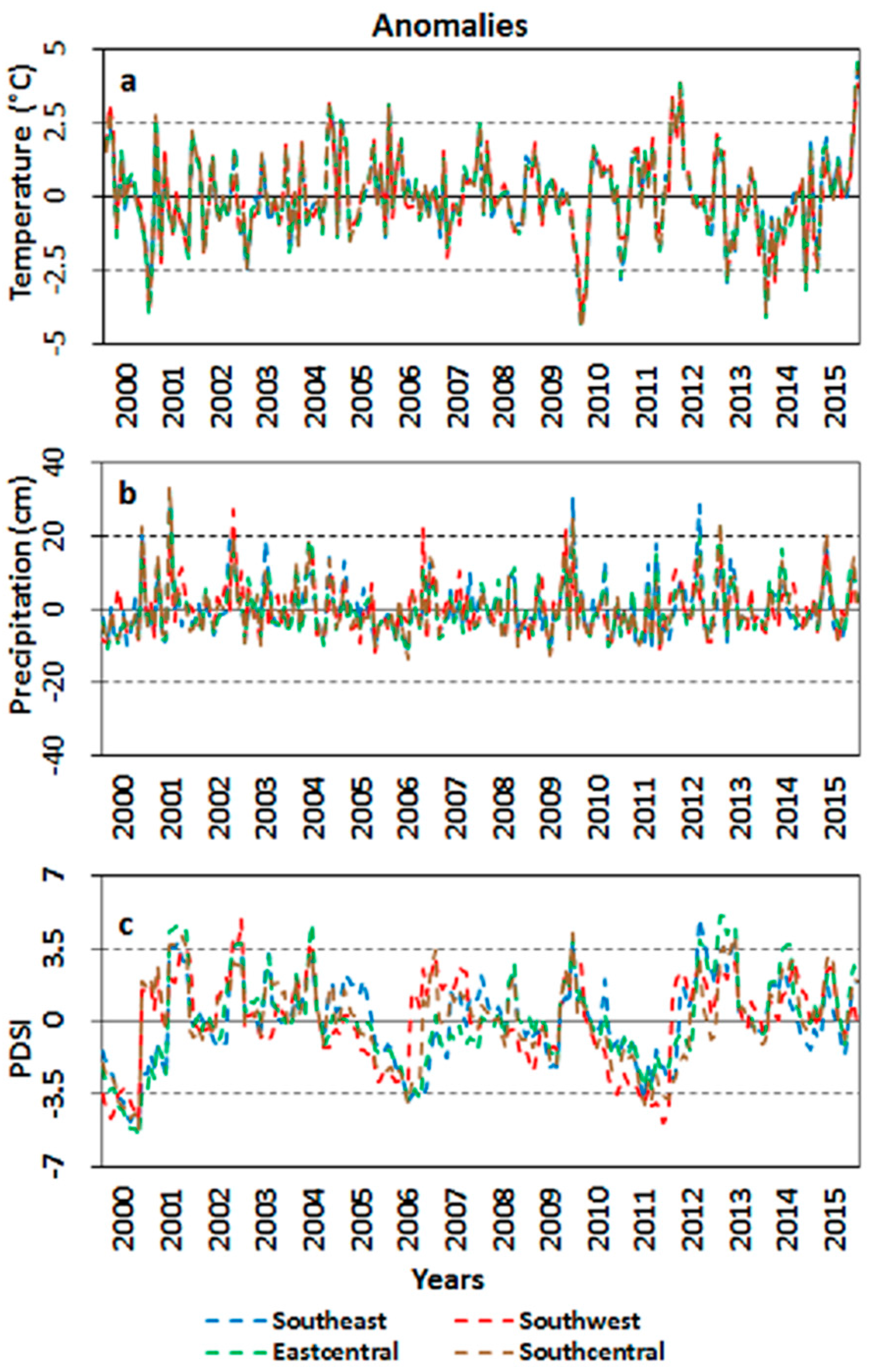
Most of the salt marsh ecosystem showed a progressive increase in the base GBM value, indicating that a considerable amount of carbon had been accumulated over time and stored as aboveground biomass in the salt marsh ecosystem. Interestingly, the maximum GBM value did not show as much progressive increase as the base GBM value, indicating that the maximum biomass as well as maximum photosynthesis rate had reached a level of saturation. Therefore, strong negative changes in seasonal amplitude and small seasonal integral were observed, which indicated a progressive decline in the levels of the net seasonal photosynthesis rate over the 16-year time period. Normally, changes in the levels of photosynthesis are attributed to changes in the levels of temperature and precipitation, as they influence the photoperiod and salinity of the ecosystem [100,101]. However, neither the temperature nor the precipitation anomalies for either southeast or southwest LA showed any particular trend during the 16-year time period (Figure 9). The salt marsh ecosystem of these regions has experienced periodic diebacks; however, since salt marshes are resilient ecosystems, they are capable of recovering from short–term environmental stress if environmental conditions become normal again [73].
Atmospheric CO2 levels rose from 369 ppm to 404 ppm during the period 2000–2015 [1], while sea levels were observed rising at a rate of 9–12 mm·year−1 in coastal LA [102]. Elevated CO2 levels in the atmosphere have been known to induce photosynthetic saturation in C4 plants; the saturation generally initiates at carbon dioxide concentrations beyond 350 ppm [103]. In salt marsh habitats, elevated atmospheric CO2 levels have been observed to reduce both above and belowground biomass allocation in C4 plant species [9,10], as a result of a reduction in stomatal conductance [104], as well as the rate of water usage [9,10,105] ultimately reducing the rate of photosynthesis. White et al. [9] observed a greater reduction in the aboveground biomass allocation of C4 plants than C3 plants in response to elevated CO2 and sea level rise in a salt marsh habitat, even with altered nutrient levels in the environment. The salt marsh ecosystem in Louisiana is mostly dominated by the smooth cordgrass (Spartina alterniflora) and salt meadow cordgrass (Spartina patens), both of which are C4 species. Therefore, in light of the observed rise in CO2 levels and sea level rise, this observed reduction in the level of net photosynthesis and biomass allocation in the salt marshes of LA is not entirely unexpected. Although we haven’t done any field experiments to test this, there have been many studies over the past decade confirming the phenomena using observed datasets.
If the progressive decline in the rates of photosynthesis and biomass allocation continues, the carbon sequestration rate of the LA salt marsh ecosystem might not be able to keep up with the rate of rising atmospheric CO2; rather, with periodic disturbances such as hurricanes, dieback, and anthropogenic disasters, marsh loss will turn the ecosystem to carbon sources [106]. On the other hand, such elevated levels of atmospheric CO2 and sea levels will stimulate photosynthesis, water usage capacity, and more efficient biomass allocation in C3 plants compared with C4 plants [9,10]. This might explain the invasion of Phragmites australis in the coastal salt marsh landscape of LA [107]. Phragmites has a variable photosynthetic pathway that is capable of exhibiting both C3 and C4 photosynthesis [108]. Under elevated levels of CO2, the C3 pathway will probably become dominant in Phragmites, and this would allow the plant to dominate the coastal salt marsh ecosystem, especially if the ecosystem experiences nitrogen enrichment through runoff [109]. If Phragmites displaces Spartina as the dominant species in the coastal marsh landscape, there might be far-reaching ecological consequences such as changes in plant species abundance [110] and trophic interactions [111,112], herbivore population crashes [113], and changes in soil biogeochemistry [114]. In this research, we don’t claim that such a phenomenon is already underway, as it is beyond the scope of this study, but supporting evidence from our analysis suggests that there is a risk of such a cascading effect in future.
5. Conclusions
This study provides a comprehensive analysis of the phenological trends of the salt marsh ecosystem of LA, showcasing the efficiency of the MODIS-based biophysical model derived time-series composites of salt marsh GBM. We used TIMESAT to generate noise-free phenology from the GBM time-series composites after determining the SOS and EOS thresholds using derivative analysis. We justified our selection of the best smoothing algorithm (AG) and SOS/EOS thresholds after matching the SOS and EOS dates derived using derivative analysis and TIMESAT thresholds. We analyzed the seasonality in the SOS and EOS dates over a 16-year time period; the effects of the environmental events influencing the deviations from the normal SOS and EOS have been efficiently captured. Finally, the trend analysis demonstrated a reduction in the rates of seasonal amplitudes and small seasonal integrals, and improvement in the levels of GBM base values, indicating the progressive reduction in the levels of photosynthesis and biomass allocation in the salt marsh ecosystem that might be attributed as a combination of environmental effects such as rising atmospheric CO2 levels and sea level rise.
Further, the trend analysis results have been able to capture areas that are demonstrating significant stress in terms of reduced photosynthetic activity and thus require immediate restoration and conservation efforts. The results of this study can be compared with Gross Primary Productivity (GPP) trends as observed from the MODIS 500-m and 1-km GPP products; however, MODIS GPP products for coastal wetlands are derived using very generic grassland light use efficiency (LUE) estimates from a Biome properties look-up table that do not incorporate tidal effects or other conditions specific to coastal marshes. Therefore, caution should be exercised when drawing conclusions derived from GPP trend matching. Although trend analysis using MODIS-derived images can provide a valuable insight into the phenological dynamics at the landscape level, site-specific trend analysis might require a similar analysis using site-specific records of sea level changes, nitrogen enrichment, and salinity, along with finer resolution images. In addition, with finer resolution images, it will be possible to determine the distribution dynamics of the invasive Phragmites australis in an otherwise Spartina-dominated landscape, and compare the progressive phenological trends of the two species with respect to elevated CO2 levels and sea level rise. Such a future study will provide a clearer picture regarding the possible ecological succession of Spartina by Phragmites.
In addition, due to the coarse nature of the MODIS sensor, the possibility of encountering mixed pixels cannot be ruled out, especially while studying a highly fragmented ecosystem such as a salt marsh. One way to address the issue is to mask out mixed pixels completely from the analysis. However, ignoring or eliminating mixed pixels often poses the problem of eliminating the critical shoreline of salt marsh habitats from the analysis, which are often the most sensitive to environmental changes. Therefore, the selection of the appropriate vegetation index that is less susceptible to signals from water/tides in the shoreline pixels is crucial. This problem of mixed pixels exists even with finer spatial resolution sensors. Further, most fine spatial resolution sensors do not acquire images at such high temporal frequency as MODIS (daily images combined to generate the eight-day surface reflectance product), which is ideal for the analysis of long-term phenological trends. Further, finer spatial resolution images often present the problem of cloud cover that may render images completely unusable for analysis, resulting in frequent data gaps. This problem is particularly evident in the coastal Gulf of Mexico, where cloud presence in images from fine resolution sensors often hinders analysis, especially during the peak growing season. Further, their spatial coverage/swaths are much less than MODIS; hence, combining scenes from multiple days may create biases in the analysis itself. Hence, for analysis at such broader landscape scale, MODIS is clearly a robust sensor.
This is the first time that such a comprehensive analysis of the phenological trends of the LA salt marsh ecosystem has been studied in terms of the seasonality parameters. Using the suggested methods in this study, the monitoring of salt marsh ecosystem in LA, the southeast US, and elsewhere in the world with similar environmental settings will be possible, following the necessary re-parameterization of the GBM model. Through continuous monitoring of the ecosystem, it will be possible to ascertain whether salt marshes will continue to be a major carbon sink in the environment, or changes in the environment will force them to become a net carbon source. As mentioned before, salt marshes are dynamic and critical ecosystems in terms of carbon sequestration. Therefore, continuous monitoring of these critical ecosystems is crucial for effective restoration and management practices and the formulation of global change policies.
Acknowledgments
We would like to thank and acknowledge our project partners at Mississippi State University, University of Nebraska-Lincoln, and University of New Orleans. This research was partially funded by the National Aeronautics and Space Administration (NASA) Gulf of Mexico program (Grant # NNX10AE65G), National Science Foundation (NSF) Division of Environmental Biology (Grant # 1050500), and Gulf of Mexico Research Initiative (GoMRI) (Grant # GRI-0012). Shuvankar Ghosh is grateful to the University of Georgia Graduate School Dean’s Award for Social Science for carrying out this research.
Author Contributions
Shuvankar Ghosh helped with processing of image data, designed the study and wrote the manuscript. Deepak R. Mishra provided invaluable advice during the analysis phase and helped with editing the manuscript.
Conflicts of Interest
The authors declare no conflict of interest.
References
- NOAA Earth System Research Laboratory, Global Monitoring Division. Trends in Atmospheric Carbon Dioxide. Available online: https://www.esrl.noaa.gov/gmd/ccgg/trends/graph (accessed on 25 December 2016).
- Parmesan, C.; Yohe, G. A globally coherent fingerprint of climate change impacts across natural systems. Nature 2003, 421, 37–42. [Google Scholar] [CrossRef] [PubMed]
- Menzel, A.; Sparks, T.H.; Estrella, N.; Koch, E.; Aasa, A.; Ahas, R.; Alm–Kubler, K.; Bissolli, P.; Braslavska, O.; Briede, A.; et al. European phenological response to climate change matches the warming pattern. Glob. Chang. Biol. 2006, 12, 1969–1976. [Google Scholar] [CrossRef]
- Post, E.; Forchhammer, M.C.; Bret-Harte, M.S.; Callaghan, T.V.; Christensen, T.R.; Elberling, B.; Fox, A.D.; Gilg, O.; Hik, D.S.; Høye, T.T.; et al. Ecological dynamics across the Arctic associated with recent climate change. Science 2009, 325, 1355–1358. [Google Scholar] [CrossRef] [PubMed]
- Canadell, J.G.; Raupach, M.R. Managing forests for climate change mitigation. Science 2008, 320, 1456–1457. [Google Scholar] [CrossRef] [PubMed]
- Connor, R.F.; Chmura, G.L.; Beecher, C.B. Carbon accumulation in Bay of Fundy salt marshes, Implications for restoration of reclaimed marshes. Glob. Biogeochem. Cycles 2001, 15, 943–954. [Google Scholar] [CrossRef]
- Chmura, G.L.; Anisfeld, S.C.; Cahoon, D.R.; Lynch, J.C. Global carbon sequestration in tidal, saline wetland soils. Glob. Biogeochem. Cycles 2003, 17. [Google Scholar] [CrossRef]
- Mayor, J.R.; Hicks, C.E. Potential impacts of elevated CO2 on plant interactions, sustained growth, and carbon cycling in salt marsh ecosystems. In Human Impacts on Salt Marshes, a Global Perspective; Silliman, B.R., Grosholz, E.D., Bertness, M.D., Eds.; University of California Press: Berkeley, CA, USA, 2009; pp. 207–230. [Google Scholar]
- Erickson, J.E.; Megonigal, J.P.; Peresta, G.; Drake, B.G. Salinity and sea level mediate elevated CO2 effects on C3–C4 plant interactions and tissue nitrogen in a Chesapeake Bay tidal wetland. Glob. Chang. Biol. 2007, 13, 202–215. [Google Scholar] [CrossRef]
- White, K.P.; Langley, J.A.; Cahoon, D.R.; Megonigal, J.P. C3 and C4 biomass allocation responses to elevated CO2 and nitrogen, contrasting resource capture strategies. Estuaries Coasts 2012, 35, 1028–1035. [Google Scholar] [CrossRef]
- Polley, H.W.; Dugas, W.A.; Mielnick, P.C.; Johnson, H.B. C3–C4 composition and prior carbon dioxide treatment regulate the response of grassland carbon and water fluxes to carbon dioxide. Funct. Ecol. 2007, 21, 11–18. [Google Scholar] [CrossRef]
- Ghosh, S.; Mishra, D.R.; Gitelson, A.A. Long-term monitoring of biophysical characteristics of tidal wetlands in the northern Gulf of Mexico—A methodological approach using MODIS. Remote Sens. Environ. 2016, 173, 39–58. [Google Scholar] [CrossRef]
- Kramer, K.; Leinonen, I.; Loustau, D. The importance of phenology for the evaluation of impact of climate change on growth of boreal, temperate and Mediterranean forests ecosystems, an overview. Int. J. Biometeorol. 2000, 44, 67–75. [Google Scholar] [CrossRef] [PubMed]
- Beaubien, E.G.; Freeland, H.J. Spring phenology trends in Alberta, Canada, links to ocean temperature. Int. J. Biometeorol. 2000, 44, 53–59. [Google Scholar] [CrossRef] [PubMed]
- Primack, D.; Imbres, C.; Primack, R.B.; Miller-Rushing, A.J.; Del Tredici, P. Herbarium specimens demonstrate earlier flowering times in response to warming in Boston. Am. J. Bot. 2004, 91, 1260–1264. [Google Scholar] [CrossRef] [PubMed]
- Keatinge, J.D.H.; Qi, A.; Wheeler, T.R.; Ellis, R.H.; Summerfield, R.J. Effects of temperature and photoperiod on phenology as a guide to the selection of annual legume cover and green manure crops for hillside farming systems. Field Crop. Res. 1998, 57, 139–152. [Google Scholar] [CrossRef]
- Hartkamp, A.D.; Hoogenboom, G.; White, J.W. Adaptation of the CROPGRO growth model to velvet bean (Mucuna pruriens), II. Cultivar evaluation and model development. Field Crop. Res. 2002, 78, 9–25. [Google Scholar] [CrossRef]
- Roetzer, T.; Wittenzeller, M.; Haeckel, H.; Nekovar, J. Phenology in central Europe–differences and trends of spring phenophases in urban and rural areas. Int. J. Biometeorol. 2000, 44, 60–66. [Google Scholar] [CrossRef] [PubMed]
- Zhang, X.; Friedl, M.A.; Schaaf, C.B.; Strahler, A.H. Climate controls on vegetation phenological patterns in northern mid-and high latitudes inferred from MODIS data. Glob. Chang. Biol. 2004, 10, 1133–1145. [Google Scholar] [CrossRef]
- Keeling, C.D.; Chin, F.J.S.; Whorf, T.P. Increased activity of northern vegetation inferred from atmospheric CO2 measurements. Nature 1996, 382, 146–149. [Google Scholar] [CrossRef]
- Asner, G.P.; Townsend, A.R.; Braswell, B.H. Satellite observation of El Nino effects on Amazon forest phenology and productivity. Geophys. Res. Lett. 2000, 27, 981–984. [Google Scholar] [CrossRef]
- Vicente–Serrano, S.M. Spatial and temporal analysis of droughts in the Iberian Peninsula 1910–2000. Hydrol. Sci. J. 2006, 51, 83–97. [Google Scholar] [CrossRef]
- Van Vliet, A.J.; Overeem, A.; De Groot, R.S.; Jacobs, A.F.; Spieksma, F. The influence of temperature and climate change on the timing of pollen release in the Netherlands. Int. J. Climatol. 2002, 22, 1757–1767. [Google Scholar] [CrossRef]
- Arora, V.K. The use of the aridity index to assess climate change effect on annual runoff. J. Hydrol. 2002, 265, 164–177. [Google Scholar] [CrossRef]
- Running, S.W.; Nemani, R.R. Regional hydrologic and carbon balance responses of forests resulting from potential climate change. Clim. Chang. 1991, 19, 349–368. [Google Scholar] [CrossRef]
- Wilson, K.B.; Baldocchi, D.D. Seasonal and inter–annual variability of energy fluxes over a broadleaved temperate deciduous forest in North America. Agric. For. Meteorol. 2000, 100, 1–18. [Google Scholar] [CrossRef]
- Kunkel, K.E.; Easterling, D.R.; Hubbard, K.; Redmond, K. Temporal variations in frost-free season in the United States, 1895–2000. Geophys. Res. Lett. 2004, 31. [Google Scholar] [CrossRef]
- Scheifinger, H.; Menzel, A.; Koch, E.; Peter, C.; Ahas, R. Atmospheric mechanisms governing the spatial and temporal variability of phenological phases in central Europe. Int. J. Climatol. 2002, 22, 1739–1755. [Google Scholar] [CrossRef]
- Soudani, K.; Le Maire, G.; Dufrêne, E.; François, C.; Delpierre, N.; Ulrich, E.; Cecchini, S. Evaluation of the onset of green–up in temperate deciduous broadleaf forests derived from Moderate Resolution Imaging Spectroradiometer (MODIS) data. Remote Sens. Environ. 2008, 112, 2643–2655. [Google Scholar] [CrossRef]
- Zhang, X.; Goldberg, M.D. Monitoring fall foliage coloration dynamics using time–series satellite data. Remote Sens. Environ. 2011, 115, 382–391. [Google Scholar] [CrossRef]
- Reed, B.C.; Brown, J.F.; VanderZee, D.; Loveland, T.R.; Merchant, J.W.; Ohlen, D.O. Measuring phenological variability from satellite imagery. J. Veg. Sci. 1994, 5, 703–714. [Google Scholar] [CrossRef]
- Zhang, X.; Friedl, M.A.; Schaaf, C.B.; Strahler, A.H.; Hodges, J.C.; Gao, F.; Reed, B.; Huete, A. Monitoring vegetation phenology using MODIS. Remote Sens. Environ. 2003, 84, 471–475. [Google Scholar] [CrossRef]
- Wolfe, R.E.; Nishihama, M.; Fleig, A.J.; Kuyper, J.A.; Roy, D.P.; Storey, J.C.; Patt, F.S. Achieving sub–pixel geolocation accuracy in support of MODIS land science. Remote Sens. Environ. 2002, 83, 31–49. [Google Scholar] [CrossRef]
- White, M.A.; Thornton, P.E.; Running, S.W. A continental phenology model for monitoring vegetation responses to interannual climatic variability. Glob. Biogeochem. Cycles 1997, 11, 217–234. [Google Scholar] [CrossRef]
- Ahl, D.E.; Gower, S.T.; Burrows, S.N.; Shabanov, N.V.; Myneni, R.B.; Knyazikhin, Y. Monitoring spring canopy phenology of a deciduous broadleaf forest using MODIS. Remote Sens. Environ. 2006, 104, 88–95. [Google Scholar] [CrossRef]
- Fisher, J.I.; Mustard, J.F. Cross–scalar satellite phenology from ground, Landsat, and MODIS data. Remote Sens. Environ. 2007, 109, 261–273. [Google Scholar] [CrossRef]
- Zhang, X.; Friedl, M.A.; Schaaf, C.B. Global vegetation phenology from Moderate Resolution Imaging Spectroradiometer (MODIS), Evaluation of global patterns and comparison with in situ measurements. J. Geophys. Res. Biogeosci. 2006, 111. [Google Scholar] [CrossRef]
- De Beurs, K.M.; Henebry, G.M. A statistical framework for the analysis of long image time series. Int. J. Remote Sens. 2005, 26, 1551–1573. [Google Scholar] [CrossRef]
- De Beurs, K.M.; Henebry, G.M. Spatio–temporal statistical methods for modelling land surface phenology. In Phenological Research: Methods for Environmental and Climate Change Analysis; Hudson, I.L., Keatley, M.R., Eds.; Springer: Dordrecht, The Netherlands, 2010; pp. 177–208. ISBN 9789048133352. [Google Scholar]
- White, M.A.; de Beurs, K.M.; Didan, K.; Inouye, D.W.; Richardson, A.D.; Jensen, O.P.; O’keefe, J.; Zhang, G.; Nemani, R.R.; Leeuwen, V. Intercomparison, interpretation, and assessment of spring phenology in North America estimated from remote sensing for 1982–2006. Glob. Chang. Biol. 2009, 15, 2335–2359. [Google Scholar] [CrossRef]
- Walker, J.J.; De Beurs, K.M.; Wynne, R.H.; Gao, F. Evaluation of Landsat and MODIS data fusion products for analysis of dryland forest phenology. Remote Sens. Environ. 2012, 117, 381–393. [Google Scholar] [CrossRef]
- Verbesselt, J.; Hyndman, R.; Zeileis, A.; Culvenor, D. Phenological change detection while accounting for abrupt and gradual trends in satellite image time series. Remote Sens. Environ. 2010, 114, 2970–2980. [Google Scholar] [CrossRef]
- Gutman, G.G. Vegetation indices from AVHRR: An update and future prospects. Remote Sens. Environ. 1991, 35, 121–136. [Google Scholar] [CrossRef]
- Huete, A.R.; Liu, H.Q. An error and sensitivity analysis of the atmospheric and soil–correcting variants of the NDVI for the MODIS–EOS. IEEE Trans. Geosci. Remote Sens. 1994, 32, 897–905. [Google Scholar] [CrossRef]
- Xiao, X.; Braswell, B.; Zhang, Q.; Boles, S.; Frolking, S.; Moore, B. Sensitivity of vegetation indices to atmospheric aerosols, continental–scale observations in Northern Asia. Remote Sens. Environ. 2003, 84, 385–392. [Google Scholar] [CrossRef]
- Atkinson, P.M.; Jeganathan, C.; Dash, J.; Atzberger, C. Inter-comparison of four models for smoothing satellite sensor time–series data to estimate vegetation phenology. Remote Sens. Environ. 2012, 123, 400–417. [Google Scholar] [CrossRef]
- Viovy, N.; Arino, O.; Belward, A.S. The Best Index Slope Extraction (BISE): A method for reducing noise in NDVI time–series. Int. J. Remote Sens. 1992, 13, 1585–1590. [Google Scholar] [CrossRef]
- Jonsson, P.; Eklundh, L. Seasonality extraction by function fitting to time–series of satellite sensor data. IEEE Trans. Geosci. Remote Sens. 2002, 40, 1824–1832. [Google Scholar] [CrossRef]
- Chen, X.; Hu, B.; Yu, R. Spatial and temporal variation of phenological growing season and climate change impacts in temperate eastern China. Glob. Chang. Biol. 2005, 11, 1118–1130. [Google Scholar] [CrossRef]
- Moody, E.G.; King, M.D.; Platnick, S.; Schaaf, C.B.; Gao, F. Spatially complete global spectral surface albedos, Value–added datasets derived from Terra MODIS land products. IEEE Trans. Geosci. Remote Sens. 2005, 43, 144–158. [Google Scholar] [CrossRef]
- Sellers, P.J.; Tucker, C.J.; Collatz, G.J.; Los, S.O.; Justice, C.O.; Dazlich, D.A.; Randall, D.A. A global 1° by 1° NDVI data set for climate studies, Part II. The generation of global fields of terrestrial biophysical parameters from the NDVI. Int. J. Remote Sens. 1994, 15, 3519–3545. [Google Scholar] [CrossRef]
- Roerink, G.J.; Menenti, M.; Verhoef, W. Reconstructing cloudfree NDVI composites using Fourier analysis of time series. Int. J. Remote Sens. 2000, 21, 1911–1917. [Google Scholar] [CrossRef]
- Jonsson, P.; Eklundh, L. TIMESAT [Software], Lund University, Lund, Sweden. 2002. Available online: http://web.nateko.lu.se/TIMESAT/TIMESAT.asp (accessed on 1 May 2016).
- Jonsson, P.; Eklundh, L. TIMESAT—A program for analyzing time–series of satellite sensor data. Comput. Geosci. 2004, 30, 833–845. [Google Scholar] [CrossRef]
- Heumann, B.W.; Seaquist, J.W.; Eklundh, L.; Jonsson, P. AVHRR derived phenological change in the Sahel and Soudan, Africa, 1982–2005. Remote Sens. Environ. 2007, 108, 385–392. [Google Scholar] [CrossRef]
- Asner, G.P.; Alencar, A. Drought impacts on the Amazon forest, the Rem. Sens perspective. New Phytol. 2010, 187, 569–578. [Google Scholar] [CrossRef] [PubMed]
- Hufkens, K.; Friedl, M.; Sonnentag, O.; Braswell, B.H.; Milliman, T.; Richardson, A.D. Linking near-surface and satellite Remote Sensing measurements of deciduous broadleaf forest phenology. Remote Sens. Environ. 2012, 117, 307–321. [Google Scholar] [CrossRef]
- Shen, M.; Tang, Y.; Chen, J.; Zhu, X.; Zheng, Y. Influences of temperature and precipitation before the growing season on spring phenology in grasslands of the central and eastern Qinghai–Tibetan Plateau. Agric. For. Meteorol. 2011, 151, 1711–1722. [Google Scholar] [CrossRef]
- Palmer, S.C.; Odermatt, D.; Hunter, P.D.; Brockmann, C.; Presing, M.; Balzter, H.; Tóth, V.R. Satellite Remote Sensing of phytoplankton phenology in Lake Balaton using 10 years of MERIS observations. Remote Sens. Environ. 2015, 158, 441–452. [Google Scholar] [CrossRef] [Green Version]
- Mishra, D.R.; Ghosh, S. Using moderate resolution satellite sensors for monitoring the biophysical parameters and phenology of tidal wetlands. In Remote Sensing of Wetlands, Applications and Advances; Tiner, R., Land, M., Klemas, V., Eds.; CRC Press: Boca Raton, FL, USA, 2015; pp. 283–314. ISBN 9781482237351. [Google Scholar]
- Mishra, D.R.; Ghosh, S.; Hladik, C.; O’Connell, J.L.; Cho, H.J. Wetland mapping methods and techniques using multi-sensor, multi-resolution Remote Sensing, Successes and Challenges. In Remote Sensing Handbook; Thenkabail, P.S., Ed.; CRC Press: Boca Raton, FL, USA, 2015; Volume III, pp. 191–227. ISBN 9781482218015. [Google Scholar]
- Mo, Y.; Kearney, M.; Momen, B. Drought-associated phenological changes of coastal marshes in Louisiana. Ecosphere 2017, 8. [Google Scholar] [CrossRef]
- United States Fish and Wildlife Service, National Wetlands Inventory. Available online: https://www.fws.gov/wetlands/Data/Data–Download (accessed on 1 December 2016).
- Weis, J.S. Salt marsh. In Encyclopedia of Earth; Cleveland, C.J., Ed.; Environmental Information Coalition, National Council for Science and the Environment: Washington, DC, USA, 2010. [Google Scholar]
- National Oceanic and Atmospheric Administration National Centers for Environmental Information, Climate at a Glance, U.S. Time Series. Available online: http://www.ncdc.noaa.gov/cag/ (accessed on 31 December 2016).
- National Oceanic and Atmospheric Administration National Weather Service. Available online: http://www.weather.gov/ (accessed on 21 September 2016).
- National Oceanic and Atmospheric Administration National Hurricane Centre, NHC Data Archive. Available online: http://www.nhc.noaa.gov/data/ (accessed on 30 June 2016).
- Lyles, L.D.; Namwamba, F.; Campus, B.R. Louisiana coastal zone erosion, 100+ years of land use and land loss using GIS and Remote Sensing. In Proceedings of the 5th Annual ESRI Education User Conference, San Diego, CA, USA, 23–26 July 2005; pp. 23–26. [Google Scholar]
- Tiner, R. Tidal Wetlands Primer, an Introduction to Their Ecology, Natural History, Status, and Conservation; Tiner, R., Ed.; University of Massachusetts Press: Amherst, MA, USA, 2013; ISBN 9781625340290. [Google Scholar]
- Bertness, M.D.; Silliman, B.R.; Holdredge, C. Shoreline development and the future of New England salt marsh landscapes. In Human Impacts on Salt Marshes, A Global Perspective; Silliman, B.R., Grosholz, E.D., Bertness, M.D., Eds.; University of California Press: Berkeley, CA, USA, 2009; pp. 137–148. ISBN 9780520258921. [Google Scholar]
- Lindstedt, D.M.; Swenson, E.M. The Case of the Dying Marsh Grass; Report submitted to Louisiana Department of natural Resources: Baton Rouge, LA, USA, 2006; pp. 1–19. [Google Scholar]
- Biber, P.D.; Wu, W.; Peterson, M.S.; Liu, Z.; Pham, L. Oil contamination in Mississippi salt marsh habitats and the impacts to Spartina alterniflora photosynthesis. In Impacts of Oil Spill Disasters on Marine Habitats and Fisheries in North America; Alford, J.B., Peterson, M.S., Green, C.G., Eds.; CRC Press: Boca Raton, FL, USA, 2014; pp. 133–172. ISBN 9781466557208. [Google Scholar]
- Mishra, D.R.; Cho, H.J.; Ghosh, S.; Fox, A.; Downs, C.; Merani, P.B.T.; Kirui, P.; Jackson, N.; Mishra, S. Post–spill state of the marsh, Remote estimation of the ecological impact of the Gulf of Mexico oil spill on Louisiana Salt Marshes. Remote Sens. Environ. 2012, 118, 176–185. [Google Scholar] [CrossRef]
- Vermote, E.F.; Kotchenova, S.Y.; Ray, J.P. MODIS Surface Reflectance User’s Guide; Version 1; MODIS Land Surface Reflectance Science Computing Facility: Greenbelt, MD, USA, 2011; pp. 1–35. [Google Scholar]
- Gitelson, A.A.; Stark, R.; Grits, U.; Rundquist, D.; Kaufman, Y.; Derry, D. Vegetation and soil lines in visible spectral space, a concept and technique for remote estimation of vegetation fraction. Int. J. Remote Sens. 2002, 23, 2537–2562. [Google Scholar] [CrossRef]
- Mo, Y.; Momen, B.; Kearney, M.S. Quantifying moderate resolution remote sensing phenology of Louisiana coastal marshes. Ecol. Model. 2015, 312, 191–199. [Google Scholar] [CrossRef]
- Palmer, W.C. Meteorological drought. In Weather Bureau Research Paper No. 45; U.S. Department of Commerce: Washington, DC, USA, 1965; pp. 1–58. [Google Scholar]
- Andres, L.; Salas, W.A.; Skole, D. Fourier analysis of multi–temporal AVHRR data applied to a land cover classification. Int. J. Remote Sens. 1994, 15, 1115–1121. [Google Scholar] [CrossRef]
- Olsson, L.; Eklundh, L. Fourier series for analysis of temporal sequences of satellite sensor imagery. Int. J. Remote Sens. 1994, 15, 3735–3741. [Google Scholar] [CrossRef]
- Paruelo, J.M.; Lauenroth, W.K. Interannual variability of NDVI and its relationship to climate for North American shrublands and grasslands. J. Biogeogr. 1998, 25, 721–733. [Google Scholar] [CrossRef]
- Eklundh, L.; Jonsson, P. TIMESAT 3.2 with Parallel Processing—Software Manual; Lund University: Lund, Sweden, 2015; pp. 1–88. [Google Scholar]
- Gao, F.; Morisette, J.T.; Wolfe, R.E.; Ederer, G.; Pedelty, J.; Masuoka, E.; Myneni, R.; Tan, B.; Nightingale, J. An algorithm to produce temporally and spatially continuous MODIS–LAI time series. IEEE Geosci. Remote Sens. Lett. 2008, 5, 60–64. [Google Scholar] [CrossRef]
- Tan, B.; Morisette, J.T.; Wolfe, R.E.; Gao, F.; Ederer, G.A.; Nightingale, J.; Pedelty, J.A. An enhanced TIMESAT algorithm for estimating vegetation phenology metrics from MODIS data. IEEE J. Sel. Top. Appl. Earth Obs. Remote Sens. 2011, 4, 361–371. [Google Scholar] [CrossRef]
- Cleveland, R.B.; Cleveland, W.S.; Terpenning, I. STL, a seasonal–trend decomposition procedure based on loess. J. Off. Stat. 1990, 6, 3–73. [Google Scholar]
- Suepa, T.; Qi, J.; Lawawirojwong, S.; Messina, J.P. Understanding spatio–temporal variation of vegetation phenology and rainfall seasonality in the monsoon Southeast Asia. Environ. Res. 2016, 147, 621–629. [Google Scholar] [CrossRef] [PubMed]
- Zeng, H.; Jia, G.; Epstein, H. Recent changes in phenology over the northern high latitudes detected from multi–satellite data. Environ. Res. Lett. 2011, 6. [Google Scholar] [CrossRef]
- Delbart, N.; Kergoat, L.; Le Toan, T.; Lhermitte, J.; Picard, G. Determination of phenological dates in boreal regions using normalized difference water index. Remote Sens. Environ. 2005, 97, 26–38. [Google Scholar] [CrossRef]
- Kendall, M.G. Rank Correlation Methods, 4th ed.; Griffin: London, UK, 1970; pp. 1–202. [Google Scholar]
- R Core Team. A Language and Environment for Statistical Computing; R Foundation for Statistical Computing: Vienna, Austria, 2013; Available online: http://www.R–project.org/ (accessed on 15 August 2016).
- Alber, M.; Swenson, E.M.; Adamowicz, S.C.; Mendelssohn, I.A. Salt marsh dieback: An overview of recent events in the US. Estuar. Coast. Shelf Sci. 2008, 80, 1–11. [Google Scholar] [CrossRef]
- Khanna, S.; Santos, M.J.; Ustin, S.L.; Koltunov, A.; Kokaly, R.F.; Roberts, D.A. Detection of salt marsh vegetation stress after the Deepwater Horizon BP oil spill along the shoreline of Gulf of Mexico using AVIRIS data. PLoS ONE 2013, 8. [Google Scholar] [CrossRef] [PubMed]
- Khanna, S.; Santos, M.J.; Koltunov, A.; Shapiro, K.D.; Lay, M.; Ustin, S.L. Marsh Loss due to cumulative impacts of Hurricane Isaac and the Deepwater Horizon Oil Spill in Louisiana. Remote Sens. 2017, 9, 169. [Google Scholar] [CrossRef]
- Costanza, R.; Mitsch, W.J.; Day, J.W. A new vision for New Orleans and the Mississippi delta, applying ecological economics and ecological engineering. Front. Ecol. Environ. 2006, 4, 465–472. [Google Scholar] [CrossRef]
- McKee, K.L.; Mendelssohn, I.A.; Materne, M.D. Salt marsh dieback in coastal Louisiana: Survey of plant and soil conditions in Barataria and Terrebonne Basins, June 2000–September 2001. U.S. Geological Survey Open-File Report 2006-1167; Submitted to United States of Geological Survey; 2006. Available online: https://pubs.usgs.gov/of/2006/1167/ (accessed on 25 June 2016).
- Ramsey, E.; Rangoonwala, A.; Chi, Z.; Jones, C.E.; Bannister, T. Marsh dieback, loss, and recovery mapped with satellite optical, airborne polarimetric radar, and field data. Remote Sens. Environ. 2014, 152, 364–374. [Google Scholar] [CrossRef]
- Day, J.W.; Boesch, D.F.; Clairain, E.J.; Kemp, G.P.; Laska, S.B.; Mitsch, W.J.; Orth, K.; Mashriqui, H.; Reed, D.J.; Shabman, L.; et al. Restoration of the Mississippi Delta: Lessons from hurricanes Katrina and Rita. Science 2007, 315, 1679–1684. [Google Scholar] [CrossRef] [PubMed]
- Barras, J.A. Satellite Images and Aerial Photographs of the Effects of Hurricanes Katrina and Rita on Coastal Louisiana: U.S. Geological Survey Data Series 281. 2007. Available online: https://pubs.usgs.gov/ds/2007/281/ (accessed on 10 January 2016).
- Barras, J.A.; Brock, J.C.; Morton, R.A.; Travers, L.J. Remotely sensed imagery revealing the effects of hurricanes Gustav and Ike on coastal Louisiana: U.S. Geological Survey Data Series 566. 2010. Available online: https://pubs.usgs.gov/ds/566/ (accessed on 21 January 2016).
- Guy, K.K.; Stockdon, H.F.; Plant, N.G.; Doran, K.S.; Morgan, K.L.M. Hurricane Isaac: Observations and Analysis of Coastal Change. U.S. Geological Survey Open-File Report 2013-1270; Submitted to United States of Geological Survey; 2013. Available online: https://pubs.usgs.gov/of/2013/1270/ (accessed on 18 February 2016).
- Song, Q.; Zhang, G.; Zhu, X.G. Optimal crop canopy architecture to maximize canopy photosynthetic CO2 uptake under elevated CO2: A theoretical study using a mechanistic model of canopy photosynthesis. Funct. Plant Biol. 2013, 40, 108–124. [Google Scholar] [CrossRef]
- Riddin, T.; Adams, J.B. The effect of a storm surge event on the macrophytes of a temporarily open/closed estuary, South Africa. Estuar. Coast. Shelf Sci. 2010, 89, 119–123. [Google Scholar] [CrossRef]
- NOAA Center for Operational Oceanographic Products and Services, NOAA Tides and Currents. Sea Level Trends. Available online: https://tidesandcurrents.noaa.gov/sltrends/sltrends (accessed on 21 January 2017).
- Taiz, L.; Zeiger, E. Plant Physiology; Sinauer Associates Inc.: Sunderland, MA, USA, 2015; pp. 1–559. [Google Scholar]
- Leakey, A.D. Rising atmospheric carbon dioxide concentration and the future of C4 crops for food and fuel. Proc. R. Soc. B 2009, 276, 2333–2343. [Google Scholar] [CrossRef] [PubMed]
- Ainsworth, E.A.; Long, S.P. What have we learned from 15 years of free-air CO2 enrichment (FACE)? A meta-analytic review of the responses of photosynthesis, canopy properties and plant production to rising CO2. New Phytol. 2005, 165, 351–372. [Google Scholar] [CrossRef] [PubMed]
- DeLaune, R.D.; White, J.R. Will coastal wetlands continue to sequester carbon in response to an increase in global sea level? A case study of the rapidly subsiding Mississippi river deltaic plain. Clim. Chang. 2012, 110, 297–314. [Google Scholar] [CrossRef]
- Howard, R.J.; Travis, S.E.; Sikes, B.A. Rapid growth of a Eurasian haplotype of Phragmites australis in a restored brackish marsh in Louisiana, USA. Biol. Invasions 2008, 10, 369–379. [Google Scholar] [CrossRef]
- Antonielli, M.; Pasqualini, S.; Batini, P.; Ederli, L.; Massacci, A.; Loreto, F. Physiological and anatomical characterization of Phragmites australis leaves. Aquat. Bot. 2002, 72, 55–66. [Google Scholar] [CrossRef]
- Bertness, M.D.; Ewanchuk, P.J.; Silliman, B.R. Anthropogenic modification of New England salt marsh landscapes. Proc. Natl. Acad. Sci. USA 2002, 99, 1395–1398. [Google Scholar] [CrossRef] [PubMed]
- Chambers, R.M.; Osgood, D.T.; Bart, D.J.; Montalto, F. Phragmites australis invasion and expansion in tidal wetlands, interactions among salinity, sulfide, and hydrology. Estuaries Coasts 2003, 26, 398–406. [Google Scholar] [CrossRef]
- Minchinton, T.E.; Bertness, M.D. Disturbance-mediated competition and the spread of Phragmites australis in a coastal marsh. Ecol. Appl. 2003, 13, 1400–1416. [Google Scholar] [CrossRef]
- Silliman, B.R.; Bertness, M.D. Shoreline development drives invasion of Phragmites australis and the loss of plant diversity on New England salt marshes. Conserv. Biol. 2004, 18, 1424–1434. [Google Scholar] [CrossRef]
- Pennings, S.C.; Silliman, B.R. Linking biogeography and community ecology, latitudinal variation in plant–herbivore interaction strength. Ecology 2005, 86, 2310–2319. [Google Scholar] [CrossRef]
- Windham, L.; Ehrenfeld, J.G. Net impact of a plant invasion on nitrogen-cycling processes within a brackish tidal marsh. Ecol. Appl. 2003, 13, 883–896. [Google Scholar] [CrossRef]
Figure 1.
Salt marsh extent in coastal Louisiana spread across four climatic zones.

Figure 2.
Root mean square error (RMSE) estimates for the (a) start of season and (b) end of season dates between the derivative analysis and TIMESAT thresholds for both asymmetric Gaussian and double logistic smoothing functions.
Figure 2.
Root mean square error (RMSE) estimates for the (a) start of season and (b) end of season dates between the derivative analysis and TIMESAT thresholds for both asymmetric Gaussian and double logistic smoothing functions.

Figure 3.
Residual plots matching the Julian dates derived from the derivative analysis (x-axis) and TIMESAT thresholds (y-axis) for (a–d) start of season (SOS) and (e–h) end of season (EOS), from ~400 randomly selected pixels, across LA salt marshes. TIMESAT thresholds (5%, 10%, 15%, 20%) have been specified for individual residual plots.

Figure 4.
(a) SOS and (b) EOS dates for the salt marshes of southeast LA. The dotted line represents median SOS and EOS dates. Late SOS and early EOS dates are highlighted in red along with environmental events (such as dieback, late spring onset, BP Oil Spill, Hurricane Isaac for the SOS, and Hurricanes Katrina and Gustav for the EOS) possibly influencing such events.

Figure 5.
(a) SOS and (b) EOS dates for the salt marshes of southwest LA. The dotted green line represents median SOS and EOS dates. Late SOS and early EOS dates are highlighted in red along with environmental events (such as late spring onset for the SOS, and Hurricanes Rita, and Ike for EOS) possibly influencing such events.

Figure 6.
Linear trends in the seasonality parameters during the 16-year time period (2000–2015): (a) Base green biomass (GBM) value; (b) Max GBM value; (c) seasonal amplitude; and (d) small seasonal integral. The dotted line represents a linear trend. Highlighted years in (c,d) indicate severe short-term effects of dieback events and hurricane landfalls on seasonal amplitude and small seasonal integrals.

Figure 7.
Percentage of area coverage with different trends for (a) GBM base value; (b) GBM max value; (c) GBM amplitude; and (d) GBM small seasonal integral for the salt marshes in Louisiana.
Figure 7.
Percentage of area coverage with different trends for (a) GBM base value; (b) GBM max value; (c) GBM amplitude; and (d) GBM small seasonal integral for the salt marshes in Louisiana.

Figure 8.
Spatial distribution of the areas showing different trends for (a) GBM base value; (b) GBM max value; (c) GBM amplitude; and (d) GBM small seasonal integral for salt marshes in Louisiana.
Figure 8.
Spatial distribution of the areas showing different trends for (a) GBM base value; (b) GBM max value; (c) GBM amplitude; and (d) GBM small seasonal integral for salt marshes in Louisiana.

Figure 9.
(a) Temperature; (b) Precipitation; and (c) Palmer Drought Severity Index (PDSI) anomalies for all four coastal climatic zones of LA.
Figure 9.
(a) Temperature; (b) Precipitation; and (c) Palmer Drought Severity Index (PDSI) anomalies for all four coastal climatic zones of LA.


Table 1.
Seasonality Parameters Estimated by TIMESAT. GBM: green biomass.
| Seasonality Parameters | Description/Phenological Interpretation | Unit |
|---|---|---|
| Start of Season (SOS) | Time at the beginning of the growing season, when GBM begins to increase and photosynthesis starts | Julian days starting from January 1 |
| End of Season (EOS) | Time at the end of growing season, when GBM begins to decrease and photosynthesis stops completely | Julian days starting from January 1 |
| Peak of Season (POS) | Computed as the mean of the time period for which the green-up process stops and brown-down starts; time when the GBM and photosynthesis reach their maximum level | Julian days starting from January 1 |
| Length of Season (LOS) | Time from start to end of growing season | Days |
| Base Value | Mean of the minimum GBM values at the start (initial GBM) and end (final GBM) of the growing season | GBM unit |
| Max Value | Maximum GBM value for the fitted function during the growing season/ GBM value during the peak of the growing season | GBM unit |
| Amplitude | Difference between the base and max value; Maximum increase in canopy photosynthetic activity above the baseline | GBM unit |
| Left Derivative | Rate of green-up; rate of increase of GBM values from the beginning till the peak of the growing season | GBM unit/8 days |
| Right Derivative | Rate of brown-down; rate of decrease of GBM values from the peak to the end of the growing season | GBM unit/8 days |
| Small Seasonal Integral | Integral of the function describing the season from the start to end of the season, above the base level; indicator of net canopy photosynthetic rate across the entire growing season | GBM unit |
| Large Seasonal Integral | Integral of the function describing the season from start to end of the season; indicator of gross canopy photosynthetic rate across the entire growing season, along with the base GBM | GBM unit |
© 2017 by the authors. Licensee MDPI, Basel, Switzerland. This article is an open access article distributed under the terms and conditions of the Creative Commons Attribution (CC BY) license (http://creativecommons.org/licenses/by/4.0/).
Share and Cite
MDPI and ACS Style
Ghosh, S.; Mishra, D.R. Analyzing the Long-Term Phenological Trends of Salt Marsh Ecosystem across Coastal LOUISIANA. Remote Sens. 2017, 9, 1340. https://doi.org/10.3390/rs9121340
AMA Style
Ghosh S, Mishra DR. Analyzing the Long-Term Phenological Trends of Salt Marsh Ecosystem across Coastal LOUISIANA. Remote Sensing. 2017; 9(12):1340. https://doi.org/10.3390/rs9121340
Chicago/Turabian StyleGhosh, Shuvankar, and Deepak R. Mishra. 2017. "Analyzing the Long-Term Phenological Trends of Salt Marsh Ecosystem across Coastal LOUISIANA" Remote Sensing 9, no. 12: 1340. https://doi.org/10.3390/rs9121340
Note that from the first issue of 2016, this journal uses article numbers instead of page numbers. See further details here.