Article

Integrating Radarsat-2, Lidar, and Worldview-3 Imagery to Maximize Detection of Forested Inundation Extent in the Delmarva Peninsula, USA

by
Melanie K. Vanderhoof
1,*,
Hayley E. Distler
1,
Di Ana Teresa G. Mendiola
1 and
Megan Lang
2,†
1
U.S. Geological Survey, Geosciences and Environmental Change Science Center, P.O. Box 25046, DFC, MS980, Denver, CO 80225, USA
2
Department of Geographical Sciences, University of Maryland, College Park, MD 20742, USA
*
Author to whom correspondence should be addressed.
Current address: U.S. Fish and Wildlife Service National Wetland Inventory, Falls Church, VA 22041, USA.
Remote Sens. 2017, 9(2), 105; https://doi.org/10.3390/rs9020105
Submission received: 30 September 2016 / Revised: 9 January 2017 / Accepted: 20 January 2017 / Published: 25 January 2017
(This article belongs to the Special Issue Remote Sensing of Climate Change and Water Resources)

Abstract

:
Natural variability in surface-water extent and associated characteristics presents a challenge to gathering timely, accurate information, particularly in environments that are dominated by small and/or forested wetlands. This study mapped inundation extent across the Upper Choptank River Watershed on the Delmarva Peninsula, occurring within both Maryland and Delaware. We integrated six quad-polarized Radarsat-2 images, Worldview-3 imagery, and an enhanced topographic wetness index in a random forest model. Output maps were filtered using light detection and ranging (lidar)-derived depressions to maximize the accuracy of forested inundation extent. Overall accuracy within the integrated and filtered model was 94.3%, with 5.5% and 6.0% errors of omission and commission for inundation, respectively. Accuracy of inundation maps obtained using Radarsat-2 alone were likely detrimentally affected by less than ideal angles of incidence and recent precipitation, but were likely improved by targeting the period between snowmelt and leaf-out for imagery collection. Across the six Radarsat-2 dates, filtering inundation outputs by lidar-derived depressions slightly elevated errors of omission for water (+1.0%), but decreased errors of commission (−7.8%), resulting in an average increase of 5.4% in overall accuracy. Depressions were derived from lidar datasets collected under both dry and average wetness conditions. Although antecedent wetness conditions influenced the abundance and total area mapped as depression, the two versions of the depression datasets showed a similar ability to reduce error in the inundation maps. Accurate mapping of surface water is critical to predicting and monitoring the effect of human-induced change and interannual variability on water quantity and quality.

Graphical Abstract

1. Introduction

The Delmarva Peninsula in eastern Maryland and Delaware is characterized by a high density of forested depressional wetlands, commonly referred to as Delmarva bays [1]. Depressional wetlands provide critical ecological functions, including surface-water storage, groundwater recharge, and hydrologic inflows [2,3], reducing peak stream flows and downstream flooding [4,5], as well as providing carbon storage [6] and wildlife habitat [1]. Surface-water levels in depressional wetlands can be expected to vary in response to seasonal and interannual variability in precipitation, evapotranspiration, and human activities [7]. The ability to accurately map and monitor these changes in surface-water extent is essential to detect and respond to floods [8,9], manage and regulate aquatic ecosystems [10,11,12], and predict contributions to stream flow [13,14]. We note that identifying surface-water extent cannot be considered equivalent to mapping wetlands, but areas that are inundated just prior to or at the beginning of the growing season (i.e., mid-March to mid-April at the study site) are very likely to meet the hydrologic definition of a wetland (i.e., inundated or saturated in the root zone for two weeks within the growing season). Areas that are not inundated, but instead have near-surface saturated soils may also meet wetland definitions. This study sought to maximize the accuracy of inundation extent estimates for small, forested depressional wetlands by pairing synthetic aperture radar (SAR) and fine resolution multispectral imagery with light detection and ranging (lidar) datasets.
Surface-water extent is commonly derived from multiple types of imagery; however limited work has focused on mapping surface-water extent in highly challenging environments, such as small forested wetlands. Landsat imagery, for example, is commonly used to map and monitor surface-water extent [15,16,17,18], but is challenging to use in landscapes dominated by small wetlands [19,20,21]. In such landscapes, finer spatial resolution imagery can improve efforts to map variability in surface-water extent for small wetlands [11,22]. However, in forested environments, leaf, trunk, and branch cover can complicate efforts to identify surface water using multispectral imagery, regardless of spatial resolution [19,23]. In such environments, either leaf-off periods are targeted [19] or SAR imagery is commonly used to map surface-water extent across flooded forests [24,25,26]. Most applications of SAR imagery, however, have mapped surface-water extent across large forested wetlands or floodplains, with efforts to map surface-water extent for small, forested wetlands more limited (e.g., [27,28]). In challenging environments, such as forests, the integration of multiple types of imagery has been used to improve the detection of wetlands. For example, Landsat has been used with SAR imagery to map surface water (e.g., [29,30]). However, few studies have paired fine resolution, multispectral imagery with SAR imagery, which can allow fluctuations in surface-water extent associated with smaller water features to be detected in comparison to coarser resolution imagery [31].
To improve predictions of wetland or inundation extent, optical and SAR imagery is commonly combined with topographic measures. Most surface-water mapping efforts to date have included relatively simple topographic indices, such as relief, slope, and curvature [29,30,31,32,33]. Depressional wetlands have also been directly mapped using lidar-derived digital elevation models (DEMs), which use local changes in elevation to predict depressions. Such approaches are most often applied to estimate wetland surface-water storage capacity [34,35] or to identify wetlands that are difficult to detect, such as vernal pools [36], sinkholes [37], or forested wetlands [38]. Efforts to derive lidar-based depressions, however, have yet to be used to improve predictions of inundation extent despite the effectiveness of integrating simpler topographic indices.
Delmarva bays are shallow, closed depressions, normally elliptical or ovate in shape, and range in size [39,40]. They are commonly associated with Carolina bays, which occur along the Atlantic Coastal Plain, from Florida to New Jersey [1,41]. Surface hydrology of these bays is dependent on seasonal and annual precipitation and evapotranspiration patterns, with groundwater exchanges ranging from episodic to nearly continuous, so that over time many bays serve as both recharge and discharge sites [42,43,44,45]. Consequently, surface water extent across Delmarva bays varies both seasonally and interannually [19]. Delmarva bays are particularly challenging to map because they are relatively shallow features, which limits the usefulness of nationally available DEMs that have relatively low vertical accuracy (e.g., 3 m or 10 m). Additionally, many of these wetlands are small and forested, complicating efforts to accurately identify surface water contained within their boundaries. Past efforts to map surface water in forests within the region have employed imagery collected via active sensors, including C-band SAR [23,27] and lidar [46], while recent efforts have used Landsat imagery by targeting leaf-off periods and pairing Landsat with lidar backscatter intensity [19]. Inundation extent has been shown to vary interannually and be positively correlated with stream flow [
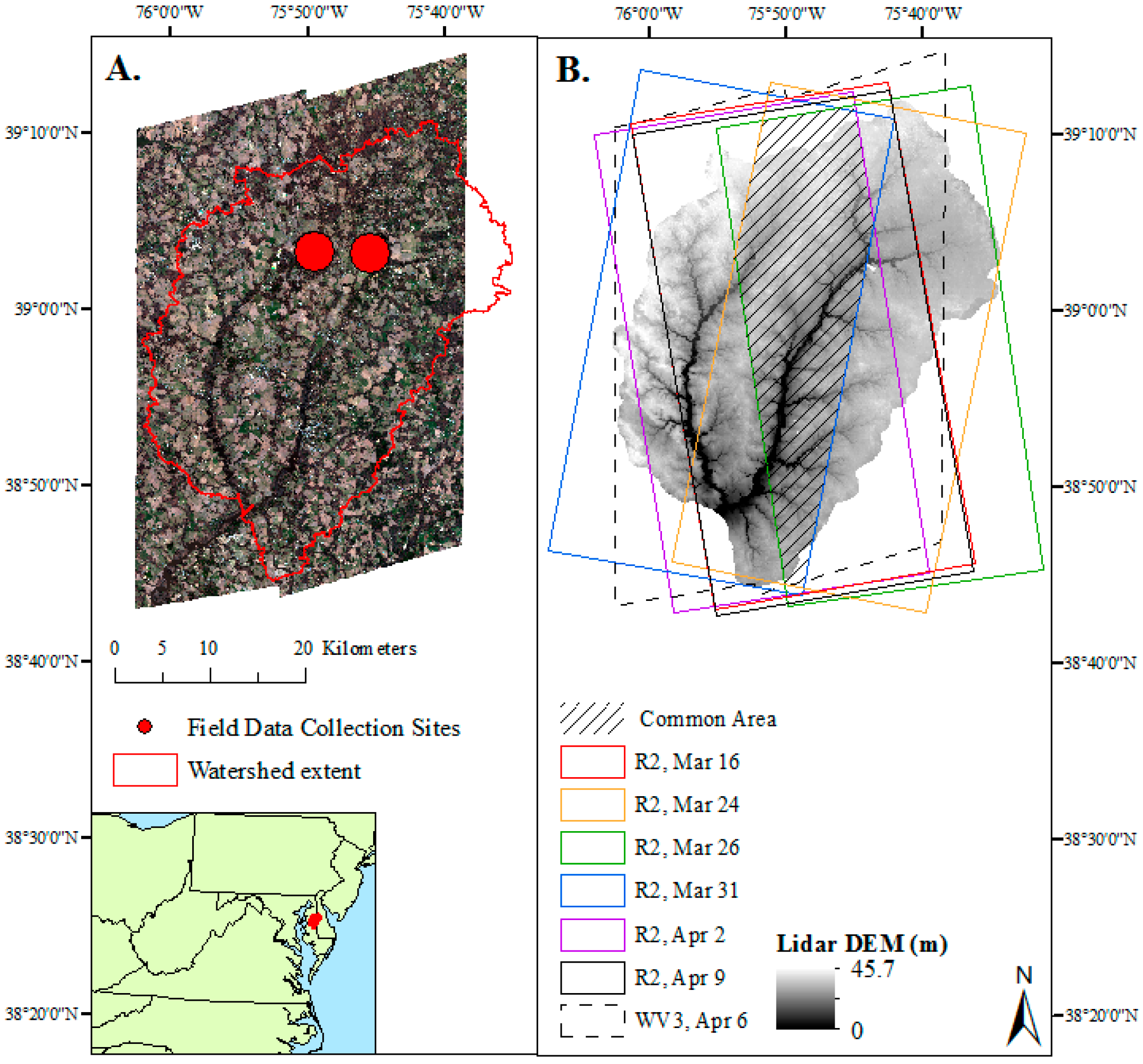
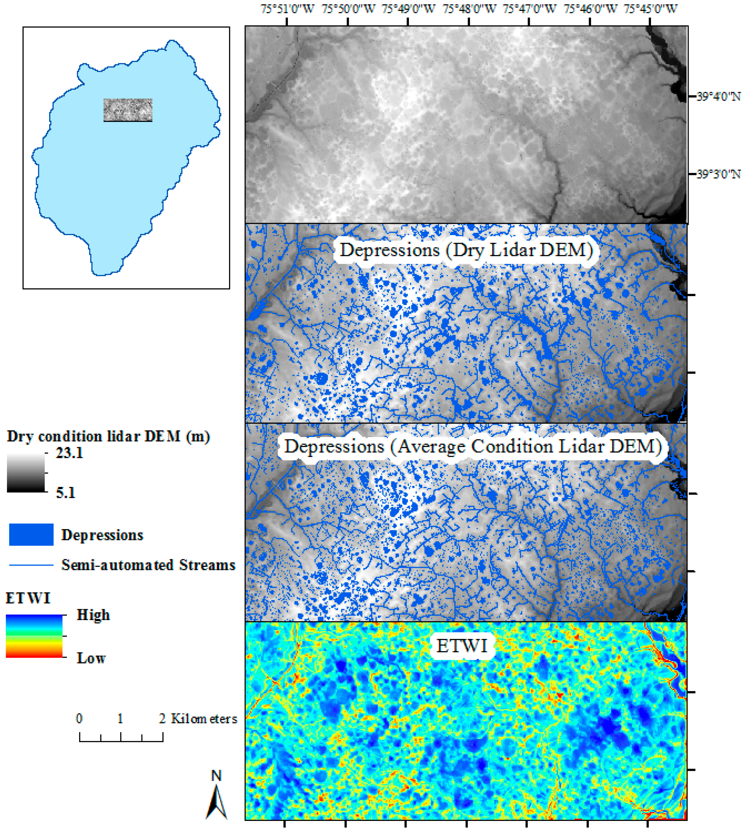
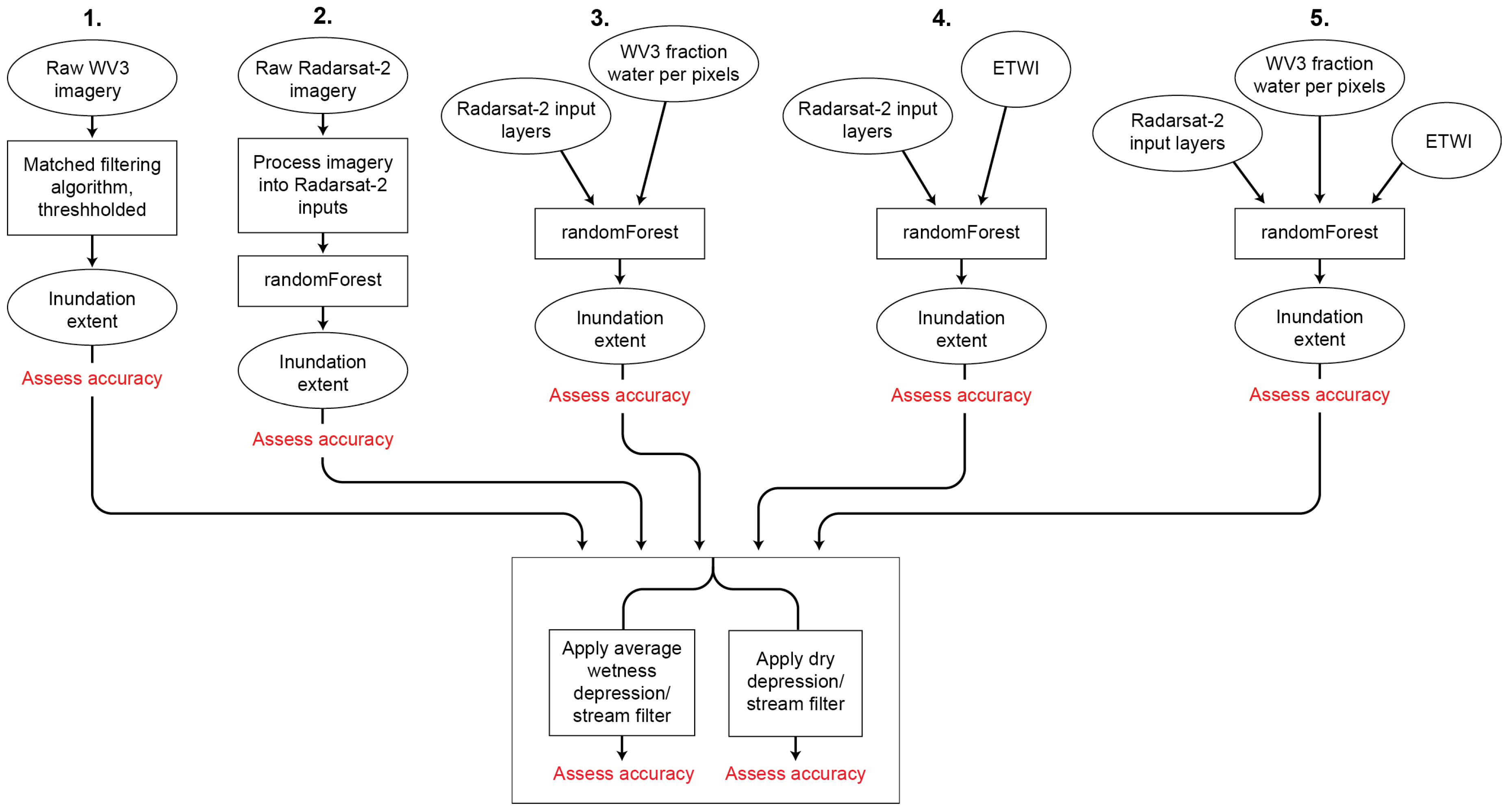
19], however, only efforts using lidar backscatter intensity have attempted to map surface water at the scale of individual wetlands. In this study, we sought to maximize the accuracy of forested inundation maps across the Upper Choptank River watershed in the Delmarva Peninsula by testing if accuracy could be improved by integrating multiple datasets with unique advantages and incorporating a more sophisticated topographic measure (i.e., depression locations). We tested the ability of Radarsat-2, Worldview-3, lidar-derived depressions, and a topographic wetness index (TWI) derived from a lidar DEM, to map surface water extent. Our research questions included:
  • How do prior weather conditions affect the identification of depressions using lidar data?
  • How accurate are inundation products derived using high-resolution optical and SAR data?
  • How consistent is the accuracy of inundation products derived from SAR data repeatedly collected over a short time period?
  • Can integrating multiple sources of data (lidar, optical, and radar imagery) improve inundation mapping?
Our study was designed to evaluate the contribution of each of the datasets in improving the accuracy of mapping forested inundation during spring high-water conditions. We are unaware of any studies that have paired these sources of imagery with lidar-derived depressions. Accurate mapping of inundation is critical to predicting and monitoring the effects of human-induced change and interannual variability on water quantity and quality.

2. Methods

2.1. Study Area

Inundation was mapped across the Upper Choptank River watershed (123,730 ha), defined as upstream from the intersection of the Tuckahoe Creek and the Choptank River, on the Delmarva Peninsula in eastern Maryland and Delaware. The Delmarva Peninsula is within the Outer Coastal Plain and the Upper Choptank River watershed is predominantly characterized by poorly drained soils on floodplains and well-drained soils in the uplands. Sediments of the surficial aquifer are primarily sand and gravel and the surficial aquifer is unconfined [47]. Land cover within the study area is dominated by cultivated crops (45%), woody wetlands (20%), hay/pasture (14%), and deciduous forest (10%) [48]. Much of the watershed has been hydrologically modified to accommodate agriculture, leaving the primary types of wetlands found within the watershed to be wetland depressions (e.g., Delmarva bays) and wetland flats, as well as riparian wetlands. Average weather conditions were derived from National Oceanic and Atmospheric Administration (NOAA) weather stations within and adjacent to the study area. Long-term (1950–2014) summer (June–August) temperatures average 23.6 °C, while winter (December–February) temperatures average 2.2 °C. Winter precipitation averages 7.9 cm per month while summer precipitation averages 11.2 cm per month. The 2014–2015 winter prior to the image collection was slightly colder and wetter than average (0.6 °C average temperature and 10.2 cm precipitation per month).
In this analysis, several datasets were evaluated for inundation mapping over small, forested wetlands across the study area. Topographic depressions were derived from two different lidar datasets, one collected during dry conditions and the second collected during average wetness conditions. Inundation extent was mapped using: (1) Radarsat-2 imagery collected on six dates within a three-week period; (2) Worldview-3 imagery; and (3) Radarsat-2, Worldview-3, and an enhanced topographic wetness index. The topographic depressions were merged with a stream dataset and were used to filter the inundation maps to reduce commission errors. A list of the products used in the analysis and their sources is provided in Table 1.

2.2. Field Data Collection

Field data were used to derive training and validation datasets of inundated and non-inundated points. Field data were collected on 16, 17, 24, 25, and 31 March 2015, as well as 1 and 6 April 2015 on two Nature Conservancy properties, one located east of Tuckahoe Creek and the other just west of the main stem of the Choptank River (Figure 1). The field effort was designed to coincide with the Radarsat-2 and Worldview-3 satellite flyover dates. Multiple two-person teams created polygons of inundated and non-inundated areas using global positioning systems (GPS) units. Non-inundated polygons were at least 20 m from the edge of an inundated area. A total of 12.8 ha (73 polygons) of forested, inundated area and a total of 4.4 ha (34 polygons) of forested non-inundated area were recorded. The polygon dataset was co-registered to a lidar DEM using tie points.

2.3. Lidar Processing

2.3.1. Lidar DEMs

In this study we used lidar DEMs collected under both average and dry (i.e., very minimal surface water) wetness conditions to map surface depressions. We also utilized previously published datasets derived from lidar DEMs including a stream dataset and an enhanced topographical wetness index. Both lidar DEMs were calculated from the adjusted bare-earth lidar point files using inverse distance weighted interpolation. The first lidar DEM covered the entire Upper Choptank River watershed and was created from three separate lidar data collection efforts (April–June 2003 (vertical accuracy root mean square error (RMSE) = 14.3 cm) and March–April 2006 (vertical accuracy RMSE = 18.5 cm) for Maryland (1-m resolution) and April 2007 (vertical accuracy RMSE = 18.5 cm) for Delaware (3-m resolution)) [49]. The 1-m and 3-m resolution DEMs were resampled to 2-m resolution. The lidar data within Maryland was collected for the Maryland Department of Natural Resources (metadata hosted online: http://dnrweb.dnr.state.md.us/gis/data/lidar/). The lidar data within Delaware was collected as part of the 2007 Delaware Coastal Program Lidar initiative (metadata hosted online: https://data.noaa.gov/harvest/object/7418610c-3842-4671-9040-1bac0faf9372/html). These datasets were designed to meet or exceed the Federal Geographic Data Committee’s National Standards for Spatial Data Accuracy for data at 1:2400. Horizontal positional accuracy of point returns was estimated to be 50 cm or better. The second lidar dataset was collected on 24 December 2007 over a subset of the watershed (~10.7 km × 5.1 km, 3 m resolution). The vertical accuracy of the dataset had a RMSE of 15 cm. The near-infrared lidar returns had a pulse rate of 126,000 Hz and scan frequency of 50 Hz [46]. Although coarser in derived spatial resolution, the original pulse density was higher for the December data collection (~2.8 points·m−2) than the previous effort (~1.4 points·m−2).
One limitation of mapping depressions using lidar DEMs is that near-infrared lidar returns over water typically reflect the elevation of the water surface instead of the elevation of the ground below it [3]. This implies that antecedent water conditions can influence the mapping of depression extent using lidar data. The two lidar DEMs used were collected under different wetness conditions. The first lidar DEM (2003–2007) represented near normal or average wetness conditions. Palmer Hydrological Drought Index (PHDI) ranged from −1.8 to 3.6 and averaged 1.4 across the dates [50] and the data were collected in the spring, a seasonally wet period. The second lidar DEM represented dry conditions. The PHDI averaged −3.1, classified as a severe drought. In addition, it was collected at a time of year in which minimal water is typically present in wetlands. The wetness condition is relevant as it can influence surface water elevation values.

2.3.2. Depression Identification

Depressions were identified using the Stochastic Depression Analysis Tool in Whitebox GAT, an open-source software [51], largely following methods by Wu et al. [36]. The Depression Analysis Tool aims to separate out erroneous artifacts in the DEM from “true” depressions. Prior to analysis both lidar DEMs were subdivided into sub-watersheds to reduce processing time. We used a Gaussian probability function (mean = 0, RMSE = 18.5 cm for the average wetness condition DEM and RMSE = 15 cm for the dry DEM) to derive a normal distribution of potential error values. A modified version of the turning bands simulation technique [52] was then used to introduce spatial autocorrelation into the potential error values [53]. In each iteration, a random sample from the potential error values was added to the original DEM prior to depressions being filled and identified using Wang and Liu’s [54] depression filling technique. Changes in the number of depressions identified were tested up to 50 iterations, but were found to stabilize after 20 iterations. Cells were considered part of a depression if identified as such in 80% of the iterations [36]. An edge preserving smoothing filter with a window size of 3 × 3 was applied to reduce within depression speckling. Depressions with an area smaller than 50 m2 were removed. Lastly, to improve our confidence that depressions represented water features, only depressions that overlapped with surface water extent, defined as any inundated pixels, as identified by the Worldview-3 water classification, were retained. This step was meant to reduce errors of commission, but could have resulted in an underestimation of wetland features, particularly features that store water for short periods of time.

2.3.3. Depression/Stream Filter

The two depression outputs (representing dry and average wetness conditions) were each combined with a semi-automated stream dataset also derived from the average wetness condition lidar DEM [49]. This stream dataset has been shown to be more comprehensive and accurate relative to the U.S. Geological Survey National Hydrography Dataset (NHD) high-resolution stream dataset [46]. The semi-automated streams were buffered by 2 m to account for stream and riparian width. Stream/River polygons provided by the NHD high-resolution dataset were also included to account for stream width in the Choptank River and other large river features within the watershed. The depressions, buffered streams, and stream/river polygons were merged together to create (1) an average wetness condition depression/stream dataset and (2) a dry condition depression/stream dataset.

2.3.4. Enhanced Topographic Wetness Index

The enhanced topographic wetness index (ETWI) was derived from the dry lidar DEM (3-m resolution) [46]. First, a topographic wetness index (TWI) was derived using the equation: ln(a/tanβ), in which “a” represented the upslope contributing area per unit contour length and “β” was the local slope [55]. Using the open-source software program System for Automated Geoscientific Analysis (SAGA) v. 2.0.8, the FD8 flow routing algorithm [56] was calculated from the DEM and applied to the SAGA Wetness Index module [57], to create the FD8 TWI layer [46]. ArcGIS was then used to create a local terrain normalized relief (LTNR) map that was added to the FD8 TWI layer to produce an enhanced topographic wetness index (ETWI), where FD8-based wetness index values within identified depressions were increased by 10% [46]. The continuous values for LTNR and ETWI were then qualitatively thresholded into four classes of wetland and upland predictive strength and added together to produce a final relief-enhanced topographic wetness index (referred to as ETWI) [46]. The spatial variability of the ETWI values in relation to the lidar-derived depressions is shown in Figure 2.

2.4. Inundation Mapping and Assessment

2.4.1. Worldview-3 Processing

Worldview-3 imagery (8-band) was collected across the watershed on 6 April 2015 and delivered as nine separate images (Table 2). Data processing was performed using the ENVI software package (Exelis Visual Information Solutions, Inc., Herndon, VA, USA). The imagery was atmospherically corrected and converted to ground reflectance using Fast Line-of-sight Atmospheric Analysis of Hypercubes (FLAASH) [58,59]. A minimum noise fraction transformation was applied to the spectral bands to reduce noise or random distortion in the data [60]. The Matched Filtering algorithm was used to calculate the fraction water within each pixel. This algorithm is based on well-known signal processing methodologies [18]. It is designed to detect the abundance of a known endmember (e.g., water) against a composite of unknown background endmembers (e.g., vegetation, soil, etc.) using a partial unmixing technique [18,61]. The algorithm is similar to Spectral Mixture Analysis, but the major advantage of this technique is that it does not require signatures for other endmembers present in the image and instead maximizes the response to a single user-defined endmember [18]. The spectral signature was derived from open water features within both forest and non-forest cover types across each image. The output values (fraction water within each pixel) were then linearly stretched to enhance the data by maximizing the spread of pixel values. A Frost filter with a window size of 3 × 3 was applied to further improve the coherency of output and reduce within feature speckling. The imagery was co-registered to the lidar DEM using tie points. Pixels with a water per-pixel fraction of >0.25 were classified as inundated. Lastly, the Worldview-3 output was resampled to 5.6 m resolution using cubic convolution so that the accuracy statistics were directly comparable to the Radarsat-2 and integrated model outputs.

2.4.2. Radarsat-2 Processing

Fine resolution, quad-polarization Radarsat-2 imagery were acquired on 16, 24, 26, and 31 March, as well as 2 and 9 April 2015 across the study area in Single Look Complex (SLC) data format. Specific details regarding the Radarsat-2 image acquisitions are included on Table 2. A flowchart of the Radarsat-2 processing steps is shown in Figure 3. The Radarsat-2 images were processed using PCI Geomatica’s SAR Polarimetric Workstation. Digital number values were converted to Sigma Naught or backscattering coefficient with units of decibels for analysis [62]. The SLC quad-polarization data, which represents complex data, were extracted to a 3 × 3 covariance matrix, which averages the cross-polarization backscatter, and allows the polarization intensities (HH, VV, and HV) to be extracted for further analysis [63]. Three decompositions were applied to the covariance matrix including the Cloude–Pottier [64], Touzi [65] and Freeman–Durden [66] decompositions. The polarimetric decomposition of fully polarized data can help maximize the ability of SAR data to distinguish physical features on the ground [67,68]. These decompositions were selected as they have all previously been found to be helpful when mapping surface water [65,67,68,69]. The SLC data were also extracted to the normalized Kennaugh scattering matrix [69]. As explained in Schmitt et al. [70], the traditional Kennaugh matrix is the linear transformation of the four-dimensional Stokes vector, which consists of the total intensity (K0) and 15 linear coefficients of the transformation. This approach directly interprets and scales the backscattering matrix elements themselves, deriving total intensity, as well as elements related to absorption, diattenuation, and retardance [69]. This approach has been found to optimize detection of surface water under vegetation [69,70]. The normalized Kennaugh matrix (k) was derived by dividing the Kennaugh matrix by the total intensity (I), so that all elements range between −1 and 1.
[ K ] =   [ K 0 K 4 K 5 K 6 K 4 K 1 K 9 K 8 K 5 K 9 K 2 K 7 K 6 K 8 K 7 K 3 ]   = I   ·   [ 1 k 4 k 5 k 6 k 4 k 1 k 9 k 8 k 5 k 9 k 2 k 7 k 6 k 8 k 7 k 3 ]   = I · [ k ]
The Polar Lee Adaptive Filter was applied to the covariance matrix and normalized Kennaugh matrix outputs with a window size of 5 × 5 to reduce noise, but preserve edges. Output rasters were resampled to 5.6 m resolution using cubic convolution to ensure identical cell resolutions between image dates and co-registered to the lidar DEM using tie points. The mathematical details of these procedures are provided in Schmitt and Brisco [69] and Touzi et al. [65].
Differences in vegetation structure between forest and non-forest land cover types influence the SAR backscatter signal from water [71,72]; therefore separate models were derived for forest and non-forest cover types for each of the six dates. Forest extent was defined using the 2011 National Land Cover Dataset [48] as deciduous forest, evergreen forest, mixed forest, and woody wetlands. Forested and non-forested inundation models were clipped to the NLCD defined forest and non-forest extent, then merged into a single inundation extent map. For the forested models training points were randomly selected using the field data collection and raw Worldview-3 imagery (535 non-inundated points, 502 inundated points). For the non-forested models, these points were randomly selected using the raw Worldview-3 imagery (904 non-inundated points, 923 inundated points). The same training points were utilized for each of the six image dates.
To classify the images into inundated/non-inundated, we derived 500 binary trees or bootstrap iterations using out of bag (OOB) samples (70% of points used to train, 30% of points used to validate) in the random forest model as implemented in R [73], with the spatial component implemented in R using ModelMap [74]. Random forest models are generally insensitive to collinearity among metrics, however the inclusion of correlated variables can deflate both variable importance and the overall variation explained by the model, while the inclusion of a large number of variables can make interpretation difficult and introduce noise [75]. We implemented variable selection using random forests in R (varSelRF package), which uses backwards variable elimination and selection based on the importance spectrum to select the smallest number of non-redundant variables [76]. We ran an initial random forest model with all variables, then a revised model that only included variables selected by varSelRF. Accuracy statistics were generally improved by using the subset of variables; therefore, the inundation maps were derived using the subset of variables, listed in Table 3. A random forest model was derived in R for each Radarsat-2 date.

2.4.3. Integrated Inundation Mapping

To evaluate potential improvement in accuracy using multiple sources of imagery, we ran random forest models with multiple data types and compared the accuracy of output inundation maps with those derived using Radarsat-2 or Worldview-3 alone. Combinations tested included (1) Radarsat-2 input rasters and the Worldview-3 water fraction raster; (2) Radarsat-2 input rasters and the ETWI raster; and (3) Radarsat-2 input rasters, the Worldview-3 water fraction water raster and the ETWI. For Radarsat-2 we used the 9 April 2015 Radarsat-2 input rasters because the date of image collection was closest to that of the Worldview-3 imagery (6 April 2015). As the ETWI was only available for a subset of the watershed, the combined models were only created for this same spatial subset (Figure 2). These combined models were only run for the NLCD-forested cover area as that was the focus of the analysis.

2.4.4. Accuracy Assessment

Accuracy statistics were produced to compare the quality of the various inundation maps produced (Figure 4). Accuracy statistics were derived using an independent set of data points, not used in the random forest models, but also derived from the field data collection effort. Each forested model was validated using 200 inundated points and 200 non-inundated points restricted to forested cover types. Each non-forested model was validated using 200 inundated points and 200 non-inundated points restricted to non-forested cover types. As the analysis was focused on forested cover types, accuracy metrics for non-forested inundated extent were presented only per Radarsat-2 date and only for comparative purposes. The validation points were randomly selected from the non-inundated and inundated field-collected polygons with a minimum distance of 6 m apart and used to validate each of the models.
The accuracy of the inundated extent maps was quantified using the imagery alone (i.e., Worldview-3, Radarsat-2, or combined models) and after testing two versions of the depression/stream filter (Figure 4). Each inundated map was converted to a shapefile and filtered so that inundated polygons were retained if they overlapped (1) streams or average wetness condition depressions or (2) streams or dry condition depressions. Accuracy was reassessed after applying each of the filters and compared to the original inundated extent map. Accuracy metrics presented included overall accuracy, omission error, commission error, Dice coefficient, and relative bias. Omission and commission errors were calculated for the category “inundated”. The Dice coefficient is the conditional probability that if one classifier (product or reference data) identifies a pixel as inundated, the other one will as well, and therefore integrates omission and commission errors [77,78]. The relative bias provides the proportion that inundated area is under or overestimated relative to the inundated area of the reference product [79]. McNemar’s chi-squared test with continuity correction was used to test for significant differences between different inundation maps, as recommended by Foody [80]. We note that although statistical significance for changes between maps are presented, it may or may not be relevant to users. Percent reductions in error and improvements in the visual quality of the map may instead be of equal value to users.

3. Results

3.1. Impact of Wetness Conditions on Lidar-Based Depression Identification

The inundated topographic depressions were found to occur disproportionately in forested NLCD land cover types. Although forested NLCD land cover types (woody wetlands, deciduous, mixed or evergreen forest) comprise only 32.1% of the watershed, 65.4% of the lidar-derived depressions by count and 44.9% of depressions by area (lidar collected under average wetness conditions) were found to occur within forested cover types. Note that the non-forested cover is heavily modified, dominated by cultivated crops (44.7%), hay/pasture (13.9%), and developed/barren (6.5%). We compared the abundance and total area of depressions derived from lidar DEMs, where the lidar was collected under dry and average wetness conditions. More depressions by count (38%) and by area (39%) were identified using the dry condition lidar DEM relative to the average wetness condition lidar DEM (Table 4). This finding is logical as wetness conditions can influence surface-water elevation. Depressions full of water at the time of the lidar data collection may not be identified as a depression if no elevation change exists between the full depression and the adjacent non-inundated area. By contrast, if the same depression is empty at the time of the lidar data collection it will likely be identified as a depression. Visually, the dry condition lidar DEM identified both new depressions as well as expanded extents for depressions relative to the average wetness condition lidar DEM (Figure 2 and Figure 5).

3.2. Accuracies of Inundation Products Derived Using Different Data Sources

Overall accuracy within forested cover across the six Radarsat-2 dates with no filter applied averaged 73.3%, while omission and commission errors for detecting inundation averaged 26.6% and 26.4%, respectively (Table 5). Unfiltered Radarsat-2 maps of inundation were found to be statistically similar, except for 9 April which was found to be significantly different (Figure 6). The error rates can be compared to error rates in mapping inundation within non-forested cover types with Radarsat-2 which averaged 7.9% and 4.7% errors of omission and commission for inundation, respectively (Table 5). Both the number and variety of variables selected for inclusion in the Radarsat-2 random forest models varied between each of the six dates. Element 1,1 of the covariance matrix (ShhS*hh) was the only variable included in all six models (Table 3). Five of the six dates included elements from the Kennaugh scattering matrix and the Touzi decomposition, while four of the six dates included elements from the Freeman–Durden and Cloude–Pottier decompositions (Table 3). When evaluating relative variable importance as indicated by the decrease in node impurity (Gini importance), an element of the Kennaugh scattering matrix, Element 1,1 of the covariance matrix (ShhS*hh) and the Dominant Touzi Alpha S Parameter were consistently among the most important variables across the six dates.
At the scale of the watershed, Worldview-3 produced a coherent pattern of inundation (Figure 7). However, the distribution of the per-pixel fraction of water suggests that classifying pixels with less than 100% water as inundated was a critical component of accurately capturing inundation patterns (Figure 8). In evaluating the accuracy of Worldview-3, the inundation map produced a higher overall accuracy (+17.3%) than Radarsat-2 imagery (Table 6), but because differences in the two maps were similar in disagreement between inundated/non-inundated and non-inundated/inundated, no statistical difference was found using McNemar’s chi-squared test of significance, despite a strong visual improvement in the mapped inundation (Figure 9).

3.3. Effectiveness of Multi-Source Data Integration for Inundation Mapping

Applying a filter based on the lidar-derived depressions (average wetness conditions) to forested inundation extent improved overall accuracy of Radarsat-2 by 5.4% across the six Radarsat-2 image dates as a result of slightly increasing water omission errors (1.0%) but substantially reducing water commission errors (−7.8%) (Table 5, Figure 7). For Worldview-3, although the depression filter provided visual improvement (Figure 7), the reduction in commission error (3.8%) was balanced by an increase in omission error (4.5%). The post-filter versions of both the Radarsat-2 and Worldview-3 inundation maps were found to be significantly different from the pre-filter versions.
Applying the low-water lidar-derived depressions, relative to the average wetness condition lidar-derived depressions for Radarsat-2 resulted in, on average, a slightly lower omission error but slightly higher commission error, resulting in no consistent improvement in overall accuracy across the six dates and no change to accuracy of the Worldview-3 inundation map (Table 5 and Table 6). These findings suggest that utilizing a depression layer can improve inundation maps by reducing errors of commission. Although antecedent conditions influence mapped depressions, it may have minimal effect on improving inundation maps. This finding may not be true in other landscapes but is highly relevant as dry condition DEMs are often not available.
Errors of omission in detecting inundation after filtering outputs using the average wetness condition lidar-derived depressions ranged from 20.5% to 30.5%, while errors of commission ranged from 11.7% to 25.5% (Table 5). These error rates indicate that even after applying depression filters, a substantial amount of error remained in the Radarsat-2 surface water maps within forested cover (Figure 7). By integrating Worldview-3 with Radarsat-2 and the ETWI, within-feature speckling was reduced and a more visually coherent (Figure 7 and Figure 9) and significantly more accurate (Table 6) inundation extent map was produced. In the random forest models that considered Radarsat-2, Worldview-3 and ETWI inputs, the probability of surface water as determined by Worldview-3 was consistently the most important variable. Elements from the Kennaugh matrix, covariance matrix and Touzi decomposition were also found to be important, as was the ETWI input (Figure 10). Interestingly, integrating ETWI with Radarsat-2 reduced the accuracy of the models, but adding ETWI to Radarsat-2 and Worldview-3 improved accuracy, although it was not found to be significantly different from maps of inundation derived using Radarsat-2 and Worldview-3.

4. Discussion

Our ability to map surface-water extent is unequal across the landscape. Monitoring surface-water extent in landscapes dominated by large, non-forested water bodies is limited primarily by the temporal frequency and date range of the available imagery. Monitoring surface-water extent in landscapes dominated by small wetlands and/or forested environments, also requires consideration of imagery spatial resolution as well as our ability to “see” through tree trunks, branches and leaves. The development of improved techniques to map surface-water extent in these challenging environments is key not only to improve our ability to monitor variability in surface-water extent, but also to improve our understanding of wetland location. National Wetland Inventory (NWI) maps, produced by U.S. Fish and Wildlife Services, for example, are the most widely available and used wetland maps in the United States. As NWI wetlands were visually interpreted from aerial photography, errors are highest for wetland types that are difficult to detect with photointerpretation such as small, forested wetlands, farmed wetlands, partly drained wetlands, or wetlands in narrow valleys [81,82]. Our approach could be applicable to update the NWI dataset, particularly in regions dominated by deciduous forests. In this study we explored how prior weather conditions influenced depression identification from lidar data, how accurate and consistent inundation products were derived using high-resolution optical and SAR data, and if integrating multiple sources of data (lidar, optical, and radar imagery) could improve inundation mapping.
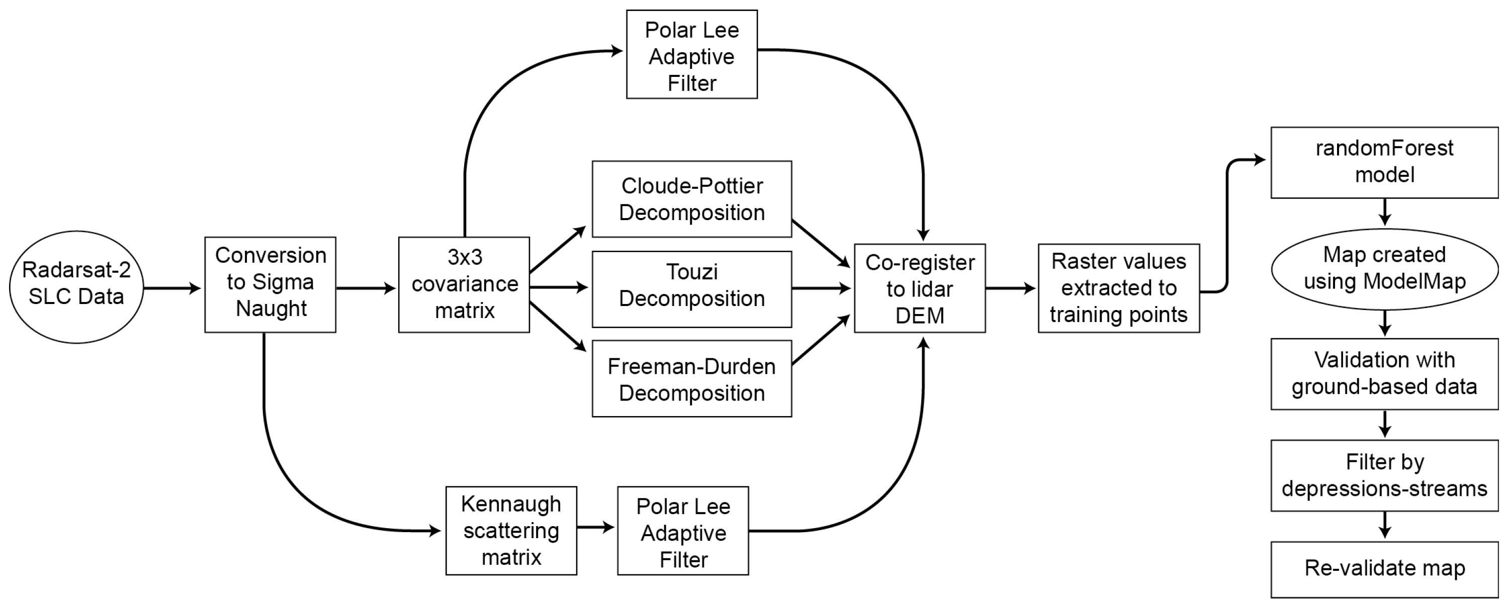
Within our analysis, we used Radarsat-2 imagery as our primary source of imagery because SAR has been previously shown to be effective in mapping surface water under vegetated canopies [24,25,26]. Future efforts to monitor inundation in forested areas during the growing season will likely require SAR imagery. We found that Radarsat-2 alone can produce adequate maps of inundation in a challenging environment dominated by small, forested wetlands. When paired with a lidar-derived filter of depressions and streams, Radarsat-2 inundation maps showed an average, overall accuracy of 79%. In comparison, Pistolesi et al. [28], who similarly mapped small, forested wetlands using ALOS PALSAR data, obtained an overall accuracy of 67% to 72%, while Lang and McCarty [46] mapped forested, inundated cover in an overlapping study area within the Upper Choptank River watershed at 66% accuracy using leaf-off, near-infrared digital photography.
Lang et al. [27] mapped forested wetlands in the Chesapeake Bay watershed using Advanced Synthetic Aperture Radar (ASAR) imagery and detected inundation during leaf-off conditions 89% to 96% correctly. These accuracy statistics are substantially better than that achieved using Radarsat-2 alone in this study. The imagery utilized by Lang et al. [27] was collected at an incidence angle of 23°, which may partially explain differences in findings. The incidence angle is an important consideration in the utilization of SAR imagery to map surface water below vegetation. The community has not reached agreement as to how large of an incidence angle is acceptable, but the smaller the angle, or closer to nadir, the fewer leaves and branches the radar signal has to travel through to reach the surface. Although our incidence angles can be considered less than ideal (31.4°–48.0°), it is similar to the incidence angles used by others to detect surface water [69,83,84], however wetland size may matter and most of these existing efforts targeted open water wetlands or larger flooded vegetation features.
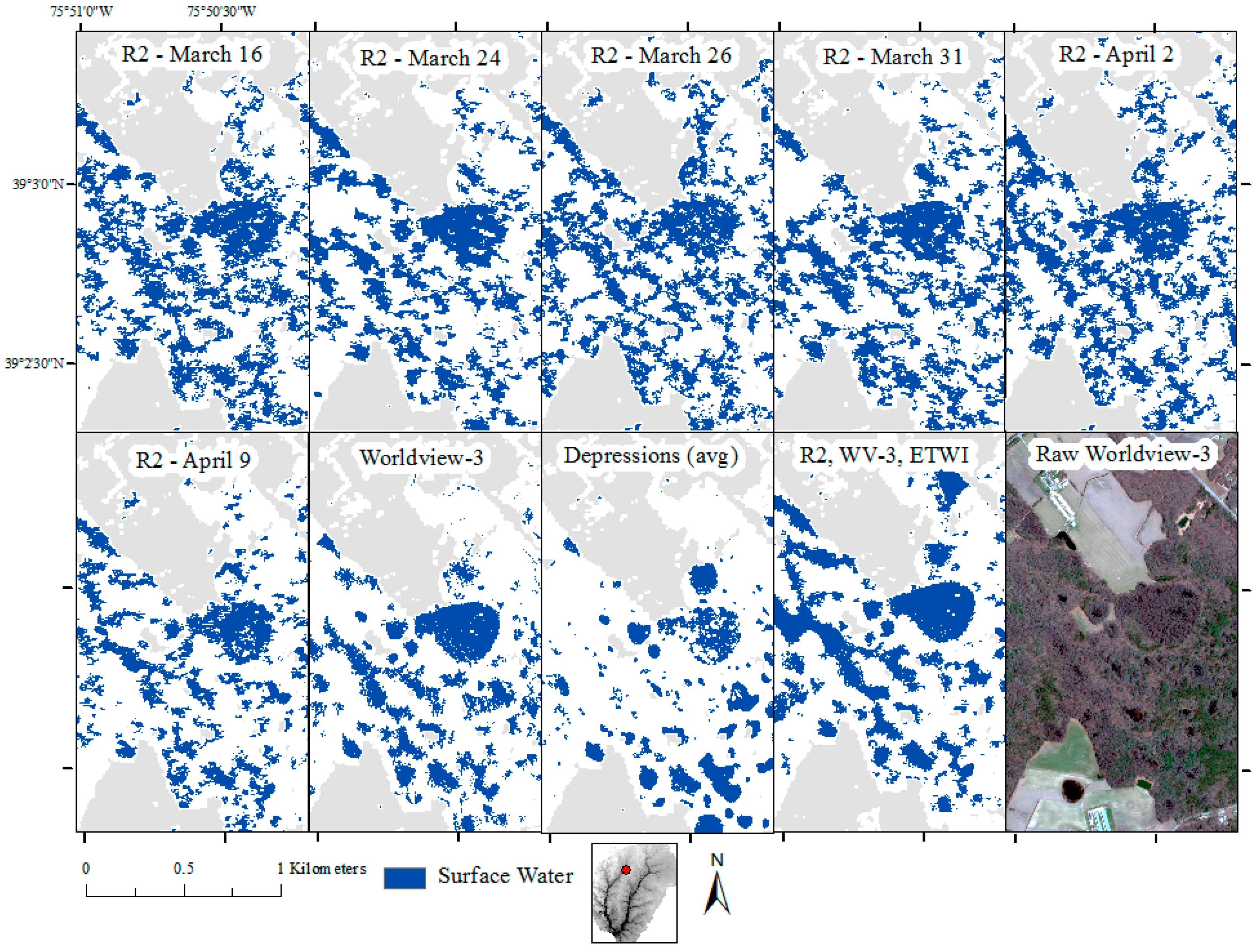
Several other sources of error may have also influenced our accuracy results. Antecedent precipitation conditions may have negatively impacted the Radarsat-2 surface water maps. Recent precipitation can reduce the contrast in signal between flooded forest and adjacent non-flooded forest by elevating soil moisture levels in non-flooded forest. Precipitation occurred in the seven days prior to all six of the Radarsat-2 images and occurred in the two days prior to four of the six Radarsat-2 images (Table 1). This may help explain the large amount of error observed in the March 16 surface water output which saw 2 cm of precipitation fall within the two days prior to the image collection (Table 1). This image was also collected within days of snowmelt, meaning soil moisture content was likely high even in upland areas. Antecedent precipitation conditions could also help explain some significant differences in inundation mapped by Radarsat-2 on different dates, a finding which suggests that subtle differences in image specifications and ground conditions can influence the ability of SAR to map inundation. It is also possible that wind, which can influence the surface roughness of water, could have negatively affected the Radarsat-2 inundation maps; however, we might expect wind to show a greater influence on open waters relative to forested waters. Efforts to maps inundation in non-forested areas showed a substantially higher accuracy relative to efforts to map inundation in forested areas (Table 4), suggesting that wind likely played a nominal role in influencing accuracy statistics. One additional potential source of error within the forested areas was that the training and validation data were largely collected across flooded forests with no gap in the canopy and non-inundated hummocks existed around tree trunks. These hummocks were often up to 1 m2, and may have introduced error into our reference points by overestimating inundation extent within the sampled “inundated” polygons and therefore potentially artificially elevated omission errors.
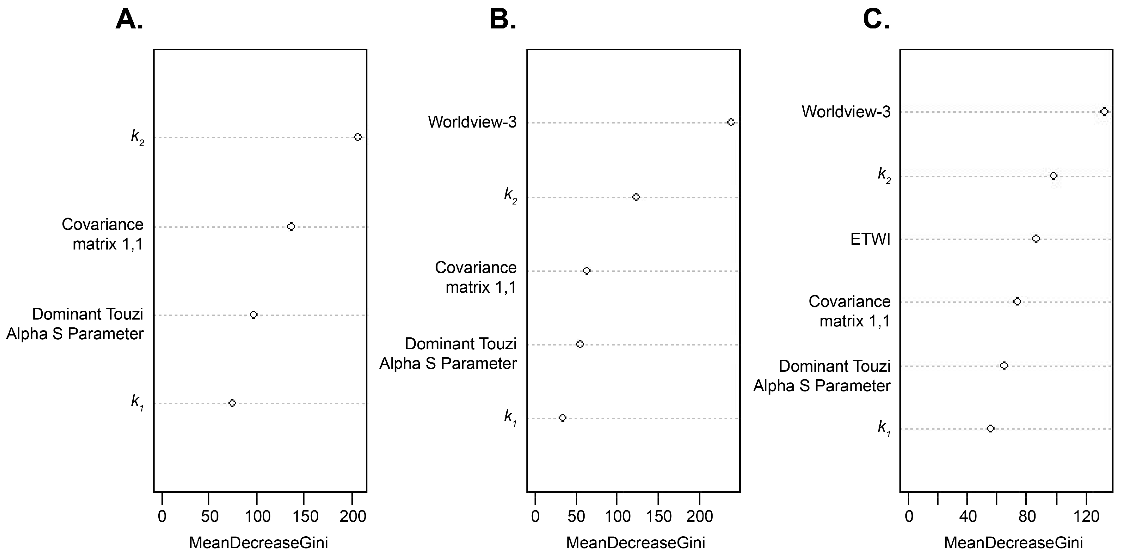
Approaches to effectively map inundation with SAR imagery are still developing. Decompositions and matrix transformations of raw SAR imagery have been found to be useful in mapping surface water [69,83,85]. The aim of this study was not to distinguish between the transformations that were more or less helpful, but instead to generate a number of inputs to maximize our probability of accurately identifying surface water with random forest models. However, large differences in the variables selected to be included between the six Radarsat-2 dates, suggest that it may be difficult to generalize, even within a single landscape, regarding which data transformations may be more or less helpful. In addition, variables selected for each date often included an element from several different decompositions and transformations, suggesting users should test a variety of methods instead of a single one when utilizing SAR imagery. The Kennough matrix was the most consistently utilized and tended to show the highest variable importance within random forest models across the six dates. This finding is consistent with several studies that have argued for utilizing this method [69,70].
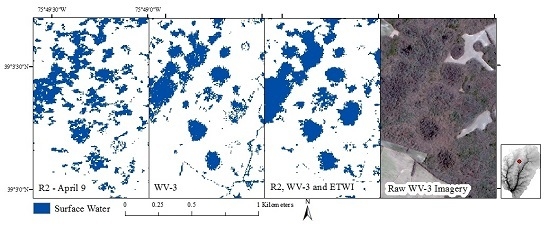
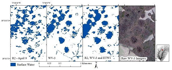
Integrating high-resolution imagery, in this case Worldview-3 imagery, was found to significantly improve inundation maps derived from SAR, in this case producing an overall accuracy of greater than 90%. However, timing, not just of the Radarsat-2, but also the Worldview-3 imagery collection is a critical component to interpreting our findings. The Worldview-3 imagery showed excellent potential to map forested wetlands and improved the ability of Radarsat-2 to map forested wetlands (combined models showed overall accuracy of 92% and 94%), however, our findings can be assumed to depend on collecting the imagery during leaf-off conditions. For applications focused on peak spring water conditions, this may be adequate, but for applications requiring seasonal changes in surface water extent, the ability of Worldview-3 imagery to perform following leaf-out is likely limited. Our strategy to improve mapping abilities by targeting leaf-off periods has been used by others (e.g., [19]), but is limited to environments which experience a leaf-off period. This means that our approach of integrating high-resolution multispectral imagery with SAR imagery will be less applicable to forests dominated by evergreen trees. In general, commercial satellites such as QuickBird-2, GeoEye-1, and Worldview-2 and 3, offer a very fine spatial resolution (1.2 to 2.4 m) that can improve the detection of small wetlands, narrow channels, and fine-scale changes in water level and surface water extent [11,22,86]. However, in addition to the need to target leaf-off seasons, imagery from these satellites is typically collected on-demand, and so may be costly or unavailable (due to competing requests for imagery) during a period of interest. Our analysis demonstrates that the utilization of such imagery during leaf-off periods can substantially improve the detection of surface water relative to using SAR imagery alone.
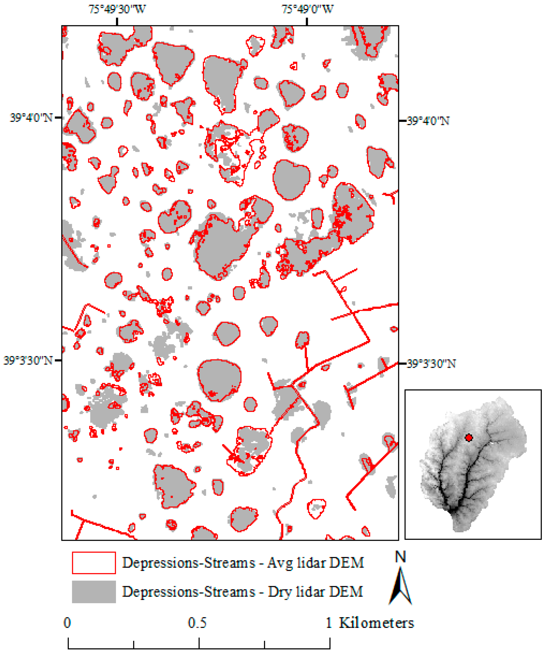
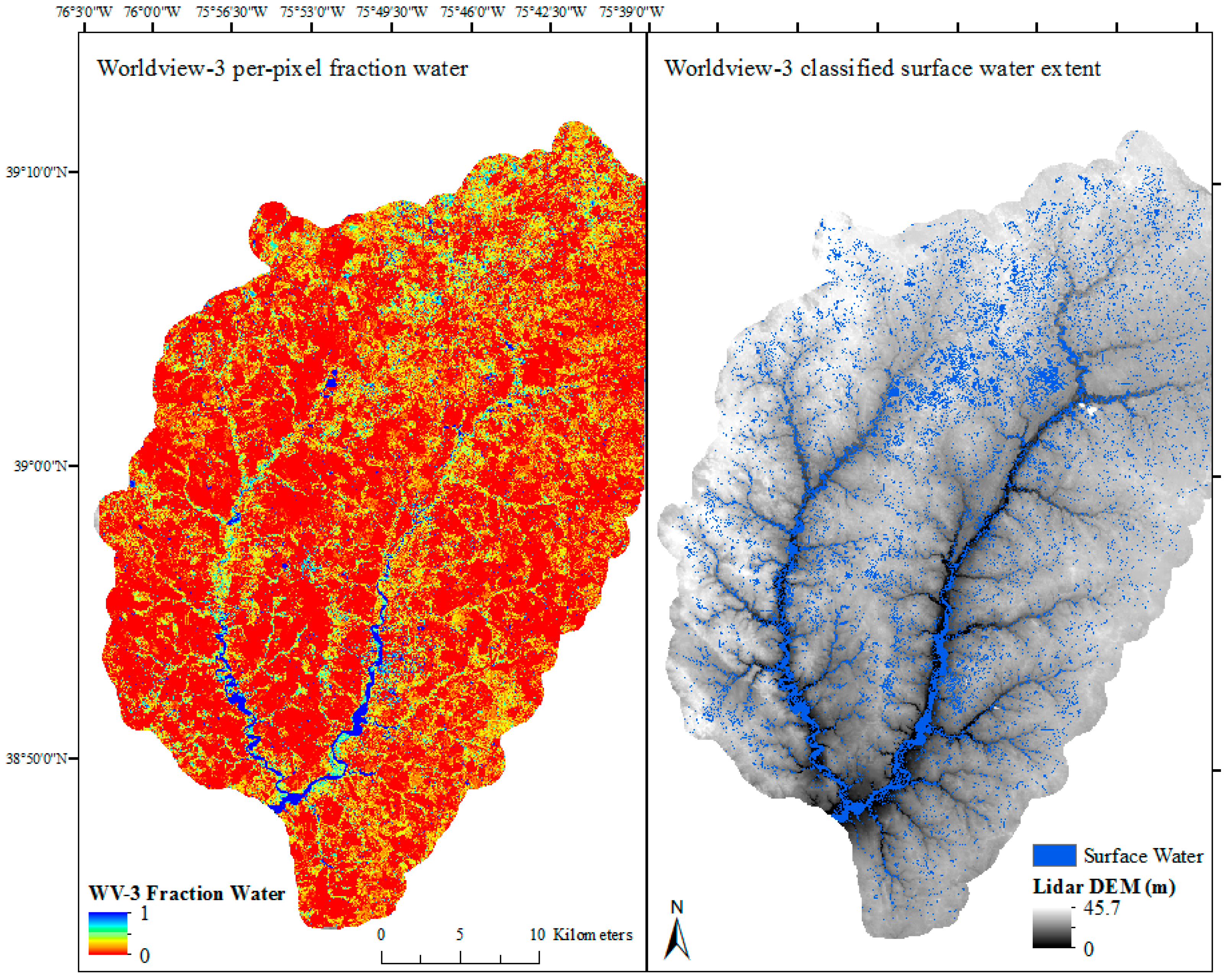
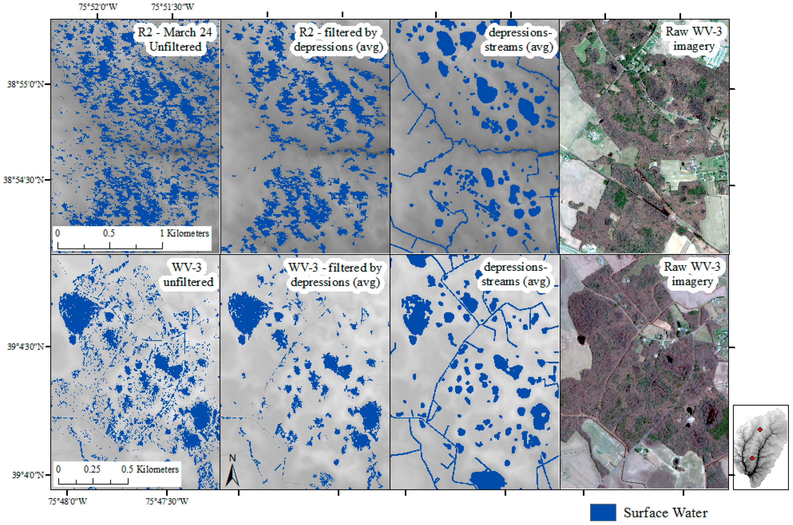
Alternatively, using lidar alone has been found to be highly effective to map inundation. Lang and McCarty [46] demonstrated that lidar intensity values can be very effective and accurate (97% of inundated points identified correctly) to map inundation in forested Delmarva bays. However, lidar coverage is currently not complete within the U.S. or globally, and observations from airborne lidar are often not repeated once a mission is flown, limiting its ability to be used for regular monitoring of inundation. In light of this, we tested if one-time lidar data collections could be used to improve inundation maps collected at a different point in time. Although antecedent weather conditions at the time of the lidar data collection substantially influenced the count and total area classified as depressions, we found they performed similar when used as a filter applied to inundation maps. Filtering inundation maps by lidar-derived depressions reduced errors of commission, improving overall accuracy of Radarsat-2 maps by 5% on average and suggests that lidar data collections collected at one point in time could be used to improve a time series of inundation maps. We note, however, that the depression filter cannot be expected to perform as well when mapping inundation in wetland flats, relative to wetland depressions, which may explain the small increase in omission errors we observed after applying the filter. In addition to deriving depressions, we also tested incorporating an ETWI, also derived from a lidar DEM. Although it did not improve the random forest model as much as incorporating Worldview-3 imagery, incorporating both Worldview-3 and the ETWI produced the best surface water models, a finding consistent with others [29,30,38] that topographic measures, in general, can improve efforts to map inundation.
The findings of this analysis are especially relevant as SAR imagery is rapidly becoming widely available. C-band SAR satellites, sponsored by the European Space Agency, have launched in recent years (Sentinel-1A was launched in April 2014, while Sentinel-1B was launched in April 2016). While others, such as the NASA-Isro Synthetic Aperture Radar (NISAR) satellite, a dual L-band and S-band satellite (launch planned for 2019–2020) are expected to become available in the near future. These satellites will provide continuous data collection at short return intervals and greatly improve our ability to map and monitor variation in surface water extent for forested wetlands. We hope that the approach presented here, which integrates SAR imagery with lidar DEMs and fine resolution imagery, can inform future efforts to utilize Sentinel and other satellites to detect surface water changes at greater spatial extents.

5. Conclusions

We evaluated the ability of Radarsat-2 quad polarization imagery and Worldview-3 imagery to map surface water extent in small, forested wetlands common across the Delmarva Peninsula. We also tested the ability of an ETWI and lidar-derived depressions to improve the accuracy of the surface water maps. We found that while Radarsat-2 alone produced adequate surface water maps, the outputs still contained a substantial amount of error. However, by integrating Worldview-3, in particular, as well as lidar-derived depressions and ETWI into the models, we were able to produce accurate surface water maps even in an environment as challenging as Delmarva bays. In addition, we found that the accuracy of inundation products derived from SAR varied even when collected over a few weeks, likely due to variability in antecedent moisture conditions. We found that antecedent moisture conditions also influenced our ability to identify depressions from lidar data; however, it had minimal influence on the effectiveness of using lidar-derived depressions to reduce commission errors. Accurate information regarding the extent and condition of terrestrial surface waters is essential to monitor and regulate aquatic ecosystems. Having effective methods to map surface water extent across challenging environments will help us to gain a better understanding of the human-induced and natural variation of surface water extent [87,88]. This study suggests that integrating SAR imagery with fine resolution multispectral imagery can improve surface water maps. It also suggests that lidar-derived depressions can be used to both improve confidence in and reduce error in surface water maps.

Acknowledgments

This work was funded by the U.S. EPA Office of Research and Development, National Center for Environmental Assessment (EPA-USGS IA-92410201-1, Multi-scale analyses and hydrologic simulation models of wetland-stream hydrologic connectivity in the Prairie Pothole Region). We would like to thank everyone who assisted in collecting field data for validation purposes. This includes Greg McCarty, Vincent Kim, Jason Todd, Laurie Alexander, Sergio Torres, and Derek Raisanen. Thank you also to the anonymous reviewers who provided valuable comments that helped improve the manuscript. Findings and conclusions in this presentation are those of the authors and the U.S. Geological Survey. They do not necessarily reflect the views or policies of the U.S. Fish and Wildlife Service. Any use of trade, firm, or product names is for descriptive purposes only and does not imply endorsement by the U.S. government.

Author Contributions

All authors made major and unique contributions. Melanie K. Vanderhoof is the primary author who designed the data processing procedures, processed the high-resolution imagery, oversaw the data processing and analysis, and wrote the manuscript. Di Ana Teresa G. Mendiola analyzed the Radarsat-2 imagery with assistance from Melanie K. Vanderhoof. Hayley E. Distler generated the lidar-derived depressions and analyzed the Radarsat-2 and mixed models. Megan Lang served as a technical advisor for the collection of the remotely sensed imagery and field data collection, and helped revise the inputs and analysis based on her extensive experience working within the watershed.

Conflicts of Interest

The authors declare no conflict of interest.

References

  1. Tiner, R.W. Geographically isolated wetlands of the United States. Wetlands 2003, 23, 494–516. [Google Scholar] [CrossRef]
  2. Winter, T.C.; Rosenberry, D.O. Hydrology of prairie pothole wetlands during drought and deluge: A 17-year study of the Cottonwood Lake wetland complex in North Dakota in the perspective of longer term measured and proxy hydrological records. Clim. Chang. 1998, 40, 189–209. [Google Scholar] [CrossRef]
  3. Lane, C.R.; D’Amico, E. Calculating the ecosystem service of water storage in isolated wetlands using lidar in North Central Florida, USA. Wetlands 2010, 30, 967–977. [Google Scholar] [CrossRef]
  4. Vining, K.C. Simulation of Streamflow and Wetland Storage, Starkweather Coulee Subbasin, North Dakota, Water Years 1981–98; Water-Resources Investigations Report 2002-4113; U.S. Geological Survey: Bismark, ND, USA, 2002; pp. 1–28.
  5. Yang, C.; Hao, Z.; Yu, Z.; Lin, Z.; Liu, S. Analysis and simulation of human activity impact on streamflow in the Huaihe River basin with a large-scale hydrologic model. J. Hydrometeorol. 2010, 11, 810–821. [Google Scholar] [CrossRef]
  6. Euliss, N.H., Jr.; Gleason, R.A.; Olness, A.; McDougal, R.L.; Murkin, H.R.; Roberts, R.D.; Bourbonniere, R.A.; Warner, B.G. North American prairie wetlands are important nonforested land-based carbon storage sites. Sci. Total Environ. 2006, 361, 179–188. [Google Scholar] [CrossRef] [PubMed]
  7. Poff, N.L.; Allan, J.D.; Bain, M.B.; Karr, J.R.; Prestegaard, K.L.; Richter, B.; Sparks, R.; Stromberg, J. The natural flow regime: A new paradigm for riverine conservation and restoration. BioScience 1997, 47, 769–784. [Google Scholar] [CrossRef]
  8. Horritt, M.S.; Di Baldassere, G.; Bates, P.D.; Brath, A. Comparing the performance of 2-D finite element and finite volume models of floodplain inundation using airborne SAR imagery. Hydrol. Process. 2007, 21, 2745–2759. [Google Scholar] [CrossRef]
  9. Chen, Y.; Huang, C.; Ticehurst, C.; Merrin, L.; Thew, P. An evaluation of MODIS daily and 8-day composite products for floodplain and wetland inundation mapping. Wetlands 2013, 33, 823–835. [Google Scholar] [CrossRef]
  10. Downing, D.; Nadeau, T.L.; Kwok, R. Technical and scientific challenges in implementing Rapanos “Water of the United States”. Nat. Resour. Environ. 2007, 22, 45–63. [Google Scholar]
  11. White, D.C.; Lewis, M.M. A new approach to monitoring spatial distribution and dynamics of wetlands and associated flows of Australian Great Artesian Basin springs using QuickBird satellite imagery. J. Hydrol. 2011, 408, 140–152. [Google Scholar] [CrossRef]
  12. Cohen, M.J.; Creed, I.F.; Alexander, L.; Basu, N.B.; Calhoun, A.J.; Craft, C.; D’Amico, E.; DeKeyser, E.; Fowler, L.; Golden, H.E.; et al. Do geographically isolated wetlands influence landscape functions? Proc. Natl. Acad. Sci. USA 2016, 113, 1978–1986. [Google Scholar] [CrossRef] [PubMed]
  13. Rains, M.C.; Dahlgren, R.A.; Fogg, G.E.; Harter, T.; Williamson, R.J. Geological control of physical and chemical hydrology in California vernal pools. Wetlands 2008, 28, 347–362. [Google Scholar] [CrossRef]
  14. Golden, H.E.; Sander, H.A.; Lane, C.R.; Zhao, C.; Price, K.; D’Amico, E.; Christensen, J.R. Relative effects of geographically isolated wetlands on streamflow: A watershed-scale analysis. Ecohydrology 2016, 9, 21–38. [Google Scholar] [CrossRef]
  15. Sethre, P.R.; Rundquist, B.C.; Todhunter, P.E. Remote detection of Prairie Pothole ponds in the Devils Lake basin, North Dakota. GISci. Remote Sens. 2005, 42, 277–296. [Google Scholar] [CrossRef]
  16. Rover, J.; Wylie, B.K.; Ji, L. A self-trained classification technique for producing 30 m percent-water maps from Landsat data. Int. J. Remote Sens. 2010, 31, 2197–2203. [Google Scholar] [CrossRef]
  17. Frohn, R.C.; Reif, M.; Lane, C.R.; Autrey, B.C. Satellite remote sensing of isolated wetlands using object-oriented classification of Landsat-7 data. Wetlands 2009, 29, 931–941. [Google Scholar] [CrossRef]
  18. Harsaynyi, J.C.; Chang, C.I. Hyperspectral image classification and dimensionality reduction: An orthogonal subspace projection approach. IEEE Trans. Geosci. Remote Sens. 1994, 32, 779–784. [Google Scholar] [CrossRef]
  19. Huang, C.; Peng, Y.; Lang, M.; Yeo, I.Y.; McCarty, G. Wetland inundation mapping and change monitoring using Landsat and airborne lidar data. Remote Sens. Environ. 2014, 141, 231–242. [Google Scholar] [CrossRef]
  20. Halabisky, M.; Moskal, L.M.; Gillespie, A.; Hannam, M. Reconstructing semi-arid wetland surface water dynamics through spectral mixture analysis of a time series of Landsat satellite images (1984–2011). Remote Sens. Environ. 2016, 177, 171–183. [Google Scholar] [CrossRef]
  21. Vanderhoof, M.K.; Alexander, L.C.; Todd, M.J. Temporal and spatial patterns of wetland extent influence variability of surface water connectivity in the Prairie Pothole Region, United States. Landsc. Ecol. 2016, 31, 805–824. [Google Scholar] [CrossRef]
  22. Whiteside, T.G.; Bartolo, R.E. Use of WorldView-2 time series to establish a wetland monitoring program for potential offsite impacts of mine site rehabilitation. Int. J. Appl. Earth Obs. Geoinf. 2015, 42, 24–37. [Google Scholar] [CrossRef]
  23. Lang, M.W.; Kasischke, E.S. Using C-band synthetic aperture radar data to monitor forested wetland hydrology in Maryland’s Coastal Plain, USA. IEEE Trans. Geosci. Remote Sens. 2008, 4, 535–546. [Google Scholar] [CrossRef]
  24. Clewley, D.; Whitcomb, J.; Moghaddam, M.; McDonald, K.; Chapman, B.; Bunting, P. Evaluation of ALOS PALSAR data for high-resolution mapping of vegetated wetlands in Alaska. Remote Sens. 2015, 7, 7272–7297. [Google Scholar] [CrossRef]
  25. Hess, L.L.; Melack, J.M.; Affonso, A.G.; Barbosa, C.; Gastil-Buhl, M.; Novo, E.M.L.M. Wetlands of the lowland Amazon basin: Extent, vegetative cover, and dual-season inundated area as mapped with JERS-1 synthetic aperture radar. Wetlands 2015, 35, 745–756. [Google Scholar] [CrossRef]
  26. Schlaffer, S.; Chini, M.; Dettmering, D.; Wagner, W. Mapping wetlands in Zambia using seasonal backscatter signatures derived from ENVISaT ASaR time series. Remote Sens. 2016, 8, 1–24. [Google Scholar] [CrossRef]
  27. Lang, M.W.; Kasischke, E.S.; Prince, S.D.; Pittman, K.W. Assessment of C-band synthetic aperture radar data for mapping and monitoring coastal plain forested wetlands in the Mid-Atlantic Region, U.S.A. Remote Sens. Environ. 2008, 112, 4120–4130. [Google Scholar] [CrossRef]
  28. Pistolesi, L.L.; Ni-Meister, W.; McDonald, K.C. Mapping wetlands in the Hudson Highlands ecoregions with ALOS PALSAR: An effort to identify potential swamp forest habitat for golden-winged warblers. Wetl. Ecol. Manag. 2015, 23, 95–112. [Google Scholar] [CrossRef]
  29. Corcoran, J.M.; Knight, J.F.; Gallant, A.L. Influence of multi-source and multi-temporal remotely sensed and ancillary data on the accuracy of random forest classification of wetlands in Northern Minnesota. Remote Sens. 2013, 5, 3212–3228. [Google Scholar] [CrossRef]
  30. Margono, B.A.; Bwangoy, J.R.B.; Potapov, P.V.; Hansen, M.C. Mapping wetlands in Indonesia using Landsat and PALSAR data-sets and derived topographical indices. Geo-Spat. Inf. Sci. 2014, 17, 60–71. [Google Scholar] [CrossRef]
  31. Simon, R.N.; Tormos, T.; Danis, P.A. Very high spatial resolution optical and radar imagery in tracking water level fluctuations of a small inland reservoir. Int. J. Appl. Earth Obs. Geoinf. 2015, 38, 36–39. [Google Scholar] [CrossRef]
  32. Lang, M.W.; McCarty, G.W. Lidar intensity for improved detection of inundation below the forest canopy. Wetlands 2009, 29, 1166–1178. [Google Scholar] [CrossRef]
  33. Maxa, M.; Bolstad, P. Mapping northern wetlands with high resolution satellite images and lidar. Wetlands 2009, 29, 248–260. [Google Scholar] [CrossRef]
  34. Gleason, R.A.; Tangen, B.A.; Laubhan, M.K.; Kermes, K.E.; Euliss, N.H., Jr. Estimating Water Storage Capacity of Existing and Potentially Restorable Wetland Depressions in a Subbasin of the Red River of the North; Open-File Report 2007-1159; U.S. Geological Survey: Reston, VA, USA, 2007; pp. 1–36.
  35. Huang, S.; Young, C.; Feng, M.; Heidemann, K.; Cushing, M.; Mushet, D.M.; Liu, S. Demonstration of a conceptual model for using lidar to improve the estimation of floodwater mitigation potential of Prairie Pothole Region wetlands. J. Hydrol. 2011, 405, 417–426. [Google Scholar] [CrossRef]
  36. Wu, Q.; Lane, C.; Liu, H. An effective method for detecting potential woodland vernal pools using high-resolution lidar data and aerial imagery. Remote Sens. 2014, 6, 11444–11467. [Google Scholar] [CrossRef]
  37. Wu, Q.; Deng, C.; Chen, Z. Automated delineation of karst sinkholes from lidar-derived digital elevation models. Geomorphology 2016, 266, 1–10. [Google Scholar] [CrossRef]
  38. Creed, I.F.; Sanford, S.E.; Beall, F.D.; Molot, L.A.; Dillon, P.J. Cryptic wetlands: Integrating hidden wetlands in regression models of the export of dissolved organic carbon from forested landscapes. Hydrol. Process. 2003, 17, 3629–3648. [Google Scholar] [CrossRef]
  39. Sharitz, R.R.; Gibbons, J.W. The Ecology of Evergreen Shrub Bogs, Pocosins and Carolina Bays of the Southeast: A Community Profile; FWS/OBS-82/04; U.S. Fish and Wildlife Service, Office of Biological Services: Washington, DC, USA, 1982; pp. 1–93.
  40. Fenstermacher, D.E.; Rabenhorst, M.C.; Lang, M.W.; McCarty, G.W.; Needelman, B.A. Distribution, morphometry, and land use of Delmarva Bays. Wetlands 2014, 34, 1219–1228. [Google Scholar] [CrossRef]
  41. Prouty, W.F. Carolina bays and their origin. Geol. Soc. Am. Bull. 1952, 63, 167–224. [Google Scholar] [CrossRef]
  42. Schalles, J.F.; Shure, D.J. Hydrology, community structure and productivity patterns of a dystrophic Carolina bay wetland. Ecol. Monogr. 1989, 59, 365–385. [Google Scholar] [CrossRef]
  43. Lide, R.F.; Meentemeyer, V.G.; Pinder, J.E., III; Beatty, L.M. Hydrology of a Carolina bay located on the upper coastal plain of western South Carolina. Wetlands 1995, 15, 47–57. [Google Scholar] [CrossRef]
  44. Sun, G.; Callahan, T.J.; Pyzoha, J.E.; Trettin, C.C. Modeling the climatic and subsurface stratigraphy controls on the hydrology of a Carolina bay wetland in South Carolina, USA. Wetlands 2006, 26, 567–580. [Google Scholar] [CrossRef]
  45. Pyzoha, J.E.; Callahan, T.J.; Sun, G.; Trettin, C.C.; Miwa, M. A conceptual hydrologic model for a forested Carolina bay depressional wetland on the Coastal Plain of South Carolina, USA. Hydrol. Process. 2008, 22, 2689–2698. [Google Scholar] [CrossRef]
  46. Lang, M.; McCarty, G.; Oesterling, R. Topographic metrics for improved mapping of forested wetlands. Wetlands 2012, 33, 141–155. [Google Scholar] [CrossRef]
  47. Lowrance, R.; Altier, L.S.; Newbold, D.; Schnabel, R.R.; Groffman, P.M.; Denver, J.M.; Correll, D.L.; Gilliam, J.W.; Robinson, J.L.; Brinsfield, R.B.; et al. Water quality functions of riparian forest buffers in Chesapeake Bay watersheds. Environ. Manag. 1997, 21, 687–712. [Google Scholar] [CrossRef]
  48. Homer, C.; Dewitx, J.; Yang, L.; Jin, S.; Danielson, P.; Xian, G.; Coulston, J.; Herold, N.; Wickham, J.; Megown, K. Completion of the 2011 National Land Cover Database for the conterminous United States—Representing a decade of land cover change information. Photogramm. Eng. Remote Sens. 2015, 81, 345–354. [Google Scholar]
  49. Lang, M.; McDonough, O.; McCarty, G.; Oesterling, R.; Wilen, B. Enhanced detection of wetland-stream connectivity using lidar. Wetlands 2012, 32, 461–473. [Google Scholar] [CrossRef]
  50. National Oceanic Atmospheric Administration, National Climatic Data Center. Climate Indices Data Retrieval. Available online: http://www7.ncdc.noaa.gov/CDO/CDODivisionalSelect.jsp# (accessed on 12 September 2016).
  51. Lindsay, J.B. The Whitebox Geospatial Analysis Tools project and open-access GIS. In Proceedings of the GIS Research UK 22nd Annual Conference, Glasgow, UK, 16–18 April 2014.
  52. Matheron, G. The intrinsic random functions and their applications. Adv. Appl. Probab. 1973, 5, 439–468. [Google Scholar] [CrossRef]
  53. Ahrens, B.D.C. Identifying Closed Depressions in the Hummocky Topography of the Waterloo and Paris-Galt-Guelph Morraines of Southwestern Ontario. Master’s Thesis, University of Guelph, Guelph, ON, Canada, 2012. [Google Scholar]
  54. Wang, L.; Liu, H. An efficient method for identifying and filling surface depressions in digital elevation models for hydrologic analysis and modelling. Int. J. Geogr. Inf. Sci. 2006, 20, 193–213. [Google Scholar] [CrossRef]
  55. Beven, K.; Kirkby, M. A physically based variable contributing area model of basin hydrology. Hydrol. Sci. Bull. 1979, 24, 43–69. [Google Scholar] [CrossRef]
  56. Freeman, T.A. Calculating catchment-area with divergent flow based on a regular grid. Comput. Geosci. 1991, 17, 413–422. [Google Scholar] [CrossRef]
  57. Bohner, J.; Selige, T. Spatial prediction of soil attributes using terrain analysis and climate regionalisation. In SAGA Analysis and Modelling Applications; Bohner, J., McCloy, K., Strobl, J., Eds.; Verlag Erich Goltze GmbH & Co: Göttingen, Germany, 2006; Volume 115, pp. 13–28. [Google Scholar]
  58. Adler-Golden, S.M.; Berk, A.; Bernstein, L.S.; Richtsmeierl, S.; Acharyal, P.K.; Matthew, M.W.; Anderson, G.P.; Allred, C.L.; Jeong, L.S.; Chetwynd, J.H. FLAASH, a Modtran4 atmospheric correction package for hyperspectral data retrievals and simulations. In Proceedings of the Summaries of the Seventh JPL Airborne Earth Science Workshop, Pasadena, CA, USA, 12–16 January 1998; pp. 1–6.
  59. Adler-Golden, S.M.; Matthew, M.W.; Bernstein, L.S.; Levine, R.Y.; Berk, A.; Richtsmeier, S.C.; Acharya, P.K.; Anderson, G.P.; Felde, G.; Gardner, J.; et al. Atmospheric correction for shortwave spectral imagery based on MODTRAN4. SPIE Proc. Imaging Spectrom. 1999, 3753, 61–69. [Google Scholar]
  60. Green, A.A.; Berman, M.; Switzer, P.; Craig, M.D. A transformation for ordering multispectral data in terms of image quality with implications for noise removal. IEEE Trans. Geosci. Remote Sens. 1988, 26, 65–74. [Google Scholar] [CrossRef]
  61. Turin, G. An introduction to matched filters. IRE Trans. Inf. Theory 1960, 6, 311–329. [Google Scholar] [CrossRef]
  62. Parmuchi, M.; Karszenbaum, H.; Kandus, P. Mapping wetlands using multi-temporal RADARSAT-1 data and a decision-based classifier. Can. J. Remote Sens. 2002, 28, 175–186. [Google Scholar] [CrossRef]
  63. Lee, J.S.; Pottier, E. Polarimetric Radar Imaging: From Basics to Applications; CRC Press: Boca Raton, FL, USA, 2009. [Google Scholar]
  64. Cloude, S.; Pottier, E. An entropy based classification scheme for land applications of polarimetric SAR. IEEE Trans. Geosci. Remote Sens. 1997, 35, 68–78. [Google Scholar] [CrossRef]
  65. Touzi, R.; Deschamps, A.; Rother, G. Wetland characterization using polarimetric RADARSAT-2 capability. Can. J. Remote Sens. 2007, 33, S56–S67. [Google Scholar] [CrossRef]
  66. Freeman, A.; Durden, S. A three-component scattering model for polarimetric SAR data. IEEE Trans. Geosci. Remote Sens. 1998, 36, 963–973. [Google Scholar] [CrossRef]
  67. Baghdadi, N.; Bernier, M.; Gauthier, R.; Neeson, I. Evaluation of C-band SAR data for wetlands mapping. Int. J. Remote Sens. 2001, 22, 71–88. [Google Scholar] [CrossRef]
  68. Henderson, F.; Lewis, A. Radar detection of wetland ecosystems: A review. Int. J. Remote Sens. 2008, 29, 5809–5835. [Google Scholar] [CrossRef]
  69. Schmitt, A.; Brisco, B. Wetland monitoring using the curvelet-based change detection method on polarimetric SAR imagery. Water 2013, 5, 1036–1051. [Google Scholar] [CrossRef]
  70. Schmitt, A.; Wendleder, A.; Hinz, S. The Kennaugh element framework for multi-scale, multi-polarized, multi-temporal and multi-frequency SAR image preparation. ISPRS J. Photogramm. Remote Sens. 2015, 102, 122–139. [Google Scholar] [CrossRef]
  71. Kandus, P.; Karszenbaum, H.; Pultz, T.; Parmuchi, G.; Bava, J. Influence of flood conditions and vegetation status on the radar backscatter of wetland ecosystems. Can. J. Remote Sens. 2001, 6, 651–662. [Google Scholar] [CrossRef]
  72. Yuan, T.; Lee, H.; Jung, H.C. Toward estimating wetland water level changes based on hydrological sensitivity analysis of PALSAR backscattering coefficients over different vegetation fields. Remote Sens. 2015, 7, 3153–3183. [Google Scholar] [CrossRef]
  73. Liaw, A.; Wiener, M. Breiman and Cutler’s Random Forests for Classification and Regression; R Package Version 4.6-12; R Foundation for Statistical Computing: Vienna, Austria, 2015; pp. 1–29. [Google Scholar]
  74. Freeman, E.A.; Frescino, T.S.; Moisen, G.G. ModelMap: An R Package for Model Creation and Map Production; R Package Version 4.6-12; R Foundation for Statistical Computing: Vienna, Austria, 2016; pp. 1–85. [Google Scholar]
  75. Murphy, M.A.; Evans, J.S.; Storfer, A. Quantifying Bufo boreas connectivity in Yellowstone National Park with landscape genetics. Ecology 2010, 91, 252–261. [Google Scholar] [CrossRef] [PubMed]
  76. Díaz-Uriarte, R.; Alvarez de Andrés, S. Gene selection and classification of microarray data using random forest. BMC Bioinf. 2006, 7, 3. [Google Scholar] [CrossRef] [PubMed]
  77. Fleiss, J. L. Statistical Methods for Rates and Proportions, 2nd ed.; John Wiley & Sons: New York, NY, USA, 1981. [Google Scholar]
  78. Forbes, A.D. Classification-algorithm evaluation: Five performance measures based on confusion matrices. J. Clin. Monit. 1995, 11, 189–206. [Google Scholar] [CrossRef] [PubMed]
  79. Padilla, M.; Stehman, S.V.; Chuvieco, E. Validation of the 2008 MODIS-MCD45 global burned area product using stratified random sampling. Remote Sens. Environ. 2014, 144, 187–196. [Google Scholar] [CrossRef]
  80. Foody, G.M. Thematic map comparison: Evaluating the statistical significance of differences in classification accuracy. Photogramm. Eng. Remote Sens. 2004, 70, 627–633. [Google Scholar] [CrossRef]
  81. Stolt, M.H.; Baker, J.C. Evaluation of National Wetland Inventory maps to inventory wetlands in the southern blue ridge of Virginia. Wetlands 1995, 15, 346–353. [Google Scholar] [CrossRef]
  82. Tiner, R.W. Wetland Indicators: A Guide to Wetland Identification, Delineation, Classification, and Mapping; CRC Press: Boca Raton, FL, USA, 1999. [Google Scholar]
  83. Cable, J.W.; Kovacs, J.M.; Shang, J.; Jiao, X. Multi-temporal polarimetric RADARSAT-2 for land cover monitoring in Northeastern Ontario, Canada. Remote Sens. 2014, 6, 2372–2392. [Google Scholar] [CrossRef]
  84. Marechal, C.; Pottier, E.; Hubert-Moy, L.; Rapinel, S. One year wetland survey investigations from quad-pol RADARSAT-2 time-series SAR images. Can. J. Remote Sens. 2012, 38, 240–252. [Google Scholar] [CrossRef]
  85. Brisco, B.; Touzi, R.; van der Sanden, J.J.; Charbonneau, F.; Pultz, T.J.; D’Iorio, M. Water resource applications with RADARSAT-2—A preview. Int. J. Digit. Earth 2008, 1, 130–147. [Google Scholar] [CrossRef]
  86. Ghioca-Robrecht, D.M.; Johnston, C.A.; Tulbure, M.G. Assessing the use of multi-season QuickBird imagery for mapping invasive species in a Lake Erie coastal marsh. Wetlands 2008, 28, 1028–1039. [Google Scholar] [CrossRef]
  87. Dore, M.H.I. Climate change and changes in global precipitation patterns: What do we know? Environ. Int. 2005, 31, 1167–1181. [Google Scholar] [CrossRef] [PubMed]
  88. Dettinger, M. Climate change, atmospheric rivers, and floods in California—A multimodel analysis of storm frequency and magnitude changes. J. Am. Water Res. Assoc. 2011, 47, 514–523. [Google Scholar] [CrossRef]
Figure 1. (A) Worldview-3 imagery in natural color, and (B) Radarsat-2 (R2) and Worldview-3 (WV3) image extents by date in relation to the watershed boundary as shown using a light detection and ranging (lidar) digital elevation model (DEM; 2 m resolution). Copyright 2017 Digital Globe, Next View License.
Remotesensing 09 00105 g001
Figure 2. Depressions derived from the dry condition light detection and ranging (lidar) digital elevation model (DEM), average wetness condition lidar DEM, as well as the enhanced topographic wetness index (ETWI), derived from the dry condition lidar DEM. In the ETWI, areas more likely to be inundated are blue, areas more likely to be non-inundated are red. Extent is defined by the extent of the dry condition lidar DEM data collection.
Remotesensing 09 00105 g002
Figure 3. Flowchart of Radarsat-2 processing steps. SLC: Single Look Complex. DEM: digital elevation model.
Remotesensing 09 00105 g003
Figure 4. Flowchart of accuracy assessment. WV3: Worldview-3. ETWI: enhanced topographic wetness index.
Remotesensing 09 00105 g004
Figure 5. The extent of the depressions as derived from a dry versus an average wetness condition lidar digital elevation model (DEM).
Remotesensing 09 00105 g005
Figure 6. An example of variation in forested surface water extent (non-forested areas are masked out on map products) as mapped with the six Radarsat-2 (R2) dates, Worldview-3 (WV3) imagery, depressions derived from the average wetness condition lidar, and the combined model. The depression filter has been applied to the surface water maps. Radarsat-2 shows relatively poor outputs, with poorest quality for dates with recent precipitation. The combined model shows the most coherent map of surface water extent. ETWI: enhanced topographic wetness index. Copyright 2017 Digital Globe, Next View License.
Remotesensing 09 00105 g006
Figure 7. The effect of filtering the Radarsat-2 (R2; top, southern location) and Worldview-3 (WV3; bottom, northern location) outputs by the lidar-derived depressions. Copyright 2017 Digital Globe, Next View License.
Remotesensing 09 00105 g007
Figure 8. The per-pixel fraction surface water as estimated from Worldview-3 (WV-3) imagery (left) over the Upper Choptank Watershed and the final surface water extent, as estimated from Worldview-3 imagery (right). DEM: Digital elevation model.
Remotesensing 09 00105 g008
Figure 9. A second example of mapping forested surface water in which both Radarsat-2 (R2) and Worldview-3 (WV3) showed error in the outputs, but where the combined model showed a more coherent map of forested surface water extent. ETWI: enhanced topographic wetness index. Copyright 2017 Digital Globe, Next View License.
Remotesensing 09 00105 g009
Figure 10. The mean decrease in node impurity which is indicative of variable relevance within the random forest models, (A) Radarsat-2 (9 April), (B) Radarsat-2 and Worldview-3 and (C) Radarsat-2, Worldview-3 and enhanced topographic wetness index (ETWI). The elements, k1 and k2 are the absorption difference parallel and diagonal in relation to the coordinate system.
Remotesensing 09 00105 g010
Table 1. Products used in the analysis, their sources and date of acquisition. Lidar: light detection and ranging. DEM: Digital elevation model. ETWI: enhanced topographic wetness index.
ProductSourceAcquisition Date
Average Wetness DepressionsLidar DEMApril–June 2003, March–April 2006, April 2007
Dry DepressionsLidar DEM24 December 2007
Semi-automated Stream NetworkLidar DEMApril–June 2003, March–April 2006, April 2007
ETWILidar DEM24 December 2007
Inundation extentRadarsat-216, 24, 26 and 31 March, 2 and 9 April 2015
Inundation extentWorldview-36 April 2015
Inundation extentRadarsat-2, Worldview-39 April 2015 and 6 April 2015
Inundation extentRadarsat-2, ETWI9 April 2015, 24 December 2007
Inundation extentRadarsat-2, Worldview-3, ETWI9 April 2015, 6 April 2015, 24 December 2007
Table 2. Characteristics and date of collection for the Radarsat-2 (Single Look Complex (SLC), 4.7 to 4.9 m spatial resolution) and Worldview-3 imagery (2 m spatial resolution) utilized in the analysis. Precipitation is averaged from four nearby weather stations.
SatelliteAcquisition DatePolarization (Beam Mode)Incidence Angle (Near to Far)Orbit (Look Direction)Precip. 7 Days Prior (cm)Precip. 2 Days Prior (cm)
Radarsat-216 March 2015Polarimetric (FQ18)37.3–38.9Ascending (Right)3.02.0
Radarsat-224 March 2015Polarimetric (FQ12)31.4–33.0Descending (Right)1.80.0
Radarsat-226 March 2015Polarimetric (FQ29)46.8–48.0Ascending (Right)1.90.0
Radarsat-231 March 2015Polarimetric (FQ18)37.4–38.9Descending (Right)1.60.1
Radarsat-22 April 2015Polarimetric (FQ23)41.9–43.3Ascending (Right)1.80.2
Radarsat-29 April 2015Polarimetric (FQ18)37.4–38.9Ascending (Right)0.80.6
SatelliteAcquisition DateNumber of Bands, Spectral RangeIncidence Angle (near to far)Scan DirectionPrecip. 7 Days Prior (cm)Precip. 2 Days Prior (cm)
Worldview-36 April 20158, 400–1040 nm29.5–31.2Reverse0.60.2
Table 3. Rasters included in the forested random forest model for each of the six image dates. Variables were selected using the varSelRF package in R. Only Radarsat-2 outputs included in at least one forest random forest model are listed. Data integration efforts that incorporated Worldview-3 and the enhanced topographic wetness index with Radarsat-2 used the Radarsat-2 9 April 2015 inputs, since the Worldview-3 image was collected on 6 April 2016.
OutputRaster16 March 201524 March 201526 March 201531 March 20152 April 20159 April 2015
Covariance matrixCovariance Matrix 1,1 (ShhS*hh)xxxxxx
Covariance Matrix 2,2 (ShvS*hv) x
Covariance Matrix 3,3 (SvvS*vv) xxxx
Kennaugh scattering matrixElement 2,2 of Kennaugh matrix (k1) x xxx
Element 3,3 of Kennaugh matrix (k2) xxxxx
Element 4,4 of Kennaugh matrix (k3) x xx
Element 1,2 of Kennaugh matrix (k4) xxxx
Element 1,3 of Kennaugh matrix (k5) x
Element 1,4 of Kennaugh matrix (k6) x
Element 2,4 of Kennaugh matrix (k8) x
Element 3,4 of Kennaugh matrix (k7) x
Freeman–Durden decompositionPower contributions due to double-bounce x xx
Power contributions due to volume scattering xx x
Cloude–Pottier DecompositionEntropy x
Alpha Angle x x
Beta Anglexxx x
Eigenvalues—Lambda 1xx
Eigenvalues—Lambda 2 x
Eigenvalues—Lambda 3 x x
Real component of element 1 of Eigenvector 2 x
Touzi DecompositionDominant Eigenvalue x
Dominant Touzi Alpha_S Parameterx xxx
Dominant Touzi Phase
Dominant Tau Angle (Helicity) x
Secondary Eigenvaluexx x
Tertiary Eigenvalue x x
Table 4. A comparison between depression abundance and area derived using a lidar digital elevation model (DEM) collected during average wetness conditions and a lidar DEM collected during dry conditions a across a subset (5421 ha) of the Upper Choptank River Watershed.
Depression AbundanceAvg Condition DEMDry Condition DEMIncrease in Depression Capture with Dry Conditions (%)
Depression Count2289368637.9
Depression count per ha0.420.68
Total depression area (ha)428.2697.238.6
Depression cover (%)813
Mean depression size (±s.d.) (m2)1870.7 ± 4792.4 (43.3 m × 43.3 m)1891.4 ± 6356.9 (43.5 m × 43.5 m)
Table 5. The accuracy of surface water maps within forest derived from Radarsat-2 imagery for each of the six dates, pre and post-depression filter derived using lidar digital elevation models (DEMs) collected in both dry and average wetness conditions. The errors of omission and commission for water in non-forest cover types are also provided for reference. Significance was determined using McNemar’s chi-squared test with continuity correction. Different letters indicate significant differences.
Pre-Depression Filter16 March 201524 March 201526 March 201531 March 20152 April 20159 April 2015Mean Error/Accuracy
Forest—Water Omission Error (%)23.520.023.028.027.527.526.6
Forest—Water Commission Error (%)29.221.629.731.828.228.226.4
Forest—Overall Accuracy (%)72.579.072.369.372.072.073.3
Forest—Dice Coefficient0.70.80.70.70.70.7
Forest—Relative Bias0.10.00.10.10.00.0
Significance (between dates)aaaaab
Significance (pre-post filter)aaaaaa
Non-Forest—Water Omission Error (%)7.03.78.210.74.313.67.9
Non-Forest—Water Commission Error (%)3.93.41.39.22.97.74.7
Post-Depression Filter—Avg DEM16 March 201524 March 201526 March 201531 March 20152 April 20159 April 2015Mean Error/AccuracyMean Change pre to Post Filter (%)
Forest—Water Omission Error (%)25.020.524.029.030.524.525.6−1.0
Forest—Water Commission Error (%)21.511.725.524.116.811.718.6−7.8
Forest—Overall Accuracy (%)77.384.575.074.377.882.878.65.4
Forest—Dice Coefficient0.80.80.80.70.80.8
Forest—Relative Bias0.0−0.10.0−0.1−0.2−0.1
Significance (between dates)a,ca,ba,ca,cb,cc
Significance (pre-post filter)bbbbb b
Post-Depression Filter—Dry DEM16 March 201524 March 201526 March 201531 March 20152 April 20159 April 2015Mean Error/AccuracyMean Change pre to Post Filter (%)
Forest—Water Omission Error (%)23.520.023.029.028.023.024.4−2.2
Forest—Water Commission Error (%)21.114.025.225.317.213.019.3−7.1
Forest—Overall Accuracy (%)78.083.575.573.578.582.878.65.4
Forest—Dice Coefficient0.80.80.80.70.80.8
Forest—Relative Bias0.0−0.10.0−0.1−0.1−0.1
Significance (between dates)a,ba,bba,baa
Significance (pre-post filter)bcbbcb
Table 6. Comparison of mapping accuracy using single versus multiple sources of imagery. Mixed models were performed using random forest and included Radarsat-2 (R2) imagery (2 April 2015), Worldview-3 (WV3) imagery (6 April 2015), and the enhanced topographic wetness index (ETWI). Models were modified using a depression filter derived using a lidar digital elevation mode (DEM) collected in dry or average wetness conditions. All validation data points occurred within a forested cover class. Different numbers indicate a significant difference between models within a filter type, while different letters indicate a significant difference for a given model after applying a filter. Significance was determined using McNemar’s chi-squared test with continuity correction. Different letters indicate significant differences.
FilterPost-Depression Filter
DEM Avg Condition DEMDry Condition DEM
Data TypesR2WV3R2 and WV3R2 and ETWIR2, WV3, and ETWIR2WV3R2 and WV3R2 and ETWIR2, WV3, and ETWIR2WV3R2 and WV3R2 and ETWIR2, WV3, and ETWI
Water Omission Error (%)27.513.57.027.05.524.518.08.531.510.023.018.07.028.05.5
Water Commission Error (%)28.28.514.718.99.611.74.78.513.25.313.04.79.314.86.0
Overall Accuracy (%)72.089.388.57892.382.889.091.579.392.582.889.091.879.894.3
Dice Coefficient0.70.90.90.80.90.80.90.90.80.90.80.90.90.80.9
Relative Bias0.0−0.10.1−0.10.0−0.1−0.10.0−0.2−0.1−0.1−0.10.0−0.20.0
Significance2a2a1a2a1a2a2b1b2b1b2a2b1b2c1c

