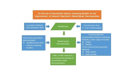
On the Use of Generalized Volume Scattering Models for the Improvement of General Polarimetric Model-Based Decomposition

Abstract

Recently, a general polarimetric model-based decomposition framework was proposed by Chen et al., which addresses several well-known limitations in previous decomposition methods and implements a simultaneous full-parameter inversion by using complete polarimetric information. However, it only employs four typical models to characterize the volume scattering component, which limits the parameter inversion performance. To overcome this issue, this paper presents two general polarimetric model-based decomposition methods by incorporating the generalized volume scattering model (GVSM) or simplified adaptive volume scattering model, (SAVSM) proposed by Antropov et al. and Huang et al., respectively, into the general decomposition framework proposed by Chen et al. By doing so, the final volume coherency matrix structure is selected from a wide range of volume scattering models within a continuous interval according to the data itself without adding unknowns. Moreover, the new approaches rely on one nonlinear optimization stage instead of four as in the previous method proposed by Chen et al. In addition, the parameter inversion procedure adopts the modified algorithm proposed by Xie et al. which leads to higher accuracy and more physically reliable output parameters. A number of Monte Carlo simulations of polarimetric synthetic aperture radar (PolSAR) data are carried out and show that the proposed method with GVSM yields an overall improvement in the final accuracy of estimated parameters and outperforms both the version using SAVSM and the original approach. In addition, C-band Radarsat-2 and L-band AIRSAR fully polarimetric images over the San Francisco region are also used for testing purposes. A detailed comparison and analysis of decomposition results over different land-cover types are conducted. According to this study, the use of general decomposition models leads to a more accurate quantitative retrieval of target parameters. However, there exists a trade-off between parameter accuracy and model complexity which constrains the physical validity of solutions and must be further investigated.

1. Introduction

Understanding of polarimetric scattering mechanisms is the bridge between the polarimetric synthetic aperture radar (PolSAR) measurements and both qualitative and quantitative retrieval of parameters describing physical processes on land cover [1]. According to the different ways an electromagnetic way can interact with vegetated and/or artificial targets it becomes necessary to have available mathematical and/or physical models which account for both geometrical and electromagnetic properties of matter. Polarimetric target decomposition techniques are designed to this aim. They can be devised to represent measured data either in terms of some polarimetric signature parameters (e.g. scattering entropy and mean scattering angle) or in a combination of some simple scattering mechanisms which describe first order scattering interactions [2]. Therefore, it is a widely employed tool to interpret scattering mechanisms present in the scene by exploiting PolSAR data. As known, polarimetric target decompositions are grouped into two main categories, i.e., Sinclair matrix-based coherent approaches and coherency/covariance matrix-based incoherent ones [2]. Eigenvalue-eigenvector-based and model-based methods are two major groups belonging to incoherent decompositions [1,2]. Two comprehensive reviews of this group of techniques can be found in [1,2]. The decomposition results have been used for a number of applications, such as target detection [3,4,5], land cover classification [6,7,8,9,10,11,12,13], and geophysical parameter inversion [14,15,16]. Freeman–Durden decomposition [17] is the pioneering work on model-based decompositions. Afterwards, many improved methods have been proposed to enhance the decomposition performance, such as Yamaguchi-based decomposition methods (e.g., Y4O [18], Y4R [19], S4R [20], and G4U [21]). Recently, a general decomposition method was proposed by Chen et al. [22], which exploits a variety of advances and key ideas in previous literature to deal with well-known limitations, such as model inversion priority, branch conditions, orientation effect and negative powers, and it utilizes the complete polarimetric information from the observed covariance/coherency matrix. The nine unknowns of the model can be retrieved simultaneously using a nonlinear least-squares optimization algorithm. Theoretically, it is one of the most complete and general approaches within the topic. In a recent contribution [23,24] we adopted this decomposition framework to check the feasibility of model-based decomposition output parameters from the perspective of quantitative applications. We proposed some modifications of the parameter inversion algorithm to obtain physically feasible parameter values. We will refer to this contribution hereafter as “modified parameter inversion algorithm” or “modified Chen method”.

However, as in the conclusions in both Chen’s original work [22] and Xie’s works [23,24], a future research direction is focused on the development or selection of more generalized volume scattering models rather than four specific types of volume scattering models. Usually, in order to characterize more complicated volume scattering in practice, the generalized volume scattering model will introduce one or even more new parameters. However, it should be noted that no additional observations are available. One way to overcome this limitation is by employing some strategy aimed at first predefining a potential candidate for the volume component on the basis of some physically-based assumption and according to the observed data themselves. Then, the remaining model parameters can be estimated. In this regard, this paper proposes the incorporation of both generalized volume scattering models proposed by Antropov et al. [25] and Huang et al. [26,27], named the generalized volume scattering model (GVSM) and simplified adaptive volume scattering model (SAVSM) respectively, into Chen’s decomposition framework. Moreover, in both approaches we adopt the improvements proposed in [23,24] for the retrieval algorithm in the optimization procedure. Besides, the two new algorithms reduce notably numerical issues and computation cost since they require only one nonlinear optimization instead of four as in Chen’s method.

The structure of this paper is organized as follows. In Section 2, Chen’s decomposition framework and modified parameters inversion algorithm from [19,20] are briefly reviewed. Then, both generalized volume scattering models by Antropov et al. and Huang et al. will be introduced. Afterwards, the two general decomposition methods and their corresponding decomposition procedures are proposed. Section 3 is divided into two main aspects. Firstly, it presents Monte Carlo simulation tests by using the modified Chen method and the proposed two algorithms using generalized volume scattering models. A comparative analysis of the inverted parameters is carried out to compare the performance of this three methods. Secondly, a fully polarimetric C-band Radarsat-2 image and a quad-polarization L-band AIRSAR image over the San Francisco area are used to compare the decomposition outputs of all three general decomposition methods together with the Yamaguchi decomposition with orientation compensation method (Y4R) [19]. A detailed analysis of the backscattering power component statistics over different land cover types is conducted. Finally, the major conclusions of this work are drawn in Section 4.

2. General Polarimetric Model-Based Decomposition

In this part, we briefly review the general decomposition framework proposed by Chen et al. [22], and the modified parameter inversion algorithm we proposed in [23,24]. Based on that, we proposed two general polarimetric model-based decomposition methods by using the generalized volume scattering model proposed either by Antropov et al. [25] or Huang et al. [26,27], respectively.

2.1. General Decomposition Framework

In [22], Chen et al. proposed a general polarimetric model-based decomposition method. It belongs to the family of four-component decomposition methods and can be expressed as:

$$T=f_v{T}_v+f_s{T}_s\left({\psi }_S\right)+f_d{T}_d\left({\psi }_D\right)+f_c{T}_c+T_{residual}$$

(1)

where $f_v$, $f_s$, $f_d$ and $f_c$ represent the coefficients of volume, surface, double-bounce and helix scattering, respectively. The volume scattering model included three traditional models, i.e., random, horizontal and vertical dipoles volume scattering models as in the Yamaguchi-based decomposition methods. Besides, it accounted for the entropy model [28], which does not have a clear physical meaning in terms of scene features but somehow relieves the overestimation of volume scattering power [25]. Moreover, considering that the terrain slopes and oriented building induce different cross-polarization scattering, it is conducted a polarimetric orientation compensation (also named deorientation processing) for odd- and double-bounce scattering models by rotating the coherency matrix with two independent orientation angles separately, i.e., ${\psi }_S$ and ${\psi }_D$. The helix scattering is roll-invariant and was originally proposed by Yamaguchi. In addition, the modeling error and observation noise were also considered as a residual term $T_{residual}$. The expressions of coherency matrix for different scattering components were given as

$$T_v^R=\frac{1}{4}\left[\begin{array}{ccc}2& 0& 0\\ 0& 1& 0\\ 0& 0& 1\end{array}\right]T_v^H=\frac{1}{30}\left[\begin{array}{ccc}15& 5& 0\\ 5& 7& 0\\ 0& 0& 8\end{array}\right]T_v^V=\frac{1}{30}\left[\begin{array}{ccc}15& -5& 0\\ -5& 7& 0\\ 0& 0& 8\end{array}\right]T_v^E=\frac{1}{3}\left[\begin{array}{ccc}1& 0& 0\\ 0& 1& 0\\ 0& 0& 1\end{array}\right]T_s=\left[\begin{array}{ccc}1& {\beta }^{*}& 0\\ \beta & {\left|\beta \right|}^2& 0\\ 0& 0& 0\end{array}\right]T_{\mathrm{d}}=\left[\begin{array}{ccc}{\left|\alpha \right|}^2& \alpha & 0\\ {\alpha }^{*}& 1& 0\\ 0& 0& 0\end{array}\right]$$

(2)

$$\begin{gathered} T_s\left({\psi }_S\right)=R_3\left({\psi }_S\right)T_s{R}_3^H\left({\psi }_S\right)T_d\left({\psi }_D\right)=R_3\left({\psi }_{\mathrm{D}}\right)T_{\mathrm{d}}{R}_3^H\left({\psi }_{\mathrm{D}}\right)\text{ where} \\ {R}_3\left(\psi \right)=\left[\begin{array}{ccc}1& 0& 0\\ 0& \cos 2\psi & \sin 2\psi \\ 0& -\sin 2\psi & \cos 2\psi \end{array}\right] \end{gathered}$$

(3)

For parameter inversion, all the nine independent real observations in the coherency matrix were considered. The unknown parameters were simultaneously and optimally solved by using the nonlinear least squares algorithm which minimized the sum of squares of the residual. The initial values of parameters were obtained from Yamaguchi-based methods and the boundaries conditions were set according to some physical constraints.

2.2. Modified Parameters Inversion Algorithm

Because the model parameter inversion is a nonlinear optimization problem, it sometimes will achieve a local minimum and produce non-physical solutions, which limits the quantitative application of measured polarimetric synthetic aperture radar (PolSAR) data with these model-based decomposition techniques. In order to address this issue, a quantitative examination of the accuracy of output parameters was carried out and a modified parameter inversion algorithm was proposed in [23,24]. The improvements concerned three aspects:

(1)

Redefining variable boundaries based on the physical constraints of dielectric constants and some implicit conditions of the model itself;

(2)

Generating the initial values accounting for physical constraints;

(3)

Implementing a transformation of variables to ease the selection of the upper and lower bounds required in the inversion algorithm.

For parameters inversion, a Matlab function named “lsqnonlin” with the trust-region-reflective algorithm is used in the nonlinear optimization. After these modifications, the results showed that the overall accuracy of parameter inversion was significantly improved [23,24].

2.3. Volume Scattering Model

In order to improve the aforementioned general decomposition framework for guaranteeing the parameters inversion as a determined problem and allowing for adjustment to the measured PolSAR data, the generalized volume scattering model (GVSM) proposed by Antropov et al. [25] and the simplified adaptive volume scattering model proposed (SAVSM) by Huang et al. [26,27] are adopted to construct two general model-based decomposition methods, respectively, which are described next.

2.3.1. Generalized Volume Scattering Model (GVSM)

The GVSM proposed by Antropov et al. is based on geophysical media symmetry properties, and has been shown to be more general than other traditional models for characterizing canopy scattering [25]. According to the expression of GVSM in the case of setting the value of shape parameter as 1/3 (i.e., dipoles) for the covariance matrix in [25], after using a unitary transformation, the corresponding coherency matrix can be derived as

$$T_v^{GVSM}\left(\gamma \right)=\frac{1}{\frac{3(1+\gamma )}{2}-\frac{\sqrt{\gamma }}{3}}\left[\begin{array}{ccc}\frac{1+\gamma }{2}+\frac{\sqrt{\gamma }}{3}& \frac{\gamma -1}{2}& 0\\ \frac{\gamma -1}{2}& \frac{1+\gamma }{2}-\frac{\sqrt{\gamma }}{3}& 0\\ 0& 0& \frac{1+\gamma }{2}-\frac{\sqrt{\gamma }}{3}\end{array}\right]$$

(4)

where $\gamma$ represents the co-polarization power ratio of HH and VV components, i.e., $\gamma =\langle {\left|S_{hh}\right|}^2\rangle /\langle {\left|S_{vv}\right|}^2\rangle$, which can be estimated directly from the measured PolSAR data. As was analyzed in [21], the GVSM model showed good agreement with the three typical cases of volume scattering model in Yamaguchi-based decomposition corresponding to three specific co-polarization power ratios (i.e., 8/3, 1, 3/8). However, besides these three cases, the GVSM can cover the whole dynamic range of values for the ratio. In order to further present the generality of GVSM, as proposed by Huang et al. [26,27], we employ two common scattering randomness measurements to analyze its dependence on the ratio $\gamma$. One is the radar vegetation index ($RVI$) introduced by Kim and van Zyl [29], which is an indicator to measure scattering randomness. The definition of $RVI$ is given as

$$RVI=\frac{4\min \left({\lambda }_1,{\lambda }_2,{\lambda }_3\right)}{{\lambda }_1+{\lambda }_2+{\lambda }_3}$$

(5)

where ${\lambda }_1$, ${\lambda }_2$, ${\lambda }_3$ are the eigenvalues of the covariance/coherency matrix. The values of $RVI$ range from 0 to 1. The other is the polarimetric scattering entropy $H$ proposed by Cloude and Pottier [6], which is also calculated from the eigenvalues and is defined as

$$H={\displaystyle \sum _{i=1}^N-P_i}{\log }_N{P}_i{P}_i=\frac{{\lambda }_i}{{\displaystyle {\sum }_{j=1}^N{\lambda }_i}}$$

(6)

where $N=3$ for the monostatic case. The value of $H$ is also limited between 0 and 1. The values of both two indices will monotonically rise with an increase of the degree of scattering randomness. Figure 1 shows the dependence of $RVI$ and $H$ on the ratio $\gamma$. It can be seen that the GVSM can consider more cases of scattering randomness inside the canopy, therefore, it can accommodate other different canopy morphologies without constraining the models to those commonly employed structures.

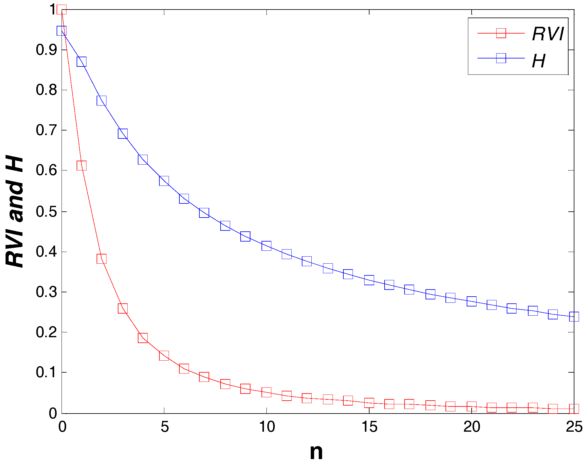
2.3.2. Simplified Adaptive Volume Scattering Model (SAVSM)

According to the basic idea to model the volume scattering in Freeman–Durden or Yamaguchi-based methods, the particles of the volume are assumed to be randomly distributed particles with one specific distribution. The simplified adaptive volume scattering model (SAVSM) proposed by Huang et al. [26,27] also followed this idea. It assumes that the volume is composed by randomly distributed thin cylinders (i.e., dipoles) and the orientation satisfies a n-power sine function (vertical orientation distribution) or cosine function (horizontal orientation distribution). After adopting the horizontal dipoles as the elemental particle and implementing the integration operation, the expressions of the coherency matrix of vertical SAVSM (V-SAVSM) and horizontal SAVSM (H-SAVSM) are given as [26,27]

$$T_V^{V-SAVSM}=\frac{1}{A}\left[\begin{array}{ccc}{T}_V^{11}& T_V^{12}& 0\\ T_V^{12}& T_V^{22}& 0\\ 0& 0& T_V^{33}\end{array}\right] T_V^{H-SAVSM}=\frac{1}{A}\left[\begin{array}{ccc}{T}_H^{11}& T_H^{12}& 0\\ T_H^{12}& T_H^{22}& 0\\ 0& 0& T_H^{33}\end{array}\right]$$

(7)

where

$$\begin{gathered} T_H^{11}=T_V^{11}=\frac{\sqrt{\pi }\mathsf{\Gamma }\left(\frac{n+1}{2}\right)}{2\mathsf{\Gamma }\left(\frac{n}{2}+1\right)},T_H^{12}=-T_V^{12}=\frac{n\sqrt{\pi }\mathsf{\Gamma }\left(\frac{n+1}{2}\right)}{4\mathsf{\Gamma }\left(\frac{n}{2}+2\right)} \\ {T}_H^{22}=T_V^{22}=\frac{\left(n^2+2n+4\right)\sqrt{\pi }\mathsf{\Gamma }\left(\frac{n+1}{2}\right)}{8\mathsf{\Gamma }\left(\frac{n}{2}+3\right)} \\ {T}_H^{33}=T_V^{33}=\frac{\sqrt{\pi }\mathsf{\Gamma }\left(\frac{n+3}{2}\right)}{\mathsf{\Gamma }\left(\frac{n}{2}+3\right)} \\ A={\displaystyle {\int }_0^{\pi }{\sin }^n\theta }d\theta ={\displaystyle {\int }_{-\frac{\pi }{2}}^{\frac{\pi }{2}}{\cos }^n\theta }d\theta =\frac{\sqrt{\pi }\mathsf{\Gamma }\left(\frac{n+1}{2}\right)}{\mathsf{\Gamma }\left(\frac{n}{2}+1\right)} \\ \mathsf{\Gamma }\left(x\right)={\displaystyle {\int }_0^{\infty }{e}^{-t}}{t}^{x-1}dt \end{gathered}$$

(8)

From the above expressions, it can be seen that the SAVSM includes two categories and depends on the power variable $n$, which is a real value. Actually, it is not difficult to check that the three volume scattering models in Yamaguchi decomposition method are exactly three special cases in SAVSM. In addition, when $n=0$, it satisfies $T_V^{H-SAVSM}=T_V^{V-SAVSM}$. However, the SAVSM covers more types of volume scattering model aside from these three cases. Because the SAVSM includes two categories, the first step should be selecting one of them according to a certain criterion. As in the Yamaguchi decomposition method [18,19,20,21], the co-polarization power ratio $\gamma$ (i.e., $\gamma =\langle {\left|S_{hh}\right|}^2\rangle /\langle {\left|S_{vv}\right|}^2\rangle$) is used to determine the type of volume scattering model. The volume scattering model will choose the random dipoles volume scattering model when $\gamma$ is within $\pm 2dB$, whereas it will select horizontal dipoles model for $\gamma >2dB$ and vertical dipoles model for $\gamma <-2dB$. Figure 2 shows the dependence of co-polarization power ratios of H-SAVSM and V-SAVSM on the power variable n. From this figure, it is evident that a null ratio is a suitable threshold to distinguish the H-SAVSM and V-SAVSM, which is not the same criterion used by Huang et al. [27]. Afterwards, the next step should be determining the value of $n$. Since $n$ is used to define the probability density function of the orientation of particles, its value will determine the degree of scattering randomness. As shown in [26,27], the dependence of the common scattering randomness measurements $RVI$ and $H$ on the value of $n$ is illustrated in Figure 3. It is obvious that the values of both parameters decrease monotonically when $n$ increases from zero to infinity. As in Huang et al. [27], based on the relationship between $RVI$ and $n$, the optimum n can be determined when the difference between the $RVI$ of covariance/coherency matrix and the $RVI$ of SAVSM is minimum. The criterion is described as

$$\min \left|RV{I}_{C/T}-RV{I}_{SAVSM}\left(n\right)\right|$$

(9)

From Figure 3, it can be observed that the value of $RVI$ is almost unchanged when $n$ arrives at 20. Therefore, the maximum $n$ is limited at 20 as used by Huang et al. [26].

2.4. The Proposed Modified Algorihtms

Based on the aforementioned discussion and the general decomposition framework by Chen et al. [22], and GVSM [25] and SAVSM [26,27] models, we propose two modified algorithms of model-based decomposition. The general expression of decomposition models for both methods in the Pauli basis (i.e., coherency matrix) is given as

$$T=f_v{T}_v^G+f_s{T}_s\left({\psi }_S\right)+f_d{T}_d\left({\psi }_D\right)+f_c{T}_c+T_{residual}$$

(10)

where $T_v^G$ represents the generalized volume scattering model, which can be either GVSM or SAVSM. It must be noted that the elements of $T_v^G$ in both cases will be determined externally before parameter inversion. The detailed processing steps of both decomposition methods are presented next.

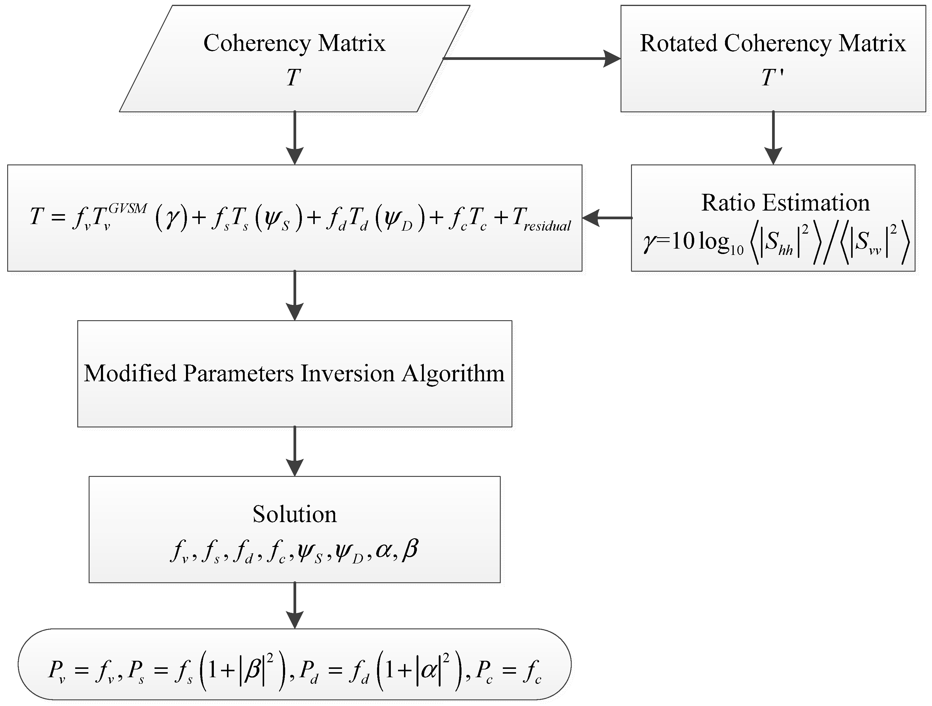
2.4.1. General Polarimetric Model-Based Decomposition with GVSM

After substituting the GVSM, the general decomposition model in coherency matrix form can be expressed as

$$T=f_v{T}_v^{GVSM}\left(\gamma \right)+f_s{T}_s\left({\psi }_S\right)+f_d{T}_d\left({\psi }_D\right)+f_c{T}_c+T_{residual}$$

(11)

The ratio $\gamma$ is directly estimated according to the measured coherency matrix. As this parameter $\gamma$ describes the elements of the volume matrix components, we first apply Lee’s polarimetric orientation compensation [30] in order to lower the coupling to the volume component of other scattering sources not originated within the canopy. For every pixel, as $\gamma$ is computed, the corresponding volume model will be determined according to Equation (4), hence no new unknowns are added to the inversion step. Afterwards, the nine-unknown equation system will be solved by using a nonlinear least-square optimization based on the modified parameters inversion algorithm as proposed in [23,24]. The flowchart of this method is shown in Figure 4.

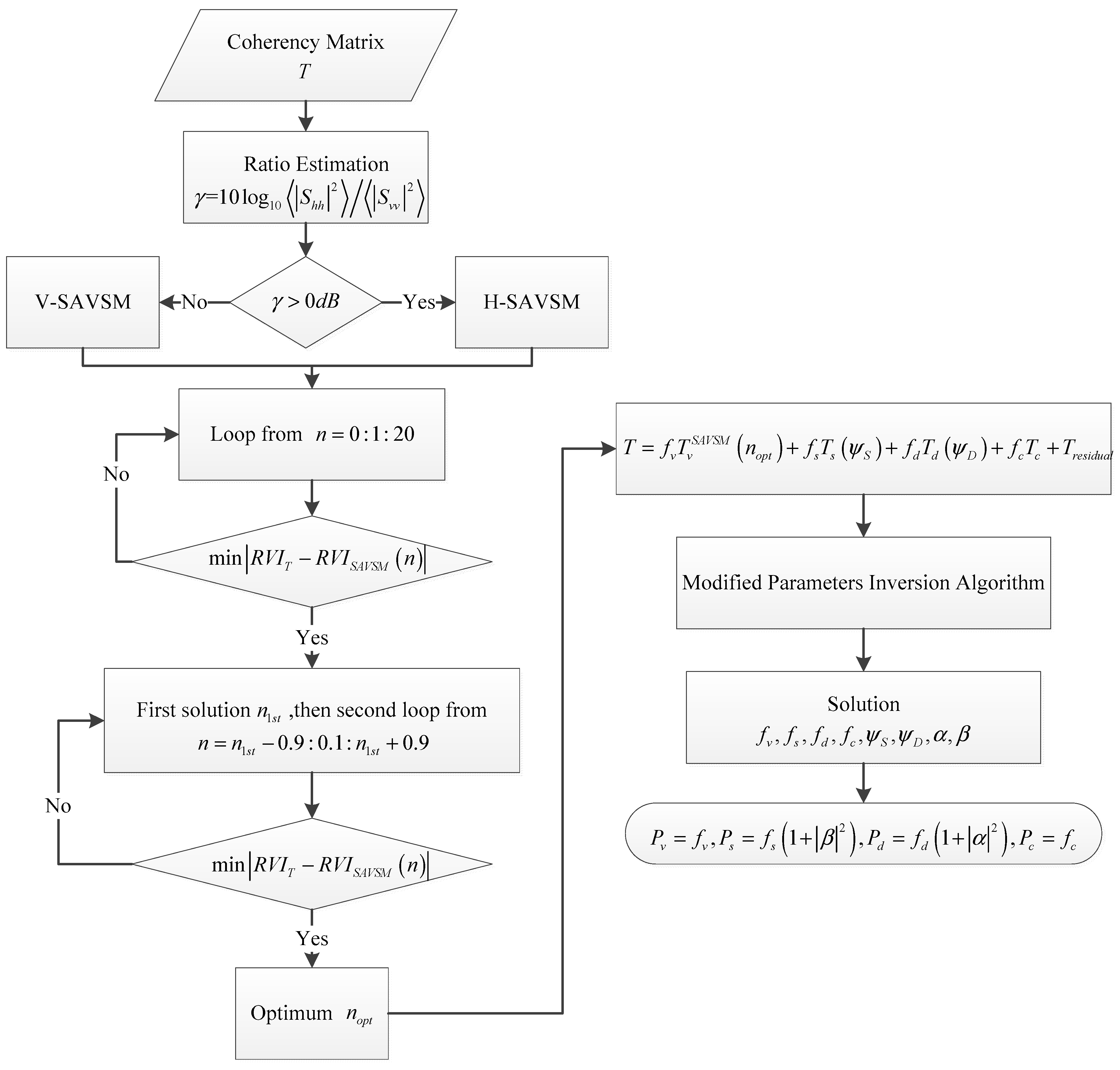
2.4.2. General Polarimetric Model-Based Decomposition with SAVSM

In a similar way, after incorporating SAVSM, the general decomposition model in the Pauli basis is expressed as

$$T=f_v{T}_v^{SAVSM}\left(n\right)+f_s{T}_s\left({\psi }_S\right)+f_d{T}_d\left({\psi }_D\right)+f_c{T}_c+T_{residual}$$

(12)

As described in Section 2.3.2, the first stage computes the ratio $\gamma$ to determine whether the volume model belongs to the horizontal or vertical SAVSM family. The second step is to obtain the optimum n by comparing the difference of RVI as seen in Equation (9). As mentioned before, $n$ is real and has been limited to be less than 20. Therefore, the number of available candidates of n and, consequently, the computation cost of this stage depends on the sampling interval of $n$. In this paper, we choose 0.1 as the sampling interval of $n$, because the dependence on $n$ in Figure 2 and Figure 3 is very smooth. Moreover, in order to further improve the computation efficiency, we propose a “two-step” algorithm to determine $n$ rather than directly divide the range of $n$ by using the interval of 0.1. The first step is using a coarse grid (step equal to 1) to obtain the initial guess of $n$. Then the second step is adopting the narrow step of 0.1 to construct the searching space according to the value of $n$ derived from the first step. After that, the optimum $n$ is obtained and then the corresponding SAVSM is also determined. Later, the solution of nine unknowns will be obtained by using a nonlinear least-square optimization based on the modified parameters inversion algorithm as proposed in [23,24]. Figure 5 presents the flowchart of the whole procedure of this algorithm.

3. Results

In practice, it is well-known the existing difficulty to evaluate the decomposition performance in a real situation because of the lack of ground truth. Therefore, the alternative way to address this issue is to use simulations. Afterwards, both L- and C-band satellite image were also used and a comparison of results derived from different decomposition methods was conducted.

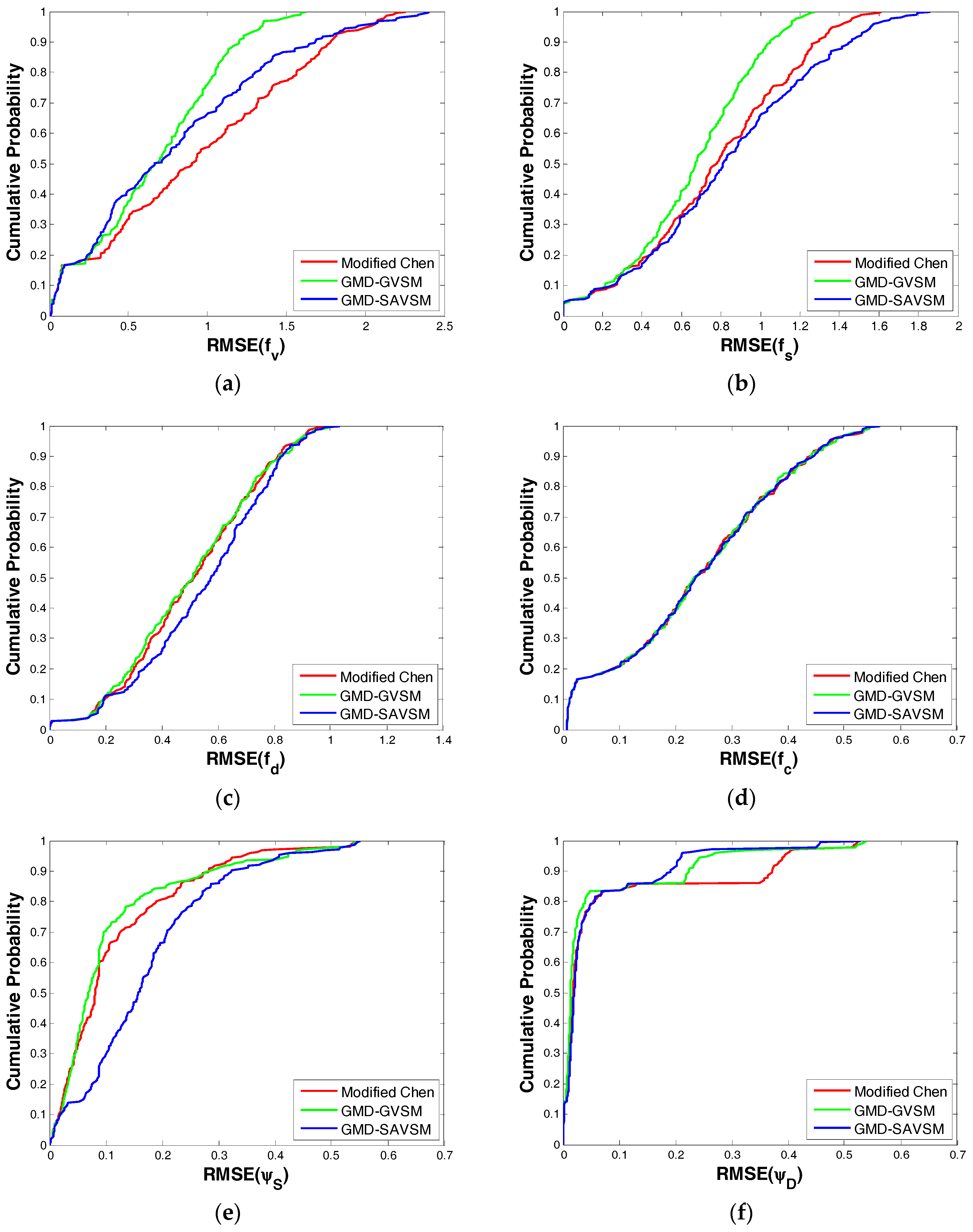
3.1. Monte Carlo Simulations

In our simulations, we followed the classical Monte Carlo simulation method for PolSAR data proposed by Lee [31]. As shown in

Table 1. Values for input parameters.

Parameter	Quantity	Value
$f_v$	volume scattering coefficient	0:2:10
$f_s$	surface scattering coefficient	0:2:10
$f_d$	dihedral scattering coefficient	0:2:10
$f_c$	helix scattering coefficient	0.01
${\psi }_s$	orientation angle in surface scattering model	−10°
${\psi }_d$	orientation angle in dihedral scattering model	−15°
$\alpha$	ratio parameter in dihedral scattering model	0.3515–0.0768i
$\beta$	ratio parameter in surface scattering model	−0.3377
$\theta$	incidence angle	45°
$\varphi$	differential propagation phase	10°
${\epsilon }_s$	soil dielectric constant	10
${\epsilon }_t$	trunk dielectric constant	30

, in order to simulate a wide variety of cases, we employed a large enough interval of values to specify the volume, surface, and dihedral scattering coefficients. The uniformly oriented random dipoles volume model was selected in simulations. By doing so, according to Equation (1), we simulated 216 different cases by varying $f_v$, $f_s$ and $f_d$ (six values per parameter). Therefore, a wide variety of scattering scenarios is considered, i.e., one dominant mechanism out of three (helix scattering is assumed to be fixed and very low) or other mixed cases with no dominant mechanism. In every case, we performed 1000 realizations and 15 × 15 looks were averaged for reducing speckle noise.

For every case, we tested three general model-based decomposition (GMD) methods: (1) “Modified Chen”: This is assumed as the reference method, i.e., the original model proposed in [22] with the modified parameter inversion algorithm in [23,24]; (2) “GMD–GVSM”: The first proposed method, i.e., incorporating the GVSM in [25] also with the modified parameter inversion algorithm in [23,24]; (3) “GMD–SAVSM”: The second proposed method, i.e., incorporating the SAVSM in [26,27] also with the modified parameter inversion algorithm in [23,24]. In order to quantitatively assess the respective performances, we firstly calculated the root mean square error (RMSE) for every model parameter according to 1000 realizations. Then, as shown in Figure 6, we computed the corresponding cumulative probability distribution curves of RMSE of all parameters for all the 216 different cases. Note that the cumulative distribution function is defined as

$$F_X\left(x\right)=P\left(X\le x\right)$$

(13)

where the function value represents the probability that the random variable $X$ chooses a value less than or equal to x. Since x here is represented by RMSE, it means that the accuracy of the retrieved parameter is higher when the curve reaches saturation faster.

Figure 6 shows cumulative probability distribution curves of RMSE of all nine model parameters obtained from the three general decomposition methods. From this figure, some comments are in order:

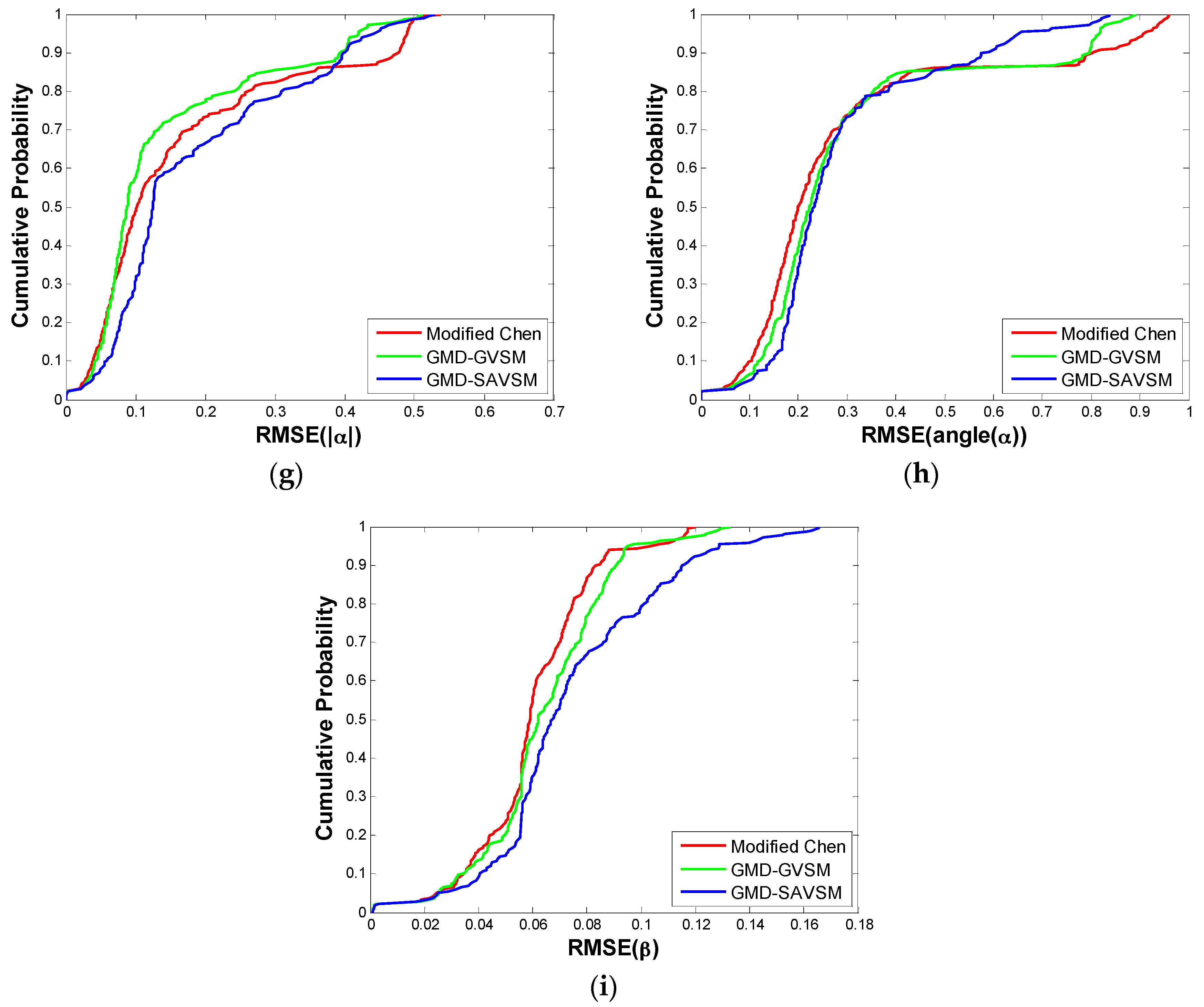
• For the four backscattering coefficients, the results of $f_v$ and $f_s$ from the “GMD–GVSM” method show significant improvements compared with the “Modified Chen” method, whereas the result of $f_d$ exhibits only a slight improvement. The “GMD–SAVSM” method also shows a slightly higher accuracy in the volume scattering coefficient $f_v$, however, it produces slightly poorer performance in $f_s$ and $f_d$. The results of $f_c$ from all three methods are very similar.
• For the two orientation angle parameters, the “GMD–GVSM” method also produces some improvement. Moreover, the accuracy of the double-bounce orientation angle ${\psi }_D$ is higher than the surface orientation angle ${\psi }_S$ reaching a high probability of 0.8 with lower RMSE. Similarly, the “GMD–SAVSM” method also shows better performance in the double-bounce orientation angle and its accuracy is better than the surface orientation angle. However, for the inversion of surface orientation angle, the “GMD–SAVSM” has not shown improvement compared with the “Modified Chen” method.
• For the two ratio parameters, the “GMD–GVSM” method shows some improvement in the absolute value of alpha, while performance slightly degrades for the phase of alpha. Although the result of beta from the “GMD–GVSM” method is slightly worse than from the original method, it is noted that it is still a reasonable estimate since the probability of success in the retrieval is 80% allowing a 0.08 RMSE value. However, the performance of “GMD–SAVSM” is clearly poorer in all ratio parameters in comparison with the other two methods.

3.2. Real Data Test

In this section, we provide two examples to demonstrate and compare the decomposition performances from different methods. In addition to the “Modified Chen” method and the two proposed general decomposition methods, i.e., ”GMD–GVSM” and “GMD–SAVSM”, one traditional four-component decomposition method, i.e., Yamaguchi decomposition with orientation compensation (Y4R [19]) was also tested as a benchmark method. Two collected experimental datasets both cover San Francisco, CA, USA (Lat/Lon, N37.78°/W122.48°), which is useful for comparative analysis. One is C-band quad-polarization fine-beam-mode (FQ9) Radarsat-2 satellite data acquired on 9 April 2008, and the other is L-band AIRSAR airborne multi-look complex (MLC) PolSAR data acquired on 11 May 1999. A detailed analysis of the results for each data is presented next.

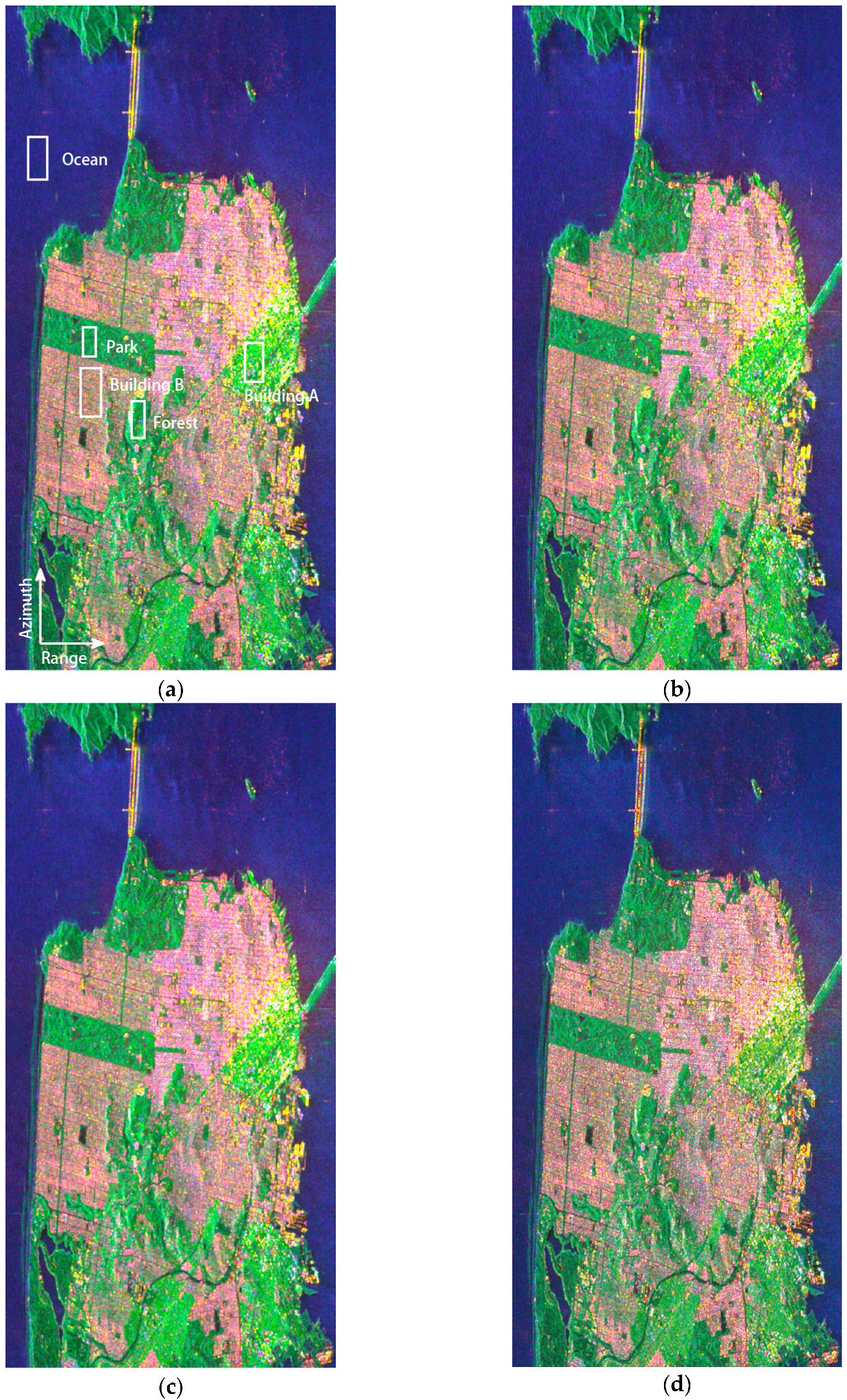
3.2.1. Radarsat-2 Satellite Data

In the preprocessing step, a 7 × 7 boxcar filter was applied to reduce the speckle noise and then the corresponding coherency matrix was estimated. A portion of the whole image with a size of 2990 × 1440 pixels was selected in the test, in which ocean, park, built-up and forest areas were included. The resolution in azimuth and range direction is 4.8 m and 4.7 m, respectively. The corresponding incidence angle range is narrow varying from 28.45° to 29.38°.

The decomposition results from these four methods are shown in Figure 7. From the visual perspective of this figure, all the results are similar. As expected, the color in forest and park areas, where volume scattering is dominant, is green, and the ocean areas, where surface scattering is dominant, is blue. For the build-up areas, the color is red in general because double-bounce scattering is dominant. However, in largely oriented build-up areas, such as the triangle area located in the right-middle of Figure 7 (denoted as building A), the color is mostly green. It means the volume scattering component is still overestimated in these areas despite the orientation compensation has been considered in these four methods, and consequently, this issue requires further investigation.

To compare the decomposition performances in detail, five types of land cover classes are considered in the image: forest area, park area, largely oriented build-up area (Build-up A), slightly oriented build-up area (Build-up B), and ocean area. The boundaries of these areas of interest are marked in white in Figure 7a. Note that it is still a difficult issue to verify which decomposition method is most consistent with the ground truth. Therefore, we just compare the decomposition performances and provide some possible physical explanations.

Table 2. Statistics of power of scattering components of Radarsat2 image in selected areas with different land cover classes.

Area	Methods	Ps(%)	Pd(%)	Pv(%)	Pc(%)
Forest	Y4R	35.98	13.72	45.21	5.09
	Modified Chen	34.71	22.48	37.73	5.08
	GMD–GVSM	32.48	21.02	41.40	5.10
	GMD–SAVSM	33.81	21.76	39.30	5.12
Park	Y4R	29.31	11.51	53.21	5.97
	Modified Chen	29.88	20.09	44.06	5.97
	GMD–GVSM	26.47	18.75	48.79	5.99
	GMD–SAVSM	28.77	19.80	45.40	6.03
Build-up A	Y4R	20.51	35.34	37.53	6.62
	Modified Chen	20.10	40.57	32.74	6.59
	GMD–GVSM	19.73	40.95	32.66	6.66
	GMD–SAVSM	20.31	42.04	30.94	6.71
Build-up B	Y4R	33.48	48.35	14.15	4.01
	Modified Chen	25.27	56.83	13.89	4.00
	GMD–GVSM	26.54	55.15	14.29	4.01
	GMD–SAVSM	27.75	53.53	14.68	4.04
Ocean	Y4R	95.12	1.86	2.60	0.41
	Modified Chen	93.39	4.52	1.68	0.41
	GMD–GVSM	93.33	4.52	1.74	0.41
	GMD–SAVSM	93.01	4.43	2.15	0.41

shows the results of scattering power component contribution statistics from the different methods in these areas. In the forest area, all three methods show the volume scattering is dominant. Compared with Y4R, the results from both the “Modified Chen” and two proposed methods somehow reduce the volume scattering component and increase the double-bounce scattering component. The forest area we selected is a part of Mount Sutro forest from which about 80% is made up of eucalyptus trees, which exhibit a large trunk but a low density crown. This kind of structure eases the radar wave to penetrate through the crown and to reach the ground. Hence, double-bounce scattering from ground-trunk structure is expected to appear. Among all four methods, the modified Chen method estimates the lowest value for the volume component. The reason is that about 40% of pixels in this box choose the entropy model as the volume scattering model, which as expected provides a much lower estimate of volume scattering component since $P_v$ reaches a value of $6\langle {\left|S_{hv}\right|}^2\rangle$ at most. In the park area, the dominant scattering component at all methods is consistently the volume scattering. The “Modified Chen” and the two proposed methods yield a higher double-bounce scattering, which could be attributed to the building targets inside the park. In the highly oriented build-up area A, the “Modified Chen” and the two proposed methods retrieve a higher percentage of double-bounce scattering component and a lower one of volume scattering component in comparison to Y4R method. A similar behavior is obtained in the slightly oriented build-up area B. In the ocean area, all methods consistently show a very high surface scattering, which is attributed to the water body being illuminated at C-band.

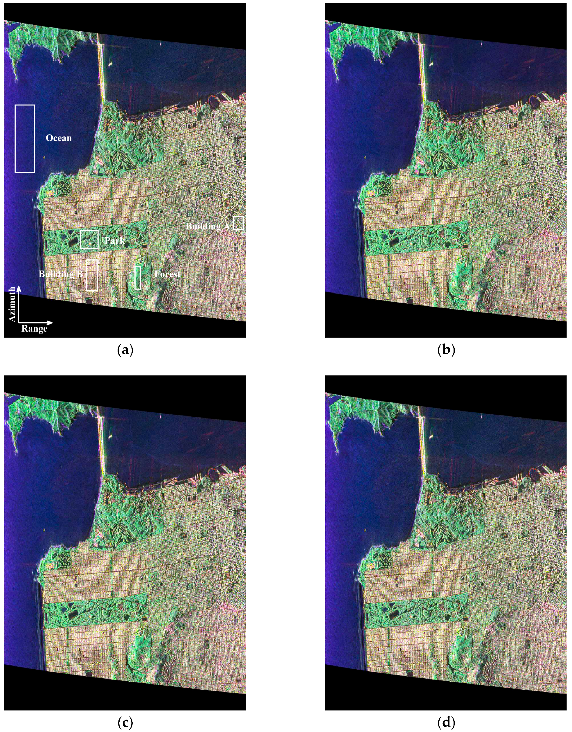
3.2.2. AIRSAR Airborne Data

The nominal pixel spacing parameters for original L-band AIRSAR MLC full polarimetric data in azimuth and range directions are 9.26 m and 3.3 m, respectively. As usual, a multi-look processing with 3 azimuth looks was applied for obtaining better visual presentation with near-squared pixels and further speckle reduction. Simultaneously, the corresponding coherency matrix was generated. Finally, the size of whole image in azimuth and range directions for decomposition is 1168 × 843. The incidence angle highly varies from 28.40° to 62.68°.

Figure 8 shows the decomposition results from these four methods. According to a visual inspection, no evident differences can be seen in all four results. In forest and park areas, the volume scattering power is relatively dominant in most pixels (green color). The ocean areas present dominant surface scattering, hence the color is blue. For the build-up areas, the volume scattering component is still overestimated specially in those largely oriented build-up areas in patch A.

As in the case of C-band data, we also provide the statistics of powers from different scattering components (see

Table 3. Statistics of power of scattering components in selected areas of L-band AIRSAR image with different land cover classes.

Area	Methods	Ps(%)	Pd(%)	Pv(%)	Pc(%)
Forest	Y4R	27.81	18.59	44.92	8.68
	Modified Chen	27.36	29.30	34.66	8.68
	GMD–GVSM	26.20	28.67	36.43	8.70
	GMD–SAVSM	26.17	28.55	36.57	8.71
Park	Y4R	29.43	29.20	34.71	6.66
	Modified Chen	24.93	40.21	28.21	6.65
	GMD–GVSM	24.67	39.50	29.16	6.67
	GMD–SAVSM	25.15	37.83	30.34	6.68
Build-up A	Y4R	30.99	37.60	24.74	6.67
	Modified Chen	27.22	49.62	16.59	6.57
	GMD–GVSM	27.34	49.11	16.96	6.59
	GMD–SAVSM	26.03	47.18	20.20	6.59
Build-up B	Y4R	21.41	59.42	16.10	3.07
	Modified Chen	15.53	68.22	13.19	3.06
	GMD–GVSM	16.25	66.32	14.37	3.06
	GMD–SAVSM	16.18	62.05	18.70	3.07
Ocean	Y4R	93.85	1.86	3.52	0.77
	Modified Chen	91.82	5.35	2.06	0.77
	GMD–GVSM	91.71	5.31	2.21	0.77
	GMD–SAVSM	91.18	5.31	2.75	0.76

) over five test areas including forest area, park area, largely oriented build-up area (Build-up A), slightly oriented build-up area (Build-up B), and ocean area. As shown in Figure 8a, the boundaries of these areas of interest are selected in similar regions as in the Radarsat2 image shown in Figure 7a. From Table 3, we can make the following comments. In the forest area, a similar trend is observed as in the results from C-band data. The volume scattering in forest area is consistently dominant in four methods. The Y4R method is outperformed by the other three general methods since they present a lower volume scattering component and a higher double-bounce scattering mechanism. The modified Chen method presents the lowest volume scattering component. In this case about 27% of pixels select the entropy volume scattering model. In the park area, a different scattering interpretation between different frequencies can be retrieved. The dominant scattering component from Y4R method is still the volume scattering. However, the “Modified Chen” and the two proposed methods show dominant double-bounce scattering rather than volume scattering as happened in case of C-band data. One explanation is that higher penetration at longer radar wavelength results in an enhanced double-bounce scattering within the building targets inside the park. In the highly oriented build-up area A, the compensation of orientation performs much better at L-band than at C-band, as expected. According to the volume backscattering powers their values are clearly reduced at L-band and similar to those obtained for the built-up B area. On the contrary, this volume scattering compensation is only marginally achieved at C-band, even though the three general methods still outperform Y4R. In the ocean area, as expected, all methods consistently show a very high surface scattering as in C-band case.

4. Discussion

4.1. Contribution to PolSAR Target Decomposition Methologies

The general decomposition framework we adopt is the one proposed by Chen et al. [22], which involves a number of advances and key ideas in this topic and has demonstrated some advances in scattering mechanism interpretation. In order to further improve the physical reliability of decomposition results derived from this method, the related parameter inversion algorithm should be an active research line. In this regard, the work contributed by Xie et al. [23,24] is intended to fill this gap. Another complementary direction is carrying out research from the perspective of the employed scattering models, especially the ones regarding volume scattering component since it has been extensively shown in the literature as a challenging task in radar remote sensing. The present work is intended to contribute in this direction. Therefore, this paper makes use of two general decomposition models to investigate how they can contribute to improve the retrieval performance of target decomposition methods. From the extensive simulation tests, it can be suggested that compared with the reference method, i.e., “Modified Chen” approach, the “GMD–GVSM” method shows overall improvements in the derived decomposition results as expected, even though the differences seem to be not so critical. According to these simulations, the generalized volume scattering model (GVSM) proposed by Antropov et al. is efficiently coupled with Chen’s decomposition framework to improve the reliability of decomposition results. However, the “GMD–SAVSM” method just showed some improvement in the volume scattering coefficient $f_v$ and double-bounce orientation angle ${\psi }_D$ and is clearly outperformed by “GMD–GVSM” and the “Modified Chen” approaches. The possible reasons for the poorer results in “GMD–SAVSM” may be due to the use of $RVI$ as the index for defining the volume model and/or that the interval 0.1 employed to determine $n$ is not enough to obtain an accurate approximation of the volume scattering model. Nevertheless, this issue requires further investigation. From the perspective of computation efficiency, the two proposed methods need just one time-consuming non-linear optimization calculation to retrieve model parameters instead of four as in Chen’s method. Moreover, the “GMD–SAVSM” method needs two simple loops to determine optimum $n$, whereas the “GMD–GVSM” only requires the calculation of a ratio. Therefore, one practical contribution of this work is that the proposed “GMD–GVSM” method is a promising methodology for quantitative target decompositions.

4.2. Radar Frequency Issue

In this study, we present decomposition results at C- and L-band over same test site. From the results, the scattering interpretation results from model-based decomposition at two frequencies present some differences. For example, the park area at L-band shows dominant double-bounce scattering, whereas it presents dominant volume scattering at C-band, according to the three general methods. However, the traditional Y4R method do not detect this difference. Another aspect is the problem of overestimating volume scattering in highly oriented built-up areas can be mitigated to some extent depending on the sensor frequency. This is clearly visible when comparing urban areas A, whose pattern is oblique with respect to the flight path, and B, whose street alignment is parallel/perpendicular to it. At L-band, both the Modified Chen and GMD–GVSM method reach a substantial reduction of the volume scattering their values being similar to those obtained for the B area. Nevertheless, this volume scattering compensation is only marginally achieved at C-band, even though the three general methods still outperform Y4R. As expected, the polarimetric response of the same target may differ at different frequencies, hence, some caution must be taken when interpreting scattering mechanisms according to model-based decomposition results in order to avoid ambiguities. These qualitative observations have been also confirmed in other recent publications [32].

4.3. Future Research Directions

Future work should be mainly focused on five aspects. First, the four typical volume scattering models and the two generalized volume scattering models tested in this paper all assume the particles of the volume are thin cylinders and reflection symmetry. Therefore, in the future more representative volume scattering models should be included and/or developed to improve the correspondence with the scene features and, consequently, the decomposition performance. Second, the ideas discussed in this study can be exported to the PolInSAR decomposition framework, and then the number of independent observations will increase significantly. Therefore, more complicated generalized volume scattering models with more parameters could be considered. Moreover, all the parameters can be directly solved without determining the volume scattering model previously or according to an iteration inversion scheme. Third, since the parameters inversion is a nonlinear optimization problem, exploiting ways to avoid sticking in local minima by “smoothing” objective functions is also considered as a future research. Fourth, testing and analyzing decomposition performance at different radar frequencies also need further investigation. Finally, the design of experiments leading to further investigate the reliability of this group of PolSAR techniques from the quantitative perspective is still a pending task.

5. Conclusions

The utility of generalized volume scattering model to general model-based decomposition is investigated in this paper. To do so, we make use of two general polarimetric model-based decomposition methods, i.e., “GMD–GVSM” and “GMD–SAVSM” methods. Based on the general decomposition framework recently proposed by Chen et al., either the generalized volume scattering model by Antropov et al. or Huang et al. are incorporated, respectively. Hence, those methods provide a wide range of volume scattering models rather than just four typical volume scattering models. The expressions of these two generalized volume models for every pixel are directly estimated by the observed data themselves according to different algorithms, hence they do not increase the number of unknowns to keep the parameter inversion as a determined problem. Moreover, they just need one non-linear optimization calculation to retrieve model parameters instead of four as in Chen’s method. Therefore, they can significantly reduce both numerical issues and the computation cost. Besides, the methodology presented in this paper adopts the modified parameter inversion algorithm we proposed in a previous work which is based on Chen’s approach and, consequently, a higher estimation accuracy and physically reliable parameter values are obtained. A number of Monte Carlo simulations are performed for testing purposes. Results have shown that the proposed “GMD–GVSM” method outperforms the “GMD–SAVSM” method and the previous existing strategies for PolSAR model-based parameter inversion. Analyses of a Radarsat-2 C-band image and an AIRSAR L-band image have also revealed quantitative differences among the four methodologies at these two radar frequencies that have been assessed. As an overall conclusion we can state that the “GMD–GVSM” method is a promising methodology for quantitative target decompositions.

References

1. Chen, S.W.; Li, Y.Z.; Wang, X.S.; Xiao, S.P.; Sato, M. Modeling and interpretation of scattering mechanisms in polarimetric synthetic aperture radar: Advances and perspectives. IEEE Signal Process. Mag. 2014, 31, 79–89. [Google Scholar] [CrossRef]
2. Cloude, S.R.; Pottier, E. A review of target decomposition theorems in radar polarimetry. IEEE Trans. Geosci. Remote Sens. 1996, 34, 498–518. [Google Scholar] [CrossRef]
3. Wang, W.; Ji, Y.; Lin, X. A novel fusion-based ship detection method from Pol-SAR images. Sensors 2015, 15, 25072–25089. [Google Scholar] [CrossRef] [PubMed]
4. Xiang, D.; Tang, T.; Hu, C.; Fan, Q.; Su, Y. Built-up area extraction from PolSAR imagery with model-based decomposition and polarimetric coherence. Remote Sens. 2016, 8. [Google Scholar] [CrossRef]
5. Shibayama, T.; Yamaguchi, Y.; Yamada, H. Polarimetric scattering properties of landslides in forested areas and the dependence on the local incidence angle. Remote Sens. 2015, 7, 15424–15442. [Google Scholar] [CrossRef]
6. Cloude, S.R.; Pottier, E. An entropy based classification scheme for land applications of polarimetric SAR. IEEE Trans. Geosci. Remote Sens. 1997, 35, 68–78. [Google Scholar] [CrossRef]
7. Lee, J.S.; Grunes, M.R.; Ainsworth, T.L.; Du, L.J.; Schuler, D.L.; Cloude, S.R. Unsupervised classification using polarimetric decomposition and the complex Wishart classifier. IEEE Trans. Geosci. Remote Sens. 1999, 37, 2249–2258. [Google Scholar]
8. Famil, L.F.; Pottier, E.; Lee, J.S. Unsupervised classification of multifrequency and fully polarimetric SAR images based on the H/A/Alpha-Wishart classifier. IEEE Trans. Geosci. Remote Sens. 2001, 39, 2332–2342. [Google Scholar] [CrossRef]
9. Shimoni, M.; Borghys, D.; Heremans, R.; Perneel, C.; Acheroy, M. Fusion of PolSAR and PolInSAR data for land cover classification. Int. J. Appl. Earth Obs. Geoinf. 2009, 11, 169–180. [Google Scholar] [CrossRef]
10. Qi, Z.; Yeh, A.G.; Li, X.; Lin, Z. A novel algorithm for land use and land cover classification using RADARSAT-2 polarimetric SAR data. Remote Sens. Environ. 2012, 118, 21–39. [Google Scholar] [CrossRef]
11. Antropov, O.; Rauste, Y.; Astola, H.; Praks, J.; Hame, T.; Hallikainen, M.T. Land cover and soil type mapping from spaceborne polsar data at l-band with probabilistic neural network. IEEE Trans. Geosci. Remote Sens. 2014, 52, 5256–5270. [Google Scholar] [CrossRef]
12. Hong, S.H.; Kim, H.O.; Wdowinski, S.; Feliciano, E. Evaluation of polarimetric SAR decomposition for classifying wetland vegetation types. Remote Sens. 2015, 7, 8563–8585. [Google Scholar] [CrossRef]
13. Zhang, X.; Dierking, W.; Zhang, J.; Meng, J. A polarimetric decomposition method for ice in the bohai sea using C-band PolSAR data. IEEE J. Sel. Top. Appl. Earth Obs. Remote Sens. 2015, 8, 47–66. [Google Scholar] [CrossRef]
14. Hajnsek, I.; Pottier, E.; Cloude, S.R. Inversion of surface parameters from polarimetric SAR. IEEE Trans. Geosci. Remote Sens. 2003, 41, 727–744. [Google Scholar] [CrossRef]
15. Hajnsek, I.; Jagdhuber, T.; Schon, H.; Papathanassiou, K.P. Potential of estimating soil moisture under vgetation cover by means of PolSAR. IEEE Trans. Geosci. Remote Sens. 2009, 47, 442–454. [Google Scholar] [CrossRef]
16. Jagdhuber, T.; Hajnsek, I.; Papathanassiou, K.P. An iterative generalized hybrid decomposition for soil moisture retrieval under vegetation cover using fully polarimetric SAR. IEEE J. Sel. Top. Appl. Earth Obs. Remote Sens. 2015, 8, 3911–3922. [Google Scholar] [CrossRef]
17. Freeman, A.; Durden, S.L. A three-component scattering model for polarimetric SAR data. IEEE Trans. Geosci. Remote Sens. 1998, 36, 963–973. [Google Scholar] [CrossRef]
18. Yamaguchi, Y.; Moriyama, T.; Ishido, M.; Yamada, H. Four-component scattering model for polarimetric SAR image decomposition. IEEE Trans. Geosci. Remote Sens. 2005, 43, 1699–1706. [Google Scholar] [CrossRef]
19. Yamaguchi, Y.; Sato, A.; Boerner, W.M.; Sato, R.; Yamada, H. Four-component scattering power decomposition with rotation of coherency matrix. IEEE Trans. Geosci. Remote Sens. 2011, 49, 2251–2258. [Google Scholar] [CrossRef]
20. Sato, A.; Yamaguchi, Y.; Singh, G.; Park, S.E. Four-component scattering power decomposition with extended volume scattering model. IEEE Geosci. Remote Sens. Lett. 2012, 9, 166–170. [Google Scholar] [CrossRef]
21. Singh, G.; Yamaguchi, Y.; Park, S.E. General four-component scattering power decomposition with unitary transformation of coherency matrix. IEEE Trans. Geosci. Remote Sens. 2013, 51, 3014–3022. [Google Scholar] [CrossRef]
22. Chen, S.W.; Wang, X.S.; Xiao, S.P.; Sato, M. General polarimetric model-based decomposition for coherency matrix. IEEE Trans. Geosci. Remote Sens. 2014, 52, 1843–1855. [Google Scholar] [CrossRef]
23. Xie, Q.H.; Ballester-Berman, J.D.; Lopez-Sanchez, J.M.; Zhu, J.J.; Wang, C.C. Monte Carlo simulation tests for general polarimetric model-based decomposition method from the perspective of quantitative application. In Proceedings of the 11th European Conference on Synthetic Aperture Radar (EUSAR2016), Hamburg, Germany, 6–9 June 2016; pp. 1–4.
24. Xie, Q.H.; Ballester-Berman, J.D.; Lopez-Sanchez, J.M.; Zhu, J.J.; Wang, C.C. Quantitative analysis of polarimetric model-based decomposition methods. Remote Sens. 2016, 8. [Google Scholar] [CrossRef]
25. Antropov, O.; Rauste, Y.; Hame, T. Volume scattering modeling in POLSAR decompositions: Study of ALOS PALSAR data over boreal forest. IEEE Trans. Geosci. Remote Sens. 2011, 49, 3838–3848. [Google Scholar] [CrossRef]
26. Huang, X.D.; Wang, J.F.; Shang, J.L. An adaptive two-component model-based decomposition on soil moisture estimation for C-band Radarsat-2 imagery over wheat fields at early growing stages. IEEE Geosci. Remote Sens. Lett. 2016, 13, 414–418. [Google Scholar] [CrossRef]
27. Huang, X.D.; Wang, J.F.; Shang, J.L. An integrated surface parameter inversion scheme over agricultural fields at early growing stages by means of C-band polarimetric Radarsat-2 imagery. IEEE Trans. Geosci. Remote Sens. 2016, 54, 2510–2528. [Google Scholar] [CrossRef]
28. An, W.T.; Cui, Y.; Yang, J. Three-component model-based decomposition for polarimetric SAR data. IEEE Trans. Geosci. Remote Sens. 2010, 48, 2732–2739. [Google Scholar]
29. Kim, Y.; van Zyl, J. Comparison of forest parameter estimation techniques using SAR data. In Proceedings of the IEEE 2001 International Geoscience and Remote Sensing Symposium (IGARSS2011), Sydney, Australia, 9–13 July 2001; pp. 1395–1397.
30. Lee, J.S.; Ainsworth, T.L. The effect of orientation angle compensation on coherency matrix and polarimetric target decompositions. IEEE Trans. Geosci. Remote Sens. 2011, 49, 53–64. [Google Scholar] [CrossRef]
31. Lee, J.S.; Pottier, E. Polarimetric Radar Imaging: From Basics to Applications; CRC Press: Boca Raton, FL, USA, 2009. [Google Scholar]
32. Zou, B.; Lu, D.; Zhang, L.; Moon, W.M. Eigen-Decomposition-Based Four-Component Decomposition for PolSAR Data. IEEE J. Sel. Top. Appl. Earth Obs. Remote Sens. 2016, 9, 1286–1296. [Google Scholar] [CrossRef]
Figure 1. Dependence of radar vegetation index ( R V I ) and H on the co-polarization power ratio γ .
Remotesensing 09 00117 g001
Figure 2. Dependence of the co-polarization power ratio γ on the value of power variable n .
Remotesensing 09 00117 g002
Figure 3. Dependence of R V I and H on the value of power variable n reproduced from [22,23].
Remotesensing 09 00117 g003
Figure 4. Flowchart of general model-based decomposition with the generalized volume scattering model (GVSM).
Remotesensing 09 00117 g004
Figure 5. Flowchart of general model-based decomposition with simplified adaptive volume scattering model (SAVSM).
Remotesensing 09 00117 g005
Figure 6. Cumulative probability distribution curves of root mean square error (RMSE) of all the model parameters from different methods. Red: Modified Chen, Green: General model-based decomposition (GMD)–GVSM, Blue: GMD–SAVSM. (a) Volume scattering coefficient; (b) Surface scattering coefficient; (c) Double-bounce scattering coefficient; (d) Helix scattering coefficient; (e) Rotation angle in surface scattering model; (f) Rotation angle in double-bounce scattering model; (g) Absolute value of double-bounce model parameter α ; (h) Argument of double-bounce model parameter α ; (i) Surface scattering model parameter β .
Remotesensing 09 00117 g006aRemotesensing 09 00117 g006b
Figure 7. Decomposition results from Radarsat-2 data over San Francisco area. (a) Yamaguchi decomposition with orientation compensation; (b) Modified Chen decomposition by using modified parameter inversion algorithm; (c) Proposed GMD–GVSM decomposition; (d) Proposed GMD–SAVSM decomposition. The images are colored by Pd (red), Pv (green), Ps (blue).
Remotesensing 09 00117 g007
Figure 8. Decomposition results from L-band AIRSAR data over San Francisco area. (a) Yamaguchi decomposition with orientation compensation; (b) Modified Chen decomposition by using modified parameter inversion algorithm; (c) Proposed GMD–GVSM decomposition; (d) Proposed GMD–SAVSM decomposition. The images are colored by Pd (red), Pv (green), Ps (blue).
Remotesensing 09 00117 g008