Article

Different Patterns in Daytime and Nighttime Thermal Effects of Urbanization in Beijing-Tianjin-Hebei Urban Agglomeration

1
Key Laboratory of Land Surface Pattern and Simulation, Institute of Geographic Sciences and Natural Resources Research, Chinese Academy of Sciences, Beijing 100101, China
2
University of Chinese Academy of Sciences, Beijing 100049, China
3
Satellite Environment Center, Ministry of Environmental Protection, Beijing 100094, China
4
Collaborative Innovation Center for the “Three Modernization” Harmonious Development of Central Plains Economic Region, The College of Environment and Planning, Henan University, Kaifeng 475004, China
5
School of Water Conservancy & Environment, Zhengzhou University, Zhengzhou 450001, China
6
Department of Microbiology and Plant Biology, and Center for Spatial Analysis, University of Oklahoma, Norman, OK 73019, USA
*
Authors to whom correspondence should be addressed.
Remote Sens. 2017, 9(2), 121; https://doi.org/10.3390/rs9020121
Submission received: 21 November 2016 / Accepted: 27 January 2017 / Published: 1 February 2017

Abstract

:
Surface urban heat island (SUHI) in the context of urbanization has gained much attention in recent decades; however, the seasonal variations of SUHI and their drivers are still not well documented. In this study, the Beijing-Tianjin-Hebei (BTH) urban agglomeration, one of the most typical areas experiencing drastic urbanization in China, was selected to study the SUHI intensity (SUHII) based on remotely sensed land surface temperature (LST) data. Pure and unchanged urban and rural pixels from 2000 to 2010 were chosen to avoid non-concurrency between land cover data and LST data and to estimate daytime and nighttime thermal effects of urbanization. Different patterns of the seasonal variations were found in daytime and nighttime SUHIIs. Specifically, the daytime SUHII in summer (4 °C) was more evident than in other seasons while a cold island phenomenon was found in winter; the nighttime SUHII was always positive and higher than the daytime one in all the seasons except summer. Moreover, we found the highest daytime SUHII in August, which is the growing peak stage of summer maize, while nighttime SUHII showed a trough in the same month. Seasonal variations of daytime SUHII showed higher significant correlations with the seasonal variations of ∆LAI (leaf area index) (R2 = 0.81, r = −0.90) compared with ∆albedo (R2 = 0.61, r = −0.78) and background daytime LST (R2 = 0.69, r = 0.83); moreover, agricultural practices (double-cropping system) played an important role in the seasonal variations of daytime SUHII. Seasonal variations of the nighttime SUHII did not show significant correlations with either of seasonal variations of ∆LAI, ∆albedo, and background nighttime LST, which implies different mechanisms in nighttime SUHII variation needing future studies.

1. Introduction

Despite only a small proportion of global land cover, urban areas place 54% of world’s population according to the 2014 revision of the World Urbanization Prospects [1,2,3], and the urban area of 2000 may triple by 2030 if the trend continues [4]. Along with more and more urban inhabitants, a large number of artificial architectural landscapes and impervious surfaces (such as paving and roofing materials) will replace the original underlying landscapes containing transpiring vegetation and pervious surfaces [1,5,6,7,8]. These changes will modify surface properties such as albedo, emissivity, leaf area index (LAI), vegetation cover fraction and roughness length [9,10,11,12,13,14,15], which will subsequently alter exchanges of energy and water between land surface and atmosphere, and then modify surface microclimatic variables such as the temperatures, humidity, and near-surface winds [10,16]. A common resultant phenomenon along with urbanization is the urban heat island (UHI) effect, which refers to the fact that urban areas tend to have higher air and/or surface temperature than surrounding suburban/rural areas [17]. The UHI not only influences terrestrial ecosystems [13,18,19], local climate [10,16,20,21], water and air quality [22,23,24], and biodiversity [4], but also has substantial effects on the quality of life and human well-being in urban areas [25,26,27]. Therefore, a better understanding of UHI intensity and its drivers is critical to support urban climate research, urban planning, and urban sustainability [16,17,28,29]
UHI studies can be subdivided into three types: the surface UHI (SUHI), the canopy UHI, and the boundary layer UHI [30,31,32]. The canopy UHI relates to the thin layer of the atmosphere between ground level and roof top height, and is usually described by air temperature; the boundary layer UHI relates to a layer above the canopy layer, and is also usually measured by air temperature; SUHI differs from canopy UHI and usually is measured by land surface temperature (LST) from satellite or airborne sensors through upwelling thermal radiance [33]. With advantages in spatially explicit coverage and high resolution, LST-based SUHI has been increasingly used in recent studies at multiple scales ranged from cities [34,35,36,37,38,39], countries [28,40,41], continents [42,43,44], to the whole world [45,46]. To accurately quantify UHI effects, a definition of urban areas and its surrounding suburban/rural areas is the first step. However, there existed large differences among these studies [42], and fewer studies take steps to ensure that the selected urban and suburban/rural areas stayed unchanged throughout the study period, usually ignoring the data concurrency between land cover data and LST data [47,48]. Land cover change over time can make satellite UHI observations more complicated and uncertain; such non-concurrency of urban/rural areas can lead to various biases in land surface conditions and UHI results [47,49]. In addition, most studies emphasize relations with SUHI intensity (SUHII) in a specific season and its driving forces (spatial pattern), yet seasonal variability of SUHI and the relations with the variability of biophysical variables and background climate (temporal pattern) have not been well documented.
Since the Reform and Opening, China has undergone rapid urbanization at an accelerating rate; both the number and sizes of cities are growing, and resulting in a series of ecological and environmental problems. Urbanization has become one of the main characteristics of land use change in China. In this paper, our purpose is to evaluate seasonal variability of multi-year mean daytime and nighttime SUHI intensity (SUHII) based on remotely sensed LST observations with high accuracy in typical urban sprawl regions of Beijing-Tianjin-Hebei (BTH) urban agglomeration. We also try to establish its relationships with variations of biophysical variables (LAI, albedo) and background climate.

2. Materials and Methods
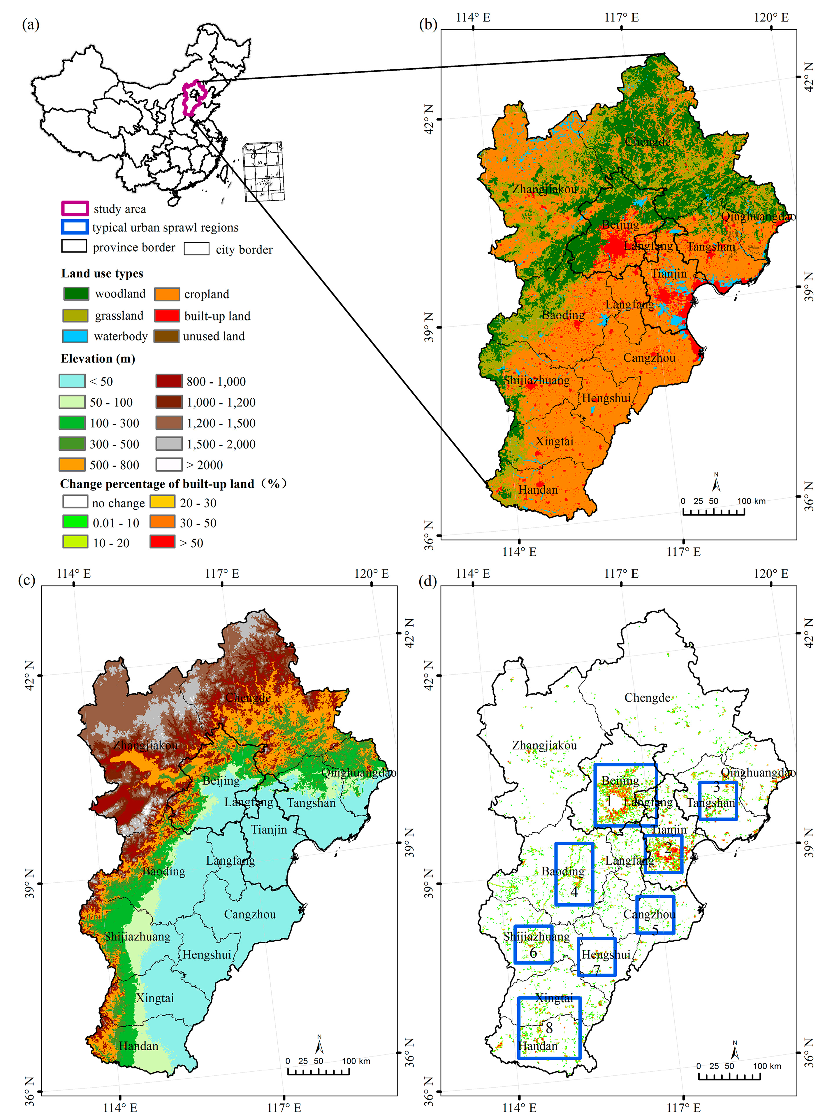
2.1. Study Area

As one of the urban agglomerations experiencing rapid urbanization, the Beijing-Tianjin-Hebei (BTH) region of China was chosen to study thermal effects of urbanization (Figure 1a). The BTH urban agglomeration includes Beijing City, Tianjin City, and 11 cities in Hebei province (Figure 1b), and it is currently defined as the political, cultural, and economic center of China. The BTH region is one of the most developed regions in China, it generates over 10% of the total national GDP in 2010 despite covering only about 2.28% of the Chinese territory (about 22 × 104 km2) [50]. In 2010, the population in this area was about 104.6 million, accounting for 7.84% of the Chinese total population. Beijing and Tianjin are two megacities with population more than 10 million, and Hebei is one of important industrial province in northern China. Most of this region is flat to slightly sloping lowland except the mountainous area of Chengde and the northern Zhangjiakou in the northwestern part, and it belongs to the temperate continental monsoon climate with hot-wet summer and cold-dry winter [51]. In the BTH region, cropland is the land use type occupying the largest proportion (about 50%), and woodland accounts for about 21%, while waterbodies is less than 3%. In most cities, cropland is also the dominate land use type around city/town centers (Figure 1a). In recent decades, the BTH urban agglomeration has undergone enormous population increase and economic growth, urban sprawl is prevalent and replacing a mass of surrounding croplands, while seldom woodland and waterbodies [7,52]. Moreover, the winter wheat-summer maize double cropping system is dominant in this region. The typical growing season for winter wheat is from early October to mid-June of the following year, and summer maize is inter-planted in wheat fields at the beginning of June and harvested at the end of September [53,54].

2.2. Data

2.2.1. Land Use and DEM Data

We used the National Land Cover/Use Dataset of China (NLCD-China) that our research team developed in this study. This dataset was primarily produced by interpreting Landsat TM/ETM+ satellite remote sensing data. The classification scheme includes six first-class land use types: cropland, woodland, grassland, water bodies, built-up land, and unused land. Moreover, there were 25 second-class land use types such as paddy fields, dry land, lakes, streams, and rivers, more information can be found in [55,56]. In this study, we used the land use grid proportion data with 1 km × 1 km resolution in 2000 and 2010. Field survey based validation indicated that the classification accuracy for each land use type was over 90% [55,57]. Digital Elevation Model (DEM) data was derived from the Space Shuttle Radar and Topography Mission (SRTM).

2.2.2. MODIS data

We used the 8-day Emissivity/LST products (Version 005) from MODIS with 1 km resolution from the Land Processes Distributed Active Archive Center (http://modis-land.gsfc.nasa.gov/). The LST was retrieved from clear-sky (99% confidence) observations using a generalized split-window algorithm [58]. MODIS provides observation data regarding the Earth four times a day, the overpass time of Terra is around 10:30 (local solar time) in its descending mode and 22:30 in its ascending mode, while the overpass time of Aqua is around 13:30 in its ascending mode and 01:30 in its descending mode. The LST products derived from the Terra (MOD11A2) and Aqua (MYD11A2) instruments from 2002/185 (year/DOY) to 2011/361 were included in this study to generate month, seasonal, and annual LST datasets. To ensure four observations per day, the MODIS datasets before 2002/185 were not included for fewer than four observations per day. MODIS LST datasets have been widely validated to have an accuracy of less than 1 K in most cases [59].
Snow cover data (MOD10A2) (http://nsidc.org/data/MOD10A2) were provided by National Snow and Ice Data Center (NSIDC). The 8-day 500 m snow cover product has a high accuracy of more than 93% [60]. The time range was the same with the albedo described in the following section for retrieving snow-free albedo.

2.2.3. GLASS Data

Compared with MODIS albedo and LAI datasets, the Global LAnd Surface Satellite (GLASS) albedo and LAI datasets are gapless and continuous, and have similar accuracy to MODIS products. Therefore, we used the albedo and LAI datasets of GLASS products (http://glcf.umd.edu/data/) for analysis of urbanization effects. The GLASS broadband albedo (including visible and NIR spectrum) products show a reasonable consistency with the magnitude and trend of the ground measurements by direct comparison with ground measurements at a set of homogeneous FLUXNET sites, with a bias of less than 0.001 and an RMSE of less than 0.05 for clear days [61]. Previous study also showed high consistency of GLASS and MODIS (or CYCLOPES) LAI values by direct comparison with 20 ground-measured LAI reference maps at 17 sites, with an R-square of 0.76 and RMSE of 0.51 [62,63,64]. The 8-day GLASS albedo products (GLASS02A06 V3, 2000/065–2010/361) and LAI products (GLASS01A01 V3, 2001/001–2011/361) with 1 km resolution were used in this study.

2.3. Methods

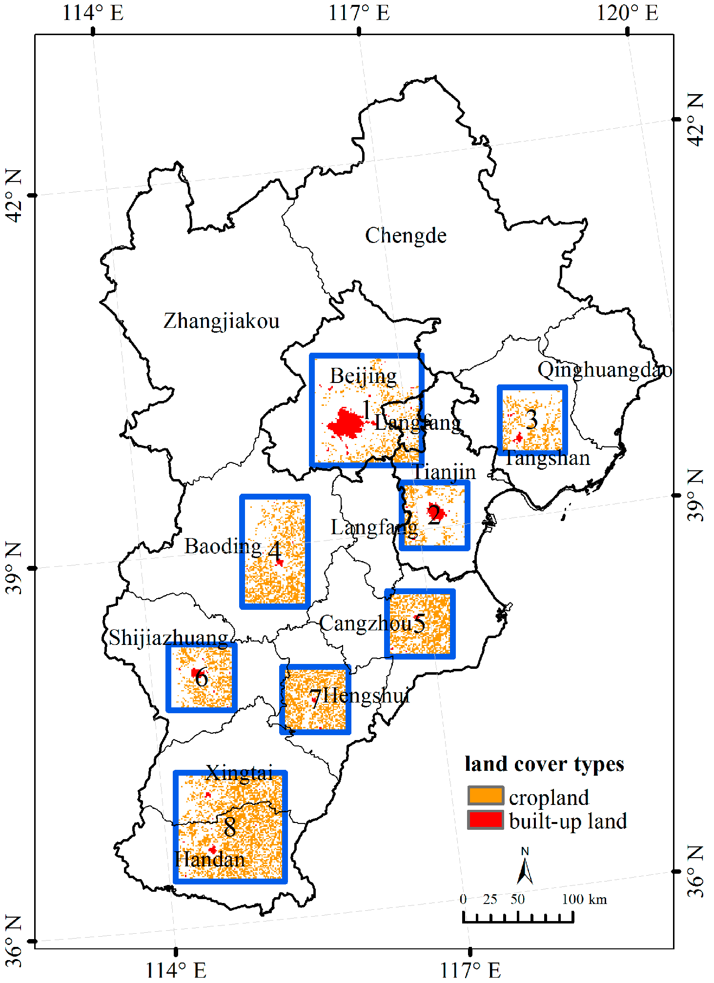
2.3.1. Typical Urban Sprawl Regions

Cropland is the main land cover type around cities and towns in the BTH region, and it is also the most converted type in the urbanization process; thus, it is proper to measure the thermal effects of urbanization by comparing LST of built-up land and nearby croplands. In order to quantitatively measure the thermal effects of urbanization, a set of specific urban and rural paired regions were chosen to compare the LST difference between urban and nearby cropland areas, following the below four principles: (1) Selected regions had undergone significant urban expansions; (2) The spatial distribution of the selected regions were throughout the study area to represent the entire region; (3) In the selected regions, conversion of cropland to built-up land has occurred; (4) There were sufficient optimal values of biophysical parameters in the chosen regions to ensure the reliability of statistical results. Based on these principles, a total of eight typical areas were chosen finally (Figure 1d). Regions No. 1 and No. 8 had a size of 100 km × 100 km, following with No. 4 region of 100 km × 60 km and the rest regions of 60 km × 60 km. The eight chosen typical regions include 10 of 13 cities in the study area, representing the majority of the urban expansion area. The remaining three northern cities were not chosen for less urban expansion and rare optimal values of the biophysical parameters.

2.3.2. Optimal Biophysical Parameters Extraction

Optimal surface parameter values were extracted following three steps: (1) Pure and unchanged grids of built-up land and cropland were selected when the area proportion of this land cover type was greater than or equal to 90%, and their proportion did not change during 2000–2010, and elevation differences between cropland and built-up land ranged within ±120 m in the same typical urban sprawl region (Figure 2); (2) Typical and accurate biophysical values of specific land cover type were obtained by processing original data through quality control flag information. Original 500 m NSIDC snow-cover data (MOD10A2) was first resampled to 1 km using the nearest neighboring method for matching the albedo data. Optimal snow-free broadband white-sky albedos of eight days were obtained by choosing albedo data with a QC flag of 0 (best quality) in GLASS02A06 datasets and snow-free condition according to the NSIDC snow-cover data. Optimal LAI values were obtained by choosing LAI data with a QC flag of 0 (best quality) in GLASS01A01 datasets. High-quality LST values of cropland were obtained by choosing values with LST Error Flag of 0 in MOD11A2/MYD11A2 datasets, yet LST values of built-up land extraction were different, they were obtained by choosing values with LST Error Flag of 0 and 1 for following calculation and analysis. Finally, four times of LST data over built-up land and cropland in a whole day were extracted. (3) The 8-day extracted grid values (LST, Albedo, and LAI) in about 10 years were averaged to eliminate inter-annual variation, and then 8-day zonal average values in typical urban sprawl regions were calculated. Finally, monthly and seasonal values for specific land cover type were acquired based on 8-day zonal average values. The four seasons were defined as spring (March to May), summer (June to August), autumn (September to November), and winter (December to February).

2.3.3. Analysis

In this study, SUHII was defined as the LST differences between pure and unchanged built-up land and cropland at specific observation time in a specific region.
S U H I I ( t ) = L S T ( u r b a n , t ) L S T ( c r o p l a n d , t )
where LST(urban,t) is LST of pure unchanged built-up land at observation time t, and LST(cropland,t) is LST of pure unchanged cropland at observation time t, SUHI(t) is the SUHII at observation time t.
Four times corresponding to MODIS observation times were adopted for SUHII analysis, daytime LST values of built-up land/cropland were obtained by averaging ones at 10:30 and 13:30, while nighttime LST values of built-up land/cropland were obtained by averaging ones at 22:30 and 1:30 local time, then daytime/night SUHII could be obtained according to Equation (1). As two key biophysical variables of radiation budget and energy balance, monthly mean LAI difference (∆LAI) and albedo difference (∆albedo) between built-up land and cropland were applied to uncover the drivers of monthly mean daytime and nighttime SUHII. Moreover, cropland daytime/nighttime LST during the calculation of SUHII was defined as background daytime/nighttime LST. Dependence of daytime/nighttime SUHII on background daytime/nighttime LST was also implemented [43].

3. Results

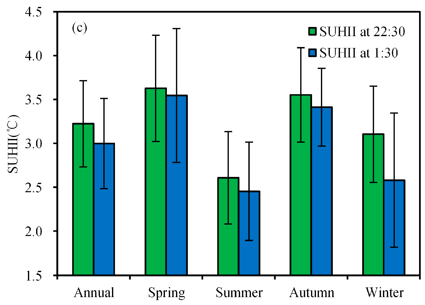
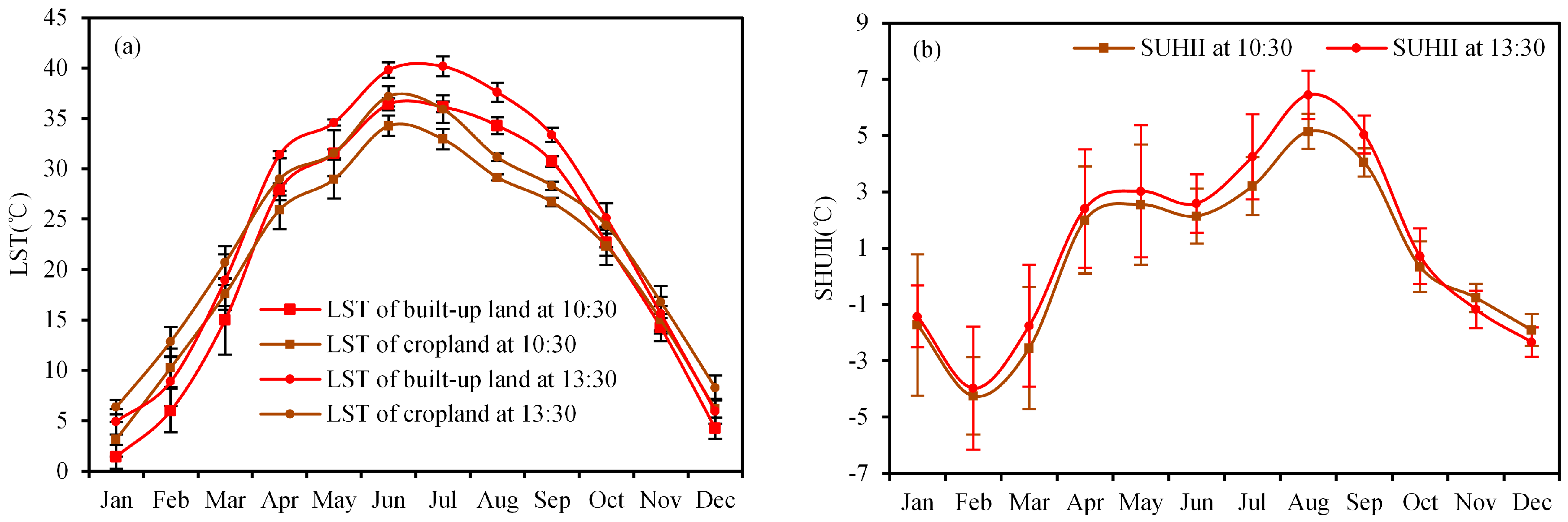
3.1. Seasonal Variations of SUHII
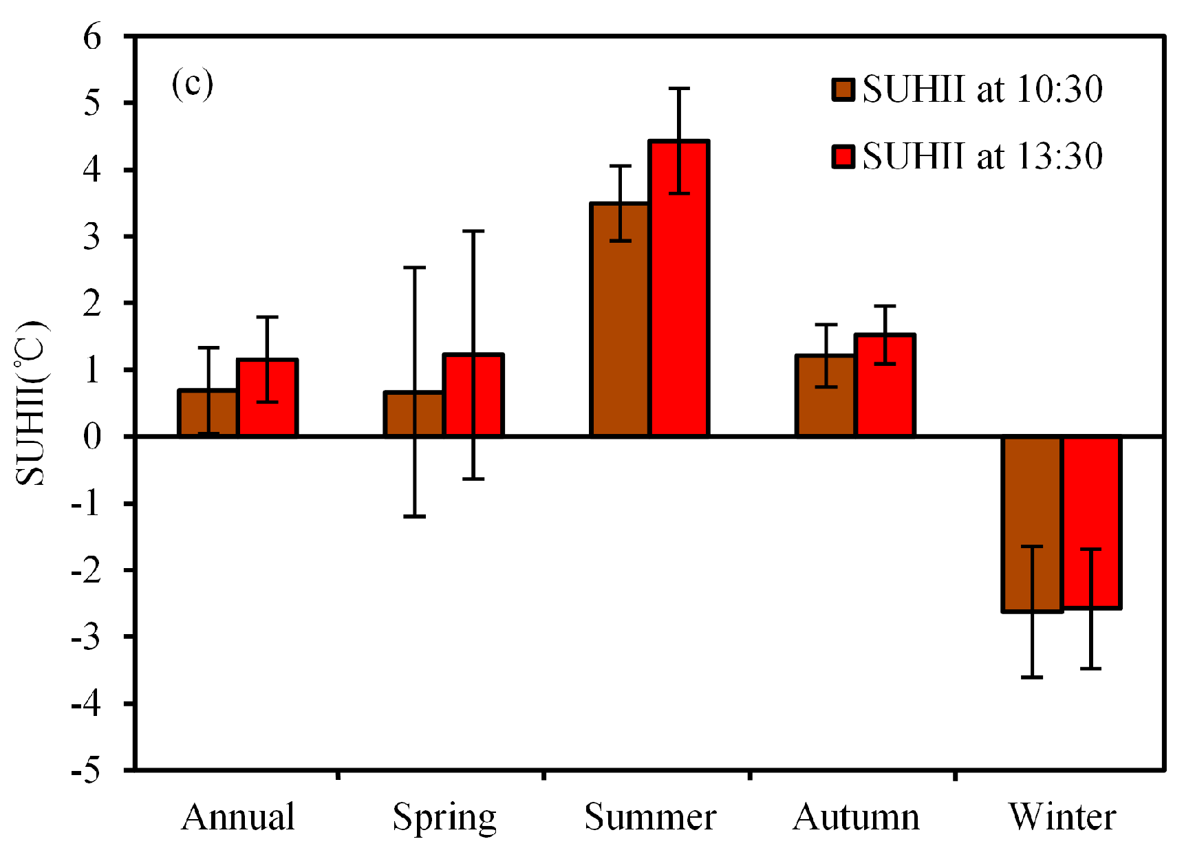
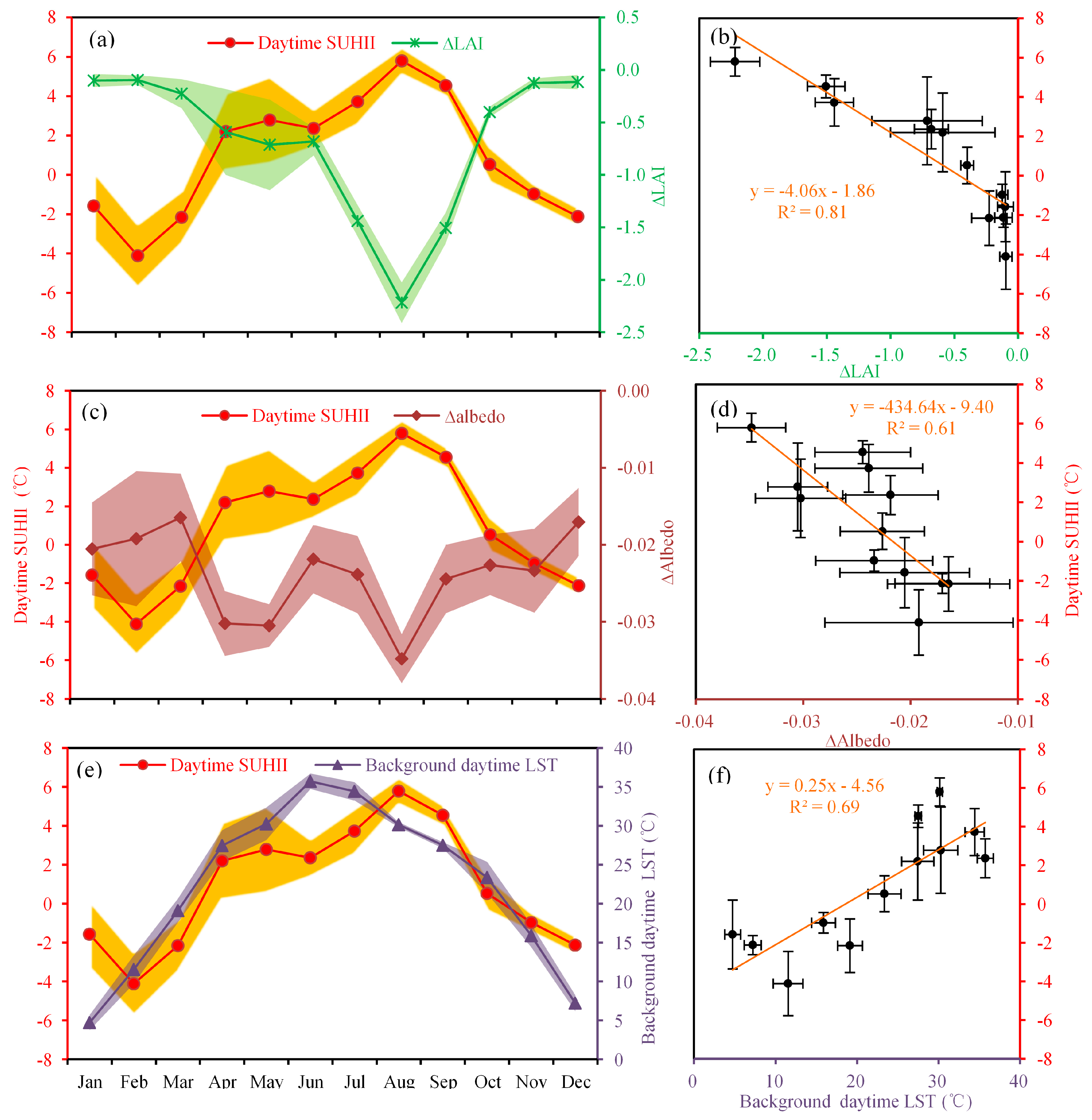
3.1.1 Daytime SUHII

The variations in monthly daytime LST in both built-up land and cropland showed unimodal patterns across the year (Figure 3a). From January to June/July, LST increased, then decreased, and the LST values at 13:30 were significantly higher than that at 10:30 in a whole year. Large monthly and seasonal variations of SUHII were observed during daytime in the BTH region (Figure 3b,c). From April to October, daytime SUHII was positive, showing two peaks in May and August, and with the highest surface urban heat island phenomenon in August. However, in the other five months, the daytime SUHII was negative, showing urban cool island phenomenon in these months. The SUHII at 13:30 was almost higher than that at 10:30 in the whole year, with the exception of November and December. From the perspective of seasons, summer was the season experiencing largest SUHII in the daytime, reaching about 4 °C. In summer, SUHII was 3.50 ± 0.57 °C at 10:30 and 4.43 ± 0.79 °C at 13:30. Spring and autumn also suffered from SUHI phenomenon, whose intensity was much lower than summer, less than 2 °C. However, the daytime SUHII in winter was different from other three seasons, showing negative values both at 10:30 and 13:30. As a whole, annual daytime SUHII was 0.91 ± 0.59 °C, and SUHII increased from 0.68 ± 0.64 °C at 10:30 to 1.15 ± 0.64 °C at 13:30.

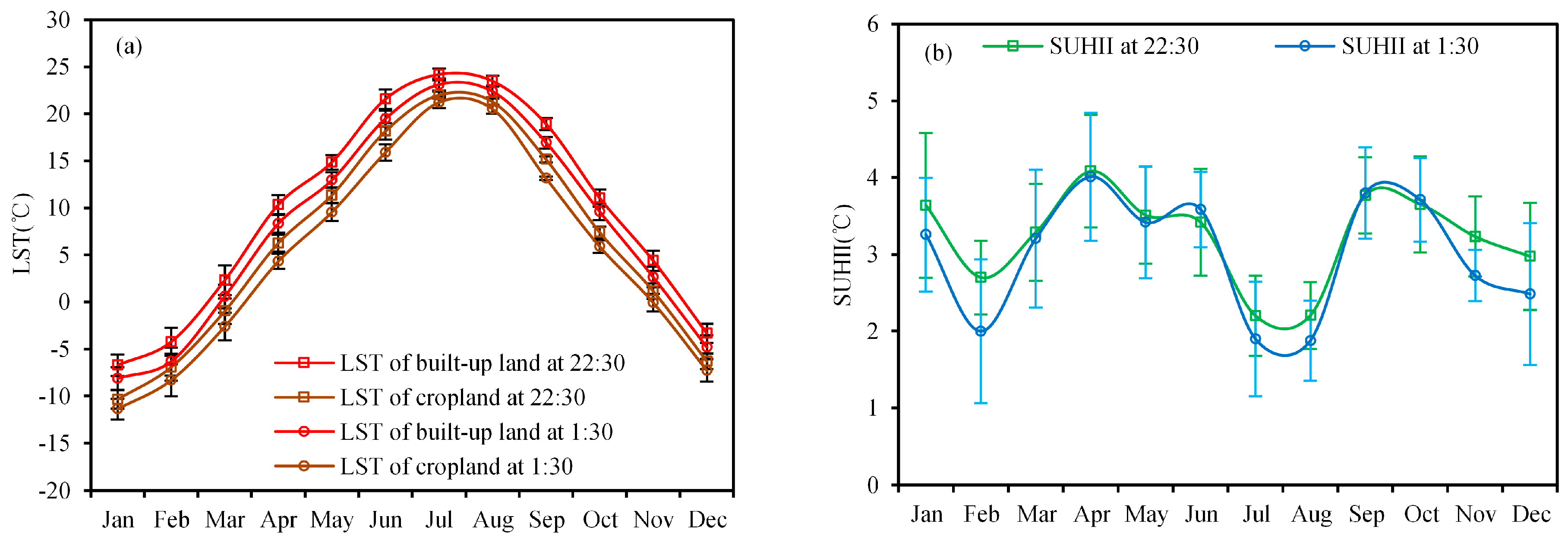
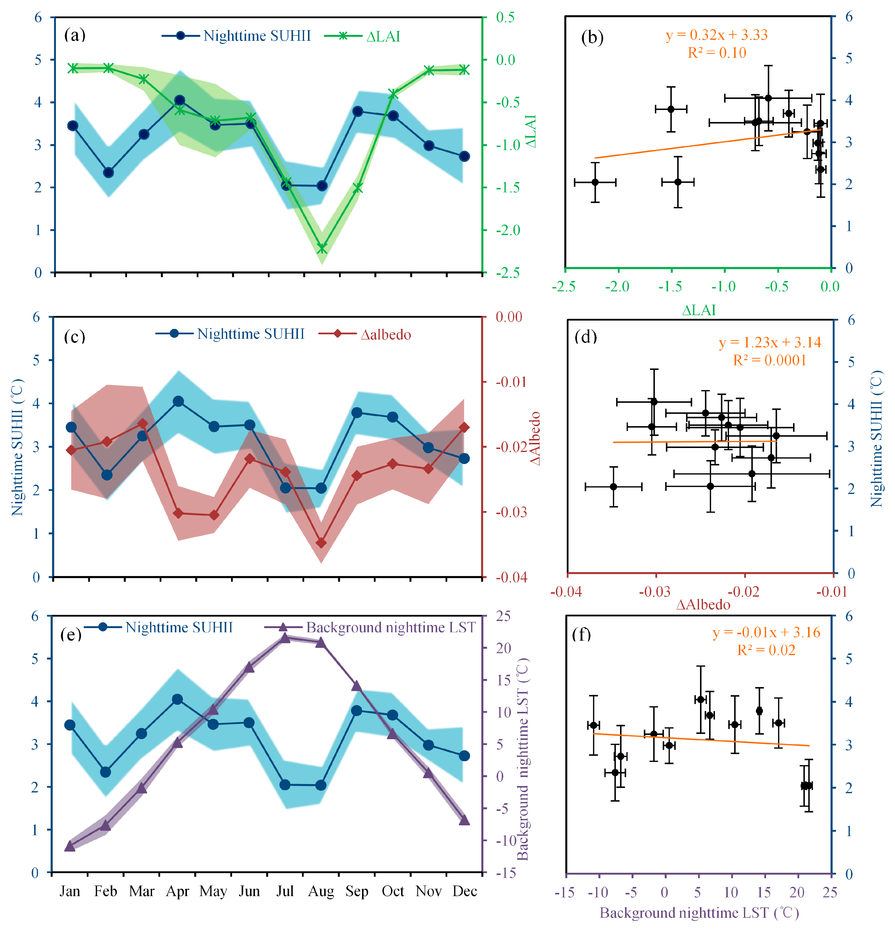
3.1.2. Nighttime SUHII

The variations in monthly nighttime LST in both built-up land and cropland also showed unimodal patterns across the year, similar to that in daytime (Figure 4a). From January to July, LST increased, then decreased, and LST values at 22:30 were significantly higher than that at 1:30 in a whole year for both built-up land and cropland. Compared with daytime SUHII, monthly and seasonal variations of SUHII were found to be more stable during nighttime in the BTH region (Figure 4b,c). In the 12 months, nighttime SUHII was always positive, showing stable apparent SUHI phenomenon at nighttime. And the SUHII at 22:30 was higher than that at 1:30 in all seasons as well as most of the months. On the contrary to daytime SUHII, summer was the season experiencing smallest nighttime SUHII (only 2.53 ± 0.54 °C), with 2.61 ± 0.53 °C at 22:30 and 2.45 ± 0.56 °C at 1:30, which was much lower than daytime SUHII in summer. In spring, autumn and winter, the nighttime SUHI phenomenon was always remarkable (SUHII > 3 °C), larger than corresponding daytime SUHII. As a whole, annual nighttime SUHII was 3.11 ± 0.48 °C, and more remarkable at 22:30 (3.22 ± 0.49 °C) than that at 1:30 (3.00 ± 0.51 °C).

3.2. Driving Forces of SUHII Seasonal Variations

As illustrated in Figure 5, the monthly mean daytime SUHII were closely related to monthly mean ∆LAI, ∆albedo, and background daytime LST. When cropland is converted to built-up land, LAI will decrease in the whole year, especially in May and August. Monthly mean daytime SUHII is negatively and significantly correlated with monthly mean ∆LAI (r = −0.90, p < 0.001), and the two daytime SUHII peaks in May and August correspond to the two troughs of ∆LAI. The highest SUHII in August was corresponding to the largest LAI difference. Moreover, albedo decreases in the whole year along with built-up land occupying cropland, especially in May and August. Relationships between monthly mean daytime SUHII and monthly mean ∆albedo were similar with that of ∆LAI (r = −0.78, p < 0.01). Two daytime SUHII peaks in May and August were also just corresponding to the two troughs of ∆albedo. Meanwhile, monthly background daytime LST was positively correlated with monthly SUHII (r = 0.83, p < 0.01). The month experiencing highest SUHII did not correspond to the highest month experiencing highest background daytime LST (Figure 5), indicating that monthly change of daytime SUHII was not related to a single factor, ∆LAI and ∆albedo would exert influences on the SUHII simultaneously. According to multiple linear regression, combined effects of monthly mean ∆LAI, ∆albedo, and background daytime LST could explain a significantly larger part of the SUHII variation (R2 = 0.92, p < 0.001). As a whole, the seasonal variation of daytime SUHII was affected by synthetic effects of ∆LAI, ∆albedo, background daytime LST and other factors, and variation of ∆LAI is main driver of variation of daytime SUHII with higher explanation rate (R2 = 0.81) compared with variation of ∆albedo (R2 = 0.61) and background daytime LST (R2 = 0.69).
In contrast, relationships between monthly mean nighttime SUHII and monthly mean ∆LAI/∆albedo/background nighttime LST were insignificant (Figure 6). That means the driving forces of seasonal variations of nighttime SUHII were other factors than variations of ∆LAI, ∆albedo, or background nighttime LST, which was different from that of daytime SUHII. However, in growing seasons from April to September, we can also see high consistency as for monthly mean nighttime SUHII and monthly mean ∆LAI/∆albedo, especially in May and August, all showing unified troughs.

4. Discussion

4.1 Possible Mechanisms of Seasonal SUHII Variations

As a whole, the SUHII seasonal variation pattern was consistent with previous studies. The daytime SUHII in summer was the strongest, while daytime SUHII in winter showed a contrary urban cool island phenomenon. This strongest daytime SUHI phenomenon in summer from this study is consistent with previous studies about most of the China cities [40,41], Seoul and Tokyo [38], most of the central European cities [43], and most of the USA cities [28,65]. However, the cities with surface urban cool island are usually distributed in Northern China [40,41] and high latitudes of the Northern Hemisphere (e.g., 55°N–60°N) [10]. The variation in monthly mean daytime SUHII mainly resulted from monthly mean ∆albedo and vegetation change (∆LAI), which varied a lot across the whole year (Figure 5). On the one hand, due to multiple internal reflections resulting from “canopy” geometry of numerous multi-story buildings, urban areas had lower albedo than rural croplands (Figure 5); thus, urban area absorbed more solar radiation, especially in summer with the highest solar radiation in a year. On the other hand, vegetation played a vital role in partitioning sensible heat and latent heat, which was a critical factor influencing UHI. Original land surface with a large amount of vegetation was exploited for residential or transportation lands with less vegetation, causing more sensible heat and less latent heat, thus summer experienced strongest SUHII.
In the BTH region, two daytime SUHII peaks in May and August were found (Figure 5), and this was relevant with the winter wheat-summer maize double cropping system in this region. That showed the control of agriculture practices on vegetation activity and daytime SUHII, consistent with previous study [40]. In August (May), summer maize (winter wheat) was in peak growing stage, owing high LAI and evapotranspiration to cool the surface; while it was the contrary in the urban areas with high sensible heat energy to heat the surface, thus exaggerating the SUHI effect. Moreover, the higher daytime SUHII in August than May was most probably attributed to higher LAI of summer maize than that of winter wheat.
Few studies attempted to explain winter daytime urban cool island, Wang et al. [66] tried to explain it by simulating LST assigning specific thermal inertia values to soil (882 W·s1/2·m−2·K−1) and urban (concrete) (1428 W·s1/2·m−2·K−1) types, and they found lower thermal inertia of dry bare soil in the rural areas can explain the negative SUHII in winter. In winter, land surface is mainly covered by bare soil with sparse vegetation, thus it is conducive to increase LST than urban areas, and in turn lead to the urban cool island. More studies should be done to discover the underlying mechanisms of this urban cool island phenomenon.
With regard to nighttime SUHII, it was greater than daytime SUHII except for summer, and the monthly and seasonal variations of nighttime SUHII were more stable than that of daytime (Figure 4), which was also found in the cities of northern China [40,66], but different from most of the US cities [28] and global mean trend deduced from 419 global big cities [46]. In the BTH region, monthly mean nighttime SUHII was not significantly correlated with monthly mean ∆LAI/∆albedo/background nighttime LST, suggesting different driving mechanism compared with daytime SUHII. It is possibly because nighttime SUHI mainly resulted from the higher thermal admittance of building materials in urban areas than rural areas, which does not change significantly across seasons [29]. Another key factor affecting nighttime SUHII is anthropogenic heat emissions [67,68] from appliances, transportation systems and infrastructures, factories and other human activities, which exist all year around.
Another interesting phenomenon was that daytime SUHII was generally increasing along with the background LST increase, showing significant dependence of daytime SUHII on background LST. This phenomenon meant that when background LST increased, urban area LST experienced faster increase than the nearby rural areas, similar with the heat wave exaggeration results on SUHII [69,70]. In our study, the SUHII reached a peak at 13:30 in summer for the two MODIS daytime observation times. With the increase of background LST from 10:30 to 13:30, urban areas received more incoming shortwave radiation and longwave radiation compared to near rural areas, resulting in more absorbed radiation. Moreover, sensible heat increased more significantly at urban areas due to more impervious materials and scarcity of water, while latent heat increased more significantly at the rural areas due to abundant vegetation and water [70].

4.2. Uncertainties

Although MODIS LST has been validated with a high accuracy, it is mostly over homogeneous surfaces; validation over heterogeneous surfaces such as urban areas remains uncertain [71]. Emissivity estimation of urban areas is easily biased for mixing components, intra-class variation [72,73]. Therefore, LST errors in urban areas may be slightly larger due to large uncertainties in surface emissivity, and this uncertainty will pass on the SUHII calculation. In addition, LST quality control would also have impacts on SUHII as mentioned in study of [74]. Another uncertainty is the chosen method of urban and rural areas for SUHII calculation. As shown in the study of [42], results of different calculation methods (about eleven methods in total) of SUHII show weak correlations. In our study, the SUHII indicator is chosen as LST differences between pure and unchanged urban and cropland pixels to avoid non-concurrency between land cover data and LST data, which is different from previous studies. We also chose LST data of high accuracy through filtering using quality control flag to enable the SUHII calculation more accurate.
Although the pattern of daytime SUHII was consistent with prior research and with less uncertainty [28,38,40,41,43,65], relatively large uncertainty existed in the pattern of nighttime SUHII. The nighttime SUHII in summer was lowest, which was consistent with most of the previous studies [40,66,75], but not consistent with the study of [76]. Nighttime SUHII in spring was the strongest in this study, which was different from summer in the study of [76] and winter in the studies of [40,66,75]. The differences may be due to different SUHII calculation methods [42] as well as LST quality control [74]. Furthermore, relatively limited optimal winter LST values may increase the winter SUHII uncertainty, and our study was for the multi-year average situation, not for a single year [76], thus inter-annual variations may affect the SUHII pattern. Additionally, the variations in city size and latitudes where cities are located could also affect the mechanism of the seasonal variation of SUHII [28,43,65]. Additional studies need to explore this in the future.

5. Conclusions

In this study, based on satellite remote sensing LST data and selected pure and unchanged urban and nearby cropland pixels, we assessed the seasonal variations of daytime and nighttime SUHII and established its relations with the seasonal variations of ∆LAI, ∆albedo, and background LST in the BTH region. In general, there were significant different patterns of daytime and nighttime SUHII. Summer daytime SUHII (about 4 °C) was more evident than other seasons while winter underwent urban cool island. May and August were two months that experienced daytime SUHII peaks, and August was the month suffering from strongest UHI phenomenon greater than 5 °C. Overall, nighttime SUHII was higher and more stable than daytime except in summer, and SUHII was higher than 2 °C in the whole year. Seasonal variations of daytime SUHII mainly resulted from variations of ∆LAI (R2 = 0.81, p < 0.001) and ∆albedo (R2 = 0.61, p < 0.01). More green space or white roofs are needed to alleviate daytime SUHII. Moreover, background LST increase would also exaggerate the SUHI effect in the daytime. However, correlations between seasonal variations of nighttime SUHII and ∆LAI/∆albedo/background nighttime LST were not significant. More studies are needed from the perspective of surface energy balance in the future.

Acknowledgments

This study is funded by the Key Research Program of Frontier Sciences, the Chinese Academy of Sciences (QYZDB-SSW-DQC005), the “Thousand Youth Talents Plan”, the National Natural Science Foundation of China (41371409, 41401504, 41501484, and 41671425), and the National Key Technology Research and Development Program (2013BAC03B04). We are also grateful to the editors and the anonymous referees for their helpful comments and suggestions.

Author Contributions

J.D., J.L., and G.Z. designed the experiments; G.Z., J.Z., Y.C., and T.H. performed the experiments; G.Z., J.D., Y.C., and X.X. analyzed the data; G.Z., J.D., J.L., and Y.C. wrote the paper. All authors reviewed and polished the manuscript.

Conflicts of Interest

The authors declare no conflict of interest.

References

  1. Liu, Z.; He, C.; Zhou, Y.; Wu, J. How much of the world’s land has been urbanized, really? A hierarchical framework for avoiding confusion. Landsc. Ecol. 2014, 29, 763–771. [Google Scholar] [CrossRef]
  2. United Nations. World Urbanization Prospects: The 2014 Revision; United Nations Department of Economics and Social Affairs, Population Division: New York, NY, USA, 2015. [Google Scholar]
  3. Schneider, A.; Friedl, M.A.; Potere, D. A new map of global urban extent from MODIS satellite data. Environ. Res. Lett. 2009, 4, 044003. [Google Scholar] [CrossRef]
  4. Seto, K.C.; Güneralp, B.; Hutyra, L.R. Global forecasts of urban expansion to 2030 and direct impacts on biodiversity and carbon pools. PNAS 2012, 109, 16083–16088. [Google Scholar] [CrossRef] [PubMed]
  5. Deng, X.; Huang, J.; Rozelle, S.; Zhang, J.; Li, Z. Impact of urbanization on cultivated land changes in China. Land Use Policy 2015, 45, 1–7. [Google Scholar] [CrossRef]
  6. He, C.; Liu, Z.; Tian, J.; Ma, Q. Urban expansion dynamics and natural habitat loss in China: A multiscale landscape perspective. Glob. Chang. Biol. 2014, 20, 2886–2902. [Google Scholar] [CrossRef] [PubMed]
  7. Tan, M.; Li, X.; Xie, H.; Lu, C. Urban land expansion and arable land loss in china—A case study of Beijing–Tianjin–Hebei Region. Land Use Policy 2005, 22, 187–196. [Google Scholar] [CrossRef]
  8. Wang, L.; Li, C.; Ying, Q.; Cheng, X.; Wang, X.; Li, X.; Hu, L.; Liang, L.; Yu, L.; Huang, H.; et al. China’s urban expansion from 1990 to 2010 determined with satellite remote sensing. Chin. Sci. Bull. 2012, 57, 2802–2812. [Google Scholar] [CrossRef]
  9. Chase, T.N.; Pielke, R.A.; Kittel, T.G.F.; Nemani, R.; Running, S.W. Sensitivity of a general circulation model to global changes in leaf area index. J. Geophys. Res.: Atmos. 1996, 101, 7393–7408. [Google Scholar] [CrossRef]
  10. Jin, M.; Dickinson, R.E.; Zhang, D. The footprint of urban areas on global climate as characterized by MODIS. J. Clim. 2005, 18, 1551–1565. [Google Scholar] [CrossRef]
  11. Sun, J.; Wang, X.; Chen, A.; Ma, Y.; Cui, M.; Piao, S. Ndvi indicated characteristics of vegetation cover change in China's metropolises over the last three decades. Environ. Monit. Assess. 2011, 179, 1–14. [Google Scholar] [CrossRef] [PubMed]
  12. Zhao, L.; Lee, X.; Smith, R.B.; Oleson, K. Strong contributions of local background climate to urban heat islands. Nature 2014, 511, 216–219. [Google Scholar] [CrossRef] [PubMed]
  13. Zhao, S.; Liu, S.; Zhou, D. Prevalent vegetation growth enhancement in urban environment. PNAS 2016, 113, 6313–6318. [Google Scholar] [CrossRef] [PubMed]
  14. Guo, W.; Wang, X.; Sun, J.; Ding, A.; Zou, J. Comparison of land–atmosphere interaction at different surface types in the mid- to lower reaches of the yangtze river valley. Atmos. Chem. Phys. 2016, 16, 9875–9890. [Google Scholar] [CrossRef]
  15. Hu, Y.; Jia, G.; Pohl, C.; Zhang, X.; van Genderen, J. Assessing surface albedo change and its induced radiation budget under rapid urbanization with Landsat and GLASS data. Theor. Appl. Climatol. 2015, 123, 711–722. [Google Scholar] [CrossRef] [Green Version]
  16. Arnfield, A.J. Two decades of urban climate research: A review of turbulence, exchanges of energy and water, and the urban heat island. Int. J. Climatol. 2003, 23, 1–26. [Google Scholar] [CrossRef]
  17. Oke, T.R. City size and the urban heat island. Atmos. Environ. 1973, 7, 769–779. [Google Scholar] [CrossRef]
  18. Zhou, D.; Zhao, S.; Liu, S.; Zhang, L. Spatiotemporal trends of terrestrial vegetation activity along the urban development intensity gradient in China's 32 major cities. Sci. Total Environ. 2014, 488, 136–145. [Google Scholar] [CrossRef] [PubMed]
  19. Milesi, C.; Elvidge, C.D.; Nemani, R.; Running, S.W. Assessing the impact of urban land development on net primary productivity in the southeastern United States. Remote Sens. Environ. 2003, 86, 401–410. [Google Scholar] [CrossRef]
  20. Kalnay, E.; Cai, M. Impact of urbanization and land-use change on climate. Nature 2003, 423, 528–531. [Google Scholar] [CrossRef] [PubMed]
  21. Zhou, L.; Dickinson, R.E.; Tian, Y.; Fang, J.; Li, Q.; Kaufmann, R.K.; Tucker, C.J.; Myneni, R.B. Evidence for a significant urbanization effect on climate in China. PNAS USA 2004, 101, 9540–9544. [Google Scholar] [CrossRef] [PubMed]
  22. Grimm, N.B.; Faeth, S.H.; Golubiewski, N.E.; Redman, C.L.; Wu, J.; Bai, X.; Briggs, J.M. Global change and the ecology of cities. Science 2008, 319, 756–760. [Google Scholar] [CrossRef] [PubMed]
  23. Han, L.; Zhou, W.; Li, W.; Li, L. Impact of urbanization level on urban air quality: A case of fine particles (PM2.5) in Chinese cities. Environ. Pollut. 2014, 194, 163–170. [Google Scholar] [CrossRef] [PubMed]
  24. Shandas, V.; Duh, J.; Chang, H.; George, L.A. Rates of urbanisation and the resiliency of air and water quality. Sci. Total Environ. 2008, 400, 238–256. [Google Scholar]
  25. De Poel, E.V.; Odonnell, O.; Van Doorslaer, E. Is there a health penalty of china's rapid urbanization? Health Econ. 2012, 21, 367–385. [Google Scholar] [CrossRef] [PubMed]
  26. Gong, P.; Liang, S.; Carlton, E.J.; Jiang, Q.; Wu, J.; Wang, L.; Remais, J.V. Urbanisation and health in China. The Lancet 2012, 379, 843–852. [Google Scholar] [CrossRef]
  27. Sophie, E.; Stefan, K. Urbanization and health in developing countries: A systematic review. World Health Popul. 2014, 15, 7–20. [Google Scholar]
  28. Imhoff, M.L.; Zhang, P.; Wolfe, R.E.; Bounoua, L. Remote sensing of the urban heat island effect across biomes in the continental USA. Remote Sens. Environ. 2010, 114, 504–513. [Google Scholar] [CrossRef]
  29. Oke, T.R. The energetic basis of the urban heat island. Q. J. R. Meteorolog. Soc. 1982, 108, 1–24. [Google Scholar] [CrossRef]
  30. Azevedo, J.A.; Chapman, L.; Muller, C.L. Quantifying the daytime and night-time urban heat island in birmingham, uk: A comparison of satellite derived land surface temperature and high resolution air temperature observations. Remote Sens. 2016, 8, 153. [Google Scholar] [CrossRef]
  31. Martin, P.; Baudouin, Y.; Gachon, P. An alternative method to characterize the surface urban heat island. Int. J. Biometeorol. 2015, 59, 849–861. [Google Scholar] [CrossRef] [PubMed]
  32. Oke, T.R. The heat island of the urban boundary layer: Characteristics, causes and effects. In Wind Climate in Cities; Cermak, J.E., Davenport, A.G., Plate, E.J., Viegas, D.X., Eds.; Springer: Dordrecht, The Netherlands, 1995; pp. 81–107. [Google Scholar]
  33. Voogt, J.A.; Oke, T.R. Thermal remote sensing of urban climates. Remote Sens. Environ. 2003, 86, 370–384. [Google Scholar] [CrossRef]
  34. Fu, P.; Weng, Q. Consistent land surface temperature data generation from irregularly spaced Landsat imagery. Remote Sens. Environ. 2016, 184, 175–187. [Google Scholar] [CrossRef]
  35. Haashemi, S.; Weng, Q.; Darvishi, A.; Alavipanah, S.K. Seasonal variations of the surface urban heat island in a semi-arid city. Remote Sens. 2016, 8, 352. [Google Scholar] [CrossRef]
  36. Shen, H.; Huang, L.; Zhang, L.; Wu, P.; Zeng, C. Long-term and fine-scale satellite monitoring of the urban heat island effect by the fusion of multi-temporal and multi-sensor remote sensed data: A 26-year case study of the City of Wuhan in China. Remote Sens. Environ. 2016, 172, 109–125. [Google Scholar] [CrossRef]
  37. Tomaszewska, M.; Henebry, G. Urban–rural contrasts in central-eastern european cities using a MODIS 4 micron time series. Remote Sens. 2016, 8, 924. [Google Scholar] [CrossRef]
  38. Tran, H.; Uchihama, D.; Ochi, S.; Yasuoka, Y. Assessment with satellite data of the urban heat island effects in Asian mega cities. Int. J. Appl. Earth Obs. Geoinf. 2006, 8, 34–48. [Google Scholar] [CrossRef]
  39. Anniballe, R.; Bonafoni, S.; Pichierri, M. Spatial and temporal trends of the surface and air heat island over milan using MODIS data. Remote Sens. Environ. 2014, 150, 163–171. [Google Scholar] [CrossRef]
  40. Zhou, D.; Zhang, L.; Li, D.; Huang, D.; Zhu, C. Climate–vegetation control on the diurnal and seasonal variations of surface urban heat islands in China. Environ. Res. Lett. 2016, 11, 074009. [Google Scholar] [CrossRef]
  41. Zhou, D.; Zhao, S.; Liu, S.; Zhang, L.; Zhu, C. Surface urban heat island in China's 32 major cities: Spatial patterns and drivers. Remote Sens. Environ. 2014, 152, 51–61. [Google Scholar] [CrossRef]
  42. Schwarz, N.; Lautenbach, S.; Seppelt, R. Exploring indicators for quantifying surface urban heat islands of european cities with MODIS land surface temperatures. Remote Sens. Environ. 2011, 115, 3175–3186. [Google Scholar] [CrossRef]
  43. Zhou, B.; Rybski, D.; Kropp, J.P. On the statistics of urban heat island intensity. Geophys. Res. Lett. 2013, 40, 5486–5491. [Google Scholar] [CrossRef]
  44. Lazzarini, M.; Molini, A.; Marpu, P.R.; Ouarda, T.B.M.J.; Ghedira, H. Urban climate modifications in hot desert cities: The role of land cover, local climate, and seasonality. Geophys. Res. Lett. 2015, 42, 9980–9989. [Google Scholar] [CrossRef]
  45. Clinton, N.; Gong, P. Modis detected surface urban heat islands and sinks: Global locations and controls. Remote Sens. Environ. 2013, 134, 294–304. [Google Scholar] [CrossRef]
  46. Peng, S.; Piao, S.; Ciais, P.; Friedlingstein, P.; Ottle, C.; Breon, F.M.; Nan, H.; Zhou, L.; Myneni, R.B. Surface urban heat island across 419 global big cities. Environ. Sci. Technol. 2012, 46, 696–703. [Google Scholar] [CrossRef] [PubMed]
  47. Cao, C.; Lee, X.; Liu, S.; Schultz, N.; Xiao, W.; Zhang, M.; Zhao, L. Urban heat islands in China enhanced by haze pollution. Nat. Commun. 2016, 7, 12509. [Google Scholar] [CrossRef] [PubMed]
  48. Krehbiel, C.P.; Jackson, T.; Henebry, G.M. Web-enabled landsat data time series for monitoring urban heat island impacts on land surface phenology. IEEE J. Sel. Top. Appl. Earth Obs. Remote Sens. 2016, 9, 2043–2050. [Google Scholar] [CrossRef]
  49. Zhao, S.; Zhou, D.; Liu, S. Data concurrency is required for estimating urban heat island intensity. Environ. Pollut. 2016, 208, 118–124. [Google Scholar] [CrossRef] [PubMed]
  50. National Bureau of Statistics of China (NBSC). China Statistical Yearbook; China Statistics Press: Beijing, China, 2011.
  51. Feng, Z.; Liu, D.; Zhang, Y. Water requirements and irrigation scheduling of spring maize using GIS and Cropwat Model in Beijing-Tianjin-Hebei region. Chinese Geogr. Sci. 2007, 17, 56–63. [Google Scholar] [CrossRef]
  52. Zhang, Z.; Li, N.; Wang, X.; Liu, F.; Yang, L. A comparative study of urban expansion in Beijing, Tianjin and Tangshan from the 1970s to 2013. Remote Sens. 2016, 8, 496. [Google Scholar] [CrossRef]
  53. Sun, H.; Shen, Y.; Yu, Q.; Flerchinger, G.N.; Zhang, Y.; Liu, C.; Zhang, X. Effect of precipitation change on water balance and wue of the winter wheat–summer maize rotation in the north China plain. Agric. Water Manage. 2010, 97, 1139–1145. [Google Scholar] [CrossRef]
  54. Liu, C.; Zhang, X.; Zhang, Y. Determination of daily evaporation and evapotranspiration of winter wheat and maize by large-scale weighing lysimeter and micro-lysimeter. Agric. For. Meteorol. 2002, 111, 109–120. [Google Scholar] [CrossRef]
  55. Zhang, Z.Y.; Wang, X.; Zhao, X.; Liu, B.; Yi, L.; Zuo, L.; Wen, Q.; Liu, F.; Xu, J.; Hu, S. A 2010 update of national land use/cover database of China at 1:100000 scale using medium spatial resolution satellite images. Remote Sens. Environ. 2014, 149, 142–154. [Google Scholar] [CrossRef]
  56. Liu, J.; Liu, M.; Tian, H.; Zhuang, D.; Zhang, Z.; Zhang, W.; Tang, X.; Deng, X. Spatial and temporal patterns of China's cropland during 1990–2000: An analysis based on landsat tm data. Remote Sens. Environ. 2005, 98, 442–456. [Google Scholar] [CrossRef]
  57. Liu, J.; Kuang, W.; Zhang, Z.; Xu, X.; Qin, Y.; Ning, J.; Zhou, W.; Zhang, S.; Li, R.; Yan, C.; et al. Spatiotemporal characteristics, patterns, and causes of land-use changes in China since the late 1980s. J. Geog. Sci. 2014, 24, 195–210. [Google Scholar] [CrossRef]
  58. Wan, Z.; Li, Z.-L. A physics-based algorithm for retrieving land-surface emissivity and temperature from EOS/MODIS data. IEEE Trans. Geosci. Remote Sens. 1997, 35, 980–996. [Google Scholar]
  59. Wan, Z. New refinements and validation of the modis land-surface temperature/emissivity products. Remote Sens. Environ. 2008, 112, 59–74. [Google Scholar] [CrossRef]
  60. Hall, D.K.; Riggs, G.A. Accuracy assessment of the modis snow products. Hydrol. Process. 2007, 21, 1534–1547. [Google Scholar] [CrossRef]
  61. Liu, Q.; Wang, L.; Qu, Y.; Liu, N.; Liu, S.; Tang, H.; Liang, S. Preliminary evaluation of the long-term glass albedo product. Int. J. Digital Earth 2013, 6, 69–95. [Google Scholar] [CrossRef]
  62. Xiang, Y.; Xiao, Z.; Ling, S.; Wang, J.; Song, J. Validation of global land surface satellite (GLASS) leaf area index product. J. Remote Sens. 2014, 18, 573–596. [Google Scholar]
  63. Xiao, Z.; Liang, S.; Wang, J.; Chen, P.; Yin, X.; Zhang, L.; Song, J. Use of general regression neural networks for generating the glass leaf area index product from time-series MODIS surface reflectance. IEEE Trans. Geosci. Remote Sens. 2014, 52, 209–223. [Google Scholar] [CrossRef]
  64. Xiao, Z.; Liang, S.; Wang, J.; Xiang, Y.; Zhao, X.; Song, J. Long-time-series global land surface satellite leaf area index product derived from modis and avhrr surface reflectance. IEEE Trans. Geosci. Remote Sens. 2016, 54, 5301–5318. [Google Scholar] [CrossRef]
  65. Krehbiel, C.; Henebry, G. A comparison of multiple datasets for monitoring thermal time in urban areas over the U.S. Upper Midwest. Remote Sens. 2016, 8, 297. [Google Scholar] [CrossRef]
  66. Wang, K.; Wang, J.; Wang, P.; Sparrow, M.; Yang, J.; Chen, H. Influences of urbanization on surface characteristics as derived from the moderate-resolution imaging spectroradiometer: A case study for the Beijing metropolitan area. J. Geophys. Res. 2007, 112. [Google Scholar] [CrossRef]
  67. Best, M.J.; Grimmond, C.S.B. Key conclusions of the first international urban land surface model comparison project. Bull. Am. Meteorol. Soc. 2015, 96, 805–819. [Google Scholar] [CrossRef]
  68. Feng, J.; Wang, Y.; Ma, Z.; Liu, Y. Simulating the regional impacts of urbanization and anthropogenic heat release on climate across China. J. Clim. 2012, 25, 7187–7203. [Google Scholar] [CrossRef]
  69. Ward, K.; Lauf, S.; Kleinschmit, B.; Endlicher, W. Heat waves and urban heat islands in Europe: A review of relevant drivers. Sci. Total Environ. 2016, 569–570, 527–539. [Google Scholar] [CrossRef] [PubMed]
  70. Li, D.; Sun, T.; Liu, M.; Yang, L.; Wang, L.; Gao, Z. Contrasting responses of urban and rural surface energy budgets to heat waves explain synergies between urban heat islands and heat waves. Environ. Res. Lett. 2015, 10, 054009. [Google Scholar] [CrossRef]
  71. Quan, J.; Zhan, W.; Chen, Y.; Wang, M.; Wang, J. Time series decomposition of remotely sensed land surface temperature and investigation of trends and seasonal variations in surface urban heat islands. J. Geophys. Res.: Atmos. 2016, 121, 2638–2657. [Google Scholar] [CrossRef]
  72. Mitraka, Z.; Chrysoulakis, N.; Kamarianakis, Y.; Partsinevelos, P.; Tsouchlaraki, A. Improving the estimation of urban surface emissivity based on sub-pixel classification of high resolution satellite imagery. Remote Sens. Environ. 2012, 117, 125–134. [Google Scholar] [CrossRef]
  73. Stathopoulou, M.; Cartalis, C.; Petrakis, M. Integrating corine land cover data and landsat tm for surface emissivity definition: Application to the urban area of Athens, Greece. Int. J. Remote Sens. 2007, 28, 3291–3304. [Google Scholar] [CrossRef]
  74. Gawuc, L.; Struzewska, J. Impact of MODIS quality control on temporally aggregated urban surface temperature and long-term surface urban heat island intensity. Remote Sens. 2016, 8, 374. [Google Scholar] [CrossRef]
  75. Quan, J.; Chen, Y.; Zhan, W.; Wang, J.; Voogt, J.; Wang, M. Multi-temporal trajectory of the urban heat island centroid in Beijing, China based on a gaussian volume model. Remote Sens. Environ. 2014, 149, 33–46. [Google Scholar] [CrossRef]
  76. Zhang, J.; Hou, Y.; Li, G.; Yan, H.; Yao, F. The diurnal and seasonal characteristics of urban heat island variation in Beijing City and surrounding areas and impact factors based on remote sensing satellite data. Sci. China Ser. D: Earth Sci. 2005, 48, 220–229. [Google Scholar]
Figure 1. Overview of the study area: (a) Location of the Beijing-Tianjin-Hebei (BTH) urban agglomeration in China; (b) Spatial pattern of land use types; (c) Elevation; (d) Distribution of built-up land expansion (%) during 2000–2010 and the distribution of selected typical urban sprawl areas (blue rectangles).
Remotesensing 09 00121 g001
Figure 2. Distribution of the pure and unchanged urban and cropland pixels, and the selected typical urban sprawl regions (blue rectangles) for surface urban heat island intensity (SUHII) analysis.
Remotesensing 09 00121 g002
Figure 3. Seasonal variations of daytime land surface temperature (LST) and daytime SUHII: (a) Monthly variation of daytime LST for built-up land and cropland; (b) Monthly variation of daytime SUHII; (c) Seasonal variation of daytime SUHII. Error bars represent one standard deviation across the eight typical urban sprawl regions.
Remotesensing 09 00121 g003aRemotesensing 09 00121 g003b
Figure 4. Seasonal variations of nighttime LST and SUHII: (a) Monthly variation of nighttime LST for built-up land and cropland; (b) Monthly variation of nighttime SUHII; (c) Seasonal variation of nighttime SUHII. Error bars represent one standard deviation across the eight typical urban sprawl regions.
Remotesensing 09 00121 g004aRemotesensing 09 00121 g004b
Figure 5. Driving forces of seasonal variations of daytime SUHII: (a) Seasonal variations of daytime SUHII and ∆LAI (leaf area index); (b) Correlations between monthly daytime SUHII and ∆LAI; (c) Seasonal variations of daytime SUHII and ∆albedo; (d) Correlations between monthly daytime SUHII and ∆albedo; (e) Seasonal variations of daytime SUHII and background daytime LST; (f) Correlations between monthly daytime SUHII and background daytime LST. The shaded areas and error bars represent one standard deviation across the eight typical urban sprawl regions.
Remotesensing 09 00121 g005
Figure 6. Driving forces of seasonal variations of nighttime SUHII: (a) Seasonal variations of nighttime SUHII and ∆LAI; (b) Correlations between monthly nighttime SUHII and ∆LAI; (c) Seasonal variations of nighttime SUHII and ∆albedo; (d) Correlations between monthly nighttime SUHII and ∆albedo; (e) Seasonal variations of nighttime SUHII and background nighttime LST; (f) Correlations between monthly nighttime SUHII and background nighttime LST. The shaded areas and error bars represent one standard deviation across the eight typical urban sprawl regions.
Remotesensing 09 00121 g006

