Validation of PROBA-V GEOV1 and MODIS C5 & C6 fAPAR Products in a Deciduous Beech Forest Site in Italy

Abstract

The availability of new fAPAR satellite products requires simultaneous efforts in validation to provide users with a better comprehension of product performance and evaluation of uncertainties. This study aimed to validate three fAPAR satellite products, GEOV1, MODIS C5, and MODIS C6, against ground references to determine to what extent the GCOS requirements on accuracy (maximum 10% or 5%) can be met in a deciduous beech forest site in a gently and variably sloped mountain site. Three ground reference fAPAR, differing for temporal (continuous or campaign mode) and spatial sampling (single points or Elementary Sampling Units—ESUs), were collected using different devices: (1) Apogee (defined as benchmark in this study); (2) PASTIS; and (3) Digital cameras for collecting hemispherical photographs (DHP). A bottom-up approach for the upscaling process was used in the present study. Radiometric values of decametric images (Landsat-8) were extracted over the ESUs and used to develop empirical transfer functions for upscaling the ground measurements. The resulting high-resolution ground-based maps were aggregated to the spatial resolution of the satellite product to be validated considering the equivalent point spread function of the satellite sensors, and a correlation analysis was performed to accomplish the accuracy assessment. PASTIS sensors showed good performance as fAPAR_PASTIS appropriately followed the seasonal trends depicted by fAPAR_APOGEE (benchmark) (R² = 0.84; RMSE = 0.01). Despite small dissimilarities, mainly attributed to different sampling schemes and errors in DHP classification process, the agreement between fAPAR_PASTIS and fAPAR_DHP was noticeable considering all the differences between both approaches. The temporal courses of the three satellite products were found to be consistent with both Apogee and PASTIS, except at the end of the summer season when ground data were more affected by senescent leaves, with both MODIS C5 and C6 displaying larger short-term variability due to their shorter temporal composite period. MODIS C5 and C6 retrievals were obtained with the backup algorithm in most cases. The three green fAPAR satellite products under study showed good agreement with ground-based maps of canopy fAPAR at 10 h, with RMSE values lower than 0.06, very low systematic differences, and more than 85% of the pixels within GCOS requirements. Among them, GEOV1 fAPAR showed up to 98% of the points lying within the GCOS requirements, and slightly lower values (mean bias = −0.02) as compared with the ground canopy fAPAR, which is expected to be only slightly higher than green fAPAR in the peak season.

1. Introduction

Ecosystems are continuously changing due to both natural and anthropic factors. Monitoring biophysical variables is fundamental to describe vegetation dynamics, disturbances, and responses to changing environmental conditions [1]. The Fraction of Absorbed Photosynthetically Active Radiation (fAPAR) is recognized as an Essential Climate Variable (ECV) by the Global Climate Observing System (GCOS) as it has a primary role in estimation of carbon balance [2]. fAPAR is generally defined as the fraction of Photosynthetically Active Radiation (PAR) absorbed by vegetation, where PAR is the solar radiation reaching the vegetation in the wavelength region 400–700 nm [3]. Consequently, fAPAR is the available light energy for plant productivity and thus is strictly related to photosynthesis. It is influenced by illumination condition and varies with sun position, atmospheric conditions, and the relative contributions of the direct and diffuse illumination [4]. The actual or ‘blue-sky’ fAPAR is the sum of two terms, weighted by the diffuse fraction in the PAR domain: the ‘black-sky’ fAPAR related to the direct component of the incident radiation and the ‘white-sky’ fAPAR related to the diffuse component of the incident radiation [5].

The importance of this variable in the vegetation monitoring is related to (1) the fact that is linked both to ecosystem function and structure [6] and (2) the possibility that it can be monitored from space. The growing availability of fAPAR satellite products at a global level make this variable suitable for monitoring vegetation status [7], phenology [8], drought events [9], and land degradation [10]. The productivity of a vegetated surface is related to fAPAR and remotely sensed fAPAR data are widely used as input in carbon productivity models [11,12,13]. One of the most widely used models in the estimation of carbon productivity is the Light Use Efficiency (LUE) model that describes carbon sequestration as a product of a structural term determining light absorption (fAPAR × PAR) and a physiological efficiency term (ε) defining the conversion of solar radiation into biomass or carbon. In this approach, the accuracy fAPAR data used is relevant, as it has a considerable impact on the fluxes estimated by the model [14], even more in those cases when ε is assumed to be constant.

The methods used to monitor fAPAR could be divided into ground and satellite methods. Weiss et al. [4] report that there are primarily four different ground methods, depending on the approximation: (a) assessing fAPAR directly using quantum sensors that measure all the terms of the radiation balance [15]; (b) assessing transmitted PAR using ceptometers that compute the instantaneous fIPAR (fraction of Intercepted PAR) [16]; (c) assessing directional transmittance measurements using digital hemispherical photography (DHP) [5] or LAI-2000 [17]; and (d) simulating fAPAR through a 3D model that accurately takes into account the canopy structure [18]. On the other hand, the major approaches used to estimate fAPAR from remote sensing over a large spatial scale are basically two: (a) empirical models based on relationships between field measurements and satellite-derived vegetation indices as Normalized Difference Vegetation Index (NDVI) [19,20] or EVI [21,22] and (b) physically-based methods by inversion of radiative transfer models (RTM) [23,24]. In the last decades, several satellite-based fAPAR products have been developed from different sensors on a global scale by spatial agencies and earth observation services. This has made various fAPAR products at different temporal and spatial resolutions of the Earth available to the scientific community [25,26,27,28,29,30,31]. In particular, the Copernicus Global Land Service (http://land.copernicus.eu/global/) delivers global LAI, fAPAR, and fCOVER products from SPOT VEGETATION (1999–2014) and PROBA-V observations (2014-present) with a spatial sampling close to 1 km and temporal frequency of 10 days. These products, namely GEOV1 products, were developed to capitalize on existing products and its validation results [31], and were globally validated and compared with existing satellite data and ground reference maps, showing better performance than other satellite products [32]. Since 2000, NASA has delivered MODIS/TERRA fAPAR Collection 5 (C5) products that are produced at 1 km spatial resolution [23,33]. Accuracy improvements from 0.2 to 0.1 of Collection 5 over previous Collection 4 were observed in several studies [34,35,36]. Lastly, the newest version of fAPAR MODIS product is Collection 6 (C6) which is 500 m spatial resolution and contains the entire time series from February 2000 to the present [37]. Recent studies [37,38] aimed to assess product accuracy, uncertainty, and consistency with the previous version. Yan et al. [38] informed about the absence of valid ground truth for fAPAR measurements over deciduous broadleaf forest and recommended more efforts in field measurements to further refine remote sensing data performance in the future. Camacho et al. [32] also pointed out how validation of satellite products is limited by the ground dataset available and that, presently, a small amount of data exists concerning broadleaf evergreen and deciduous forests. Recently, studies aimed to evaluate consistency between fAPAR datasets in forest biomes proved that important differences exist among them and thus further efforts to improve accuracy in carbon models are needed [34,39,40,41]. Subsequently, the availability of new satellite products requires simultaneous efforts in their validation to provide users with a better comprehension of product performances and uncertainties [42]. To reach this goal, ground reference fAPAR datasets are essential. However few sites are equipped to generate measurements of fAPAR useful for the validation of space-borne products [3]. Nevertheless, validation is not simply equivalent to field measurements. An upscaling strategy to extend the in situ measurements and match satellite data resolution is needed in order to properly address the spatial variability of the site at the size of satellite footprints [43]. In situ fAPAR is usually measured using four sensors that simultaneously measure the downwelling and upwelling PAR both below and above the forest canopy, representing a value of the fraction of absorbed PAR by the canopy. Differently from short canopies (e.g., grasslands), access to a tower is required to measure reflected and incident PAR at the top of a tall canopy [40]. Also, collecting ground datasets is resource intensive and mostly limited in spatial and temporal sampling extensions [39]. In this respect, if the in validation of satellite data with accurate field data is generally necessary, that carried out in forest ecosystems is even more valuable and indispensable.

This paper presents a validation exercise that was carried out at the Collelongo site, a deciduous broadleaf forest in Italy, which is part of Fluxnet since 1996 (site code IT-Col) and is currently involved in several European projects such as LIFE+ Smart4Action, eLTER H2020 and networks (LTER, ICP-Forests, ICP-IM). In 2014, the Collelongo site was selected as part of FP7 ImagineS project (http://fp7-imagines.eu/) to support the provision of a ground dataset for the validation of Copernicus Global Land products. The aim of this study is to validate three currently available green fAPAR satellite products: GEOV1, MODIS C5 (MOD15A2) and the recent MODIS C6 (MOD15A2H) version against ground references collected using three different devices (i.e., Apogee sensors, PASTIS sensors and digital camera with fish-eye lens) and to determine to what extent the GCOS requirements on accuracy (maximum 10% or 5%) [44] are met. Both ground sampling and satellite product validation were conducted following best practices developed within the Land Product Validation sub-group (LPV) of the Committee on Earth Observing Satellite (CEOS) on Calibration and Validation Working Group (WGCV) [43].

2. Remote Sensing Product

In this section, the principal characteristics of the three different satellite products examined in this work are presented.

Table 1. Characteristics of the green fAPAR remote sensing products under study. GSD, ANN, RTM, and CYC stand for “Ground Sampling distance”, “Artificial Neural Network”, “Radiative Transfer Model”, and “CYCLOPES 3.1”, respectively.

Product	Sensor	GSD	Frequency	Compositing	Period	Algorithm	Definition	Parametrization	Reference
GEOV1 *	PROBA-V	1 km	10-days	30-days	May 2014–present (*)	ANN trained with CYC and MODIS C5	Green vegetation, instantaneous black-sky ~10:15 a.m.	Global	Baret et al. [31]
MODIS C5 (MOD15A2)	MODIS/TERRA	1 km	8-days	8-days	February 2000–present	Inversion RTM 3D	Green vegetation, instantaneous black-sky 10:30 a.m.	8 biomes	Knyazikhin et al. [25]
MODIS C6 (MOD15A2H)	MODIS/TERRA	500 m	8-days	8-days	February 2000–present	Inversion RTM 3D	Green vegetation, instantaneous black-sky 10:30 a.m.	8 biomes	Yan et al. [37]

Note: * GEOV1 based on SPOT VGT observations is available from 1999 to May 2014.

summarizes the main features of each fAPAR product.

2.1. GEOV1

The GEOV1 LAI, fAPAR, and fCOVER products are delivered with a 10-day temporal sampling and 1/112° (about 1 km at the equator) ground sampling distance, in a Plate Carrée projection from December, 1998 to present. GEOV1 products were based on SPOT VEGETATION (SPOT VGT) observations until the end of the mission in May 2014, and covered more than 15 years of data. To provide continuity to the service at 1 km, the GEOV1 processing chain was adapted to the Project for On-Board Autonomy-Vegetation (PROBA-V) mission [45], launched in May 2013 by ESA. One of the main objectives of PROBA-V was to ensure the succession of the VEGETATION instruments acting as “gap filler” between SPOT and Sentinel-3. Thus, since May 2014, the GEOV1 products are based on PROBA-V observations, with spectral characteristics nearly identical to VEGETATION. The GEOV1 retrieval methodology relies on neural networks trained to generate the “best estimates” of LAI, fAPAR, and fCOVER obtained by fusing and scaling MODIS C5 [25] and CYCLOPES 3.1 [29,46] satellite products to take advantage of their specific performances while limiting the situations where they show deficiencies [31]. The input data is top of canopy directional normalized reflectance using a kernel-driven BRDF model that are derived using almost the same CYCLOPES processing chain [46]. The algorithm provides instantaneous black-sky fAPAR value at around 10:15 a.m. solar time under clear sky conditions, which is a close approximation of the daily integrated black-sky fAPAR value. Note that conversely to MODIS and similarly to CYCLOPES, no biome classification is required to run the GEOV1 algorithm, although GEOV1 products are impacted by the eight-types biome dependence of MODIS C5 algorithm. GEOV1 products from both SPOT VGT and PROBA-V sensors are freely distributed through the Global Land Service of the European Commission’s Copernicus program (http://land.copernicus.eu/global).

GEOV1 products based on SPOT VGT data were validated and compared with similar products following guidelines proposed by the CEOS LPV sub-group, showing improved performance as compared to previous products [32]. The accuracy (RMSE) of GEOV1 fAPAR products against up-scaled ground references available at OLIVE (On Line Validation Exercise) tool [42] hosted at the CEOS cal/val portal (http://calvalportal.ceos.org/olive) was of 0.08 units [32]. The consistency between GEOV1 products based on PROBA-V observations and SPOT VGT was evaluated during the six months overlap period [47]. The overall consistency achieved between SPOT VGT and PROBA-V GEOV1 fAPAR evaluated over the BELMANIP2.1 network of sites [42] in terms of RMSE was 0.03, better than the GCOS requirements on accuracy, with no mean bias (−0.007) and overall correlations higher than 0.98. The preliminary accuracy assessment showed an RMSE of 0.11 with a slight positive bias of 0.05 mainly over cropland sites [47].

2.2. MODIS C5

Terra MODIS LAI and fAPAR (MOD15A2) Collection 5, available since 2000 from https://lpdaac.usgs.gov/products/, is produced based on TERRA observations at 1 km spatial resolution and eight-day step over a sinusoidal grid. The main algorithm is based on Look Up Tables (LUTs) simulated from a three-dimensional RTM [25]. The MODIS red and NIR atmospherically corrected reflectances [48] and the corresponding illumination-view geometry are used as input for the LUTs. The output is the mean LAI and fAPAR computed over the set of acceptable LUT elements for which simulated and measured MODIS surface reflectances are within specified uncertainties. When the main algorithm fails, a backup solution based on LAI and fAPAR-NDVI relationships is used. In Collection 5, parameters of both main and backup algorithms are defined for 8 vegetation types, and a new stochastic RTM was used to better represent canopy structure and the spatial heterogeneity intrinsic to woody biomes.

Many validation and comparison studies with MODIS fAPAR products can be found in the literature [5,36,49,50,51,52]. Several studies highlight the large differences shown between different satellite based fAPAR products [34,35,39]. The main drawbacks observed in MODIS fAPAR C5 are its low temporal stability and the systematic overestimation of fAPAR retrievals over sparsely vegetated areas [32]. Camacho et al. [32] reported an overall accuracy (RMSE) of 0.11 using the same ground reference data set than for evaluating SPOT VGT GEOV1 products.

2.3. MODIS C6

The MODIS LAI and fAPAR (MOD15A2H) Collection 6 (doi:10.5067/MODIS/MOD15A2H.006), is provided at a frequency of eight days and 500 m spatial resolution in which the algorithm chooses the best pixel available from all the acquisitions of the Terra sensor within the eight-day period. MODIS LAI and fAPAR C6 uses the same retrieval algorithm and LUTs as C5 [37], but C6 benefited from improved surface reflectances and biome type inputs at their 500 m version. The consistency between C5 and C6 was evaluated [37] without finding spatial scale effects due to resolution changes, with the RMSE between both versions of 0.091 fAPAR units with the same biome input. The accuracy assessment performed over 45 fAPAR ground measurements showed an overestimation of both C5 and C6 fAPAR products over sparsely-vegetated areas [38]. Comparisons with GEOV1 showed similar spatial distributions at a global scale [38], and temporal comparisons for the 2001–2004 period indicated that the products properly captured the seasonality of different biomes, except in evergreen broadleaf forests.

2.4. Product Quality Flag

The three products under study provide Quality Flags (QF) information, and users are advised to consult these layers when using them. In our study, three levels of quality have been defined (

Table 2. Quality flag for the three products under study.

	QF Layer	High Quality	Useful	Poor Quality
GEOV1	QFLAG	‘No Suspect’; Snow Status = ‘Clear’; Input Status = ‘OK’; fAPAR Status = ‘OK’	‘Suspect’; Snow Status = ‘Clear’; Input Status = ‘OK’; fAPAR Status = ‘OK’	Snow Status = ‘Snow’; Input Status = ‘Saturated or Invalid’; fAPAR Status = ‘Out or range or Invalid’
MODIS C5 & MODIS C6	FaparLaiQC	‘Main Algorithm’; Cloud State= ‘clear’	‘Back-up Algorithm’; Cloud State= ‘clear’ or ‘not defined (assumed clear)’	‘Back-up Algorithm’; Cloud State= ‘mixed’ or ‘significant clouds’
	FparExtraQC	‘No snow/ice detected’;	‘No snow/ice detected’;	‘Snow/ice detected’;
		‘No cirrus detected’,	‘No cirrus detected’;	‘Cirrus was detected’;
		‘No clouds’;	‘No clouds’;	‘Clouds were detected’;
		‘No cloud shadow detected’	‘No cloud shadow detected’	‘Cloud shadow detected’

) according to the QF information. Note that quality control for GEOV1 and MODIS (C5 and C6) products was not identical because of different QF indicators. In line with previous studies [32,38,53], land pixels contaminated by ‘snow’, ‘clouds’, ‘shadow’, ‘cirrus’, in the case of MODIS, and contaminated by ‘snow’ or ‘saturated’ in the case of GEOV1 were considered as poor quality. In the case of MODIS, high quality retrievals correspond to the main algorithm, whereas the back-up algorithm is considered as useful when no snow/ice or cirrus are detected, and the cloud state is clear or not defined. For GEOV1 ‘high quality’ pixels correspond to pixels free of snow and non-saturated. For the ‘useful’ level of quality, the same approach of ‘high quality’ was considered in terms of snow and saturation by ‘Suspect’ values.

3. Materials and Methods

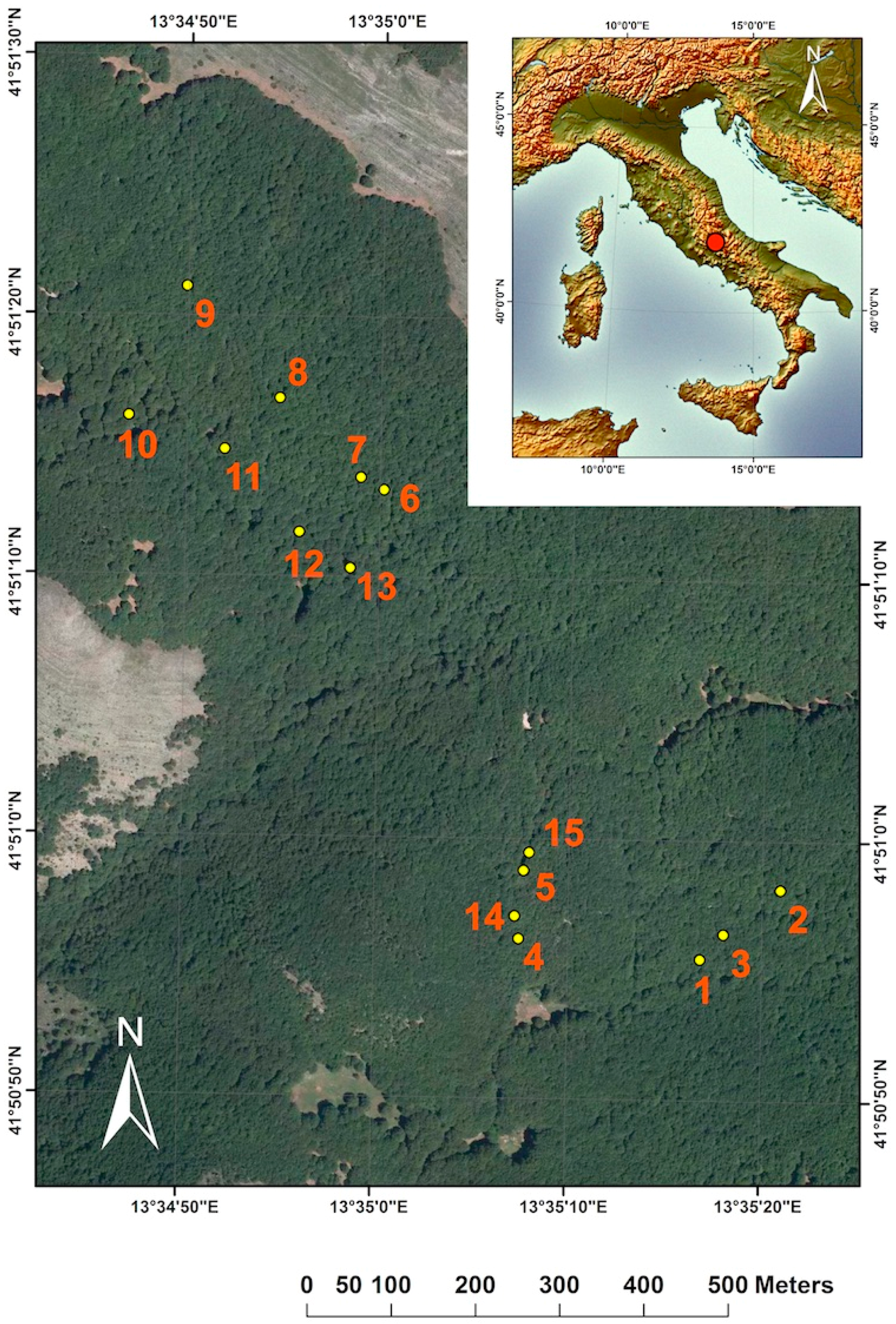
3.1. Study Site

The experiment was carried out at the Collelongo-Selva Piana pure beech forest (Abruzzo region, Central Italy, 41°50′58″N, 13°35′17″E, 1560 m elevation). The site is part of a wider forest area, included in the external belt of the Abruzzo-Lazio-Molise National Park and its structure and conditions are representative of Central Apennine beech forests [54]. The site is equipped with a 28 m scaffold tower geared towards measuring ecosystem H₂O and CO₂ fluxes using the eddy covariance technique, as previously described by other studies [55,56]. According to EUNIS (European Nature Information System) habitat classification, the site is included into the Southern Italian beech forests type. The vegetation is homogeneous and dominated by European beech (Fagus sylvatica L.) within the area of approximately 1 km × 1 km around the flux tower. The understory is sparse, patchy, and mostly formed by herbs (coverage less than 2%, height less than 50 cm). Patches of mountain prairie are observed, which introduces spatial heterogeneity typically beyond 1 × 1 km. The topography in that area is gently and variably sloped (with plain areas, hollows, and mountain sides), with elevation ranging from 1500 to 1650 m. The climate is Mediterranean montane, with cool to moderately warm summer and cold winters. The mean annual temperature and precipitation measured at the site for the period 1996–2015 are 6.9 °C and 1116 mm; soil has a variable depth ranging from 40 to 100 cm and is classified as humic soil [57]. In the area of the experimental site, plant density is 740 trees·ha⁻¹ (starting from trees with 1 cm diameter at 1.30 m), the basal area is 42.2 m²·ha⁻¹ with a mean diameter at breast height of 25.5 cm and a mean height of 20.7 m (data from the 2012 periodic five-year stand survey). At the peak of the growing season, the Leaf Area Index (LAI) in 2014–2015 was 5.5–5.9 m²·m⁻² [58]. Previous works [56,59,60] provide a detailed description of the site and of the stand structure. The Collelongo-Selva Piana experimental site is currently part of the following projects: LIFE+ Smart4Action, eLTER H2020, PRIN 2012 Nitrogen in Mediterranean Forest, and CNR IBAF Ecology and Dynamics of Forest Systems. It is also part of international networks such as LTER-Europe, Fluxnet, ICP-Forests, ICP-Integrated Monitoring, and the CONECOFOR program.

3.2. Temporal and Spatial Sampling

The study area used for satellite validation covered 5 km × 5 km and is centered at the flux tower (41°50′58″N, 13°35′17″E). Different temporal and spatial sampling was performed depending on the three different devices used in the experiment, two PAR sensors (Apogee and PASTIS; details in the following section) and digital cameras for collecting hemispherical photographs (DHP). The ground sampling was concentrated over a homogeneous area of approximately 1 km² around the flux tower, where 15 spatial units called Elementary Sampling Units (ESUs) were taken as references (Figure 1). Each ESU is approximately 20 m × 20 m and was selected to cover the variability of the site around the flux tower area. The center of each ESU was geo-located using a Global Positioning System (GPS). ESU 1 (centered at the flux tower) was selected for an intensive PAR measurement sampling for its proximity to the reference above canopy sensors and thus equipped with Apogee-PAR sensors from July to December 2014 and from May to December 2015 (

Table 3. Specifications of ground data sampling in the study.

Name of the Sensor	Spatial Sampling	Temporal Sampling	Description
Apogee-PAR	ESU 1 (tower)	July–December 2014 May–December 2015 (daily)	22 PAR sensors—Continuous measurements
PASTIS-PAR	ESUs 1–9	May–December 2015 (daily)	10 data logger with 6 PAR sensors each—Continuous measurements
Digital camera collecting Digital Hemispheric Photographs (DHPs)	ESUs 1-15	8 July 2015 25 September 2015	13 DHPs for each ESU

). ESUs 1–9 were equipped with PASTIS-PAR sensors from May to December 2015. All 15 ESUs were involved in two field campaigns on 8 July and 25 September 2015 for the spatial characterization of vegetation variables with DHPs (Figure 1). Manufacturer details are provided in Section 3.3.

3.3. Ground Measurements and Instruments

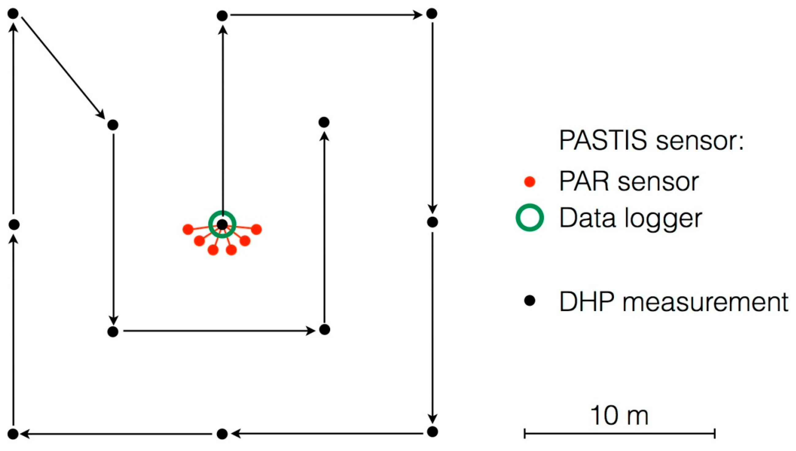
3.3.1. PAR Measurements from Apogee

Continuous PAR measurements of incident, transmitted, and reflected PAR were collected according to the protocol for PAR measurements developed within the FP7 ÉCLAIRE Project (http://www.eclaire-fp7.eu/). In total, 22 PAR sensors (SQ-110, Apogee Instruments, Logan, UT, USA) were installed around the flux tower (800 m²) [61]. Specifically, 15 sensors pointing upward were mounted below the canopy to monitor transmitted PAR through the canopy ($PA{R}_b^{\downarrow }$) and five sensors pointing downward were mounted below the canopy to monitor reflected PAR by the soil ($PA{R}_b^{\uparrow }$). At the top of the tower, two sensors were installed on a horizontal 2-m arm to measure incident PAR above the canopy ($PA{R}_a^{\downarrow }$) and reflected PAR from the canopy ($PA{R}_a^{\uparrow }$), respectively. To maximize the radiometric footprint, below-canopy PAR sensors pointing downward were installed on a 2 m high pole while below-canopy PAR sensors pointing upward were installed on a 1 m high pole. PAR measurements were acquired every 10 s and stored as 30-min averages as μmol m⁻²·s⁻¹.

3.3.2. PAR Measurements from PASTIS

At ESUs 1–9, PASTIS device (PASTIS-PAR, INRA-Hyphen, Avignon, France) were installed to continuously measure transmitted PAR through the canopy ($PA{R}_b^{\downarrow }$). In addition, one PASTIS device was also installed above the flux tower at ESU 1 to measure incident PAR radiation above the canopy ($PA{R}_a^{\downarrow }$).

Each PASTIS system consists in a data logger associated to six wired hemispherical quantum sensors measuring instantaneous PAR signal in millivolts (http://www.hiphen-plant.com/products/pastis_18.html) [62]. Below the canopy, the data logger was fixed at a labeled tree while the sensors were installed at soil level. Each of the six sensors was mounted on a 30 cm long support bar to prevent falling leaves and other litter from covering the quantum sensors while acquiring data.

PAR measurements were acquired every minute. PASTIS sensors measured downward radiation both above and below the canopy and an intercalibration against Apogee sensors was performed in order to combine Apogee and PASTIS measurements for fAPAR computation at the ESUs. Both PASTIS and Apogee PAR continuous ground measurements were used to qualitatively assess the temporal courses of the satellite products.

3.3.3. Gap Fraction Estimation from DHP

Two hemispherical digital photography (DHP) cameras were used for estimating fAPAR at the study area: CANON EOS 6D with a SIGMA 8mm F3.5–EX DG and NIKON Coolpix 995-FCE8. In order to accurately process the images, the optical center and the projection function of the optical system were calculated for each camera [63]. At each ESU, 13 DHPs were taken pointing the camera upward-looking. A measurement was acquired every 10 m along the path (black circles, Figure 2) to cover the ESU area (20 m × 20 m), in agreement with the VALERI spatial sampling protocol (http://w3.avignon.inra.fr/valeri).

DHP acquisition was processed using CAN-EYE software version 6.4 developed at EMMAH Avignon (http://www6.paca.inra.fr/can-eye) for deriving biophysical variables (LAI, fAPAR, fCOVER) from hemispherical photos. Since CAN-EYE is based on a RGB color classification of the image to discriminate vegetation elements from the background (i.e., gaps), photos were acquired with similar illumination conditions to limit the variation of color dynamics between images. DHPs processing consisted of three steps: (1) image pre-processing aimed to remove undesired objects (e.g., operator, sun glint) and ensure better visual discrimination between vegetation and background adjusting image contrast; (2) assignment of the colors to each class (vegetation elements versus background) after reducing the number of distinctive colors in order to easily manipulate the image; and (3) realization of a binary image (background versus vegetation elements), using the classification results [64].

3.4. Calculation of Ground Canopy fAPAR

3.4.1. Estimation of fAPAR from Apogee (fAPAR_APOGEE)

In this work, the Apogee sensors, given the set-up, the spatial coverage, and the measurements of all fAPAR components (see Section 3.3.1), provided the reference fAPAR value at the tower site (ESU 1) against which PASTIS and DHP measurements were compared. Having the four PAR contributions, fAPAR from Apogee measurements (fAPAR_APOGEE) was calculated as reported by Liang et al. [65]:

$$fAPAR=\frac{PA{R}_a^{\downarrow }-PA{R}_b^{\downarrow }-PA{R}_a^{\uparrow }+PA{R}_b^{\uparrow }}{PA{R}_a^{\downarrow }},$$

(1)

where $PA{R}_a^{\downarrow }$ is the incident PAR above the canopy, $PA{R}_a^{\uparrow }$ is the reflected PAR above the canopy, $PA{R}_b^{\downarrow }$ is the transmitted PAR through the canopy, and $PA{R}_b^{\uparrow }$ is the reflected PAR by the soil [65]; all components are hemispherical quantities. As temporal mismatching between in situ data and satellite observation could be critical [66], we calculated fAPAR as averages from 10:00 a.m. to 11 a.m. to guarantee temporal matching between ground data and the satellites overpass. For the purpose of validating fAPAR products, only photosynthesizing materials (leaves, needles, or other green elements) should be accounted for in the calculation (green fAPAR) [41]. Nevertheless, in homogeneous deciduous forests where LAI reaches maximum values that remain stable during the vegetative season, the influence of non-photosynthetically active vegetation (NPV) elements (such as trunks and branches) in the fraction of absorbed PAR by the canopy is expected to be quite small as compared to the green elements. For instance, Zhang et al. [67] showed that in the Harvard deciduous forest the contribution of NPV to the fAPAR is lower than 0.1 in spring and summer time, whereas the fAPAR from green elements reaches 0.85 in summer time. In line with this work, we assume that the largest impact of NPV elements in our ground dataset occurred during the senescent period.

3.4.2. Estimation of fAPAR from PASTIS (fAPAR_PASTIS)

fAPAR_PASTIS was computed using two sets of measurements in Equation (1): incident and reflected PAR obtained from Apogee and transmitted PAR obtained from PASTIS (previously intercalibrated, as reported in Section 3.3.2). The adapted equation was computed as follows:

$$fAPA{R}_{PASTIS}=\frac{PA{R}_{a APOGEE}^{\downarrow }-PA{R}_{b PASTIS}^{\downarrow }-PA{R}_{a APOGEE}^{\uparrow }+PA{R}_{b APOGEE}^{\uparrow }}{PA{R}_{a APOGEE}^{\downarrow }},$$

(2)

We used the same method to calculate $fAPA{R}_{PASTIS}$ at each of the nine ESUs equipped with PASTIS sensors. It is worth noting that incident $PA{R}_{aPASTIS}^{\downarrow }$ was not used in Equation (2) since a long data gap occurred due to battery loss. $fAPA{R}_{PASTIS-ESU n}$ stands for fAPAR computed at ESU_n, while $fAPA{R}_{PASTIS-AVG}$ stands for fAPAR computed averaging transmitted PAR ($PA{R}_b^{\downarrow }$) of ESUs 1–9.

3.4.3. Estimation of fAPAR from DHPs

Among other measurements related to canopy architecture (e.g., LAI), hemispherical photos allow the computation of fAPAR by measuring the directional gap fraction [64,68]. In fact, as the photosynthetically active radiation domain (PAR, 400–700 nm) is characterized by strong absorbing features of the photosynthetic pigments [69], fAPAR is often assumed to be equal to fIPAR (Fraction of Intercepted Photosynthetically Active Radiation) [26], and therefore is directly related to the gap fraction. According to this assumption, CAN-EYE software proposes three outputs for fAPAR: the instantaneous black-sky (or direct) fAPAR; the daily integrated black-sky fAPAR and the white-sky (or diffuse) fAPAR. In our study, we selected the instantaneous black-sky fAPAR at 10:00 a.m. ($fAPA{R}_{10h}^{BS}$) for consistency with satellite products and we refer to it as fAPAR_DHP. According to CAN-EYE output variable description [70], fAPAR_DHP was computed using the following Equation (3):

$$fAPA{R}_{DHP}=fAPA{R}_{10h}^{BS}={1-P_0({\theta }_S)|}_{S=10h},$$

(3)

where $P_0$ represents the measured gap fraction on each viewing zenith angle $\theta$ and ${\theta }_S$ is the sun zenith angle at 10:00 local solar time [70].

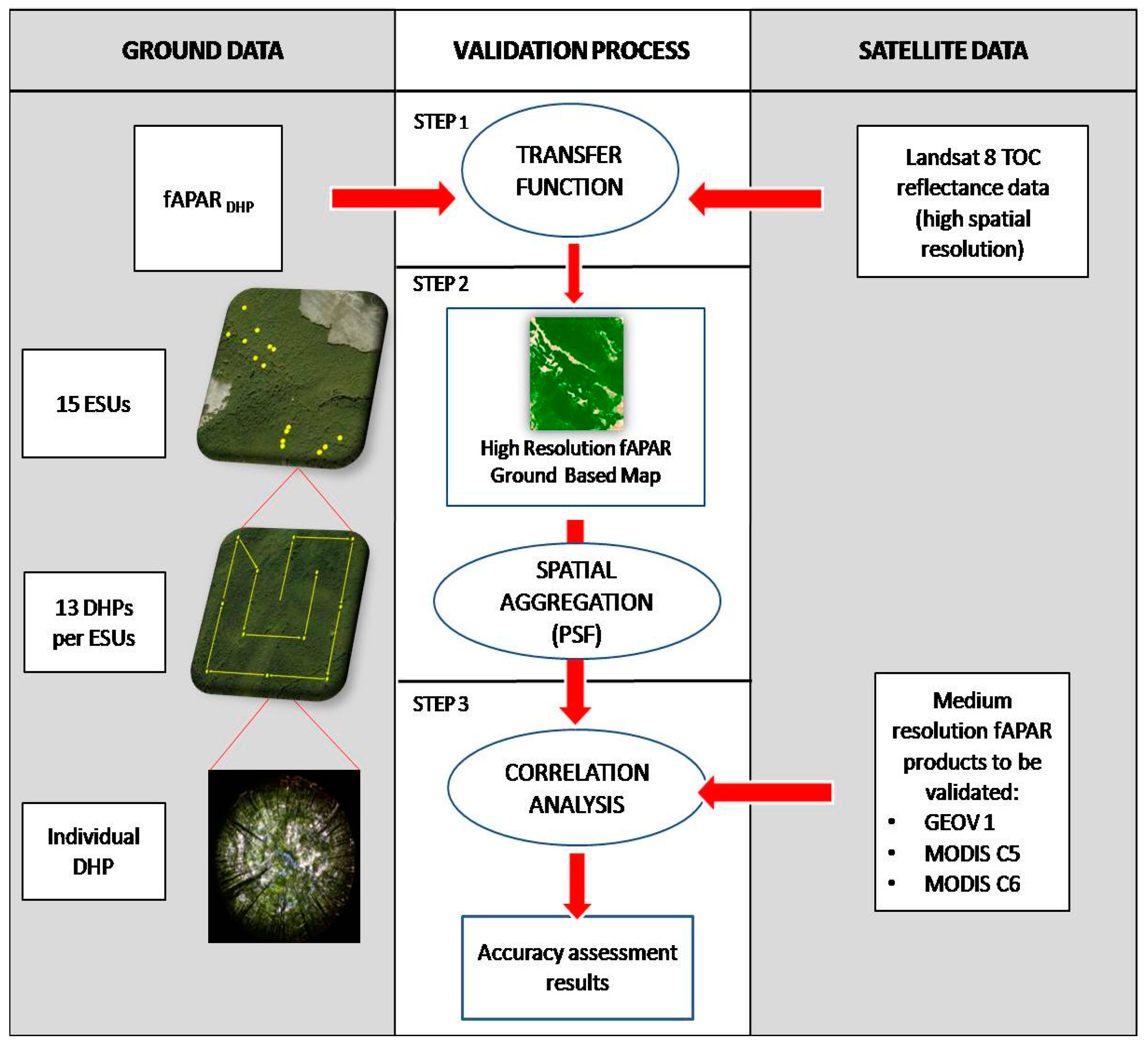
3.5. Validation Approach

To perform a direct validation of medium-resolution satellite products, we need to account for the differences in scale between the footprints of the ground measurements and the satellite sensor. For this reason we followed the bottom-up approach proposed by the CEOS LPV sub-group summarized in Figure 3. This approach consists of using high-resolution imagery and robust regression methods to upscale the ground measurements from ESU values to the site level. The resulting ground-based map can then be aggregated to the spatial resolution of the satellite product to be validated. The first step was deriving an empirical transfer function (TF) that establishes a relationship between the canopy fAPAR_DHP values (the only measurement available at all 15 ESUs), plus additional control values obtained in prairie and over bare areas, and the multispectral radiometric values from the high-resolution Landsat-8 imagery [71] (Section 3.5.1). The ground-based high-resolution maps, derived from the selected transfer function, were then remapped to the spatial support of GEOV1 and MODIS products (i.e., 1 km and 500 m), taking into account the equivalent Point Spread Function (PSF) of the satellite sensors [43] (Section 3.5.2). Then, the aggregated maps of canopy fAPAR were compared to the moderate-resolution green fAPAR satellite products under the assumption that canopy fAPAR is very close (differences lower than 10%) to green fAPAR during the peak season. Finally, validation statistics were computed for the accuracy assessment (Section 3.5.3).

3.5.1. Empirical Transfer Function

For the up-scaling of the ground measurements at the site level, we need to establish an empirical relationship (transfer function) between the canopy fAPAR ground values and concomitant radiometric values of a high-resolution imagery. For this purpose, Landsat-8 top-of the canopy reflectance images of 30 m spatial resolution were selected. Landsat-8 images are freely available at the USGS earth explorer portal (http://earthexplorer.usgs.gov/). The acquisition date was 10 July and 27 August 2015, for the first and second campaign, respectively. For the second campaign, the date of acquisition is around one month earlier than the ground sampling, due to cloud contamination of concomitant Landsat-8 acquisitions for the September campaign. However, as ground measurements showed high stability from July to the end of September, we also assumed stability in the radiometric signal of the image during this period.

A multivariate ordinary least square (OLS) regression was used for modeling the relationship between fAPAR_DHP (our response variable) at the ESU level and the radiometric information of the Landsat-8 image (predictor variable) [71]. The multivariate OLS function proposed in this work uses an iteratively re-weighted least squares (IRLS) algorithm in order to minimize the influence of outliers as proposed by Martinez et al. [71]. This method allows for combining the information provided by different bands and evaluating the band combination that exhibits the lowest error. This modeling approach has been recently used for upscaling biophysical variables such as LAI, fAPAR and fCOVER over a network of cropland sites in the ImagineS project (fp7-imagines.eu/). The basis is that outliers in the sampling distribution will result in biased estimates of model parameters. The IRLS algorithm includes an additional scale factor (i.e., weight) in order to adjust the amount of influence each response value has on the model estimates [71]. The following bands were considered: B3 (green: 0.53–0.59 µm), B4 (red: 0.64–0.67 µm), B5 (NIR: 0.85–0.88 µm), B6 (SWIR1: 1.58–1.65 µm). Due to the well-known linear or approximately linear relationship between fAPAR and NDVI [19,72,73,74,75,76], we also used B4 and B5 to compute NDVI [77] and additionally use it as a predictor variable (Equation (4)). In addition to the ESU measurements over the forest, additional values over bare areas and prairie were used to better constrain the model for low fAPAR values. Control points included four bare areas that were visually selected with GoogleEarth^® around the study area, with NDVI ranging between 0.06 and 0.17, and where fAPAR was set to 0. Furthermore, an additional ESU located over a prairie area with DHP measurement was used to calibrate the empirical transfer function in order to have intermediate values of fAPAR. The obtained value with CAN-EYE for the black-sky fAPAR at 10 h over the prairie ESU was 0.73.

In order to assess the model performance and evaluate the optimal predictor three different errors were computed: the root mean square error (RMSE), the weighted RMSE (RW, using the weights attributed to each ESU) and the cross-validation RMSE (RC, leave-one-out method). RMSE and RW provides an estimate of the mean prediction error of the model considering all the observations, whereas RC provides a more reliable model performance since it gives an indication of how well the function will predict data not included in the data set used to derive the predictor [78]. The NDVI was chosen as input for the transfer function because it shows lower RC errors than other band combinations for the first, the second and the combined campaigns [79].

Table 4. Performance metrics of empirical transfer function. Positive bias indicates overestimation of the transfer function estimates. RC stands for cross-validated RMSE; RW stands for weighted RMSE.

Field Campaigns	R2	Bias	RMSE	RC	RW
8 July 2015	0.999	−0.001	0.015	0.018	0.015
25 September 2015	0.995	−0.009	0.041	0.063	0.062
Both campaigns	0.995	−0.003	0.03	0.049	0.025

shows the errors (RMSE, RW, RC) obtained for the selected transfer function using the NDVI for the first and the second campaign, as well as when the data of the two campaigns were pooled together. It can be noticed that all the different cases show very low RMSE errors, below GCOS requirement on accuracy [44], and very high correlation coefficients (>0.99) with almost no mean bias (Table 4). The higher errors obtained for the second campaign could be partly attributed to the period between the collection of ground measurements (end of September) and the imagery acquisition (end of August). Finally, we selected the transfer function based on the two ground campaigns in order to reduce errors of the second campaign, with a final cross-validation RMSE of 0.049.

The empirical relationship selected for our site is the following linear relationship based on NDVI computed from Landsat red (B4) and NIR (B5) bands:

$$fAPAR=-0.1799+1.2258\times \left(\frac{{\rho }_{NIR}-{\rho }_{red}}{{\rho }_{NIR}+{\rho }_{red}}\right)$$

(4)

where ${\rho }_{NIR}$ and ${\rho }_{red}$ is the reflectance in the near infrared and red, respectively.

The high-resolution ground-based maps over the site are shown in Section 4.2.

Finally, the convex hull technique described by Martinez et al. [71] was applied to characterize the representativeness of ESUs and the reliability of the empirical transfer function. This technique will allow us to derive a quality assessment image to highlight areas on the fAPAR maps with higher or lower confidence of the estimates due to the model errors and sampling strategy. Briefly, this method defines a convex region delimited by the data set containing the spectral information of the in-situ measurements and can be applied using multiple spectral bands combinations in agreement with our multivariate OLS approach for selecting the optimal band combination for the transfer function. This region delimits the domain where the transfer function behaves as interpolator (namely ‘strict convex hull’). Conversely, outside this domain, the transfer function behaves as extrapolator. However, the convex hull could be slightly expanded by ±5% of reflectance (namely ‘large convex hull’) to allow pixels very close to the strict convex hull to be used since they are expected to provide reasonable results. Hence, this test was carried out using the red (B4) and NIR (B5) bands of the Landsat-8 images used for the NDVI computation. In this case the hull is an area on the red-NIR plane, the spatial distribution for each of the three regions defined is provided in the quality flag images presented in Section 4.2.

3.5.2. Spatial Aggregation

The comparison between the ground-based maps with moderate-resolution products requires a consistent statistical support area. This apparently simple problem should be considered carefully if all uncertainties associated to satellite products are to be recognized [43]. Firstly, the satellite products and the high-resolution maps were projected to the same coordinate system. The Plate Carrée projection of GEOV1 product was used for the comparison at both 1 km and 500 m. A spatial window of 5 km × 5 km centered over the tower was selected for the comparison. Secondly, the high-resolution map was aggregated to the spatial resolution of the satellite product according to the effective point spread function (PSF) of the satellite product, which improves the performance of the evaluation as compared to ordinary average [80]. The equivalent PSF results from a number of steps that need to be considered. The instrument PSF depends on several components: the electronic PSF, the detector PSF, the image motion PSF, and the optical PSF [81]. According to Duveiller et al. [82], electronic and image motion PSFs can be neglected. The PSF for the MODIS and PROBA-V instruments can be approximated by the convolution of a Gaussian function characterizing the optical PSF. The ground-based map equivalent PSF was computed by maximizing the correlation coefficient between the low-resolution (LR) product (i.e., GEOV1, MODIS C5 and C6) and the corresponding higher resolution (HR) image. During the optimization process of the PSF, we used an iterative approach in which we combined the extension of the pixel size and the PSF characterized by the Full Width at Maximum (FWHM) of the two Gaussian functions in both the x and y directions. The extension of the pixel was combined in steps of 30 m (HR) up to the pixel size of the corresponding LR product.

3.5.3. Correlation Analysis

The accuracy assessment between the ground-based maps and the satellite products to be validated was performed at the resolution of the satellite product to evaluate on a pixel by pixel basis. The comparison was performed using the closest product date to the field campaign. The accuracy was quantified by several validation metrics reporting the goodness of fit between the products. Total measurement uncertainty (i.e., root mean square error, RMSE) includes systematic measurement error (i.e., bias) and random measurement error (i.e., standard deviation of bias). RMSE corresponds to the accuracy as there is only one product estimate for each mapping unit [83]. RMSE is recommended as the overall performance statistic. Linear model fits were also used to quantify the goodness of fit. For this purpose, Major Axis Regression (MAR) was computed instead of OLS because it is specifically formulated to handle error in both the x and y variables [84]. Finally, the number of pixels within the GCOS requirements was quantified.

Table 5. Uncertainty metrics for product validation.

Gaussian Statistics	Comment
N: Number of samples	Indicative of the power of the validation
RMSE: Root Mean Square Error	Indicates the Accuracy (Total Error)
	Relative values between the average of x and y were also computed
B: Mean Bias	Mean difference between pair of values (y–x)
	Indicative of accuracy and possible offset
	Relative values between the average of x and y were also computed
S: Standard deviation	Indicates precision
R2: Correlation coefficient.	Indicates descriptive power of the linear accuracy test
	Pearson coefficient was used
Major Axis Regression (slope, offset)	Indicates possible bias
% GCOS requirements	Percentage of pixels matching the GCOS requirements

summarizes the uncertainty metrics associated with the scatter-plots.

4. Results

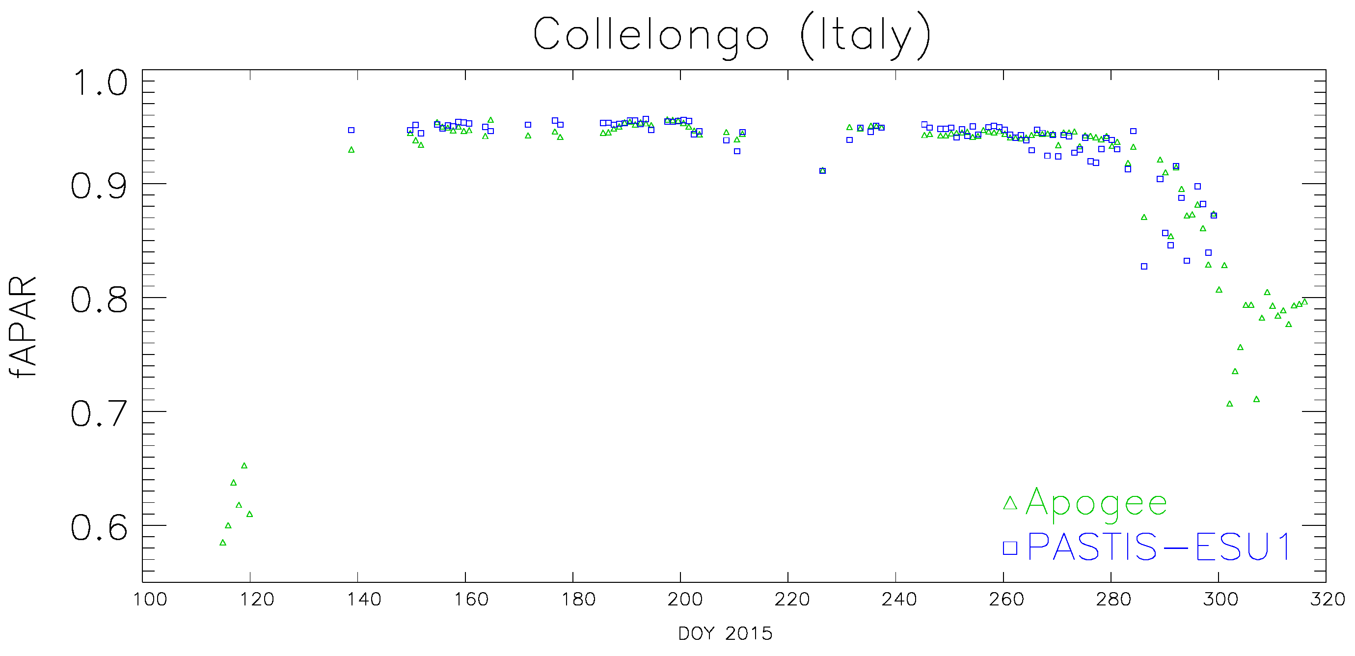
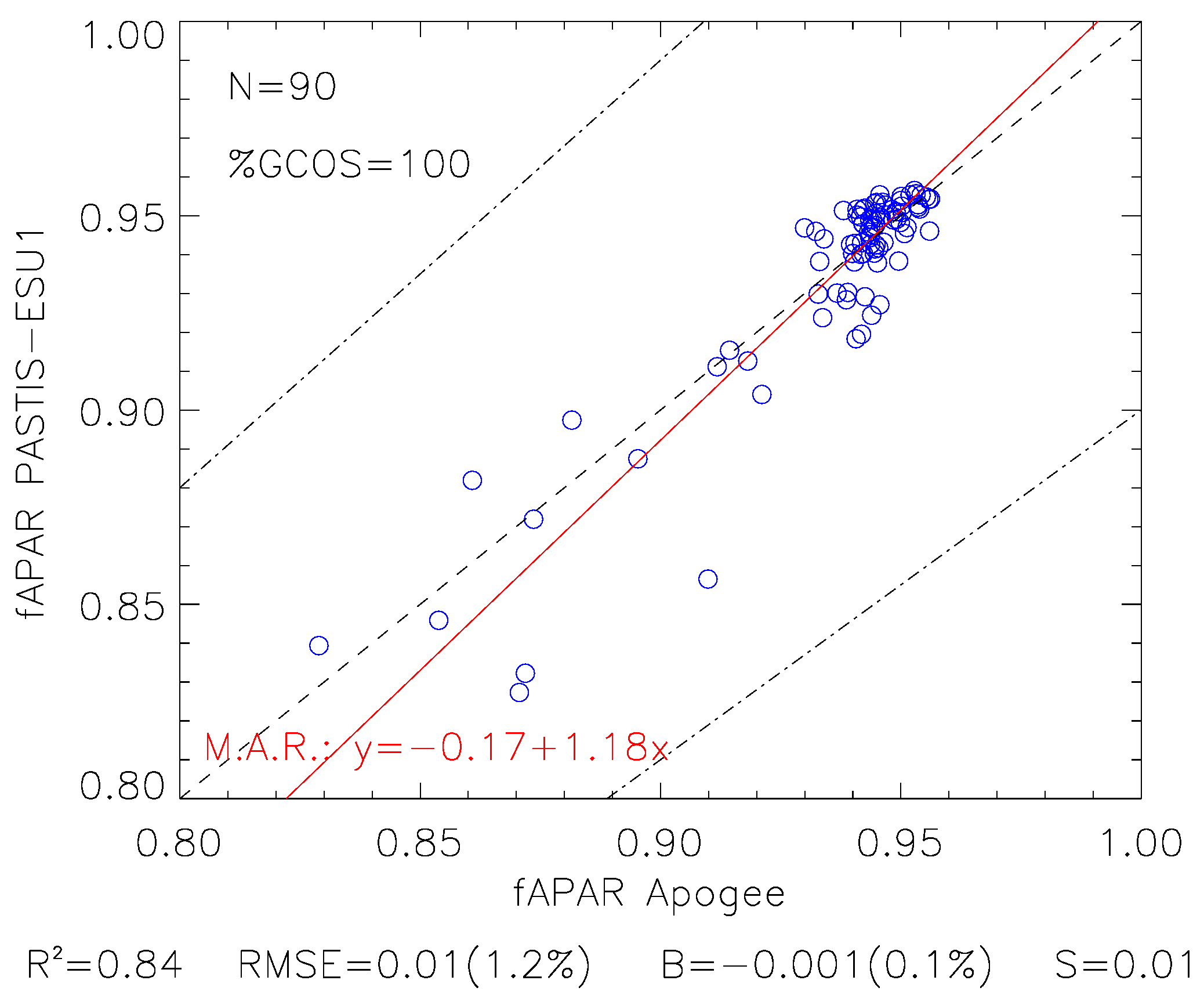
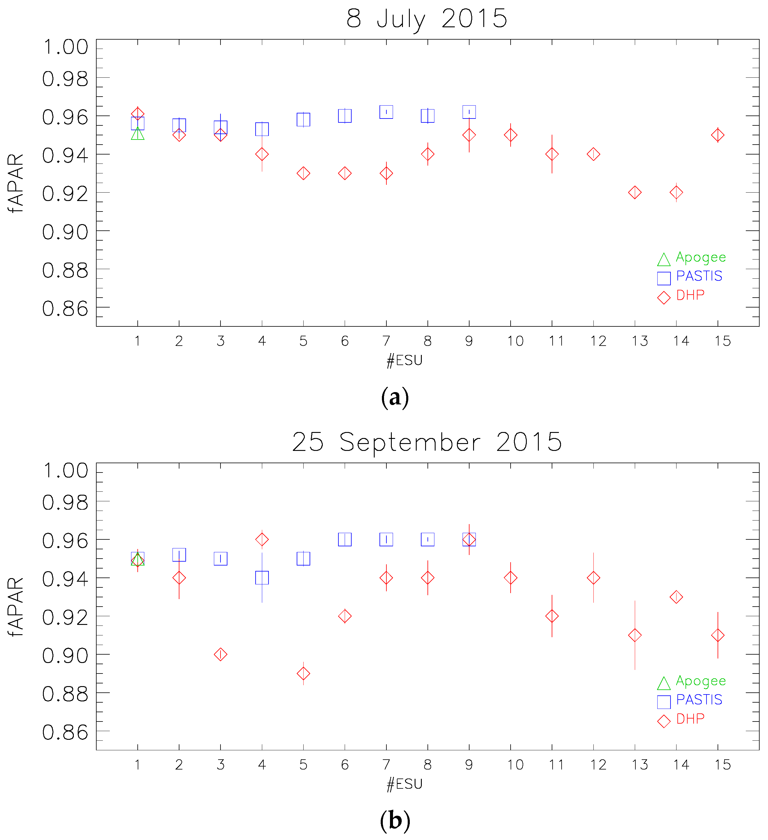
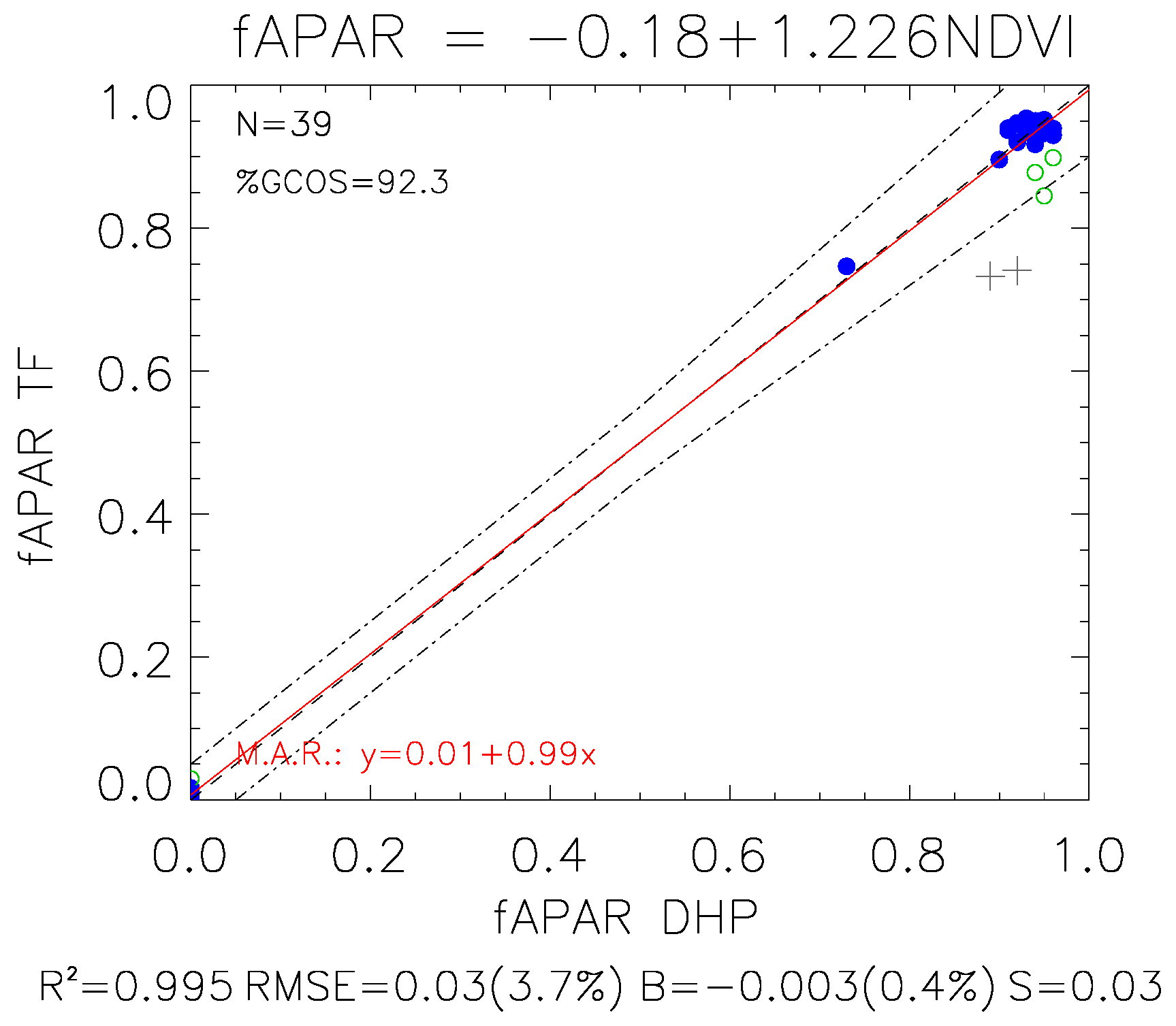
4.1. Consistency of Ground fAPAR Estimates

We investigated the temporal course of PASTIS sensors by comparing fAPAR_PASTIS-ESU1 with fAPAR_APOGEE at ESU1 during 2015. Figure 4 shows synchronism between fAPAR_APOGEE, which represented our benchmark, and fAPAR_PASTIS-ESU1. At the end of April (DOY 110–120), fAPAR_APOGEE values ranged between 0.55 and 0.65. Starting from the last ten days of May (DOY 139), until the first ten days of October (DOY 283), fAPAR_APOGEE presented fairly constant values of 0.93–0.96 during the whole period. During this phase, both the average of fAPAR_APOGEE and fAPAR_PASTIS was 0.94, with a standard deviation (σ) of 0.007 for fAPAR_APOGEE and 0.010 for fAPAR_PASTIS. The longest gap in our dataset occurred from DOY 210 to 230, when values were presumably stable, as included in the peak season. fAPAR_APOGEE values started to decline in mid-October, decreasing steadily until the end of the year, except for the first two weeks of November, when values appeared constant around 0.78–0.79. While the evolution between fAPAR_APOGEE and fAPAR_PASTIS was in agreement during the peak season, both fAPAR values fluctuated more evidently during the senescence phase (DOY 266–280). Peak value detected by both techniques was 0.96 associated to DOY 198 for Apogee sensors and to DOY 194 for PASTIS sensors. fAPAR values measured with PASTIS sensors strongly correlated with those measured with Apogee sensor (R² = 0.84; RMSE = 0.01), although a bigger fluctuation was observed in the senescence phase (fAPAR < 0.9, Figure 5), as formerly evidenced by the seasonal patterns (Figure 4).

Data from PASTIS and DHP sensors at the different ESUs were compared for the two DHP sampling campaigns. fAPAR_DHP ranged from 0.92 to 0.96 for the campaign in July, while fAPAR_PASTIS presented values between 0.95 and 0.96 (Figure 6a). Generally, fAPAR_PASTIS was higher than fAPAR_DHP and in agreement with it, except for ESU 5–8. During September campaign, fAPAR_DHP resulted generally lower than fAPAR_PASTIS (Figure 6b). While fAPAR_PASTIS varied between 0.94 and 0.96, fAPAR_DHP spanned from 0.89 to 0.96. Analyzing the standard deviation (error bars) of the measurements, it appeared that fAPAR_PASTIS had less variability among the single replicates compared to fAPAR_DHP during both campaigns (Figure 6). Nevertheless, fAPAR estimated from DHP based on gap fraction was consistent with fAPAR_PASTIS within the range of accuracy required for satellite products (max[5%, 10%]).

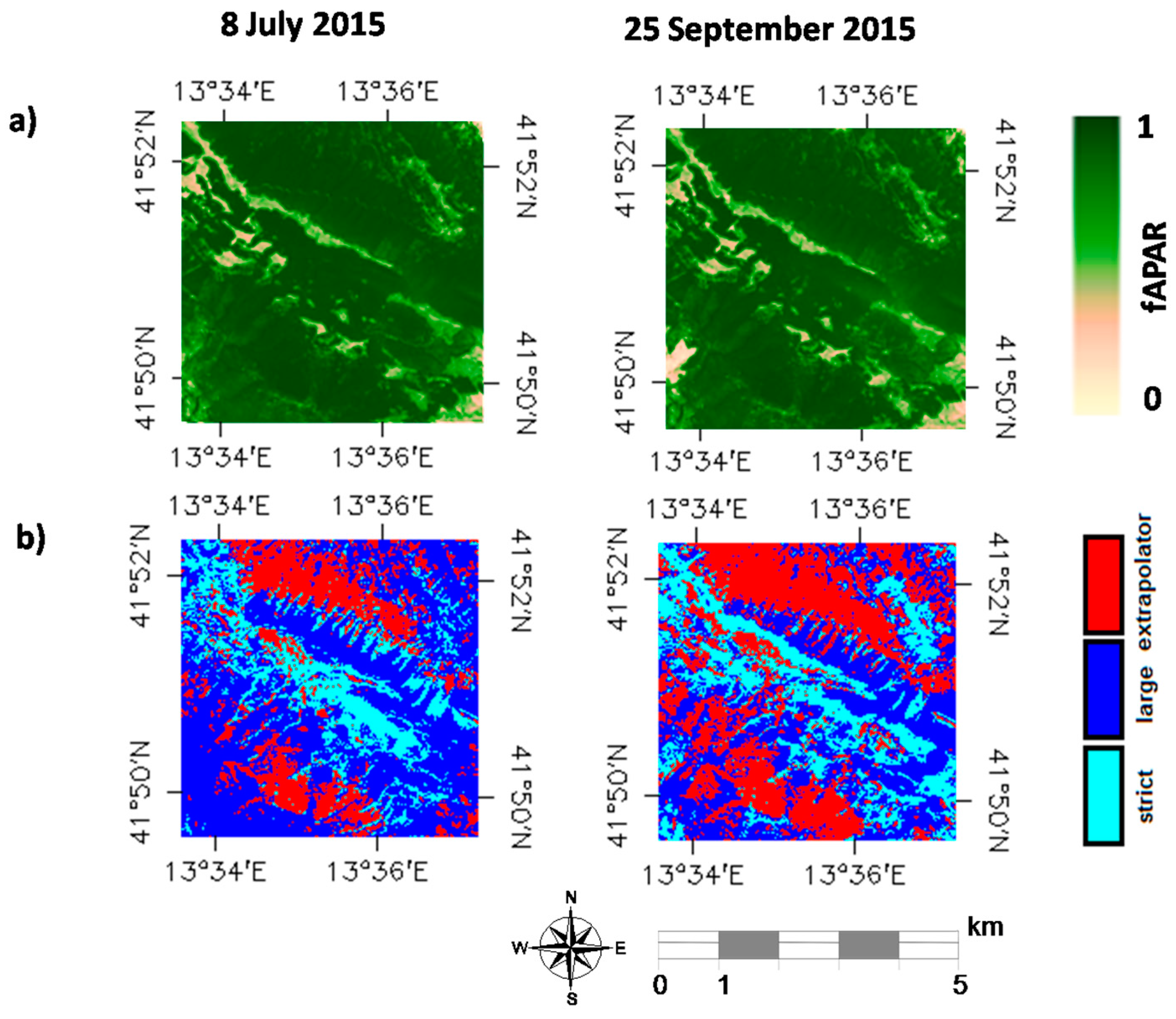
4.2. High-Resolution Ground-Based Maps

High-resolution ground-based fAPAR maps were computed with a single transfer function for both dates (Equation (4)). Figure 7a shows the spatial distribution of the retrievals over the study area, which displayed homogeneous areas of dense vegetation with high fAPAR values and some patches of low photosynthetic activity that correspond to montane prairie and/or bare rock/soil areas. Mean fAPAR value over 3-km × 3-km centered at the tower was 0.85 (σ = 0.13) for the July campaign and 0.85 (σ = 0.14) for the September campaign. The scatter-plot between ground observations (DHP) and the corresponding transfer function estimate showed the good agreement achieved (RMSE = 0.03) with a slight over-estimation for bare areas’ control points of less than 0.05 units, and some scattering for ESUs in the second campaign (Figure 8). The only ESU over prairie shows good agreement very close to the 1:1 line. The stability of fAPAR values between July and September was supported by net ecosystem exchange (NEE) values, which also presented a limited difference between the two dates (NEE between 10 a.m. and 11 a.m. equal to −16.9 and −14.1 for 8 July and 25 September 2015, respectively).

The quality assessment images (Figure 7b) derived from the convex hull technique are informative of the reliability of the estimates, showing higher reliability for those pixels inside of the ‘strict’ (in clear blue) and ‘large’ (in dark blue) convex hull. Blue pixels are mainly located around the tower site where the sampling was performed. The ‘strict’ and ‘large’ convex-hulls reached 79% and 65% of the pixels for the first and second field campaign, respectively. There is a quite consistent red area at the top and the bottom of the image that corresponds to the pixels where the transfer function behaves as extrapolator. This red area corresponds to areas with different topography or to montane prairie areas which were not included in our spatial sampling scheme. Note that the convex-hull test provides information on the representativeness of the sampling, but does not necessarily imply poor extrapolation capabilities of the transfer function, mainly on the same land cover type.

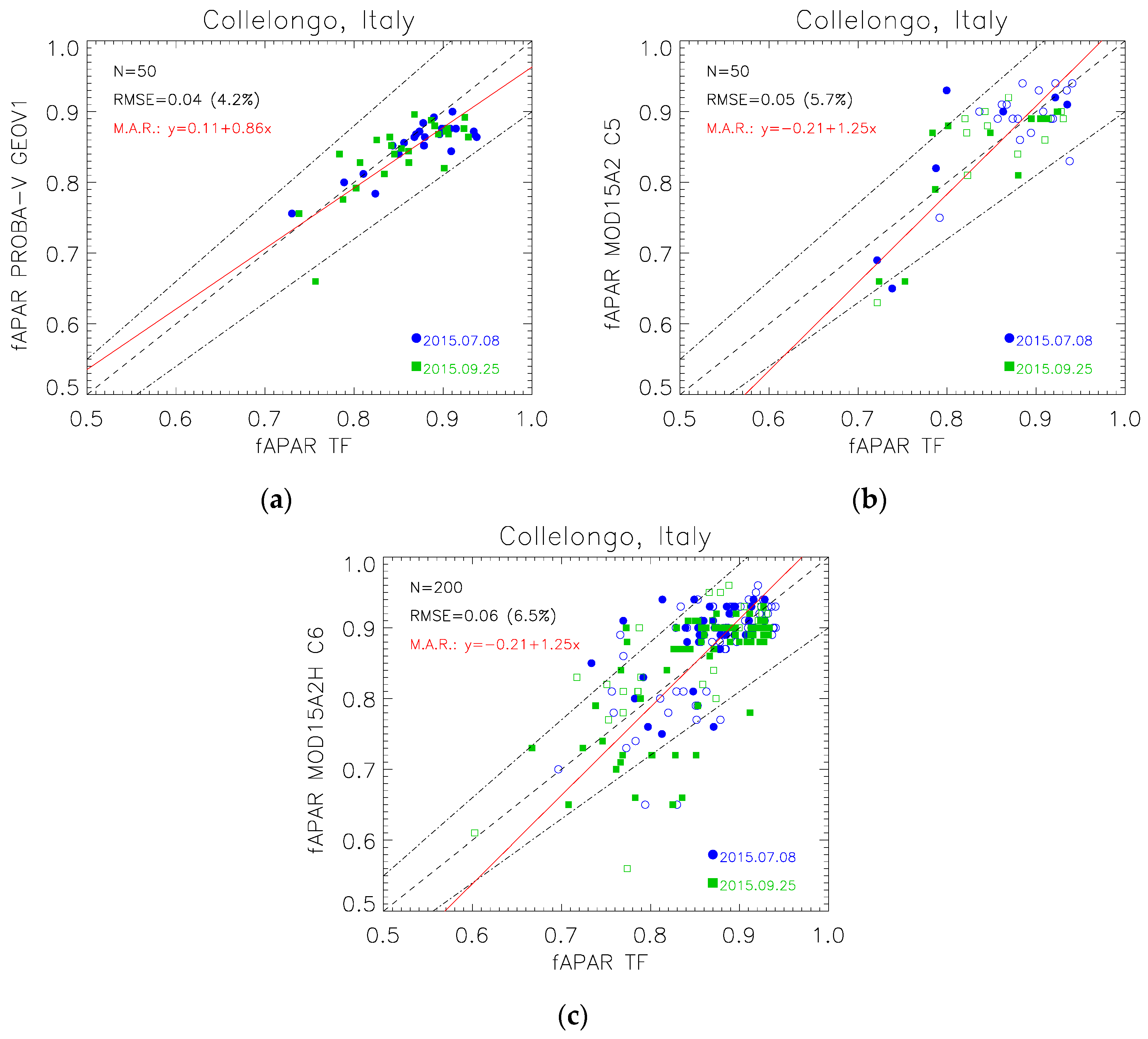
4.3. Validation of Satellite fAPAR Products

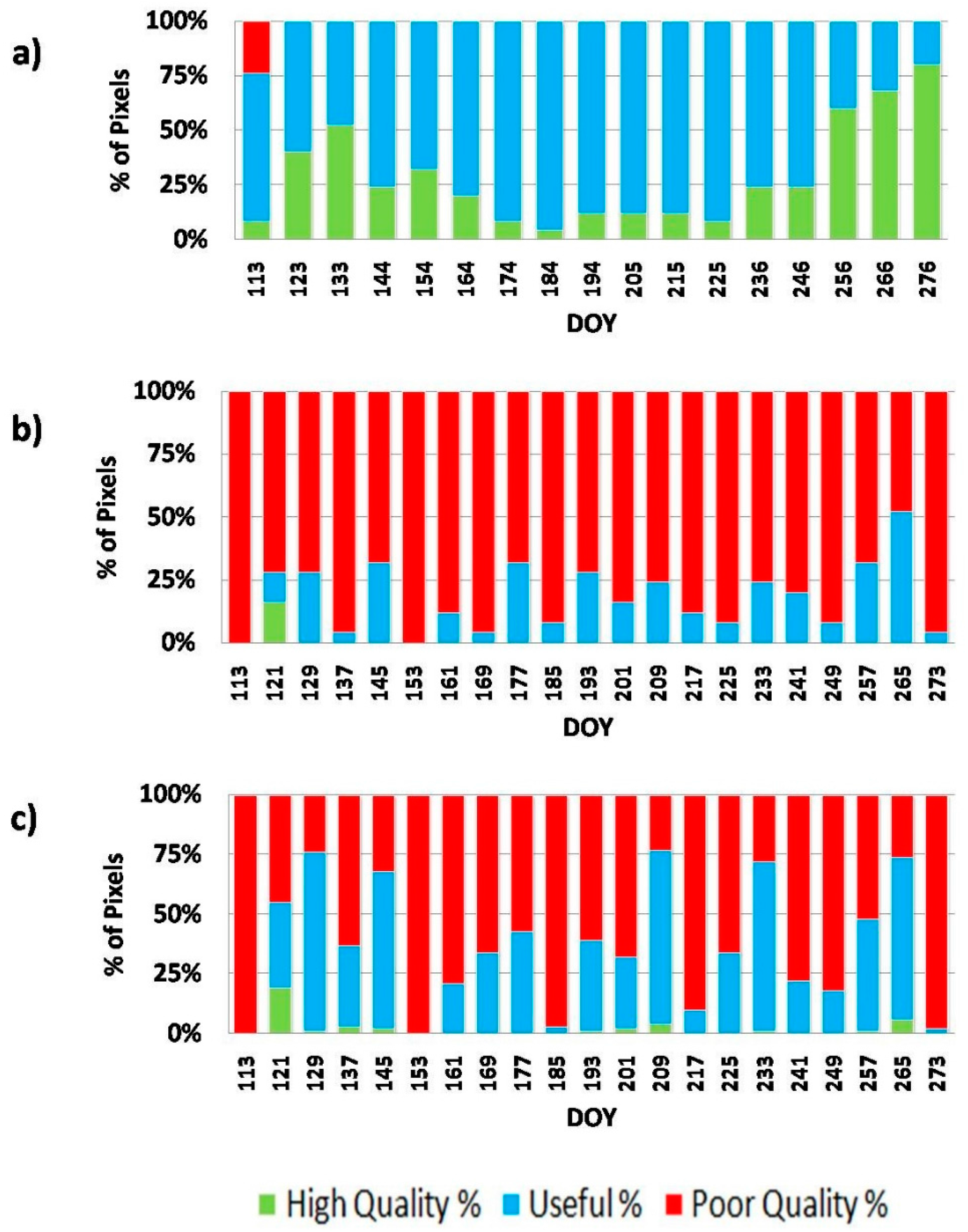
4.3.1. Product Quality Flag Analysis

We investigated the temporal courses of the QF information of GEOV1, MODIS C5, and MODIS C6 (Table 2) averaged over the 5 km × 5 km study area during the peak season (DOYs 113–276) in 2015.

During the peak season for fAPAR GEOV1 product (Figure 9a), the number of ‘high quality’ pixels was highly variable, with values falling between 8% (DOY = 184) and 80% (DOY = 276). Considering also the ‘useful’ level of quality, the percentage achieved 100% for the whole peak season except for the first date (DOY = 113) with 24% of pixels classified as ‘Poor quality’. Note that in this case where GEOV1 classifies ‘Poor Quality’ pixels, no valid or filled data was provided for the products.

On the other hand, for MODIS (C5 and C6) products, the ‘high’-quality pixels correspond to ‘Main algorithm’ and pixels free of snow, clouds, shadow and cirrus. The ‘useful’ level of quality considers the ‘Backup algorithm’ with non-contaminated input data whereas the ‘poor quality’ considers ‘Backup algorithm’ with contaminated input data. In only a few cases MODIS C5 (Figure 9b) and C6 (Figure 9c) provided the highest level of quality corresponding to main algorithm retrievals. The reason for triggering the backup algorithm is not specified in the quality flag. A larger fraction of pixels was classified as ‘Useful’ in MODIS C6 as compared to C5. This can be explained by the most precise resolution of the former, which is more accurate in detecting small clouds or shadows. Note that both MODIS versions did not present gaps over this area of 5 km × 5 km during the peak season, providing retrievals within the valid fAPAR range.

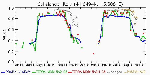
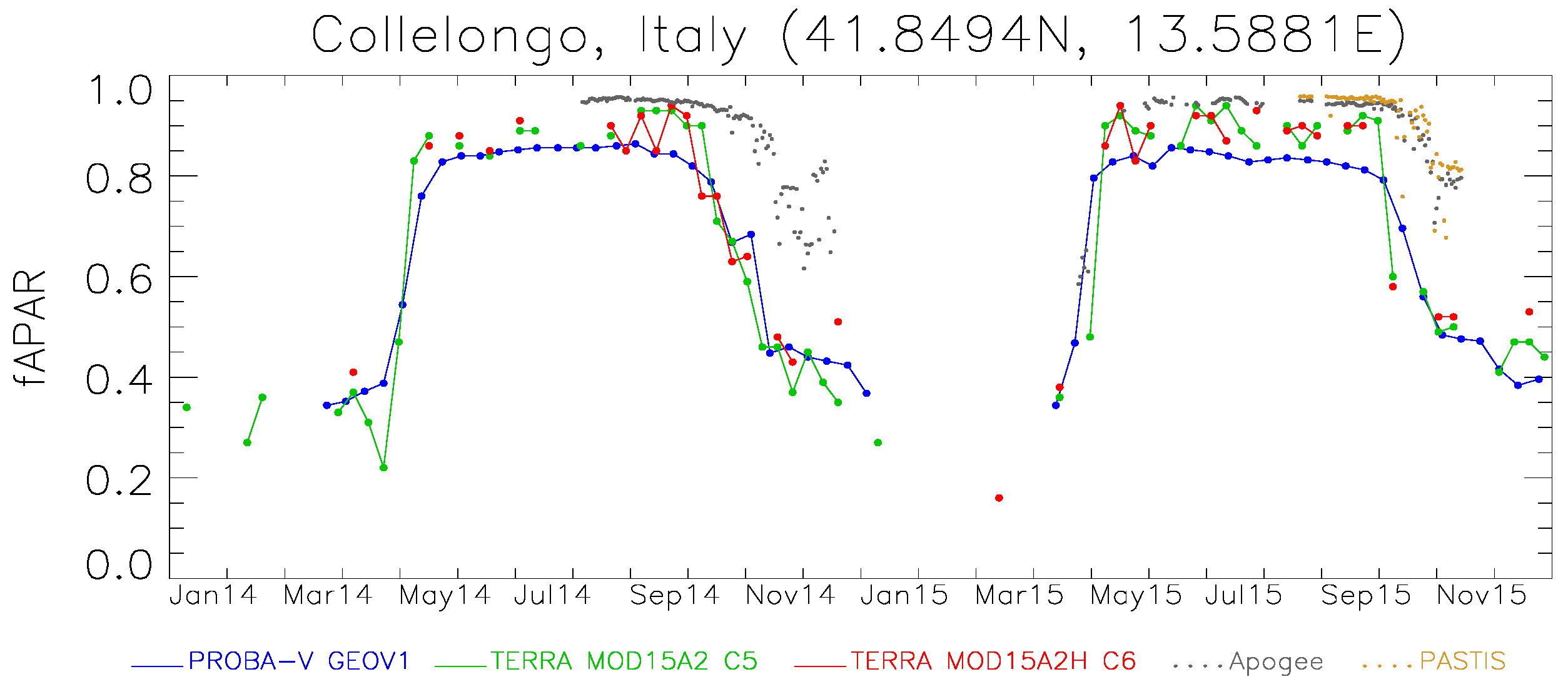
4.3.2. Temporal Consistency

The temporal variations of the three satellite products under study was evaluated over ESU 1, located at the Collelongo flux tower, where continuous fAPAR measurements were acquired (Figure 10) during the 2014–2015 period. Figure 10 displayed ground and satellite acquisitions at daily temporal frequency during the stable season (from the end of May till the end of September) and during the vegetation decrease season (from early October onwards). The initial phase of the growing season was not captured by ground measurements in either of the two years.

During the stable vegetative season, PROBA-V GEOV1 fAPAR product provided very stable temporal trajectories, in line with ground acquisitions. Regarding the magnitude of the satellite retrievals negative bias (PROBA-V GEOV1 green fAPAR < ground canopy fAPAR) was observed, that could be partly explained due to the different definition between satellite (green) and ground (total) fAPAR. The observed differences (about 0.1 units) are similar to the contribution of NPV elements to the canopy fAPAR reported by Zhang et al. [67] at the Harvard forest in summer. However, other uncertainties are present and these discrepancies may be partly attributed to the different footprints of satellite pixel (1 km) as compared to ground data (observations at the station level). Regarding both MODIS fAPAR products, similar magnitude to ground total fAPAR during the peak season were found. In line with previous studies [32,39], noisy temporal retrievals were found for MODIS products over forest areas, with variations of ±0.1 fAPAR units.

4.3.3. Accuracy Assessment

Figure 11 shows the scatter-plots between different satellite products and ground-based high-resolution maps. The validation metrics are provided in

Table 6. Performance metrics of each green fAPAR satellite product versus ground-based canopy fAPAR maps. For RMSE and Bias (negative value means underestimation of the satellite product and vice versa), the relative values are displayed in brackets.

	PROBA-V GEOV1	MODIS C5 (All Points)	MODIS C5 (High Quality and Useful)	MODIS C6 (All Points)	MODIS C6 (High Quality and Useful)
N	50	50	20	200	113
RMSE	0.04 (4.2%)	0.05 (5.7%)	0.06 (6.7%)	0.06 (6.5%)	0.06 (6.5%)
R2	0.63	0.6	0.63	0.46	0.41
Bias	−0.02 (2.6%)	−0.001 (0.2%)	0.005 (0.6%)	0.003 (0.3%)	0.003 (0.3%)
S	0.03	0.05	0.06	0.06	0.06
Offset (MAR)	0.011	−0.21	−0.23	−0.21	−0.23
Slope (MAR)	0.86	1.25	1.26	1.25	1.25
% GCOS	98	90	85	88	88

considering all data points or only high-quality and useful pixels.

PROBA-V GEOV1 green fAPAR product showed the lowest RMSE of 0.04 with low negative bias (−2.6%) mostly observed for the highest values regarding canopy fAPAR data. Almost all the points (98%) lay within the GCOS requirements on accuracy (dashed lines in Figure 11). On the other hand, similar accuracy was obtained for MODIS C5 and C6 products, with RMSE of 0.05 and 0.06 respectively, considering all pixels, almost no mean bias, and a percentage of pixels within the GCOS requirements of 90% and 88%, respectively. The slightly lower accuracy was expected due to the lower precision (i.e., higher fluctuations) previously observed in MODIS products. The finer spatial resolution of MODIS C6 (500 m) as compared to MODIS C5 (1 km) had only a minor impact on accuracy. In terms of the major axis regression (MAR) lineal model, GEOV1 product has slight better performance as compared to MODIS C5 and C6, with low offset and slope closer to 1. MODIS C6 and C5 provides good match for highest values but shows a tendency to provide lower fAPAR retrievals for the lower values. Note that 100% of GEOV1 were classified as ‘high quality’ or ‘useful’ around the 5 km × 5 km study area whereas in case of MODIS, only 40% of pixels were classified as ‘useful’ for C5 and 56.5% for C6, but in none of the cases the main radiative transfer algorithm was used. The validation metrics were very similar when considering all pixels or only high quality and useful pixels, which indicates that in this case the MODIS back-up algorithm based on NDVI performs quite well even if the quality flag informed on cirrus, cloud, or cloud shadow detected.

5. Discussion

5.1. Consistency of Ground fAPAR Estimates

Seasonal dynamics of different ground fAPAR were compared to check their consistency. First, we compared fAPAR_APOGEE and fAPAR_PASTIS at ESU 1 (R² = 0.84; RMSE = 0.01), which are the continuous datasets available at the Collelongo site. In general, despite considerable gaps that hindered the green-up observation, it was possible to evaluate the temporal evolution from May to November. This is also confirmed by the good agreement between the seasonal maximum values of fAPAR which are only shifted by four days (DOY 198 for Apogee and DOY 194 for PASTIS). Recently, PASTIS sensors were also used to collect continuous ground measurements mainly in croplands and grasslands [85]. Although a few studies [85,86] consider PASTIS performance for tracking seasonality over crop sites, we are not aware of any study checking PASTIS performance in a deciduous forest site. Our study reveals that fAPAR_PASTIS appropriately followed the seasonal trends depicted by fAPAR_APOGEE. Fluctuations in fAPAR values within DOY 266 and 280 were due to falling leaves, senescence, and gaps that can lead to more variable averages compared to the fully leafy season (Figure 4). In our formulation of fAPAR_PASTIS, we used PASTIS sensors just to calculate PAR transmitted through the canopy at the different ESUs, while other PAR components (incident, reflected by the canopy and reflected by the soil) were computed from Apogee sensors at ESU 1. Congruent with the results at ESU 1 (Figure 4), we believe that one PASTIS system made up of six quantum sensors spatially distributed under a dense canopy cover, such as in our forest, can be used to monitor transmittance as, especially in the peak season, it gives results in agreement with the 15 Apogee sensors measuring below canopy transmittance.

Next, fAPAR_PASTIS and fAPAR_DHP at the different ESUs were compared for the two DHP sampling campaigns. DHP is recognized as one of the most robust techniques for studying canopy transmittance [87] and has been widely used both in forests [88,89] and rangelands/croplands [90,91]. The measurements presented in this study indicate a homogeneous canopy structure for Collelongo forest site within 1 km × 1 km of ground sampling area, with stable values for fAPAR_PASTIS over the ESUs and more varying values for fAPAR_DHP (Figure 6). This slight dissimilarity could be primarily attributed to three reasons: (1) different retrieval approach and definition; (2) different sampling strategy (Figure 2) and spectral range; and (3) the classification errors during image processing (required to compute gap fraction), which could be the main source of variability in DHP processing as it is partly subjective (depending on the operator) [68,89]. In general, as highlighted by Majasalmi et al. [40], few studies have accurate ground truth measurements in forest ecosystems. Regarding the scarcity of ground reference data, we found that, for example, in the context of the On Line Interactive Validation Exercise (OLIVE) platform, no ground fAPAR reference data are available in Italy and only one site outside Europe is available for deciduous broadleaf forest within the 113 DIRECT sites dedicated to the validation of global biophysical products [42]. As Fagus sylvatica is one of the major forest trees in Europe [92], our ground reference data results are relevant in the context of validation of satellite products in this kind of ecosystem. In our work, radiometric values of decametric images (Landsat-8) were extracted over the ESUs and used to develop empirical transfer functions for upscaling the ground measurements. As noted by Cohen et al. [93], the selection of the optimal transfer function is site specific. Our empirical transfer function has a linear relationship with the NDVI, in agreement with other works [19,20,76], and has been calibrated using the maximum fAPAR values collected in the forest and minimum values of identified bare soils. This linear relationship also shows good results for the one control point of the mountain prairie, which seems to confirm the validity of the empirical function over prairie areas. However, one control point is not enough to verify the validity of the transfer function over mountain prairie and some uncertainties remain over these small areas.

5.2. Accuracy Assessment

Previous to the accuracy assessment of the satellite products, the information of the quality flag was analyzed. GEOV1 provided in most of the cases high-quality or useful retrievals, according to Table 2. However, MODIS C5 and C6 presented a very low number of best-quality retrievals in this mountain area. The main algorithm failed in almost all of the pixels and dates examined. In 90% of the cases where the backup algorithm is applied, the quality flag indicates that the main algorithm failed due to problems other than geometry. No cirrus, snow, or clouds were reported over useful retrievals (with backup algorithm). Thus, the main reason for the MODIS algorithm to use the backup algorithm remains unknown. We investigated the MODIS land cover classification, which reported a large fraction of pixels (55%) misclassified as broadleaf crops in the study area, and only 37% of the samples classified as deciduous or mixed forest. However, this misclassification does not seem not to be related to the use of the backup algorithm. In summary, the analysis of the quality flag information reveals the difficulty MODIS C5 and C6 have in triggering the main algorithm over a mountain site with gentle slopes. Hence, our validation results apply mostly to the MODIS backup algorithm, which is based on NDVI–fAPAR relationships for each main biome [94].

Seasonal variations of the satellite products have been compared to the Apogee and PASTIS ground measurements. The three satellite products displayed a rapid increase at the start of the season as observed in other deciduous forest sites [32]. In addition, slightly smoother variations were observed in GEOV1 due to its larger compositing period. The decline of the vegetation season started earlier for satellite products as compared to ground acquisitions, which was mainly observed in 2014. This can be partly explained by the different temporal composition of satellite products, but also due to the fact that satellite products are defined as sensitive to photosynthetically active elements whereas ground devices are measuring total canopy fAPAR, and the contribution of NPV elements is significant during the fall [67]. Small changes in the concentration of chlorophyll pigments at the end of the season could have a stronger impact on the satellite products designed to be sensitive to this absorption band than on the ground fAPAR, where the absorption of PAR in green-to-yellow leaves varies in a smooth way, as observed in Figure 10. This result shows that satellite fAPAR products are related to green elements rather than to the total fAPAR canopy.

Accuracy assessment results shows a good agreement with ground-based canopy fAPAR values for the three satellite products (GEOV1, MODIS C5, MODIS C6) with more than 85% of the samples within GCOS requirement on accuracy, and up to 98% of the samples in the case of GEOV1. The good match for highest values confirms the ability of the satellite products under study to retrieve very high fAPAR values. The largest values obtained for GEOV1 (around 0.9) are slightly lower than those of the ground-based measurements (around 0.95), whereas MODIS C5 and C6 reached similarly larger values than ground-based maps with the backup algorithm. The ground measurement is, however, a measure of the total canopy fAPAR. A limitation of this validation exercise is that we did not decouple green fAPAR (the quantity corresponding to satellite products) from total canopy fAPAR in ground measurements. Nevertheless, the relative contribution of NPV elements to the canopy fAPAR is expected to be less than 0.1 during the peak season [67]. Thus, the uncertainty related to the NPV elements is around 10%. Green fAPAR ground measurements may be 10% lower than total canopy. This difference is observed between GEOV1 values and canopy values at the ESU1 (Figure 10). Also, in the scatter-plots, we can observe for the highest values than GEOV1 shows lower maximum values, as expected. MODIS, however, is noisier and provides retrievals of similar magnitude to canopy fAPAR for maximum values. Even with this uncertainty about NPV contribution to the canopy fAPAR, and other uncertainties regarding ground measurement, the upscaling process, and match-ups, our validation results for this complex, montane, beech forest, and prairie site are encouraging for the three satellite products. Our results demonstrate that in a large number of GEOV1 and MODIS C5 and C6 fAPAR retrievals, GCOS requirements are met.

6. Conclusions

In this study PROBA-V GEOV1 (1 km), MODIS C5 (1 km) and MODIS C6 (500 m) green fAPAR satellite products were validated against ground references at a broadleaf deciduous forest site in Italy. The ground measurements were collected using Apogee PAR sensors, PASTIS-PAR sensors, and digital hemispherical photographs (DHPs). The accuracy assessment exercise was successfully carried out using high-resolution imagery and robust regression methods to upscale the ground canopy fAPAR measurements from ESU values to the site level.

A good consistency among the three ground devices was found. PASTIS-PAR sensors were found reliable for monitoring the canopy transmittance, showing very good agreement with Apogee (RMSE = 0.01). fAPAR_DHP estimates were also found to be reliable and consistent with PASTIS, with absolute differences typically lower than 0.03, making this device particularly suitable for experimental campaigns over forest sites with no permanent instrumentation. To our knowledge, this is the first time that the performance of PASTIS-PAR sensors has been compared against other datasets, and this study represents our attempt at its field validation.

The three satellite products under study showed good results over the peak season, with RMSE values of 0.04, 0.05 and 0.06 for GEOV1, MODIS C5 and MODIS C6, respectively, with slight negative values for GEOV1 (−3%) and no mean bias for MODIS. The three fAPAR satellite products meet GCOS requirements on accuracy in more than 85% of cases for MODIS products, and up to 98% of samples for GEOV1, in this mosaic of deciduous beech forest and mountain prairie landscape. However, the ground measurements are an estimate of total canopy fAPAR rather than green fAPAR, which may introduce slight differences at the peak season. MODIS, on the other hand, has great difficulty in handling this mountain ecosystem, and almost all retrievals during the studied period were obtained with the backup algorithm. Very good consistency was found between MODIS C5 and C6, with slightly larger dispersion found for C6 due to the enhanced spatial resolution, which does not introduce systematic differences. The temporal courses were also found to be reliable for the three satellite products, showing smoother GEOV1 profiles due to the longer compositing period. Larger discrepancies were observed at the end of the season as the contribution of non-photosynthetically active vegetation to the ground canopy fAPAR values increases, showing that satellite products are related to green fAPAR rather than canopy fAPAR despite a good agreement with fAPAR canopy being observed at the peak season. A limitation of our work can be found in the assessment of satellite products accuracy over the period of fully developed canopy but not over the green-up or senescence phases. However, it should be signaled that those phenological phases usually require specific validation efforts, due to their inter-annual and inter-ecosystem variability.

The ground measurements and upscaled ground maps are part of the ImagineS ground database, freely available. The averaged values over 3 km × 3 km is expected to contribute to the update of the CEOS LPV Direct database for validation of coarse satellite products. As a concluding remark, increasing efforts in ground truth collection at more long-term research forest sites is desirable to increase the accuracy of satellite-derived fAPAR estimation, useful for modeling ecosystem productivity.

References

1. Pettorelli, N.; Vik, J.O.; Mysterud, A.; Gaillard, J.M.; Tucker, C.J.; Stenseth, N.C. Using the satellite-derived NDVI to assess ecological responses to environmental change. Trends Ecol. Evol. 2005, 20, 503–510. [Google Scholar] [CrossRef] [PubMed]
2. GTOS 52. Terrestrial Essential Climate Variables for Climate Change Assessment, Mitigation and Adaptation; Food and Agriculture Organization, United Nations: Rome, Italy, 2008. [Google Scholar]
3. Gobron, N.; Verstraete, M.M. ECV T10: Fraction of Absorbed Photosynthetically Active Radiation (FAPAR); Food and Agriculture Organization, United Nations: Rome, Italy, 2009. [Google Scholar]
4. Weiss, M.; Baret, F. fAPAR (fraction of Absorbed Photosynthetically Active Radiation) estimates at various scale. In Proceedings of the 34th International Symposium for Remote Sensing of the Environment (ISRSE), Sydney, Australia, 10–15 April 2011.
5. Weiss, M.; Baret, F.; Garrigues, S.; Lacaze, R. LAI and fAPAR CYCLOPES global products derived from VEGETATION. Part 2: Validation and comparison with MODIS collection 4 products. Remote Sens. Environ. 2007, 110, 317–331. [Google Scholar] [CrossRef]
6. Asner, G.P.; Wessman, C.A.; Archer, S. Scale Dependence of Absorption of Photosynthetically Active Radiation in Terrestrial Ecosystems. Ecol. Appl. 1998, 8, 1003–1021. [Google Scholar] [CrossRef]
7. Gobron, N.; Pinty, B.; Taberner, M.; Mélin, F.; Verstraete, M.M.; Widlowski, J.L. Monitoring the photosynthetic activity of vegetation from remote sensing data. Adv. Space Res. 2006, 38, 2196–2202. [Google Scholar] [CrossRef]
8. Gond, V.; De Pury, D.G.G.; Veroustraete, F.; Ceulemans, R. Seasonal variations in leaf area index, leaf chlorophyll, and water content; scaling-up to estimate fAPAR and carbon balance in a multilayer, multispecies temperate forest. Tree Physiol. 1999, 19, 673–679. [Google Scholar] [CrossRef] [PubMed]
9. Gobron, N.; Pinty, B.; Mélin, F.; Taberner, M.; Verstraete, M.M.; Belward, A.; Lavergne, T.; Widlowski, J.L. The state of vegetation in Europe following the 2003 drought. Int. J. Remote Sens. 2005, 26, 2013–2020. [Google Scholar] [CrossRef]
10. Senna, M.C.A. Fraction of photosynthetically active radiation absorbed by Amazon tropical forest: A comparison of field measurements, modeling, and remote sensing. J. Geophys. Res. 2005, 110, 1–8. [Google Scholar] [CrossRef]
11. Field, C.B.; Randerson, J.T.; Malmström, C.M. Global net primary production: Combining ecology and remote sensing. Remote Sens. Environ. 1995, 51, 74–88. [Google Scholar] [CrossRef]
12. Jung, M.; Verstraete, M.; Gobron, N.; Reichstein, M.; Papale, D.; Bondeau, A.; Robustelli, M.; Pinty, B. Diagnostic assessment of European gross primary production. Glob. Chang. Biol. 2008, 14, 2349–2364. [Google Scholar] [CrossRef]
13. Seixas, J.; Carvalhais, N.; Nunes, C.; Benali, A. Comparative analysis of MODIS-FAPAR and MERIS-MGVI datasets: Potential impacts on ecosystem modeling. Remote Sens. Environ. 2009, 113, 2547–2559. [Google Scholar] [CrossRef]
14. McCallum, I.; Wagner, W.; Schmullius, C.; Shvidenko, A.; Obersteiner, M.; Fritz, S.; Nilsson, S. Satellite-based terrestrial production efficiency modeling. Carbon Balance Manag. 2009, 4, 8. [Google Scholar] [CrossRef] [PubMed]
15. Gower, S.T.; Kucharik, C.J.; Norman, J.M. Direct and indirect estimation of leaf area index, fAPAR, and net primary production of terrestrial ecosystems. Remote Sens. Environ. 1999, 70, 29–51. [Google Scholar] [CrossRef]
16. Lobell, D.B.; Asner, G.P.; Ortiz-Monasterio, J.I.; Benning, T.L. Remote sensing of regional crop production in the Yaqui Valley, Mexico: Estimates and uncertainties. Agric. Ecosyst. Environ. 2003, 94, 205–220. [Google Scholar] [CrossRef]
17. Hanan, N.P.; Bégué, A. A method to estimate instantaneous and daily intercepted photosynthetically active radiation using a hemispherical sensor. Agric. For. Meteorol. 1995, 74, 55–168. [Google Scholar] [CrossRef]
18. Widlowski, J.L. On the bias of instantaneous FAPAR estimates in open-canopy forests. Agric. For. Meteorol. 2011, 150, 1501–1522. [Google Scholar] [CrossRef]
19. Myneni, R.B.; Williams, D.L. On the relationship between FAPAR and NDVI. Remote Sens. Environ. 1994, 49, 200–211. [Google Scholar] [CrossRef]
20. Running, S.W.; Nemani, R.R.; Heinsch, F.A.; Zhao, M.; Reeves, M.; Hashimoto, H. A continuous satellite-derived measure of global terrestrial primary production. Bioscience 2004, 54, 547–560. [Google Scholar] [CrossRef]
21. Xiao, X.; Zhang, Q.; Hollinger, D.; Aber, J.; Moore, B., III. Modelling gross primary production of an evergreen needleleaf forest using modis and climate data. Ecol. Appl. 2005, 15, 954–969. [Google Scholar] [CrossRef]
22. Wu, C.; Munger, J.W.; Niu, Z.; Kuang, D. Comparison of multiple models for estimating gross primary production using MODIS and eddy covariance data in Harvard Forest. Remote Sens. Environ. 2010, 114, 2925–2939. [Google Scholar] [CrossRef]
23. Myneni, R.B.; Hoffman, S.; Knyazikhin, Y.; Privette, J.L.; Glassy, J.; Tian, Y.; Wang, Y.; Song, X.; Zhang, Y.; Smith, G.R.; et al. Global products of vegetation leaf area and fraction absorbed PAR from year one of MODIS data. Remote Sens. Environ. 2002, 83, 214–231. [Google Scholar] [CrossRef]
24. Zhang, Q.; Xiao, X.; Braswell, B.; Linder, E.; Baret, F.; Moore, B. Estimating light absorption by chlorophyll, leaf and canopy in a deciduous broadleaf forest using MODIS data and a radiative transfer model. Remote Sens. Environ. 2005, 99, 357–371. [Google Scholar] [CrossRef]
25. Knyazikhin, Y.; Martonchik, J.V.; Myneni, R.B.; Diner, D.J.; Running, S.W. Synergistic algorithm for estimating vegetation canopy leaf area index and fraction of absorbed photosynthetically active radiation from MODIS and MISR data. J. Geophys. Res. 1998, 103, 32257–32276. [Google Scholar] [CrossRef]
26. Gobron, N.; Pinty, B.; Aussedat, O.; Chen, J.M.; Cohen, W.B.; Fensholt, R.; Gond, V.; Huemmrich, K.F.; Lavergne, T.; Mélin, F.; et al. Evaluation of fraction of absorbed photosynthetically active radiation products for different canopy radiation transfer regimes: Methodology and results using Joint Research Center products derived from SeaWiFS against ground-based estimations. J. Geophys. Res. Atmos. 2006, 111, 1–15. [Google Scholar] [CrossRef]
27. Plummer, S.; Arino, O.; Simon, M.; Steffen, W. Establishing a earth observation product service for the terrestrial carbon community: The globcarbon initiative. Mitig. Adapt. Strateg. Glob. Chang. 2006, 11, 97–111. [Google Scholar] [CrossRef]
28. Pinty, B.; Lavergne, T.; Voßbeck, M.; Kaminski, T.; Aussedat, O.; Giering, R.; Gobron, N.; Taberner, M.; Verstraete, M.M.; Widlowski, J.L. Retrieving surface parameters for climate models from Moderate Resolution Imaging Spectroradiometer (MODIS)-Multiangle Imaging Spectroradiometer (MISR) albedo products. J. Geophys. Res. Atmos. 2007, 112, 1–23. [Google Scholar] [CrossRef]
29. Baret, F.; Hagolle, O.; Geiger, B.; Bicheron, P.; Miras, B.; Huc, M.; Berthelot, B.; Niño, F.; Weiss, M.; Samain, O.; et al. LAI, fAPAR and fCover CYCLOPES global products derived from VEGETATION. Part 1: Principles of the algorithm. Remote Sens. Environ. 2007, 110, 275–286. [Google Scholar] [CrossRef] [Green Version]
30. Donohue, R.J.; Roderick, M.L.; McVicar, T.R. Deriving consistent long-term vegetation information from AVHRR reflectance data using a cover-triangle-based framework. Remote Sens. Environ. 2008, 112, 2938–2949. [Google Scholar] [CrossRef]
31. Baret, F.; Weiss, M.; Lacaze, R.; Camacho, F.; Makhmara, H.; Pacholcyzk, P.; Smets, B. GEOV1: LAI and FAPAR essential climate variables and FCOVER global time series capitalizing over existing products. Part1: Principles of development and production. Remote Sens. Environ. 2013, 137, 299–309. [Google Scholar] [CrossRef]
32. Camacho, F.; Cernicharo, J.; Lacaze, R.; Baret, F.; Weiss, M. GEOV1: LAI, FAPAR essential climate variables and FCOVER global time series capitalizing over existing products. Part 2: Validation and intercomparison with reference products. Remote Sens. Environ. 2013, 137, 310–329. [Google Scholar] [CrossRef]
33. Yang, W.; Tan, B.; Huang, D.; Rautiainen, M.; Shabanov, N.V.; Wang, Y.; Privette, J.L.; Huemmrich, K.F.; Fensholt, R.; Sandholt, I.; et al. MODIS leaf area index products: From validation to algorithm improvement. IEEE Trans. Geosci. Remote Sens. 2006, 44, 1885–1896. [Google Scholar] [CrossRef]
34. Martínez, B.; Camacho, F.; Verger, A.; García-Haro, F.J.; Gilabert, M.A. Intercomparison and quality assessment of MERIS, MODIS and SEVIRI FAPAR products over the Iberian Peninsula. Int. J. Appl. Earth Obs. Geoinf. 2013, 21, 463–476. [Google Scholar] [CrossRef]
35. Pickett-Heaps, C.A.; Canadell, J.G.; Briggs, P.R.; Gobron, N.; Haverd, V.; Paget, M.J.; Pinty, B.; Raupach, M.R. Evaluation of six satellite-derived Fraction of Absorbed Photosynthetic Active Radiation (FAPAR) products across the Australian continent. Remote Sens. Environ. 2014, 140, 241–256. [Google Scholar] [CrossRef]
36. McCallum, A.; Wagner, W.; Schmullius, C.; Shvidenko, A.; Obersteiner, M.; Fritz, S.; Nilsson, S. Comparison of four global FAPAR datasets over Northern Eurasia for the year 2000. Remote Sens. Environ. 2010, 114, 941–949. [Google Scholar] [CrossRef]
37. Yan, K.; Park, T.; Yan, G.; Chen, C.; Yang, B.; Liu, Z.; Nemani, R.; Knyazikhin, Y.; Myneni, R. Evaluation of MODIS LAI/FPAR Product Collection 6. Part 1: Consistency and Improvements. Remote Sens. 2016, 8, 359. [Google Scholar] [CrossRef]
38. Yan, K.; Park, T.; Yan, G.; Liu, Z.; Yang, B.; Chen, C.; Nemani, R.; Knyazikhin, Y.; Myneni, R. Evaluation of MODIS LAI/FPAR Product Collection 6. Part 2: Validation and Intercomparison. Remote Sens. 2016, 8, 460. [Google Scholar] [CrossRef]
39. D’Odorico, P.; Gonsamo, A.; Pinty, B.; Gobron, N.; Coops, N.; Mendez, E.; Schaepman, M.E. Intercomparison of fraction of absorbed photosynthetically active radiation products derived from satellite data over Europe. Remote Sens. Environ. 2014, 142, 141–154. [Google Scholar] [CrossRef]
40. Majasalmi, T.; Rautiainen, M.; Stenberg, P.; Manninen, T. Validation of MODIS and GEOV1 fPAR products in a boreal forest site in Finland. Remote Sens. 2015, 7, 1359–1379. [Google Scholar] [CrossRef]
41. Tao, X.; Liang, S.; Wang, D. Assessment of five global satellite products of fraction of absorbed photosynthetically active radiation: Intercomparison and direct validation against ground-based data. Remote Sens. Environ. 2015, 163, 270–285. [Google Scholar] [CrossRef]
42. Weiss, M.; Baret, F.; Block, T.; Koetz, B.; Burini, A.; Scholze, B.; Lecharpentier, P.; Brockmann, C.; Fernandes, R.; Plummer, S.; et al. On line validation exercise (OLIVE): A web based service for the validation of medium resolution land products. application to FAPAR products. Remote Sens. 2014, 6, 4190–4216. [Google Scholar] [CrossRef]
43. Morisette, J.T.; Baret, F.; Privette, J.L.; Myneni, R.B.; Nickeson, J.; Garrigues, S.; Shabanov, N.; Weiss, M.; Fernandes, R.; Leblanc, S.; et al. Validation of Global Moderate-Resolution LAI Products: A Framework Proposed Within the CEOS Land Product Validation Subgroup. IEEE Trans. Geosci. Remote Sens. 2006, 44, 1–14. [Google Scholar] [CrossRef]
44. The Global Climate Observing System. Systematic Observation Requirements for Satellite-Based Data Products for Climate—2011 Update; The Global Climate Observing System: Geneva, Switzerland, 2011. [Google Scholar]
45. GIO Global Land Component—Lot I “Operation of the Global Land Component”, Framework Service Contract N° 388533 (JRC), Product User Manual, Fraction of Absorbed Photosynthetically Active Radiation (FAPAR)—Version 1. Available online: http://land.copernicus.eu/global/sites/default/files/products/GIOGL1_ATBD_FAPARV1_I1.10.pdf (accessed on 13 November 2016).
46. Hagolle, O.; Lobo, A.; Maisongrande, P.; Cabot, F.; Duchemin, B.; De Pereyra, A. Quality assessment and improvement of temporally composited products of remotely sensed imagery by combination of VEGETATION 1 and 2 images. Remote Sens. Environ. 2005, 94, 172–186. [Google Scholar] [CrossRef] [Green Version]
47. Sánchez, J.; Camacho, F.; Lacaze, R.; Smets, B. Early validation of PROBA-V GEOV1 LAI, FAPAR and FCOVER products for the continuity of the Copernicus Global Land Service. Int. Arch. Photogramm. Remote Sens. Spat. Inf. Sci. 2015, XL-7/W3, 93–100. [Google Scholar] [CrossRef]
48. Vermote, E.F.; Tanrè, D.; Deuzè, J.L.; Herman, M.; Morcrette, J.J. Second Simulation of the Satellite Signal in the Solar Spectrum, 6s: An Overview. IEEE Trans. Geosci. Remote Sens. 1997, 35, 675–686. [Google Scholar] [CrossRef]
49. Cohen, W.B.; Maiersperger, T.K.; Turner, D.P.; Ritts, W.D.; Pflugmacher, D.; Kennedy, R.E.; Kirschbaum, A.; Running, S.W.; Costa, M.; Gower, S.T. MODIS Land Cover and LAI Collection 4 Product Quality Across Nine Sites in the Western Hemisphere. IEEE Trans. Geosci. Remote Sens. 2006, 44, 1843–1857. [Google Scholar] [CrossRef]
50. Steinberg, D.C.; Goetz, S.J.; Hyer, E.J. Validation of MODIS FPAR products in boreal forests of alaska. IEEE Trans. Geosci. Remote Sens. 2006, 44, 1818–1828. [Google Scholar] [CrossRef]
51. Pisek, J.; Chen, J.M. Comparison and validation of MODIS and VEGETATION global LAI products over four BigFoot sites in North America. Remote Sens. Environ. 2007, 109, 81–94. [Google Scholar] [CrossRef]
52. Garrigues, S.; Lacaze, R.; Baret, F.; Morisette, J.T.; Weiss, M.; Nickeson, J.E.; Fernandes, R.; Plummer, S.; Shabanov, N.V.; Myneni, R.B.; Knyazikhin, Y. Validation and intercomparison of global Leaf Area Index products derived from remote sensing data. J. Geophys. Res. 2008, 113, 1–20. [Google Scholar] [CrossRef]
53. Fang, H.; Wei, S.; Jiang, C.; Scipal, K. Theoretical uncertainty analysis of global MODIS, CYCLOPES, and GLOBCARBON LAI products using a triple collocation method. Remote Sens. Environ. 2012, 124, 610–621. [Google Scholar] [CrossRef]
54. Scartazza, A.; Mata, C.; Matteucci, G.; Yakir, D.; Moscatello, S.; Brugnoli, E. Comparisons of δ13 C of photosynthetic products and ecosystem respiratory CO2 and their responses to seasonal climate variability. Oecologia 2004, 140, 340–351. [Google Scholar] [CrossRef] [PubMed]
55. Aubinet, M.; Grelle, A.; Ibrom, A.; Rannik, U.; Moncrieff, J.; Foken, T.; Kowalski, A.S.; Martin, P.H.; Berbigier, P.; Bernhofer, C.; et al. Estimates of the annual net carbon and water exchange of forests: The EUROFLUX methodology. Adv. Ecol. Res. 2000, 30, 113–175. [Google Scholar]
56. Matteucci, G.; Masci, A.; Valentini, R.; Scarascia, G. The response of forests to global change: measurements and modelling simulations in a mountain forest of the Mediterranean region. In Scientific Tools and Research Needs for Multifunctional Mediterranean Forest Ecosystem Management; Palahi, M., Byrot, Y., Rois, M., Eds.; European Forest Institute (EFI) Proceedings: Joensuu, Finland, 2007; pp. 11–23. [Google Scholar]
57. Chiti, T.; Papale, D.; Smith, P.; Dalmonech, D.; Matteucci, G.; Yeluripati, J.; Rodeghiero, M.; Valentini, R. Predicting changes in soil organic carbon in mediterranean and alpine forests during the Kyoto Protocol commitment periods using the CENTURY model. Soil Use Manag. 2010, 26, 475–484. [Google Scholar] [CrossRef]
58. Scartazza, A.; Di Baccio, D.; Bertolotto, P.; Gavrichkova, O.; Matteucci, G. Investigating the European beech (Fagus sylvatica L.) leaf characteristics along the vertical canopy profile: leaf structure, photosynthetic capacity, light energy dissipation and photoprotection mechanisms. Tree Physiol. 2016, 36, 1060–1076. [Google Scholar] [CrossRef] [PubMed]
59. Guidolotti, G.; Rey, A.; D’andrea, E.; Matteucci, G.; De Angelis, P. Effect of environmental variables and stand structure on ecosystem respiration components in a Mediterranean beech forest. Tree Physiol. 2013, 33, 960–972. [Google Scholar] [CrossRef] [PubMed]
60. Scartazza, A.; Moscatello, S.; Matteucci, G.; Battistelli, A.; Brugnoli, E. Seasonal and inter-annual dynamics of growth, non-structural carbohydrates and C stable isotopes in a Mediterranean beech forest. Tree Physiol. 2013, 33, 730–742. [Google Scholar] [CrossRef] [PubMed]
61. Apogee Instruments Inc. Owner’s Manual. Apogee Instruments. Quantum sensor (Models SQ-110 and SQ-300 Series); Apogee Instruments Inc.: Logan, UT, USA, 2016; pp. 1–17. [Google Scholar]
62. Weiss, M.; Baret, F.; De Solan, B.; Hemmerlé, M. Monitoring Plant Area Index at ground level: PAI autonomous system from transmittance sensors (PASTIS). In Fourth Recent Advances in Quantitative Remote Sensing; Sobrino, J.A., Ed.; Publicacions de la Universitat de València: València, Spain, 2014. [Google Scholar]
63. Weiss, M.; Baret, F. CAN-EYE User Manual. V6.313. 2014. Available online: https://www6.paca.inra.fr/can-eye/Documentation-Publications/Documentation (accessed on 30 October 2016).
64. Weiss, M.; Baret, F.; Smith, G.J.; Jonckheere, I.; Coppin, P. Review of methods for in situ leaf area index (LAI) determination. Agric. For. Meteorol. 2004, 121, 37–53. [Google Scholar]
65. Liang, S.; Li, X.; Wang, J. Fraction of absorbed photosynthetically active radiation by green vegetation. In Advanced Remote Sensing: Terrestrial Information Extraction and Applications; Elsevier Inc.: Oxford, UK, 2012; pp. 383–414. [Google Scholar]
66. Wang, Y.; Xie, D.; Liu, S.; Hu, R.; Li, Y.; Yan, G. Scaling of FAPAR from the Field to the Satellite. Remote Sens. 2016, 8, 310. [Google Scholar] [CrossRef]
67. Zhang, Q.; Middleton, E.M.; Cheng, Y.B.; Landis, D.R. Variations of foliage chlorophyll fAPAR and foliage non-chlorophyll fAPAR (fAPARchl, fAPARnonchl) at the Harvard Forest. IEEE J. Sel. Top. Appl. Earth Obs. Remote Sens. 2013, 6, 2254–2264. [Google Scholar] [CrossRef]
68. Jonckheere, I.; Fleck, S.; Nackaerts, K.; Muys, B.; Coppin, P.; Weiss, M.; Baret, F. Review of methods for in situ leaf area index determination Part I. Theories, sensors and hemispherical photography. Agric. For. Meteorol. 2004, 121, 19–35. [Google Scholar] [CrossRef]
69. Andrieu, B.; Baret, F. Indirect methods of estimating crop structure from optical measurements. In Crop Structure and Light Microclimate—Characterization and Applications; Varlet-Grancher, R.B.C., Sinoquet, H., Eds.; INRA: Paris, France, 1993; pp. 285–322. [Google Scholar]
70. Weiss, M. CAN-EYE Output Variables. Definitions and Theoretical Background. Available online: https://www4.paca.inra.fr/can-eye/Documentation-Publications/Documentation (accessed on 13 November 2016).
71. Martínez, B.; García-Haro, F.J.; Camacho-de Coca, F. Derivation of high-resolution leaf area index maps in support of validation activities: Application to the cropland Barrax site. Agric. For. Meteorol. 2009, 149, 130–145. [Google Scholar] [CrossRef]
72. Gamon, J.A.; Field, C.B.; Goulden, M.L.; Griffin, K.L.; Hartley, A.E.; Joel, G.; Peñuelas, J.; Valentini, R. Relationships Between NDVI, Canopy Structure, and Photosynthesis in Three Californian Vegetation Types. Ecol. Appl. 1995, 5, 28–41. [Google Scholar] [CrossRef]
73. Goward, S.N.; Huemmrich, K.F. Vegetation canopy PAR absorptance and the normalized difference vegetation index - An assessment using the SAIL model. Remote Sens. Environ. 1992, 39, 119–140. [Google Scholar] [CrossRef]
74. Nestola, E.; Calfapietra, C.; Emmerton, C.; Wong, C.; Thayer, D.; Gamon, J. Monitoring Grassland Seasonal Carbon Dynamics, by Integrating MODIS NDVI, Proximal Optical Sampling, and Eddy Covariance Measurements. Remote Sens. 2016, 8, 260. [Google Scholar] [CrossRef]
75. Myneni, R.B.; Hall, F.G.; Sellers, P.J.; Marshak, A.L. The interpretation of spectral vegetation indexes. IEEE Trans. Geosci. Remote Sens. 1995, 33, 481–486. [Google Scholar] [CrossRef]
76. Fensholt, R.; Sandholt, I.; Rasmussen, M.S. Evaluation of MODIS LAI, fAPAR and the relation between fAPAR and NDVI in a semi-arid environment using in situ measurements. Remote Sens. Environ. 2004, 91, 490–507. [Google Scholar] [CrossRef]
77. Rouse, J.W.; Haas, R.H.; Schell, J.A.; Deering, D.W. Monitoring vegetation systems in the Great Plains with ERTS. In Third Earth Resources Technology Satellite-1 Symposium; NASA: Washington, DC, USA, 1974; pp. 309–317. [Google Scholar]
78. Ronchetti, E.; Field, C.; Blanchard, W. Robust linear model selection by cross-validation. J. Am. Stat. Assoc. 1997, 92, 1017–1023. [Google Scholar] [CrossRef]
79. Latorre, C. Vegetation Field Data and Production of Ground-Based Maps: “Collelongo Site—Selvapiana, Italy” 8th July and 25th September, 2015. Available online: http://fp7-imagines.eu/media/Documents/ImagineS_RP7.5_FieldCampaign_Collelongo2015_I1.00.pdf (accessed on 13 September 2016).
80. Mira, M.; Weiss, M.; Baret, F.; Courault, D.; Hagolle, O.; Gallego-Elvira, B.; Olioso, A. The MODIS (collection V006) BRDF/albedo product MCD43D: Temporal course evaluated over agricultural landscape. Remote Sens. Environ. 2015, 170, 216–228. [Google Scholar] [CrossRef]
81. Schowengerdt, R.A. Remote Sensing: Models and Methods for Image Processing, 3rd ed.; Academic Press: San Diego, CA, USA, 2007. [Google Scholar]
82. Duveiller, G.; Baret, F.; Defourny, P. Crop specific green area index retrieval from MODIS data at regional scale by controlling pixel-target adequacy. Remote Sens. Environ. 2011, 115, 2686–2701. [Google Scholar] [CrossRef]
83. Fernandes, R.; Plummer, S.; Nightingale, J.; Baret, F.; Camacho, F.; Fang, H.; Garrigues, S.; Gobron, N.; Lang, M.; Lacaze, R.; et al. Global Leaf Area Index Product Validation Good Practices. In Best Practice for Satellite-Derived Land Product Validation. Land Product Validation Subgroup (WGCV/CEOS); Schaepman-Strub, G., Román, M., Nickeson, J., Eds.; Working Group on Calibration & Validation (WGCV); Committee on Earth Observation Satellites (CEOS): Zurich, Switzerland, 2014; pp. 1–78. [Google Scholar]
84. Harper, W.V. Reduced major axis regression: Teaching alternatives to least squares. In Sustainability in Statistics Education. Proceedings of the Ninth International Conference on Teaching Statistics (ICOTS9), Flagstaff, AZ, USA, 13–18 July 2014; Makar, K., De Sousa, B., Gould, R., Eds.; International Statistical Instutute: Voorburg, The Netherlands, 2014; pp. 1–4. [Google Scholar]
85. Camacho, F.; Lacaze, R.; Latorre, C.; Baret, F.; De la Cruz, F.; Demarez, V.; Di Bella, C.; Fang, H.; García-Haro, J.; Gonzalez, M.P.; et al. A Network of Sites for Ground Biophysical Measurements in support of Copernicus Global Land Product Validation. In Fourth Recent Advances in Quantitative Remote Sensing; Sobrino, J., Ed.; Publicacions de la Universitat de València: València, Spain, 2014; pp. 1–6. [Google Scholar]
86. Latorre, C.; Camacho, F.; De la Cruz, F.; Lacaze, R.; Weiss, M.; Baret, F. Seasonal monitoring of FAPAR over the Barrax cropland site in Spain , in support of the validation of PROBA-V products at 333 m. In Fourth Recent Advances in Quantitative Remote Sensing; Sobrino, J.A., Ed.; Publicacions de la Universitat de València: València, Spain, 2014; pp. 1–6. [Google Scholar]
87. Garrigues, S.; Shabanov, N.V.; Swanson, K.; Morisette, J.T.; Baret, F.; Myneni, R.B. Intercomparison and sensitivity analysis of Leaf Area Index retrievals from LAI-2000, AccuPAR, and digital hemispherical photography over croplands. Agric. For. Meteorol. 2008, 148, 1193–1209. [Google Scholar] [CrossRef]
88. Sharma, A.; Jose, S.; Bohn, K.K.; Andreu, M.G. Effects of reproduction methods and overstory species composition on understory light availability in longleaf pine-slash pine ecosystems. For. Ecol. Manag. 2012, 284, 23–33. [Google Scholar] [CrossRef]
89. Raymaekers, D.; Garcia, A.; Di Bella, C.; Beget, M.E.; Llavallol, C.; Oricchio, P.; Straschnoy, J.; Weiss, M.; Baret, F. SPOT-VEGETATION GEOV1 biophysical parameters in semi-arid agro-ecosystems. Int. J. Remote Sens. 2014, 35, 2534–2547. [Google Scholar] [CrossRef]
90. Mougin, E.; Demarez, V.; Diawara, M.; Hiernaux, P.; Soumaguel, N.; Berg, A. Estimation of LAI, fAPAR and fCover of Sahel rangelands (Gourma, Mali). Agric. For. Meteorol. 2014, 198, 155–167. [Google Scholar] [CrossRef]
91. Campos-Taberner, M.; García-Haro, F.J.; Confalonieri, R.; Martinez, B.; Moreno, Á.; Sánchez-Ruiz, S.; Gilabert, M.A.; Camacho, F.; Boschetti, M.; Busetto, L. Multitemporal monitoring of plant area index in the valencia rice district with PocketLAI. Remote Sens. 2016, 8, 1–17. [Google Scholar] [CrossRef]
92. Brunet, J.; Fritz, Ö.; Richnau, G. Biodiversity in European beech forests—A review with recommendations for sustainable forest management. Ecol. Bull. 2010, 53, 77–94. [Google Scholar]
93. Cohen, W.B.; Maiersperger, T.K.; Gower, S.T.; Turner, D.P. An improved strategy for regression of biophysical variables and Landsat ETM+ data. Remote Sens. Environ. 2003, 84, 561–571. [Google Scholar] [CrossRef]
94. Knyazikhin, Y.; Glassy, J.; Privette, J.L.; Tian, Y.; Lotsch, A.; Zhang, Y.; Wang, Y.; Morisette, J.T.; Votava, P.; Myneni, R.B.; et al. MODIS Leaf Area Index (LAI) And Fraction Of Photosynthetically Active Radiation Absorbed By Vegetation (FPAR) Product. Algorithm Theoretical Basis Document. Available online: https://modis.gsfc.nasa.gov/data/atbd/atbd_mod15.pdf (accessed on 28 December 2016).
Figure 1. Spatial sampling design of the ground measurements over a 1 km × 1 km area at Collelongo. ESU 1 was centered at the flux tower and equipped with Apogee sensors. ESUs 1–9 were equipped with PASTIS sensors. All 15 ESUs were involved in the Digital Hemispheric Photographs campaigns. Further details can be found in the text. Image credits: Geocatalogo Regione Abruzzo (WMS service, orthophoto from 2013); inset image: NaturalEarthData (http://www.naturalearthdata.com).
Remotesensing 09 00126 g001
Figure 2. Spatial sampling for DHPs collection at each ESU. Every black circle stands for a DHP acquisition, while arrows indicate the path followed during the sampling at every ESU. PASTIS device consist of a data logger (green empty circle) and six PAR sensors (red circles). The first DHP acquisition is made at the PASTIS installation.
Remotesensing 09 00126 g002
Figure 3. Bottom-up approach for the upscaling process used in the present study. 13 DHPs measurements were collected at every ESU and 15 ESUs were sampled over the site. Radiometric values over a decametric image (Landsat-8) were extracted over the ESUs and used to develop empirical transfer functions for upscaling the ESU ground measurements. The resulting high-resolution map was aggregated to the spatial resolution of the satellite product to be validated, taking into account the equivalent Point Spread Function (PSF) of the satellite sensors. A correlation analysis was performed to accomplish the accuracy assessment.
Remotesensing 09 00126 g003
Figure 4. Temporal course of fAPARAPOGEE (green triangles) and fAPARPASTIS-ESU1 (blue squares) at ESU 1 during 2015 (DOY = day of year).
Remotesensing 09 00126 g004
Figure 5. Correlation between fAPARPASTIS-ESU1 and fAPARAPOGEE for Collelongo site in 2015 (DOY 139–300). Number of samples (N), Major Axis Regression (M.A.R.), correlation (R2 value), RMSE, bias (B), standard deviation (S), and percentage of values matching the GCOS requirements (%GCOS) are displayed. Dashed lines correspond to the 1:1 line and GCOS uncertainty levels; the red continuous line corresponds to the M.A.R.
Remotesensing 09 00126 g005
Figure 6. Spatial variation of fAPARAPOGEE, fAPARPASTIS and fAPARDHP values distributed by ESUs on 8 July 2015 (a) and 25 September 2015 (b). Error bars are expressed as standard deviation.
Remotesensing 09 00126 g006
Figure 7. (a) Ground-based high-resolution maps (5 km × 5 km) of instantaneous black-sky canopy fAPAR at 10:00 a.m. over the Collelongo site (Italy); (b) Convex Hull test over 5 km × 5 km: clear and dark blue correspond to the pixels belonging to the ‘strict’ and ‘large’ convex hulls, respectively. Red corresponds to the pixels for which the transfer function behaves as an extrapolator. Left: First field campaign (8 July 2015). Right: Second field campaign (25 September 2015).
Remotesensing 09 00126 g007
Figure 8. Scatter-plot of ground-based map data (fAPAR-TF) vs. ground estimates (fAPARDHP). Filled blue dots: Weight > 0.7. Empty green dots: 0 < Weight < 0.7. Grey crosses: outliers. First field campaign on 8 July 2015 and second field campaign on 25 September 2015. Number of samples (N), Major Axis Regression (M.A.R.), correlation (R2 value), RMSE, bias (B), standard deviation (S), and percentage of values matching the GCOS requirements (%GCOS) are displayed. Dashed lines correspond to the 1:1 line and GCOS uncertainty levels; the red continuous line corresponds to the M.A.R.
Remotesensing 09 00126 g008
Figure 9. Quality layer information averaged over the 5 km × 5 km study area for fAPAR (a) PROBA-V GEOV1; (b) MODIS C5; and (c) MODIS C6 over the peak season in 2015 (DOY = Day of Year).
Remotesensing 09 00126 g009
Figure 10. Temporal trends of green fAPAR from GEOV1, MODIS C5, and MODIS C6 satellite products over Collelongo flux tower (ESU 1), and continuous ground values of canopy fAPARAPOGEE and fAPARPASTIS-AVG. Note that only pixels classified as ‘High Quality’ and ‘Useful’ according to Table 2 are displayed.
Remotesensing 09 00126 g010
Figure 11. Direct validation results: comparison of GEOV1 (a); MODIS C5 (b); and MODIS C6 (c) fAPAR products with the fAPAR ground-based maps at the each satellite product resolution (1 km for both GEOV1 and MODIS C5, and 500 m for MODIS C6). Filled symbols correspond to ‘high-quality’ and ‘useful’ pixels, non-filled symbols correspond to ‘Poor quality’ pixels according to Table 2. Number of samples (N), Major Axis Regression (M.A.R.), correlation (R2 value), RMSE, bias (B), standard deviation (S), and percentage of values matching the GCOS requirements (%GCOS) are displayed. Dashed lines correspond to the 1:1 line and GCOS uncertainty levels; the red continuous line corresponds to the M.A.R.
Remotesensing 09 00126 g011