
A MODIS-Based Novel Method to Distinguish Surface Cyanobacterial Scums and Aquatic Macrophytes in Lake Taihu

 , , and
Abstract
:
1. Introduction
2. Study Area and Data
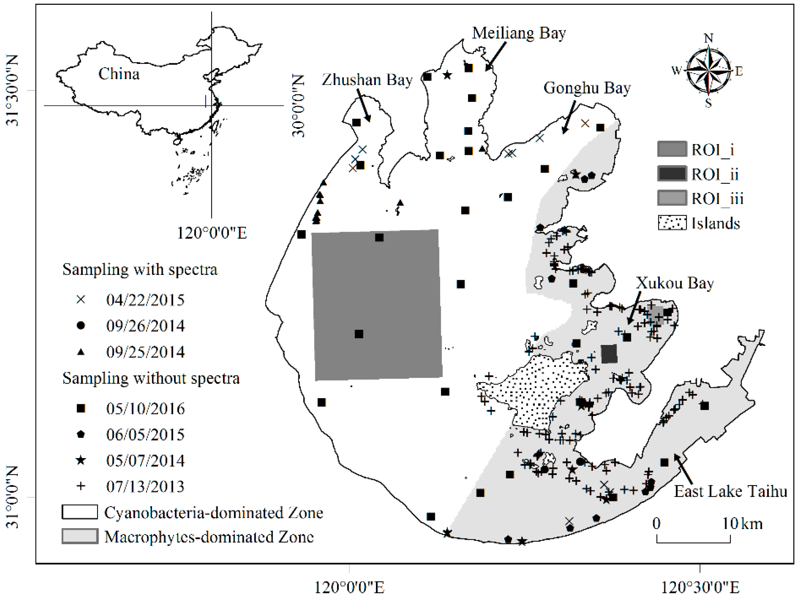
2.1. Lake Taihu
2.2. Field Data
2.3. Satellite Image Data Processing
3. Methods
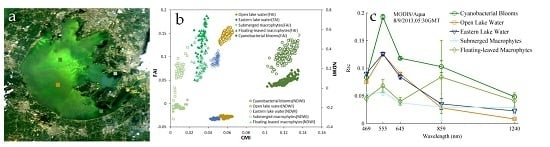
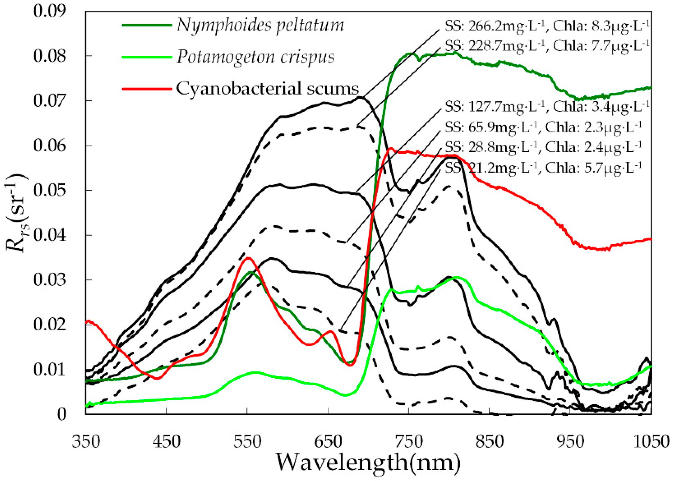
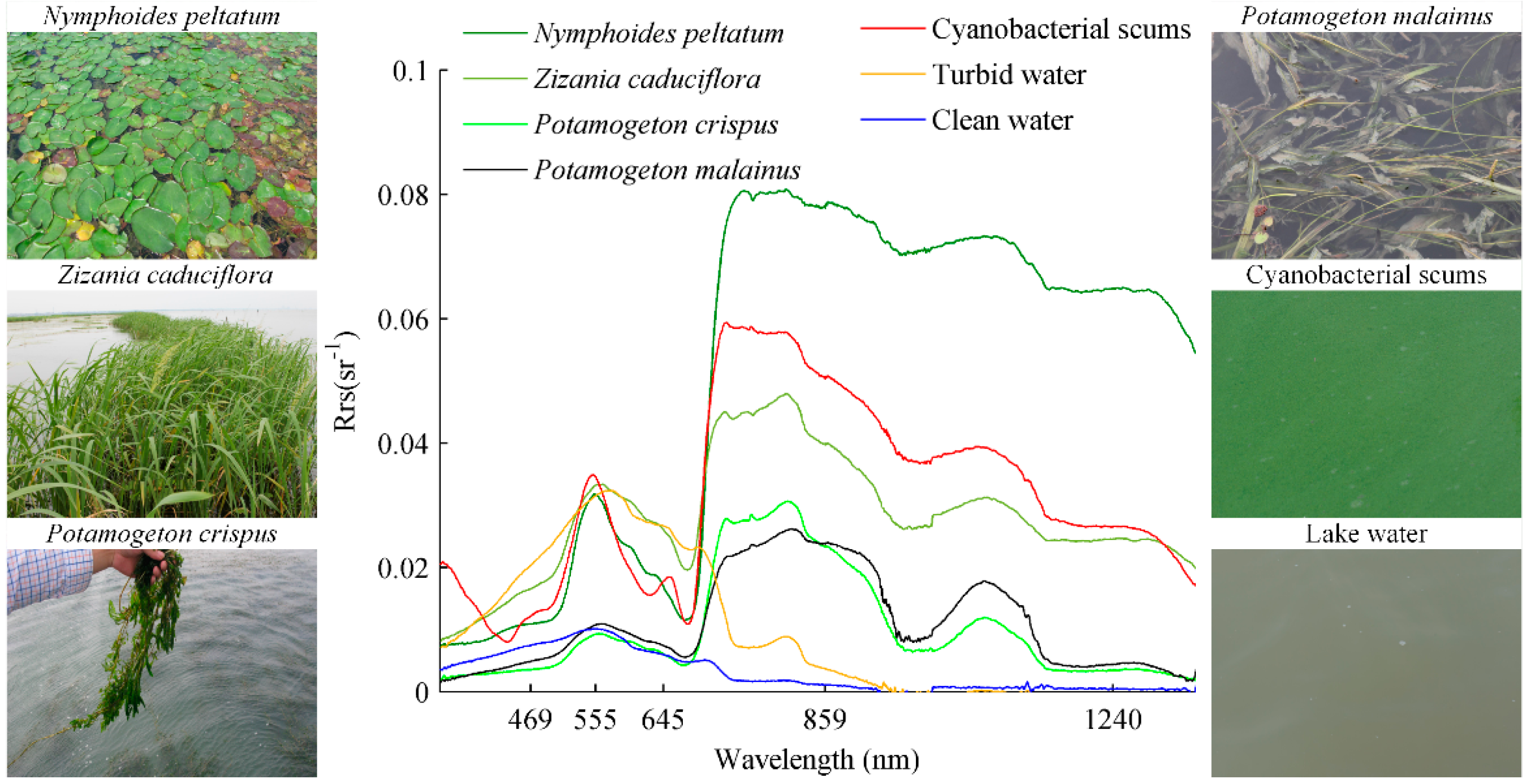
3.1. Spectral Features of Lake Water, Cyanobacterial Scums, and Aquatic Macrophytes
3.2. A New Classification Method for MODIS
3.2.1. CMI, FAI, and TWI
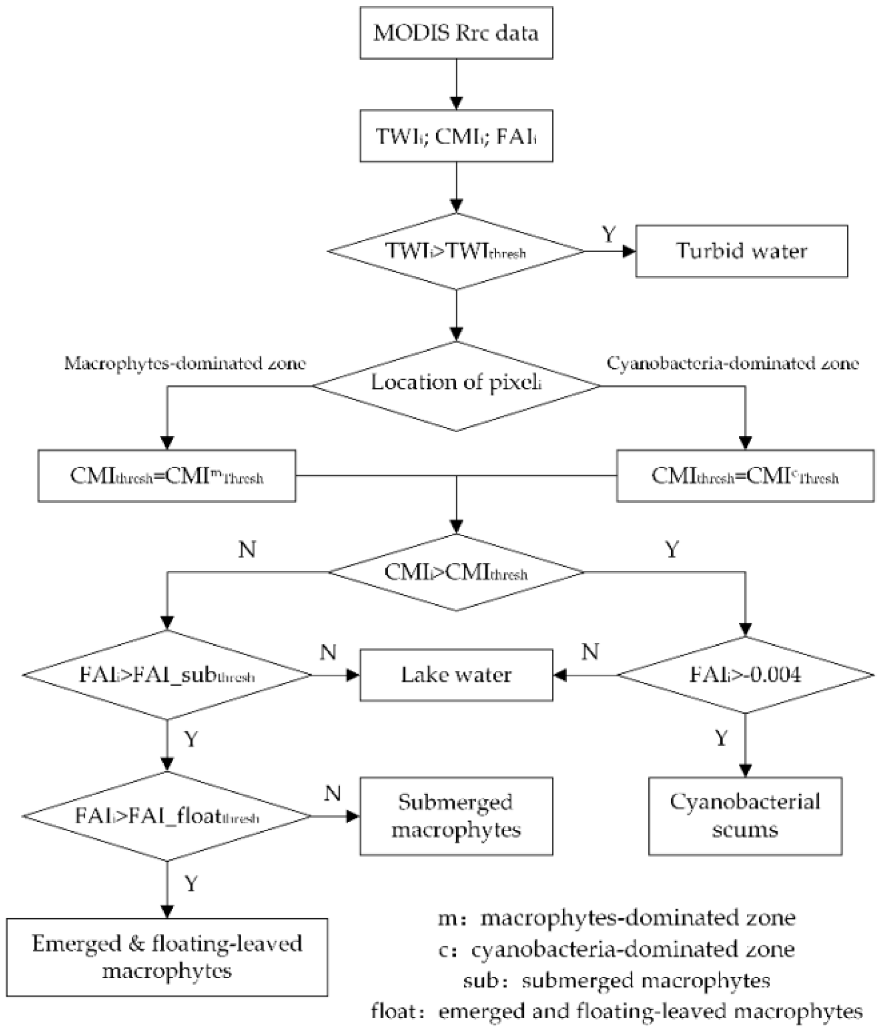
3.2.2. Classification Tree
3.2.3. Accuracy Assessment and Validation
3.3. Classification Method for HJ-CDD Data
3.4. Analysis Methods
3.4.1. Atmospheric Effects
3.4.2. Mixed Pixels Effects
4. Results
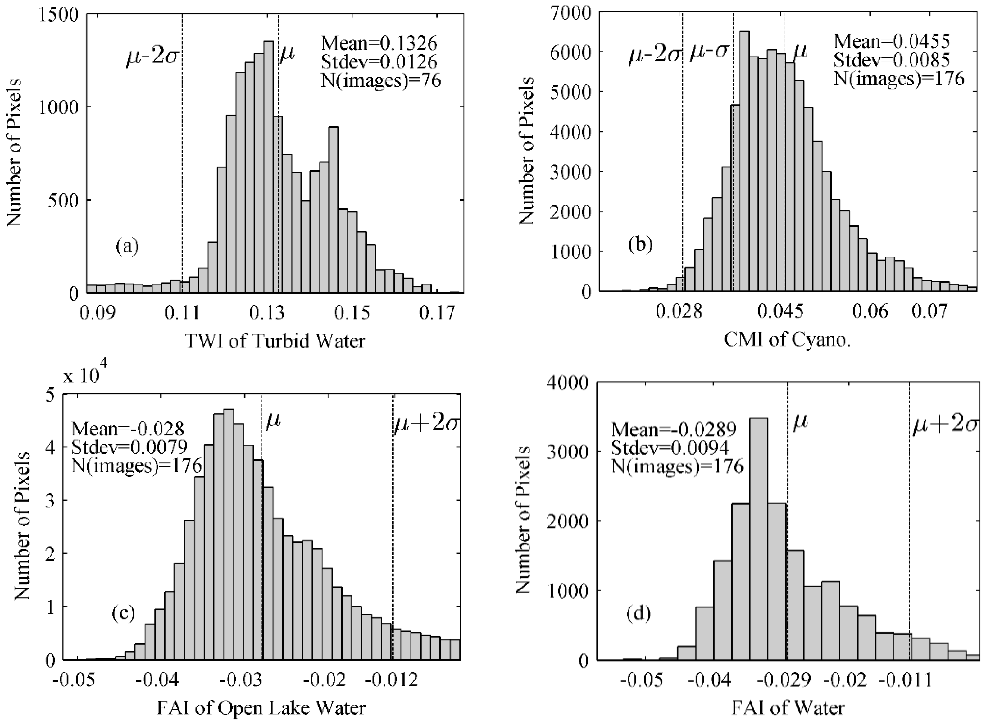
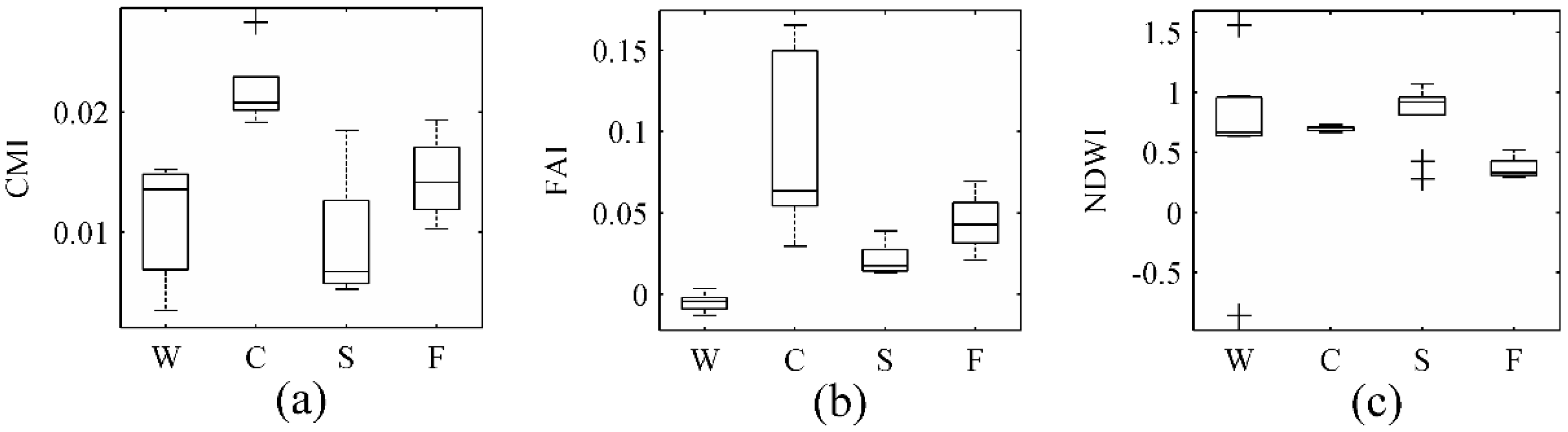
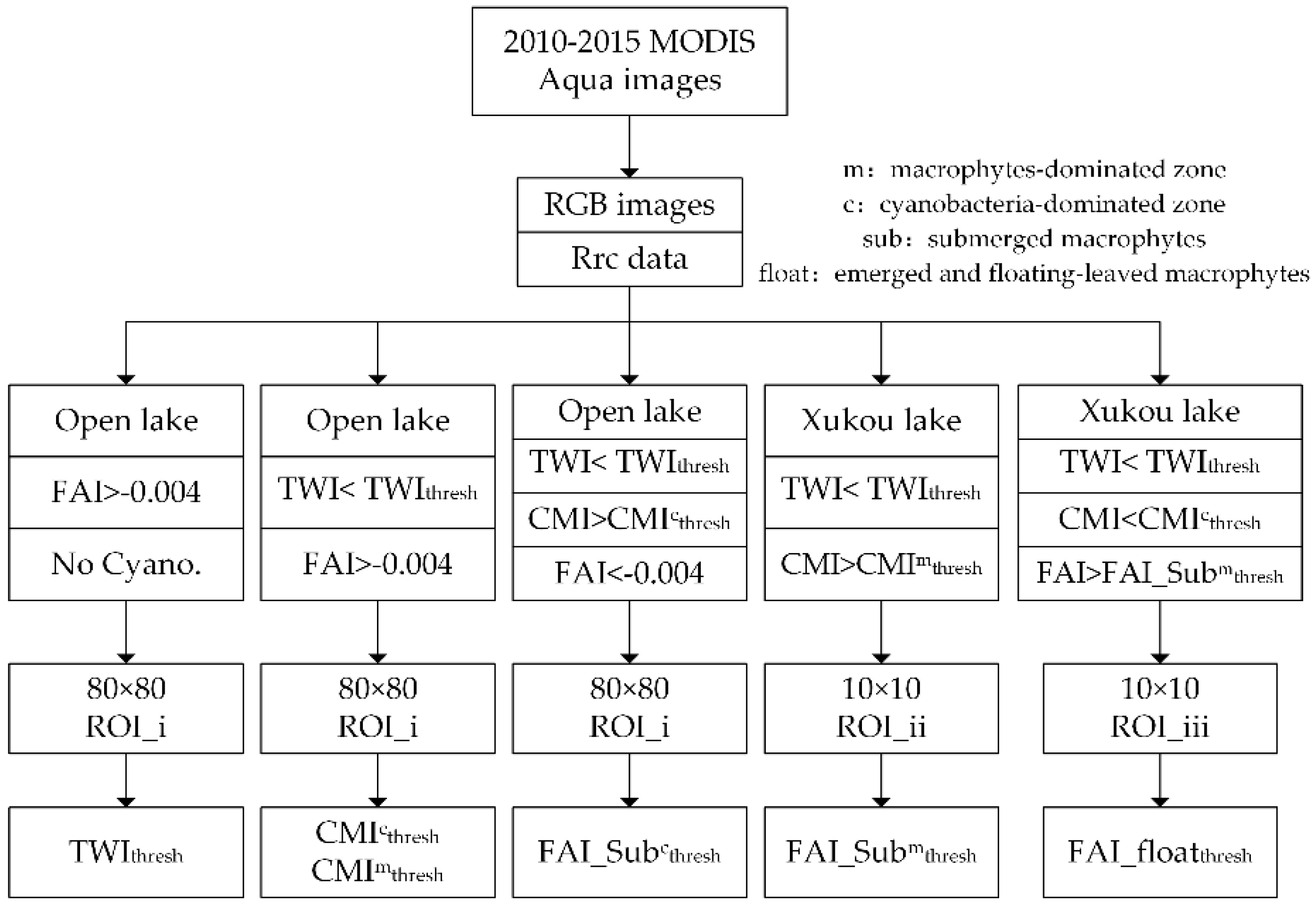
4.1. Thresholds
4.1.1. TWI Threshold Determination for Turbid Waters
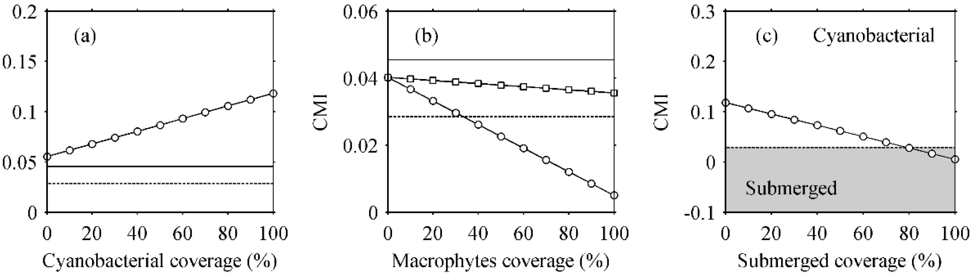
4.1.2. CMI Threshold Determination for Distinguishing Aquatic Macrophytes and Cyanobacterial Scums
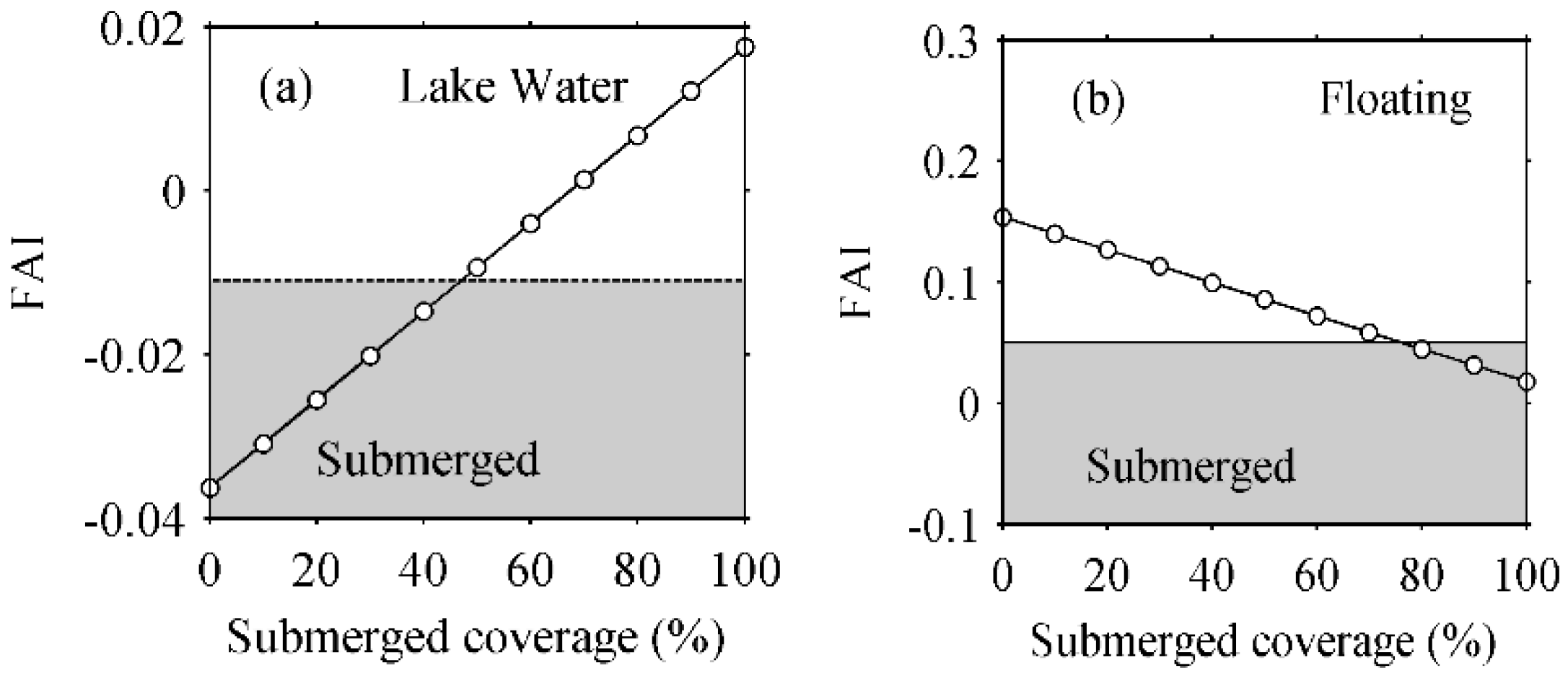
4.1.3. FAI Threshold Determination for Detection Different Types of Aquatic Macrophytes
4.2. Validation by in Situ RRS Measurements
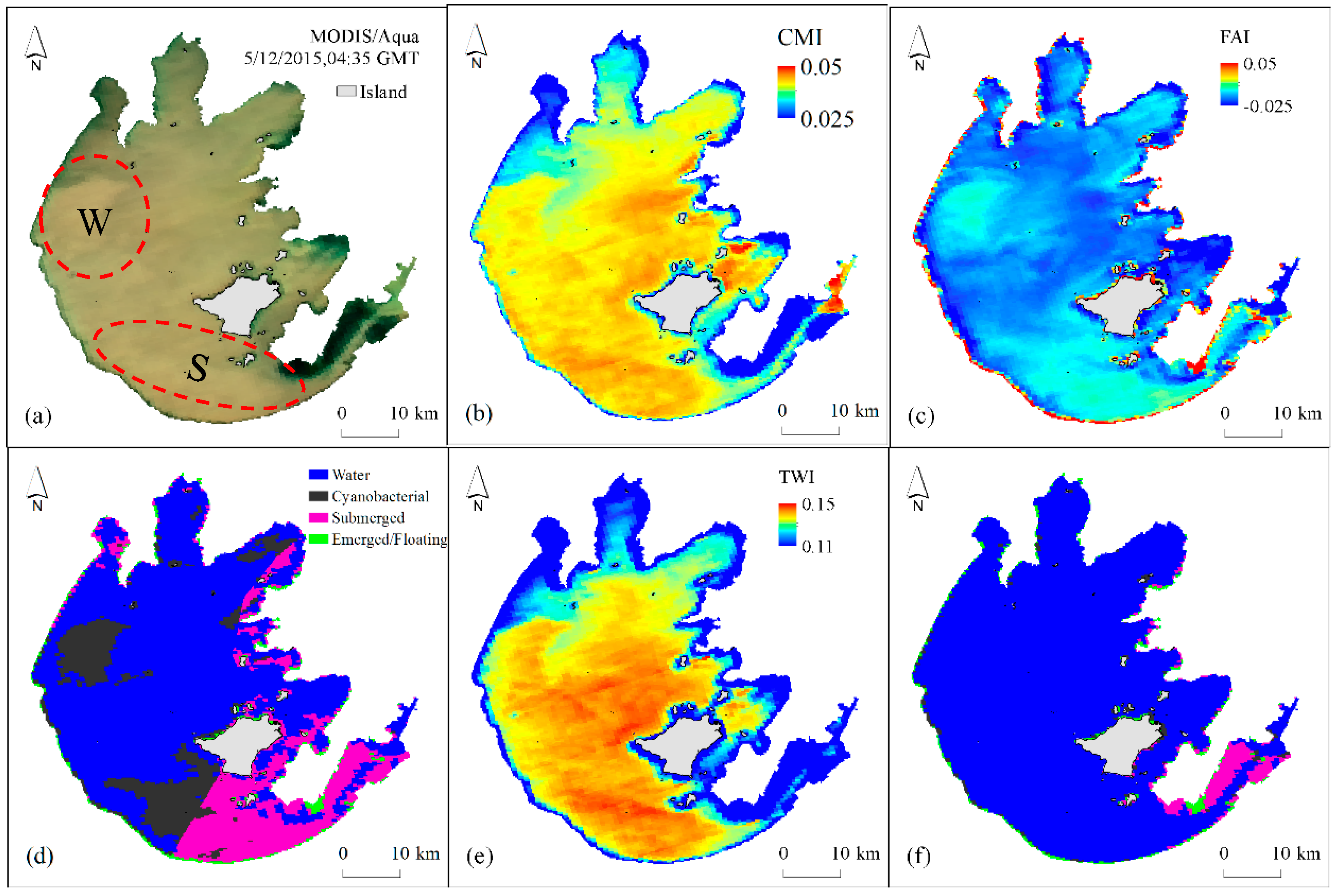
4.3. Validation by Field Investigation
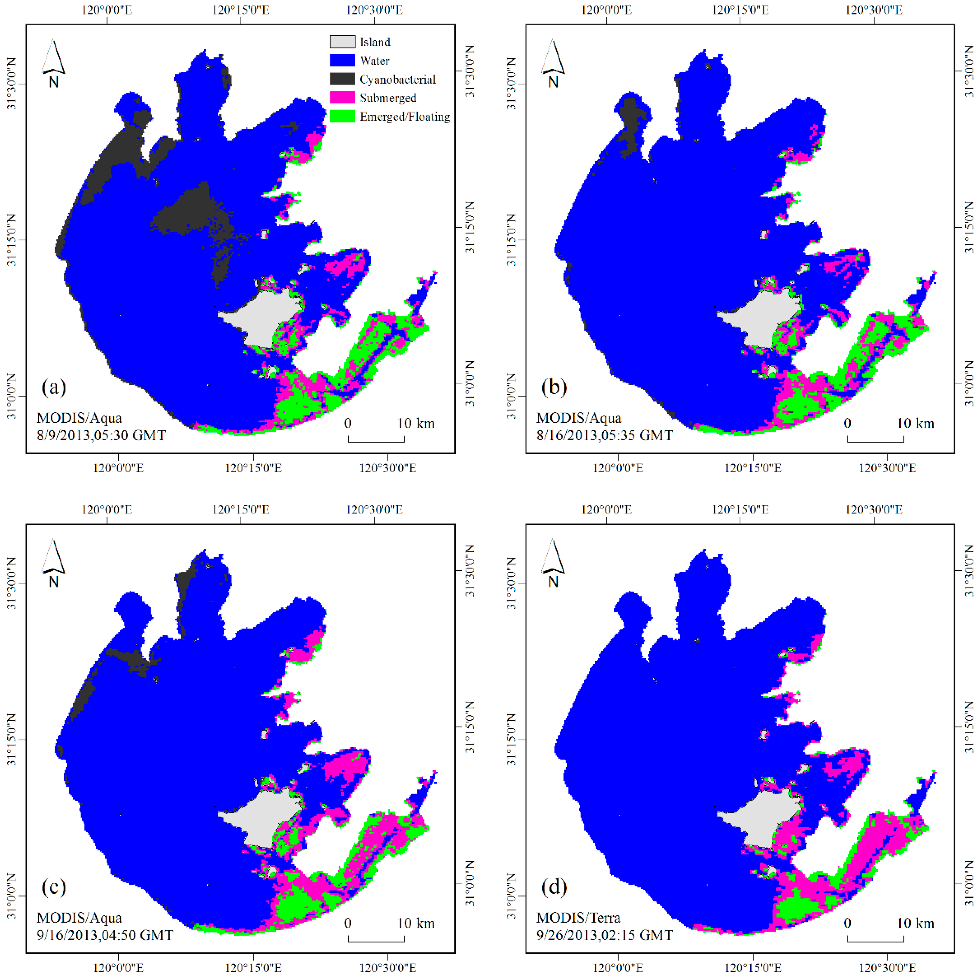
4.4. Validation by HJ-CCD Data
5. Discussion
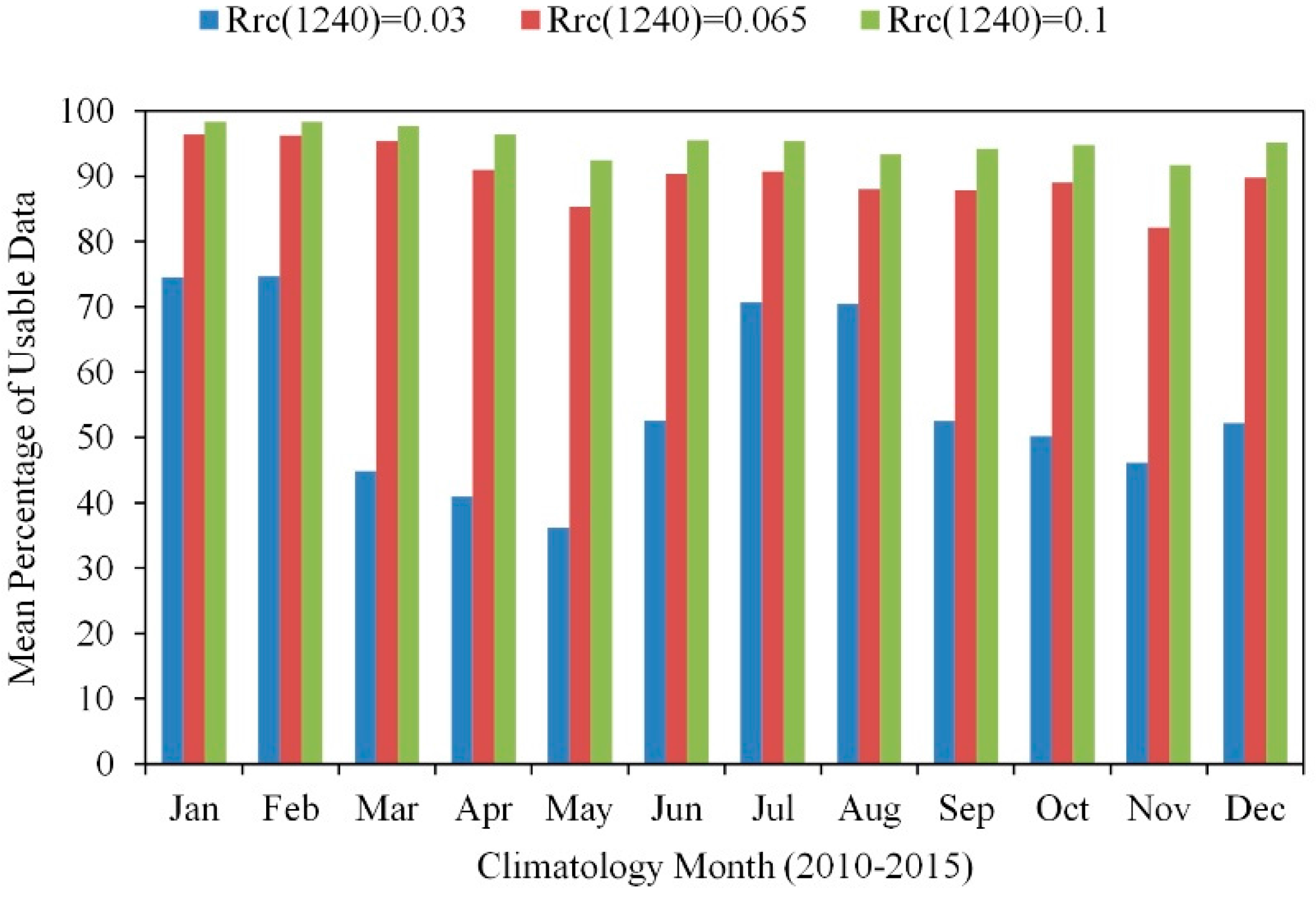
5.1. Data Quality versus Data Quantity
5.2. Use in Highly Turbid Waters
5.3. Impact of Black Waters
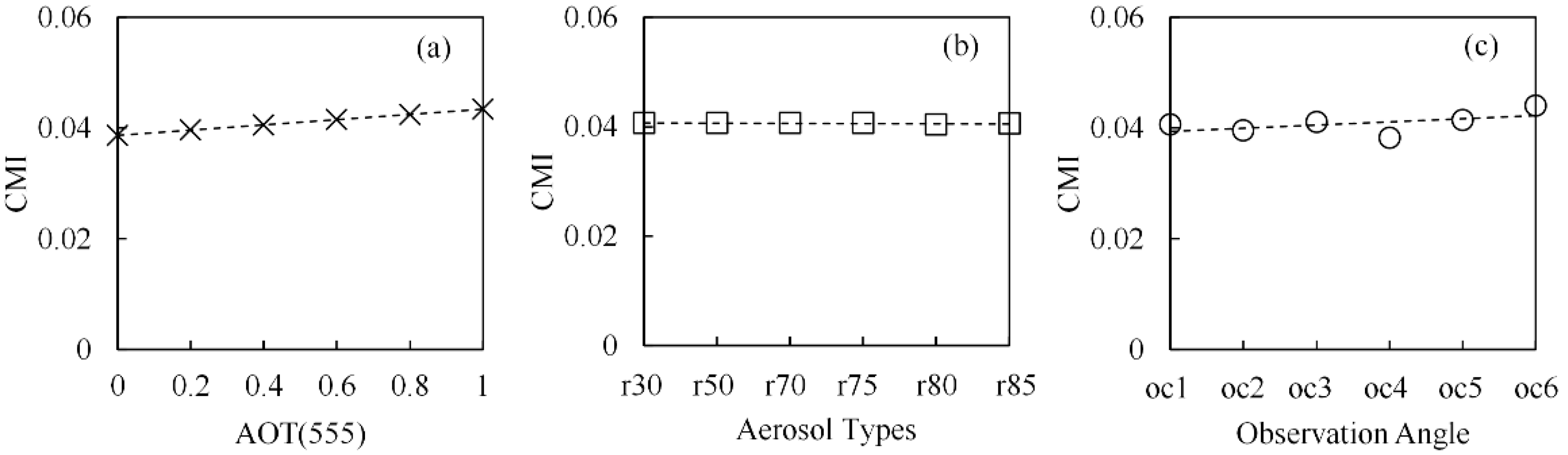
5.4. Atmospheric Effects
5.5. Mixed Pixels Effects
6. Conclusions
Acknowledgments
Author Contributions
Conflicts of Interest
References
- Huisman, J.; Matthijs, H.C.P.; Visser, P.M.E. Harmful Cyanobacteria; Springer: Dordrecht, The Netherlands, 2005. [Google Scholar]
- Granéli, E.; Turner, J.T.E. Ecology of Harmful Algae; Springer: Berlin/Heidelberg, Germany, 2006. [Google Scholar]
- Guo, L. Doing battle with the green monster of Taihu Lake. Science 2007, 317. [Google Scholar] [CrossRef] [PubMed]
- Duarte, C.M.; Middelburg, J.J.; Caraco, N. Major role of marine vegetation on the oceanic carbon cycle. Biogeosciences 2006, 2, 1–8. [Google Scholar] [CrossRef]
- Orth, R.J.; Carruthers, T.J.B.; Dennison, W.C.; Duarte, C.M.; Fourqurean, J.W.; Heck, K.L.; Hughes, A.R.; Kendrick, G.A.; Kenworthy, W.J.; Olyarnik, S.; et al. A global crisis for seagrass ecosystems. BioScience 2006, 56, 987–996. [Google Scholar] [CrossRef]
- Carr, J.; D’Odorico, P.; McGlathery, K.; Wiberg, P. Stability and bistability of seagrass ecosystems in shallow coastal lagoons: Role of feedbacks with sediment resuspension and light attenuation. J. Geophys. Res. 2010, 115. [Google Scholar] [CrossRef]
- Kolada, A. The use of aquatic vegetation in lake assessment: Testing the sensitivity of macrophyte metrics to anthropogenic pressures and water quality. Hydrobiologia 2010, 656, 133–147. [Google Scholar] [CrossRef]
- Scheffer, M.; van Nes, E.H. Shallow lakes theory revisited: Various alternative regimes driven by climate, nutrients, depth and lake size. Hydrobiologia 2007, 584, 455–466. [Google Scholar] [CrossRef]
- Xue, K.; Zhang, Y.; Duan, H.; Ma, R.; Loiselle, S.; Zhang, M. A remote sensing approach to estimate vertical profile classes of phytoplankton in a eutrophic lake. Remote Sens. 2015, 7, 14403–14427. [Google Scholar] [CrossRef]
- Walsby, A.E. Gas vesicles. Microbiol. Rev. 1994, 58, 94–144. [Google Scholar] [CrossRef] [PubMed]
- Matthews, M.W. A current review of empirical procedures of remote sensing in inland and near-coastal transitional waters. Int. J. Remote Sens. 2011, 32, 6855–6899. [Google Scholar] [CrossRef]
- Odermatt, D.; Gitelson, A.; Brando, V.E.; Schaepman, M. Review of constituent retrieval in optically deep and complex waters from satellite imagery. Remote Sens. Environ. 2012, 118, 116–126. [Google Scholar] [CrossRef] [Green Version]
- Patissier, D.B.; Gower, J.F.R.; Dekker, A.G.; Phinn, S.R.; Brando, V.E. A review of ocean color remote sensing methods and statistical techniques for the detection, mapping and analysis of phytoplankton blooms in coastal and open oceans. Prog. Oceanogr. 2014, 123, 123–144. [Google Scholar] [CrossRef] [Green Version]
- Peñuelas, J.; Gamon, J.A.; Griffin, K.L.; Field, C.B. Assessing community type, plant biomass, pigment composition, and photosynthetic efficiency of aquatic vegetation from spectral reflectance. Remote Sens. Environ. 1993, 46, 110–118. [Google Scholar] [CrossRef]
- Gitelson, A.A.; Kaufman, Y.J.; Stark, R.; Rundquist, D.C. Novel algorithms for remote estimation of vegetation fraction. Remote Sens. Environ. 2002, 80, 76–87. [Google Scholar] [CrossRef]
- Silva, T.S.; Costa, M.P.; Melack, J.M.; Novo, E.M. Remote sensing of aquatic vegetation: Theory and applications. Environ. Monit. Assess. 2008, 140, 131–145. [Google Scholar] [CrossRef] [PubMed]
- Olmanson, L.G.; Bauer, M.E.; Brezonik, P.L. A 20-year Landsat water clarity census of Minnesota’s 10,000 lakes. Remote Sens. Environ. 2008, 112, 4086–4097. [Google Scholar] [CrossRef]
- Bresciani, M.; Adamo, M.; De Carolis, G.; Matta, E.; Pasquariello, G.; Vaičiūtė, D.; Giardino, C. Monitoring blooms and surface accumulation of cyanobacteria in the curonian lagoon by combining MERIS and ASAR data. Remote Sens. Environ. 2014, 146, 124–135. [Google Scholar] [CrossRef]
- Duan, H.; Ma, R.; Xu, X.; Kong, F.; Zhang, S.; Kong, W.; Hao, J.; Shang, L. Two-decade reconstruction of algal blooms in China’s lake Taihu. Environ. Sci. Technol. 2009, 43, 3522–3528. [Google Scholar] [CrossRef] [PubMed]
- Kahru, M.; Savchuk, O.P.; Elmgren, R. Satellite measurements of cyanobacterial bloom frequency in the Baltic Sea: Interannual and spatial variability. Mar. Ecol. Prog. Ser. 2007, 343, 15–23. [Google Scholar] [CrossRef]
- Kahru, M.; Elmgren, R. Multidecadal time series of satellite-detected accumulations of cyanobacteria in the Baltic Sea. Biogeosciences 2014, 11, 3619–3633. [Google Scholar] [CrossRef] [Green Version]
- Groom, S.B.; Holligan, P.M. Remote sensing of coccolithophore blooms. Adv. Space Res. 1987, 7, 73–78. [Google Scholar] [CrossRef]
- Duan, H.; Zhang, S.; Zhang, Y. Cyanobacteria bloom monitoring with remote sensing in Lake Taihu. J. Lake Sci. 2008, 20, 145–152. (In Chinese) [Google Scholar]
- Ma, R.; Kong, F.; Duan, H.; Zhang, S.; Kong, W.; Hao, J. Spatiotemporal distribution of cyanobacterial scums based on satellite imageries in Lake Taihu, China. J. Lake Sci. 2008, 20, 687–694. (In Chinese) [Google Scholar]
- Son, Y.B.; Min, J.E.; Ryu, J.H. Detecting massive green algae (Ulva prolifera) blooms in the Yellow Sea and East China Sea using geostationary ocean color imager (GOCI) data. Ocean Sci. J. 2012, 47, 359–375. [Google Scholar] [CrossRef]
- Stumpf, R.P.; Tomlinson, M.C. Remote sensing of harmful algal blooms. Remote Sens. Coast. Aquat. Environ. 2005, 7, 277–296. [Google Scholar]
- Holligan, P.M.; Viollier, M.; Harbour, D.S.; Camus, P.; Philippe, M.C. Satellite and ship studies of coccolithophore production along a continental shelf edge. Nature 1983, 304, 339–342. [Google Scholar] [CrossRef]
- Gitelson, A.; Karnieli, A.; Goldman, N.; Yacobi, Y.Z.; Mayo, M. Chlorophyll estimation in the southeastern Mediterranean using CZCS images: Adaption of an algorithm and its validation. J. Mar. Syst. 1996, 9, 283–290. [Google Scholar] [CrossRef]
- Kopelevich, O.V.; Sheberstov, S.V.; Yunev, O.; Basturk, O.; Finenko, Z.Z.; Nikonov, S.; Vedernikov, V.I. Surface chlorophyll in the Black Sea over 1978–1986 derived from satellite and in situ data. J. Mar. Syst. 2002, 36, 145–160. [Google Scholar] [CrossRef]
- Gower, J.F.R. Red tide monitoring using AVHRR HRPT imagery from a local receiver. Remote Sens. Environ. 1994, 48, 309–318. [Google Scholar] [CrossRef]
- Kahru, M.; Mitchell, B.G.; Diaz, A.; Miura, M. MODIS detects a devastating algal bloom in Paracas Bay, Peru. EOS Trans. Am. Geophys. Union 2004, 85, 465–472. [Google Scholar] [CrossRef]
- Rouse, J.W.; Haas, R.H.; Schell, J.A.; Deering, D.W. Monitoring vegetation systems in the Great Plains with ERTS-1. In 3rd Earth Resources Technology Satellite Symposium; NASA: Washington, DC, USA, 1973; pp. 309–317. [Google Scholar]
- Hu, C.; He, M. Origin and offshore extent of floating algae in Olympic sailing area. EOS Trans. Am. Geophys. Union 2008, 89, 302–303. [Google Scholar] [CrossRef]
- Garcia, R.A.; Fearns, P.; Keesing, J.K.; Liu, D. Quantification of floating macroalgae blooms using the scaled algae index. J. Geophys. Res. Oceans 2013, 118, 26–42. [Google Scholar] [CrossRef]
- Prangsma, G.J.; Roozekrans, J.N. Using NOAA AVHRR imagery in assessing water quality parameters. Int. J. Remote Sens. 1989, 10, 811–818. [Google Scholar] [CrossRef]
- Huete, A.; Justice, C.; Leeuwen, W.V. MODIS Vegetation Index (MOD13) Algorithm Theoretical Basis Document (Ver 3.0); NASA: Washington, DC, USA, 1999.
- Wynne, T.T.; Stumpf, R.P.; Tomlinson, M.C.; Dybleb, J. Characterizing a cyanobacterial bloom in western Lake Erie using satellite imagery and meteorological data. Limnol. Oceanogr. 2010, 55, 2025–2036. [Google Scholar] [CrossRef] [Green Version]
- Gower, J.F.R.; Doerffer, R.; Borstad, G.A. Interpretation of the 685nm peak in water-leaving radiance spectra in terms of fluorescence, absorption and scattering, and its observation by MERIS. Int. J. Remote Sens. 1999, 20, 1771–1786. [Google Scholar] [CrossRef]
- Gower, J.; King, S.; Borstad, G.; Brown, L. Detection of intense plankton blooms using the 709 nm band of the MERIS imaging spectrometer. Int. J. Remote Sens. 2005, 26, 2005–2012. [Google Scholar] [CrossRef]
- Wynne, T.T.; Stumpf, R.P.; Tomlinson, M.C.; Warner, R.A.; Tester, P.A.; Dyble, J.; Fahnenstiel, G.L. Relating spectral shape to cyanobacterial scums in the Laurentian Great Lakes. Int. J. Remote Sens. 2008, 29, 3665–3672. [Google Scholar] [CrossRef]
- Wynne, T.T.; Stumpf, R.P.; Briggs, T.O. Comparing MODIS and MERIS spectral shapes for cyanobacterial bloom detection. Int. J. Remote Sens. 2013, 34, 6668–6678. [Google Scholar] [CrossRef]
- Wynne, T.T.; Stumpf, R.P.; Tomlinson, M.C.; Fahnenstiel, G.L.; Dyble, J.; Schwab, D.J.; Joshi, S.J. Evolution of a cyanobacterial bloom forecast system in western lake Erie: Development and initial evaluation. J. Great Lakes Res. 2013, 39, 90–99. [Google Scholar] [CrossRef]
- Stumpf, R.P.; Wynne, T.T.; Baker, D.B.; Fahnenstiel, G.L. Interannual variability of cyanobacterial scums in lake Erie. PLoS ONE 2012, 7. [Google Scholar] [CrossRef] [PubMed]
- Matthews, M.W.; Bernard, S.; Robertson, L. An algorithm for detecting trophic status (chlorophyll-a), cyanobacterial-dominance, surface scums and floating vegetation in inland and coastal waters. Remote Sens. Environ. 2012, 124, 637–652. [Google Scholar] [CrossRef]
- Matthews, M.W.; Odermatt, D. Improved algorithm for routine monitoring of cyanobacteria and eutrophication in inland and near-coastal waters. Remote Sens. Environ. 2015, 156, 374–382. [Google Scholar] [CrossRef]
- Hu, C. A novel ocean color index to detect floating algae in the global oceans. Remote Sens. Environ. 2009, 113, 2118–2129. [Google Scholar] [CrossRef]
- Hu, C.H.; Lee, Z.L.; Ma, R.M.; Yu, K.; Li, D. Moderate resolution imaging spectroradiometer (MODIS) observations of cyanobacteria blooms in Taihu Lake, China. J. Geophys. Res. 2010, 115. [Google Scholar] [CrossRef]
- Hu, C.; Cannizzaro, J.; Carder, K.L.; Karger, F.E.M.; Hardya, R. Remote detection of Trichodesmium blooms in optically complex coastal waters: Examples with MODIS full-spectral data. Remote Sens. Environ. 2010, 114, 2048–2058. [Google Scholar] [CrossRef]
- Huang, C.; Li, Y.; Yang, H.; Sun, D.; Yu, Z.; Zhang, Z.; Chen, X.; Xu, L. Detection of algal bloom and factors influencing its formation in Taihu lake from 2000 to 2011 by MODIS. Environ. Earth Sci. 2014, 71, 3705–3714. [Google Scholar] [CrossRef]
- Zhang, Y.; Ma, R.; Zhang, M.; Duan, H.; Loiselle, S.; Xu, J. Fourteen-year record (2000–2013) of the spatial and temporal dynamics of floating algae blooms in lake Chaohu, observed from time series of MODIS images. Remote Sens. 2015, 7, 10523–10542. [Google Scholar] [CrossRef]
- Alem, A.E.; Chokmani, K.; Laurion, I.; Adlouni, S.E. An adaptive model to monitor chlorophyll-a in inland waters in southern Quebec using downscaled MODIS imagery. Remote Sens. 2014, 6, 6446–6471. [Google Scholar] [CrossRef]
- Work, E.A.; Gilmer, D.S. Utilization of satellite data for inventorying prairie ponds and potholes. Photogramm. Eng. Remote Sens. 1976, 42, 685–694. [Google Scholar]
- Kempka, R.G.; Kollasch, R.P.; Koeln, G.T. Ducks unlimited: Using GIS to preserve the pacific flyway’s wetland resource. GIS World 1992, 5, 46–52. [Google Scholar]
- Jakubauskas, M.; Kindscher, K.; Debinski, D. Multitemporal characterization and mapping of montane sagebrush communities using Indian IRS LISS-II imagery. Geocarto Int. 1998, 13, 65–74. [Google Scholar] [CrossRef]
- Macleod, R.D.; Congalton, R.G. A quantitative comparison of change-detection algorithms for monitoring eelgrass from remotely sensed data. Photogramm. Eng. Remote Sens. 1998, 64, 207–216. [Google Scholar]
- Gullström, M.; Lundén, B.; Bodin, M.; Kangwe, J.; Öhman, M.C.; Mtolera, M.S.P.; Björk, M. Assessment of changes in the seagrass-dominated submerged vegetation of tropical Chwaka bay (Zanzibar) using satellite remote sensing. Estuar. Coast. Shelf Sci. 2006, 67, 399–408. [Google Scholar] [CrossRef]
- Dogan, O.K.; Akyurek, Z.; Beklioglu, M. Identification and mapping of submerged plants in a shallow lake using Quickbird satellite data. J. Environ. Manag. 2009, 90, 2138–2143. [Google Scholar] [CrossRef] [PubMed]
- Hewitt, M.J. Synoptic inventory of riparian ecosystems: The utility of Landsat thematic mapper data. For. Ecol. Manag. 1990, 33–34, 605–620. [Google Scholar] [CrossRef]
- MacAlister, C.; Mahaxay, M. Mapping wetlands in the lower Mekong Basin for wetland resource and conservation management using Landsat ETM images and field survey data. J. Environ. Manag. 2009, 90, 2130–2137. [Google Scholar] [CrossRef] [PubMed]
- De Colstoun, E.B. National park vegetation mapping using multitemporal Landsat 7 data and a decision tree classifier. Remote Sens. Environ. 2003, 85, 316–327. [Google Scholar] [CrossRef]
- Baker, C.; Lawrence, R.; Montagne, C.; Patten, D. Mapping wetlands and riparian areas using Landsat ETM+ imagery and decision-tree-based models. Wetlands 2006, 26, 465–474. [Google Scholar] [CrossRef]
- Wright, C.; Gallant, A. Improved wetland remote sensing in Yellowstone national park using classification trees to combine tm imagery and ancillary environmental data. Remote Sens. Environ. 2007, 107, 582–605. [Google Scholar] [CrossRef]
- Davranche, A.; Lefebvre, G.; Poulin, B. Wetland monitoring using classification trees and SPOT-5 seasonal time series. Remote Sens. Environ. 2010, 114, 552–562. [Google Scholar] [CrossRef] [Green Version]
- Zhao, D.; Jiang, H.; Yang, T.; Cai, Y.; Xu, D.; An, S. Remote sensing of aquatic vegetation distribution in Taihu lake using an improved classification tree with modified thresholds. J. Environ. Manag. 2012, 95, 98–107. [Google Scholar] [CrossRef] [PubMed]
- Zhao, D.; Lv, M.; Jiang, H.; Cai, Y.; Xu, D.; An, S. Spatio-temporal variability of aquatic vegetation in Taihu lake over the past 30 years. PLoS ONE 2013, 8. [Google Scholar] [CrossRef] [PubMed]
- Luo, J.; Ma, R.; Duan, H.; Hu, W.; Zhu, J.; Huang, W.; Lin, C. A new method for modifying thresholds in the classification of tree models for mapping aquatic vegetation in Taihu Lake with satellite images. Remote Sens. 2014, 6, 7442–7462. [Google Scholar] [CrossRef]
- Oyama, Y.; Matsushita, B.; Fukushima, T. Distinguishing surface cyanobacterial scums and aquatic macrophytes using Landsat/TM and ETM+ shortwave infrared bands. Remote Sens. Environ. 2015, 157, 35–47. [Google Scholar] [CrossRef]
- Liu, X.; Zhang, Y.; Shi, K.; Zhou, Y.; Tang, X.; Zhu, G.; Qin, B. Mapping aquatic vegetation in a large, shallow eutrophic lake: A frequency-based approach using multiple years of MODIS data. Remote Sens. 2015, 7, 10295–10320. [Google Scholar] [CrossRef]
- Zhang, Y.; Liu, X.; Qin, B.; Shi, K.; Deng, J.; Zhou, Y. Aquatic vegetation in response to increased eutrophication and degraded light climate in eastern lake Taihu: Implications for lake ecological restoration. Sci. Rep. 2016, 6. [Google Scholar] [CrossRef] [PubMed]
- Gao, B.C. NDWI—A normalized difference water index for remote sensing of vegetation liquid water from space. Remote Sens. Environ. 1996, 58, 257–266. [Google Scholar] [CrossRef]
- Rogers, A.; Kearney, M. Reducing signature variability in unmixing coastal marsh thematic mapper scenes using spectral indices. Int. J. Remote Sens. 2004, 25, 2317–2335. [Google Scholar] [CrossRef]
- Qi, L.; Hu, C.; Duan, H.; Cannizzaro, J.; Ma, R. A novel meris algorithm to derive cyanobacterial phycocyanin pigment concentrations in a eutrophic lake: Theoretical basis and practical considerations. Remote Sens. Environ. 2014, 154, 298–317. [Google Scholar] [CrossRef]
- Qi, L.; Hu, C.; Duan, H.; Barnes, B.; Ma, R. An EOF-based algorithm to estimate chlorophyll a concentrations in Taihu Lake from MODIS land-band measurements: Implications for near real-time applications and forecasting models. Remote Sens. 2014, 6, 10694–10715. [Google Scholar] [CrossRef]
- Palmer, S.C.J.; Hunter, P.D.; Lankester, T.; Hubbard, S.; Spyrakos, E.; Tyler, A.N.; Présing, M.; Horváth, H.; Lamb, A.; Balzter, H.; et al. Validation of ENVISAT Meris algorithms for chlorophyll retrieval in a large, turbid and optically-complex shallow lake. Remote Sens. Environ. 2015, 157, 158–169. [Google Scholar] [CrossRef] [Green Version]
- Hu, C.; Chen, Z.; Clayton, T.D.; Swarzenski, P.; Brock, J.C.; Muller-Karger, F.E. Assessment of estuarine water-quality indicators using MODIS medium-resolution bands: Initial results from Tampa bay, FL. Remote Sens. Environ. 2004, 93, 423–441. [Google Scholar] [CrossRef]
- Le, C.; Hu, C.; English, D.; Cannizzaro, J.; Chen, Z.; Feng, L.; Boler, R.; Kovach, C. Towards a long-term chlorophyll-a data record in a turbid estuary using MODIS observations. Prog. Oceanogr. 2013, 109, 90–103. [Google Scholar] [CrossRef]
- Qin, B.Q.; Hu, W.P.; Chen, W.M. Process and Mechanism of Environmental Changes of the Taihu Lake; Science Press: Beijing, China, 2004. [Google Scholar]
- Qin, B.; Xu, P.; Wu, Q.; Luo, L.; Zhang, Y. Environmental issues of lake Taihu, China. Hydrobiologia 2007, 581, 3–14. [Google Scholar] [CrossRef]
- Ma, R.; Duan, H.; Gu, X.; Zhang, S. Detecting aquatic vegetation changes in Taihu lake, China using multi-temporal satellite imagery. Sensors 2008, 8, 3988–4005. [Google Scholar] [CrossRef] [PubMed]
- Kalff, J. Limnology: Inland Water Ecosystems; Prentice Hall: Upper Saddle River, NJ, USA, 2002. [Google Scholar]
- Lei, Z. Study on Aquatic Macrophyte Vegetations and Their Environment Effects in Taihu Lake. Ph.D. Thesis, Jinan University, Jinan, China, 2006. [Google Scholar]
- Mueller, J.L.; Fargion, G.S.; McClain, C.R. Ocean Optics Protocols for Satellite Ocean Color Sensor Validation, Revision 4. Volume VI: Special Topics in Ocean Optics Protocols and Appendices; NASA Goddard Space Flight Center: Greenbelt, MD, USA, 2003.
- Mobley, C.D. Estimation of the remote-sensing reflectance from above-surface measurements. Appl. Opt. 1999, 38, 7442–7455. [Google Scholar] [CrossRef] [PubMed]
- Ahn, Y.H.; Shanmugam, P. Detecting the red tide algal blooms from satellite ocean color observations in optically complex Northeast-Asia coastal waters. Remote Sens. Environ. 2006, 103, 419–437. [Google Scholar] [CrossRef]
- Dev, P.J.; Shanmugam, P. A new theory and its application to remove the effect of surface-reflected light in above-surface radiance data from clear and turbid waters. J. Quant. Spectrosc. Radiat. Transf. 2014, 142, 75–92. [Google Scholar] [CrossRef]
- Sun, D.; Hu, C.; Qiu, Z.; Shi, K. Estimating phycocyanin pigment concentration in productive inland waters using Landsat measurements: A case study in lake Dianchi. Opt. Exp. 2015, 23, 3055–3074. [Google Scholar] [CrossRef] [PubMed]
- NASA’s OceanColor Web. Available online: http://oceancolor.gsfc.nasa.gov (accessed on 16 December 2016).
- Gordon, H.R.; Clark, D.K. Clear water radiances for atmospheric correction of coastal zone color scanner imagery. Appl. Opt. 1981, 20, 4175–4180. [Google Scholar] [CrossRef] [PubMed]
- Ruddick, K.G.; Ovidio, F.; Rijkeboer, M. Atmospheric correction of SeaWIFS imagery for turbid coastal and inland waters. Appl. Opt. 2000, 39, 897–912. [Google Scholar] [CrossRef] [PubMed]
- Wang, M.; Shi, W. The NIR-SWIR combined atmospheric correction approach for MODIS ocean color data processing. Opt. Exp. 2007, 15, 15722–15733. [Google Scholar] [CrossRef]
- Bailey, S.W.; Franz, B.A.; Werdell, P.J. Estimation of near-infrared water-leaving reflectance for satellite ocean color data processing. Opt. Express 2010, 18, 7521–7527. [Google Scholar] [CrossRef] [PubMed]
- Reinart, A.; Herlevi, A.; Arst, H.; Sipelgas, L. Preliminary optical classification of lakes and coastal waters in Estonia and South Finland. J. Sea Res. 2003, 49, 357–366. [Google Scholar] [CrossRef]
- Gitelson, A.A.; Dall’Olmo, G.; Moses, W.M.; Rundquist, D.C.; Barrow, T.; Fisher, T.R.; Gurlin, D.; Holz, J. A simple semi-analytical model for remote estimation of chlorophyll-a in turbidwaters: Validation. Remote Sens. Environ. 2008, 112, 3582–3593. [Google Scholar] [CrossRef]
- Bricaud, A.; Roesler, C.; Zaneveld, J.R.V. In situ methods for measuring the inherent optical properties of ocean waters. Limnol. Oceanogr. 1995, 40, 393–410. [Google Scholar] [CrossRef]
- Dekker, A.G.; Malthus, T.J.; Goddijn, L.M. Monitoring cyanobacteria in eutrophic waters using airborne imaging spectroscopy and multispectral remote sensing systems. In Proceedings of the 6th Australasian Remote Sensing Conference, Wellington, NZ, USA, 2–6 November 1992; pp. 204–214.
- Le, C.; Li, Y.; Zha, Y.; Sun, D.; Huang, C.; Lu, H. A four-band semi-analytical model for estimating chlorophyll a in highly turbid lakes: The case of Taihu Lake, China. Remote Sens. Environ. 2009, 113, 1175–1182. [Google Scholar] [CrossRef]
- Hoffer, R.M. Biological and physical considerations in applying computer-aided analysis techniques to remote sensor data. In Remote Sensing: The Quantitative Approach; Swain, P.H., Davis, S.M., Eds.; McGraw-Hill: New York, NY, USA, 1978; pp. 227–289. [Google Scholar]
- Feng, L.; Hu, C.; Chen, X.; Cai, X.; Tian, L.; Chen, L. Human induced turbidity changes in Poyang Lake between 2000 and 2010: Observations from MODIS. J. Geophys. Res. 2012, 117. [Google Scholar] [CrossRef]
- Foody, G.M. Local characterization of thematic classification accuracy through spatially constrained confusion matrices. Int. J. Remote Sens. 2005, 26, 1217–1228. [Google Scholar] [CrossRef]
- Congalton, R.G. A review of assessing the accuracy of classifications of remotely sensed data. Remote Sens. Environ. 1991, 37, 35–46. [Google Scholar] [CrossRef]
- New Hampshire View Web. Available online: http://www.nhview.unh.edu/accuracyprograms.html (accessed on 16 December 2016).
- Wang, M.; Shi, W. Cloud masking for ocean color data processing in the coastal regions. IEEE Trans. Geosci. Remote Sens. 2006, 44, 3196–3205. [Google Scholar] [CrossRef]
- Ma, R.; Duan, H.; Liu, Q.; Loiselle, S.A. Approximate bottom contribution to remote sensing reflectance in Taihu Lake, China. J. Great Lakes Res. 2011, 37, 18–25. [Google Scholar] [CrossRef]
- Duan, H.; Ma, R.; Loiselle, S.A.; Shen, Q.; Yin, H.; Zhang, Y. Optical characterization of black water blooms in eutrophic waters. Sci. Total Environ. 2014, 482–483, 174–183. [Google Scholar] [CrossRef] [PubMed]
- Zhao, J.; Hu, C.; Lapointe, B.; Melo, N.; Johns, E.; Smith, R. Satellite-observed black water events off southwest florida: Implications for coral reef health in the Florida keys national marine sanctuary. Remote Sens. 2013, 5, 415–431. [Google Scholar] [CrossRef]
- Yang, M.; Yu, J.W.; Li, Z.L.; Guo, Z.H.; Burch, M.; Lin, T.F. Taihu lake not to blame for Wuxi’s woes. Science 2008, 319. [Google Scholar] [CrossRef] [PubMed]
- Lu, G.; Ma, Q.; Zhang, J. Analysis of black water aggregation in Taihu Lake. Water Sci. Eng. 2011, 4, 374–385. [Google Scholar]
- Lei, Z.; Bing, Z.; Junsheng, L.; Qian, S.; Fangfang, Z.; Ganlin, W. A study on retrieval algorithm of black water aggregation in Taihu Lake based on HJ-1 satellite images. In IOP Conference Series: Earth and Environmental Science; IOP Publishing: Bristol, UK, 2014. [Google Scholar]
- Mi, W.J.; Zhu, D.W.; Zhou, Y.Y.; Zhou, H.D.; Yang, T.W.; Hamilton, D.P. Influence of Potamogeton crispus growth on nutrients in the sediment and water of lake Tangxunhu. Hydrobiologia 2007, 603, 139–146. [Google Scholar] [CrossRef] [Green Version]
- Antoine, D.; Morel, A. Relative importance of multiple scattering by air molecules and aerosols in forming the atmospheric path radiance in the visible and near-infrared parts of the spectrum. Appl. Opt. 1998, 37, 2245–2259. [Google Scholar] [CrossRef] [PubMed]
- Zhao, D.; Jiang, H.; Cai, Y.; An, S. Artificial regulation of water level and its effect on aquatic macrophyte distribution in Taihu lake. PLoS ONE 2012, 7. [Google Scholar] [CrossRef] [PubMed]


| Algorithm Form | Satellite Data | Study Area | References | |
|---|---|---|---|---|
| Single band | BNIR | MODIS | Lake Taihu | [19] |
| TM | ||||
| BRED | CZCS | Northeast coast of the Atlantic Baltic Sea | [20,21] | |
| AVHHR | ||||
| MODIS | ||||
| VIIRS | ||||
| Band ratio | BNIR/BRED BNIR/BGREEN BGREEN/BBLUE | CZCS MODIS GOCI | Yellow Sea | [23,24,25,27,28,29] |
| East China Sea | ||||
| Lake Taihu | ||||
| Southeastern Mediterranean | ||||
| Black Sea | ||||
| Northwest European continental shelf | ||||
| BNIR/BRED | AVHRR | Northwest European continental shelf | [26,27] | |
| Lake Pontchartrain | ||||
| Band difference | BNIR − BRED | AVHRR MODIS | Western shore of Canada | [30,31] |
| Paracas Bay, Peru | ||||
| NDVI | (BNIR − BRED)/(BNIR + BRED) | AVHRR MODIS TM/ETM+ GOCI | the Baltic Sea | [25,32,33,34,35] |
| Yellow Sea | ||||
| East China Sea | ||||
| Lake Taihu | ||||
| Lake Dianchi | ||||
| EVI | G × (BNIR − BRED)/(BNIR + C1 × BRED − C2 × BBLUE + C3) | MODIS GOCI | Yellow Sea | [25,46] |
| East China Sea | ||||
| Spectrum shape | FLH MCI SS MPH | MERIS MODIS | Lake Erie | [38,39,40,41,42,43,44,45] |
| Baltic Sea | ||||
| Lake Taihu | ||||
| Lake Victoria | ||||
| Lake Michigan | ||||
| FAI | MODIS TM/ETM+ | Lake Taihu | [46,47,48,49,50] | |
| Lake Chaohu | ||||
| Yellow Sea | ||||
| East China Sea | ||||
| West Florida Shelf | ||||
| CART | MODIS | Lakes in southern Quebec | [51] | |
| Approaches | Satellite Data | Study Area | References |
|---|---|---|---|
| Unsupervised classifier | Landsat-1 TM/ETM+ IRS-1B LISS-II Quickbird | North Dakota | [52,53,54,55,56,57] |
| California’s Central Valley | |||
| Great Bay, New Hampshire | |||
| Grand Teton National Park, USA | |||
| Lake Mogan Chwaka Bay | |||
| Supervised classifier | TM/ETM+ | Lower Mekong Basin | [58,59] |
| Yakima River | |||
| Classification trees | TM/ETM+ SPOT HJ-CCD | DelawareWater Gap National Recreation Area | [60,61,62,63,64,65,66,67] |
| Gallatin Valley of Southwest Montana, USA | |||
| Yellowstone National Park | |||
| Camargue or Rhône delta | |||
| Lake Taihu | |||
| Japanese lakes | |||
| Classification trees with ancillary data | MODIS | Lake Taihu | [68,69] |
| Type | Havitat | Dominant Macrophyte | Max Height |
|---|---|---|---|
| Emerged macrophytes | Frequently growing above the waterline of lakes and wetlands with only their roots located in wet or damp soils | Phragmites australis | 2–5 m |
| Zizania latifolia | 1.6–2 m | ||
| Floating-leaved macrophytes | Having roots located into sediment and stems to lift the leaves floating above the water surface | Nymphoides peltatum; Nymphoides indica; Trapa maximowiczii; | Above the water surface |
| Submerged macrophytes | Being usually but not always rooted, and putting their whole body under the water except flowers | Potamogeton maackianus; Potamogeton malaianus; Ceratophyllum demersum; Hydrilla verticillata; Myriophyllum spicatum; Elodea nuttalli; Potamogeton crispus | Under the water surface |
| Vallisneria natans | –1.2 m | ||
| Chara | –0.5 m |
| 2010 | 2011 | 2012 | 2013 | 2014 | 2015 | 2016 | Total | |
|---|---|---|---|---|---|---|---|---|
| January | 0 | 0 | 2 | 0 | 5 | 5 | 5 | 17 |
| February | 0 | 0 | 0 | 0 | 0 | 5 | 13 | 18 |
| March | 1 | 0 | 2 | 4 | 10 | 2 | 5 | 24 |
| April | 0 | 2 | 1 | 7 | 0 | 3 | 4 | 17 |
| May | 4 | 1 | 5 | 6 | 4 | 2 | 3 | 25 |
| June | 1 | 1 | 0 | 0 | 0 | 2 | 2 | 6 |
| July | 1 | 3 | 3 | 2 | 1 | 2 | 2 | 14 |
| August | 4 | 0 | 0 | 5 | 0 | 5 | 14 | |
| September | 2 | 4 | 1 | 1 | 0 | 2 | 10 | |
| October | 1 | 2 | 5 | 3 | 6 | 5 | 22 | |
| November | 1 | 0 | 3 | 7 | 4 | 1 | 16 | |
| December | 6 | 0 | 0 | 2 | 14 | 5 | 27 | |
| Total | 21 | 13 | 22 | 37 | 44 | 39 | 34 | 210 |
| Index | Usage | Cyanobacteria-Dominated Zone | Macrophytes Dominated Zone |
|---|---|---|---|
| TWI | To detect high turbid water | 0.107 | |
| CMIthresh | To distinguish lake water with cyanobacterial scums or with macrophytes | 0.0285 | 0.0455 |
| FAI_cyano | To detect cyanobacterial scums | −0.004 | −0.004 |
| FAI_subthresh | To detect submerged macrophytes | −0.0122 | −0.011 |
| FAI_floatthresh | To detect emerged and floating-leaved macrophytes | 0.05 | 0.05 |
| Year | Measured | Predicted | ||||||
|---|---|---|---|---|---|---|---|---|
| S | E & F | C | W | User’s Accuracy | Overall Accuracy | Normalized Accuracy | ||
| 2013 | S | 71 | 5 | 4 | 89% | 87% | 86.2% | |
| E & F | 7 | 26 | 79% | |||||
| W | 3 | 34 | 92% | |||||
| 2014 | S | 11 | 1 | 1 | 85% | 92% | 62.6% | |
| C | 11 | 1 | 92% | |||||
| W | 3 | 100% | ||||||
| 2015 | S | 10 | 2 | 83% | 80% | 56.5% | ||
| E & F | 1 | 5 | 83% | |||||
| C | 1 | 3 | 75% | |||||
| 2016 | S | 7 | 1 | 88% | 86% | 81.0% | ||
| C | 3 | 1 | 75% | |||||
| W | 1 | 16 | 94% | |||||
| Total | S | 99 | 6 | 8 | 88% | 86% | 86.8% | |
| E & F | 8 | 31 | 79% | |||||
| C | 1 | 17 | 2 | 85% | ||||
| W | 4 | 53 | 93% | |||||
© 2017 by the authors. Licensee MDPI, Basel, Switzerland. This article is an open access article distributed under the terms and conditions of the Creative Commons Attribution (CC BY) license ( http://creativecommons.org/licenses/by/4.0/).
Share and Cite
Liang, Q.; Zhang, Y.; Ma, R.; Loiselle, S.; Li, J.; Hu, M. A MODIS-Based Novel Method to Distinguish Surface Cyanobacterial Scums and Aquatic Macrophytes in Lake Taihu. Remote Sens. 2017, 9, 133. https://doi.org/10.3390/rs9020133
Liang Q, Zhang Y, Ma R, Loiselle S, Li J, Hu M. A MODIS-Based Novel Method to Distinguish Surface Cyanobacterial Scums and Aquatic Macrophytes in Lake Taihu. Remote Sensing. 2017; 9(2):133. https://doi.org/10.3390/rs9020133
Chicago/Turabian StyleLiang, Qichun, Yuchao Zhang, Ronghua Ma, Steven Loiselle, Jing Li, and Minqi Hu. 2017. "A MODIS-Based Novel Method to Distinguish Surface Cyanobacterial Scums and Aquatic Macrophytes in Lake Taihu" Remote Sensing 9, no. 2: 133. https://doi.org/10.3390/rs9020133