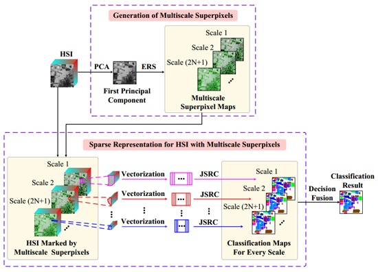
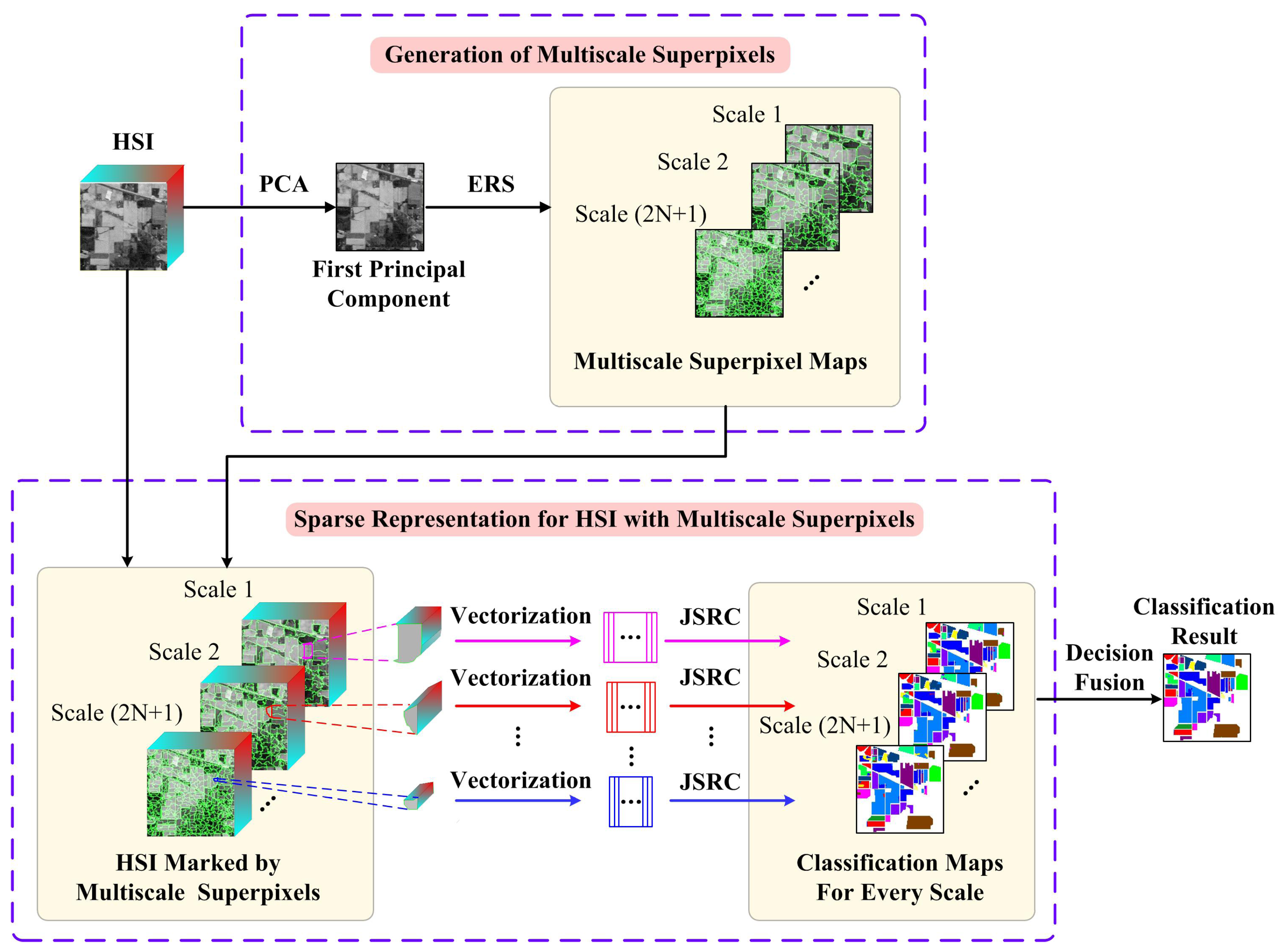
Figure 1.
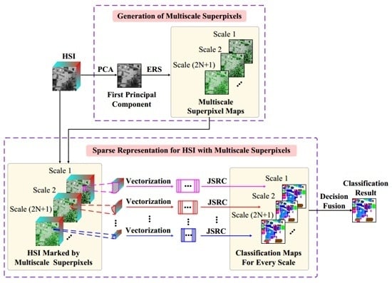
Schematic illustration of the multiscale superpixel-based sparse representation (MSSR) algorithm for HSI classification.
Figure 1.
Schematic illustration of the multiscale superpixel-based sparse representation (MSSR) algorithm for HSI classification.
Figure 2.
Indian Pines image: (a) false-color image; and (b) reference image.
Figure 2.
Indian Pines image: (a) false-color image; and (b) reference image.
Figure 3.
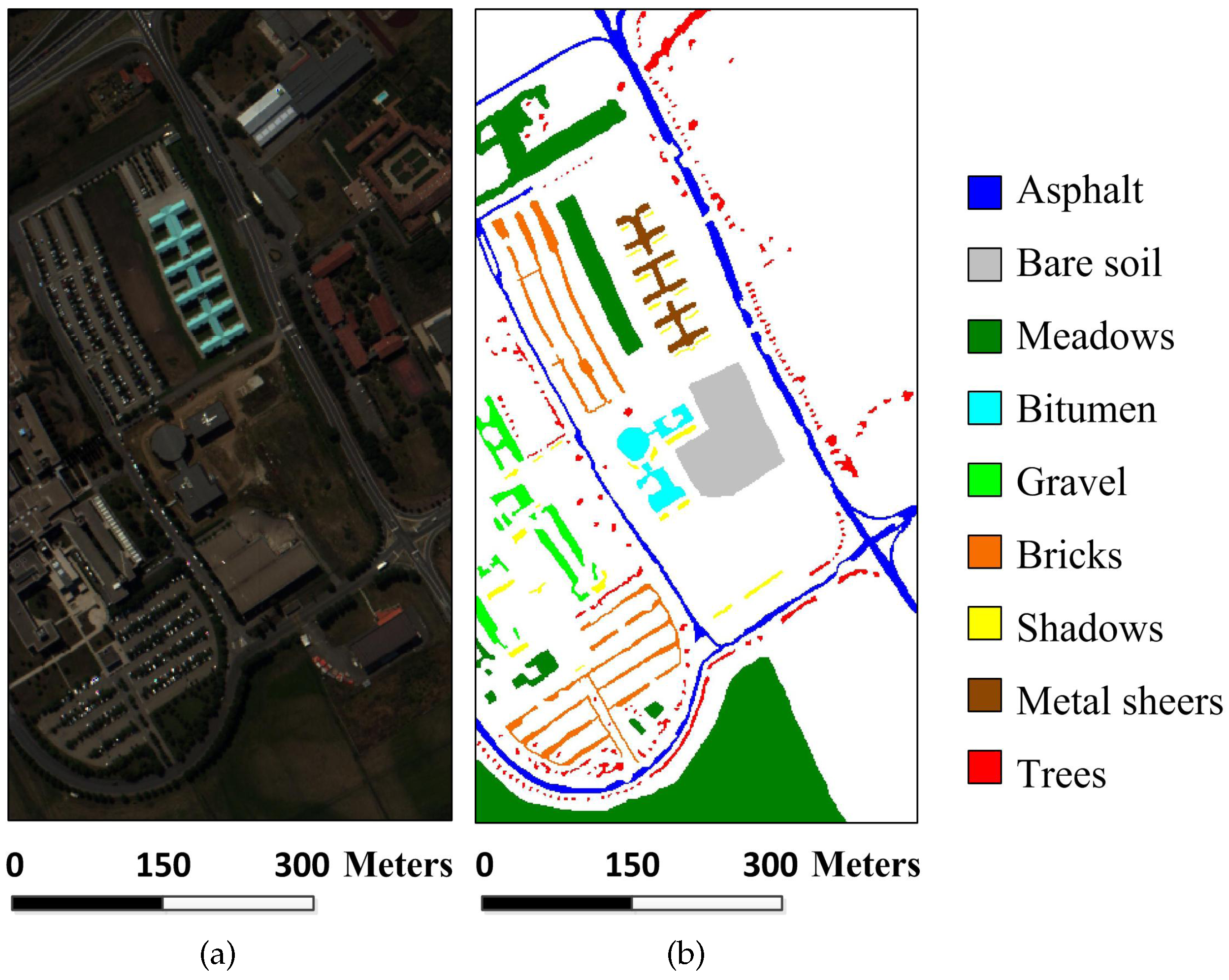
University of Pavia image: (a) false-color image; and (b) reference image.
Figure 3.
University of Pavia image: (a) false-color image; and (b) reference image.
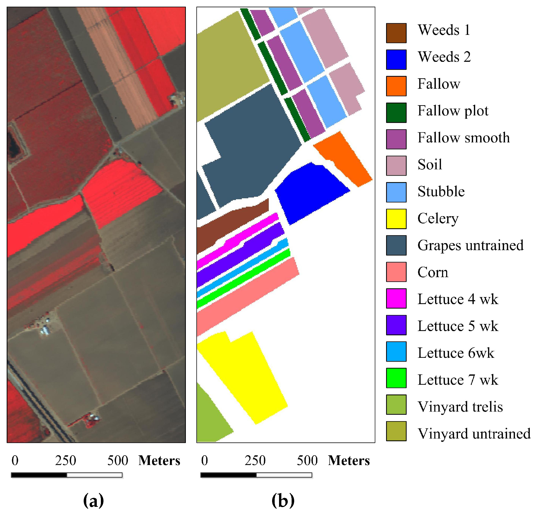
Figure 4.
Salinas image: (a) false-color image; and (b) reference image.
Figure 4.
Salinas image: (a) false-color image; and (b) reference image.
Figure 5.
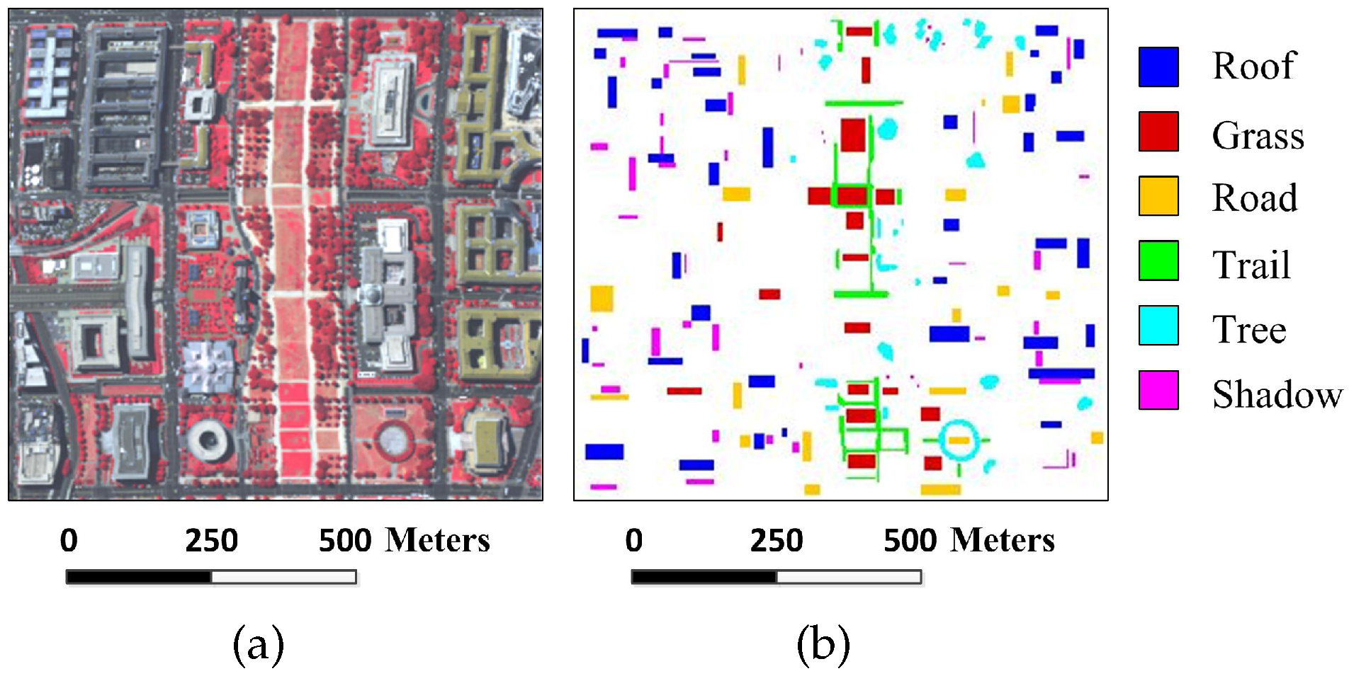
Washington DC image: (a) false-color image; and (b) reference image.
Figure 5.
Washington DC image: (a) false-color image; and (b) reference image.
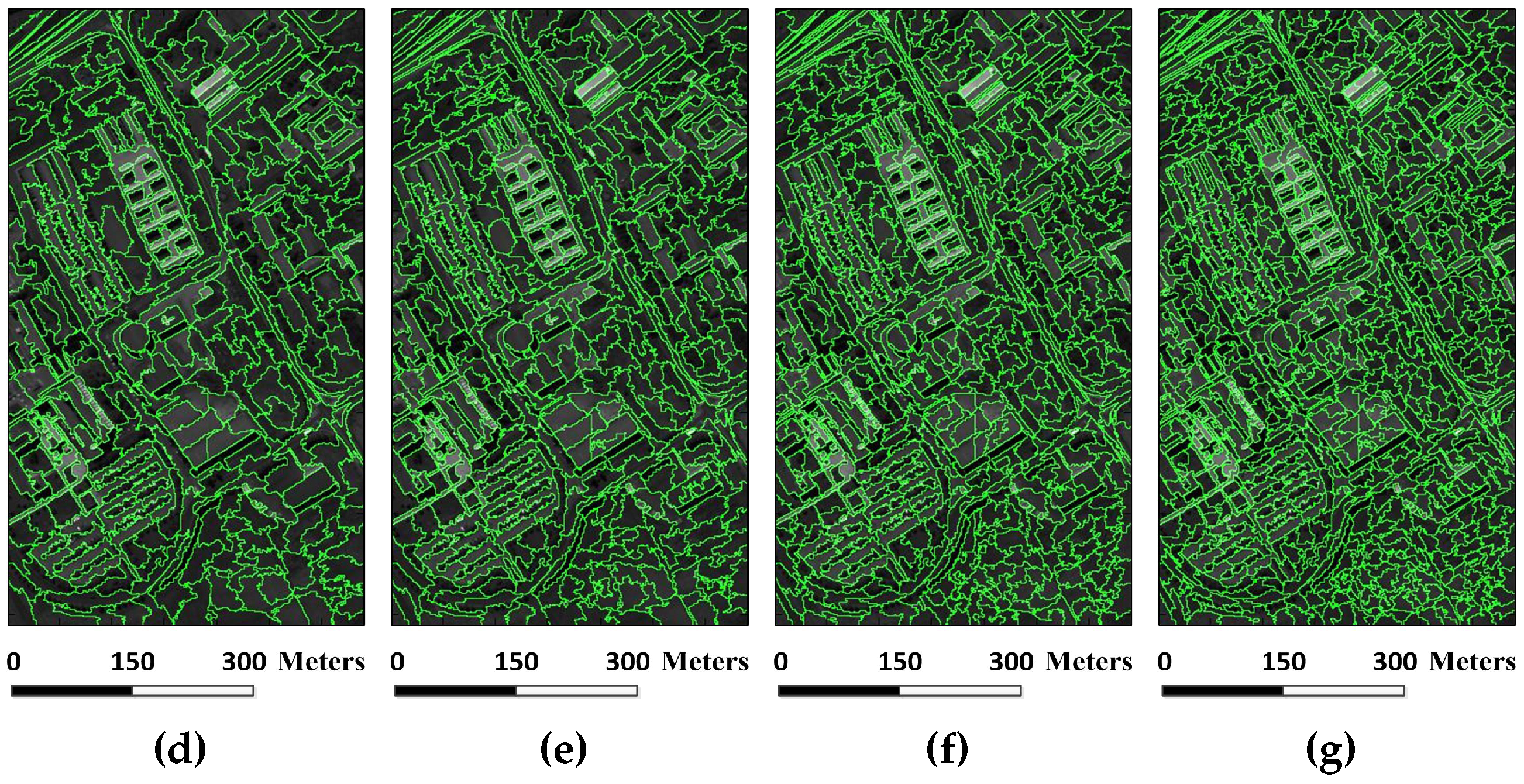
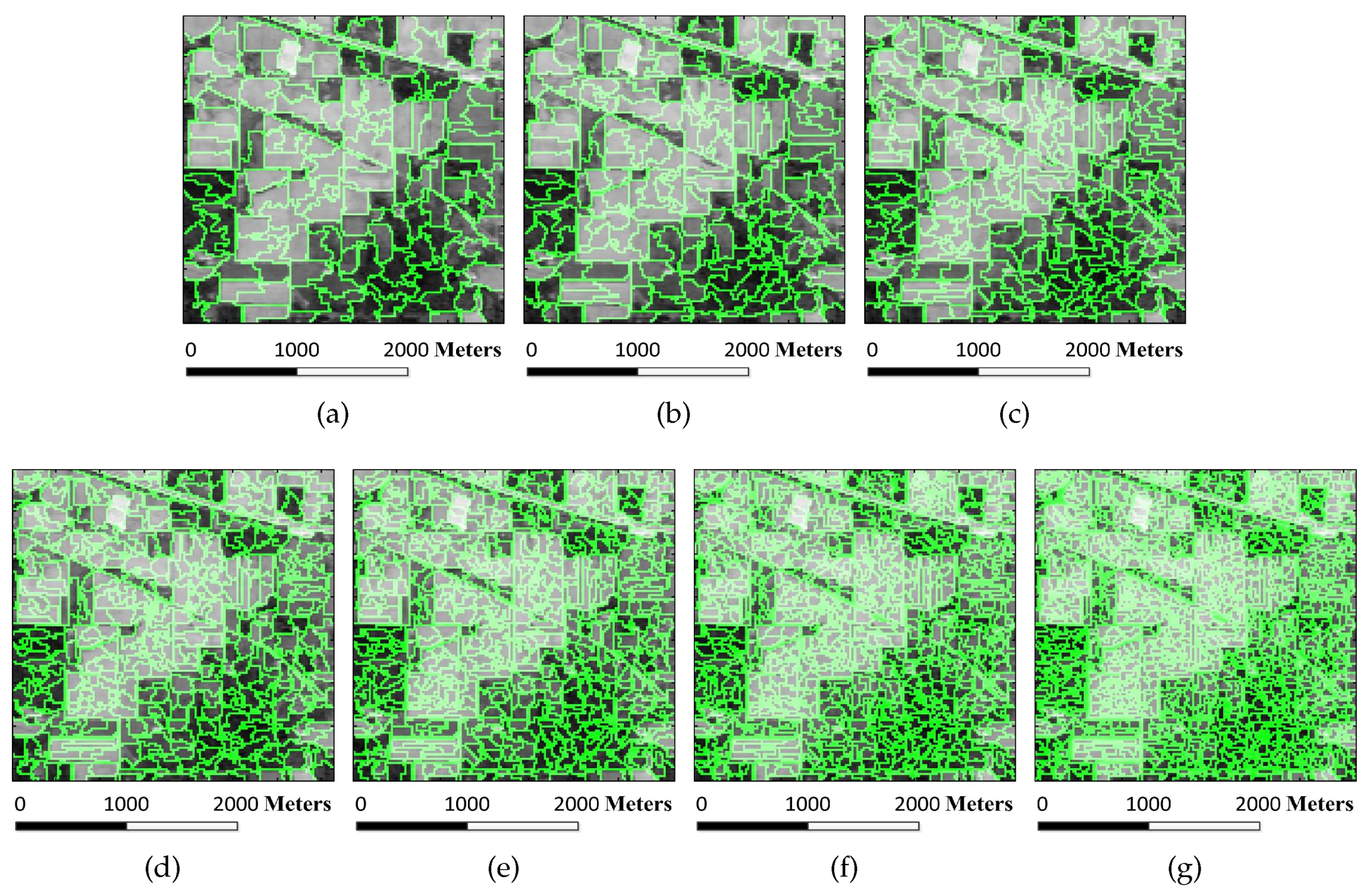
Figure 6.
Superpixel segmentation results of the Indian Pines image under different scales. The number of single-scale superpixels is gained by using the Equation (
5), in which the fundamental superpixel number is set to 3200 and the power exponent
n is an integer changing from
to three: (
a)
; (
b)
; (
c)
; (
d)
; (
e)
; (
f)
; and (
g)
.
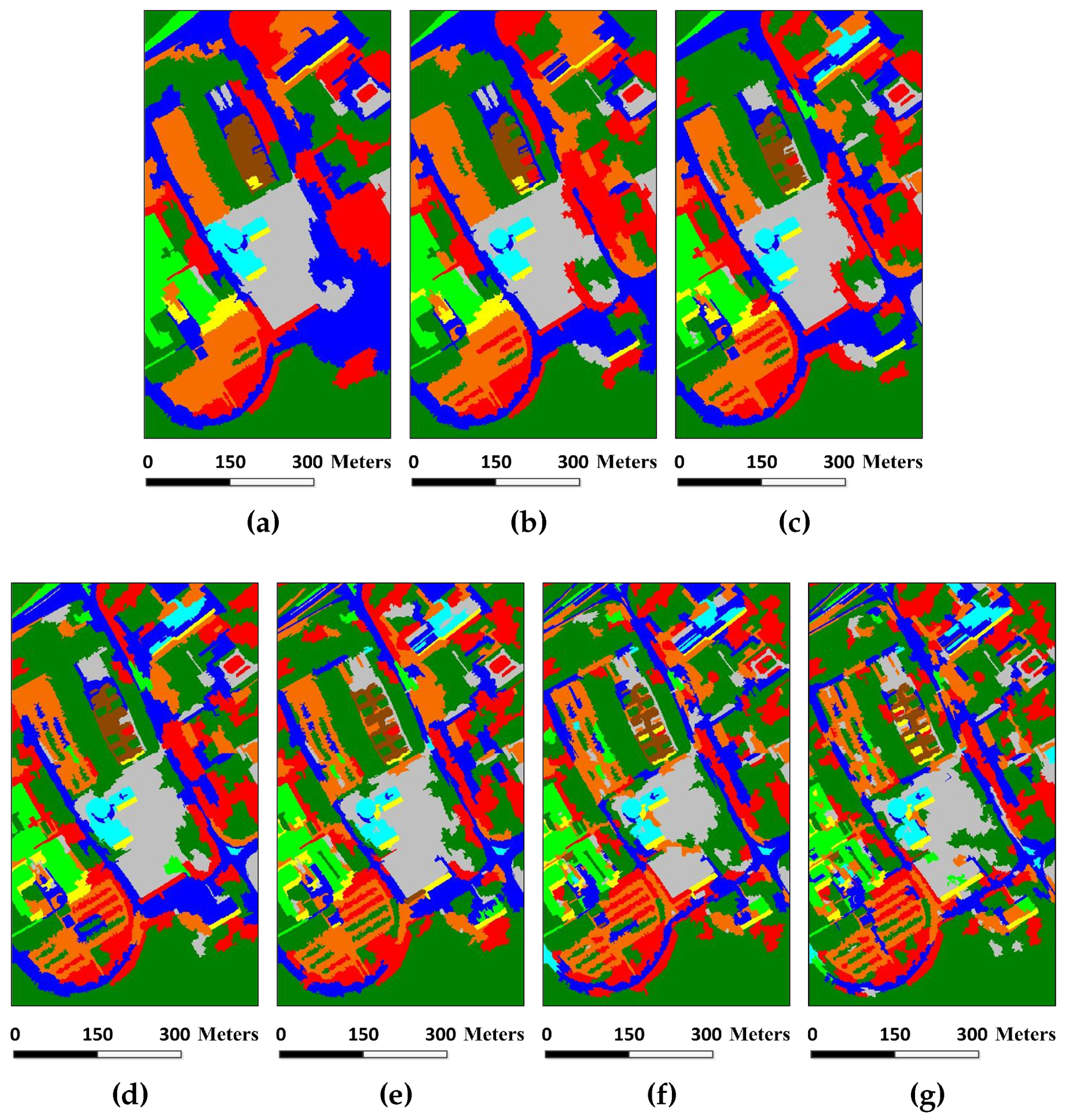
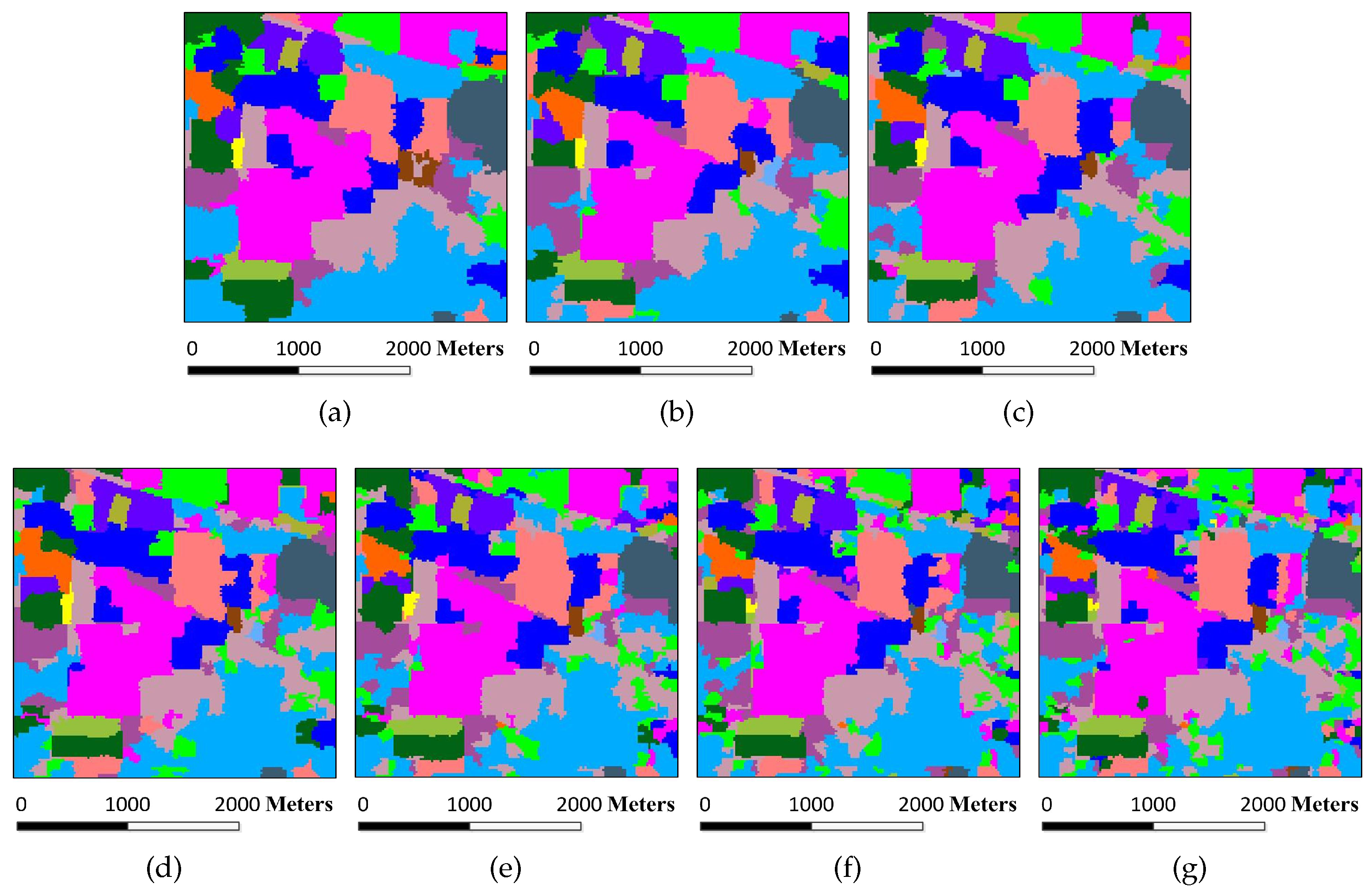
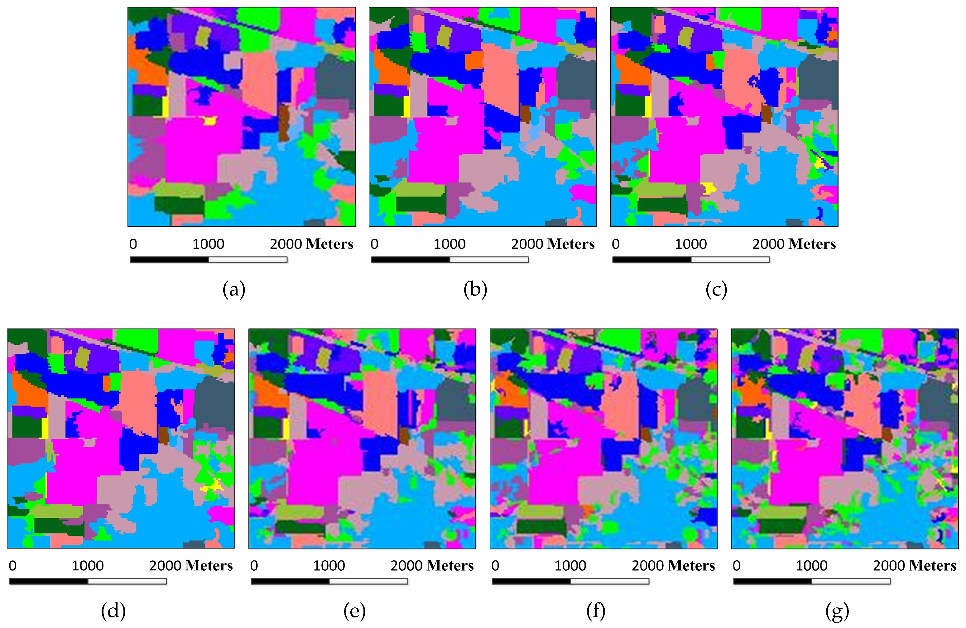
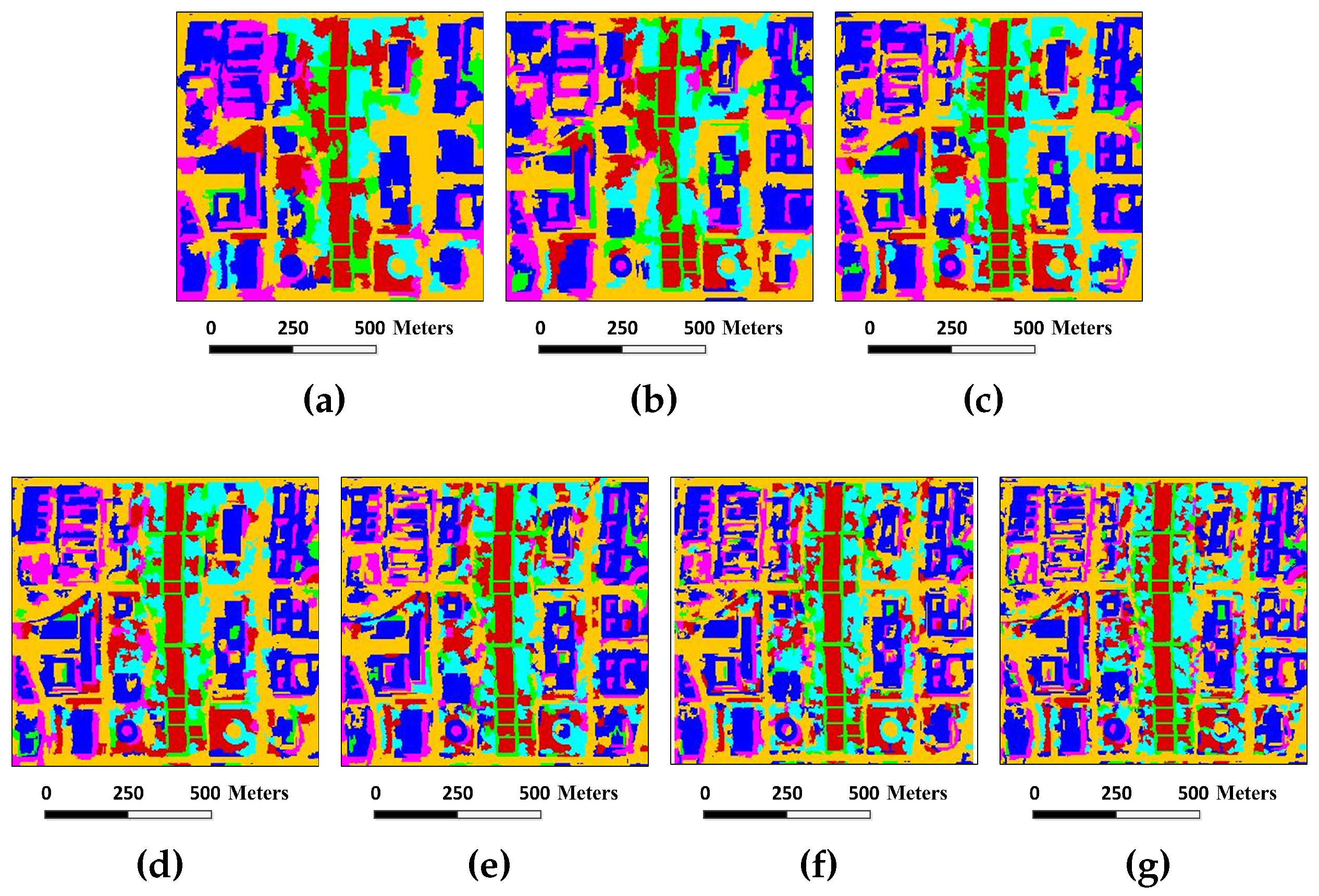
Figure 7.
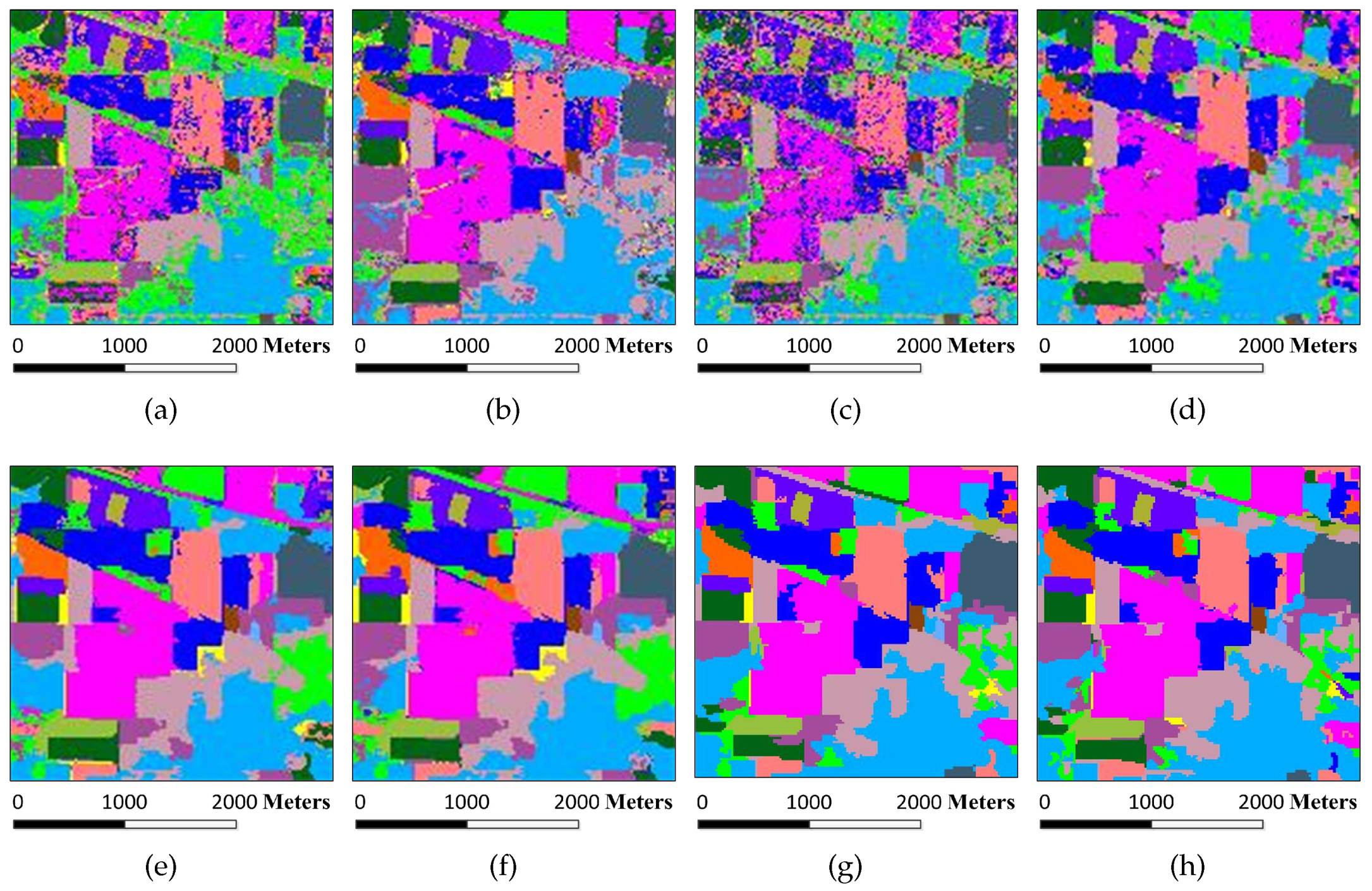
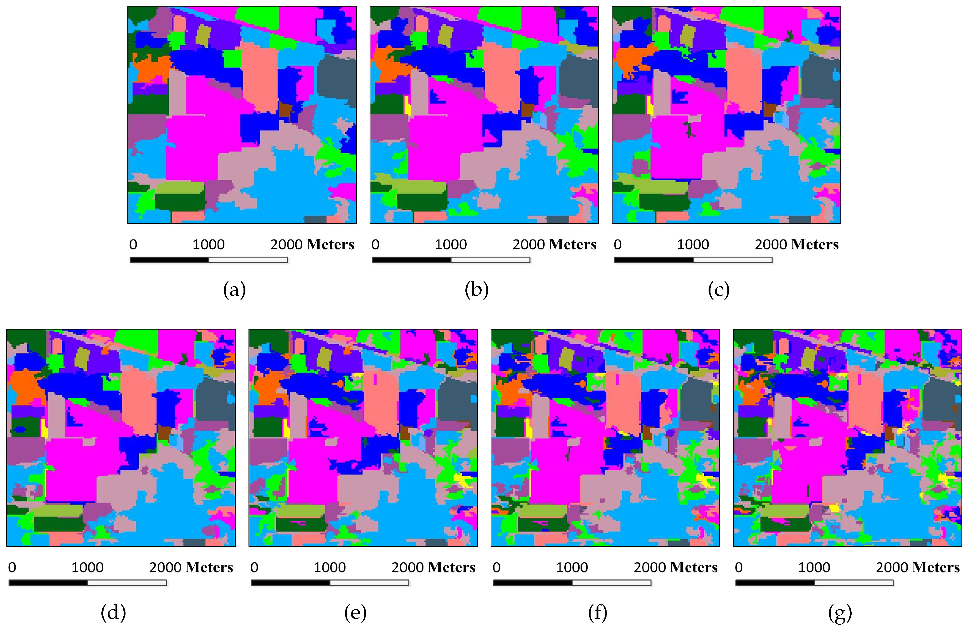
Classification results of the Indian Pines image under different scales. The number of single-scale superpixels is gained by using Equation (
5), in which the fundamental superpixel number is set to 3200 and the power exponent
n is an integer changing from
to three: (
a)
, OA = 93.14%; (
b)
, OA = 96.42%; (
c)
, OA = 96.62%; (
d)
, OA = 97.08%; (
e)
, OA = 95.64%; (
f)
, OA = 95.61%; and (
g)
, OA = 93.65%.
Figure 7.
Classification results of the Indian Pines image under different scales. The number of single-scale superpixels is gained by using Equation (
5), in which the fundamental superpixel number is set to 3200 and the power exponent
n is an integer changing from
to three: (
a)
, OA = 93.14%; (
b)
, OA = 96.42%; (
c)
, OA = 96.62%; (
d)
, OA = 97.08%; (
e)
, OA = 95.64%; (
f)
, OA = 95.61%; and (
g)
, OA = 93.65%.
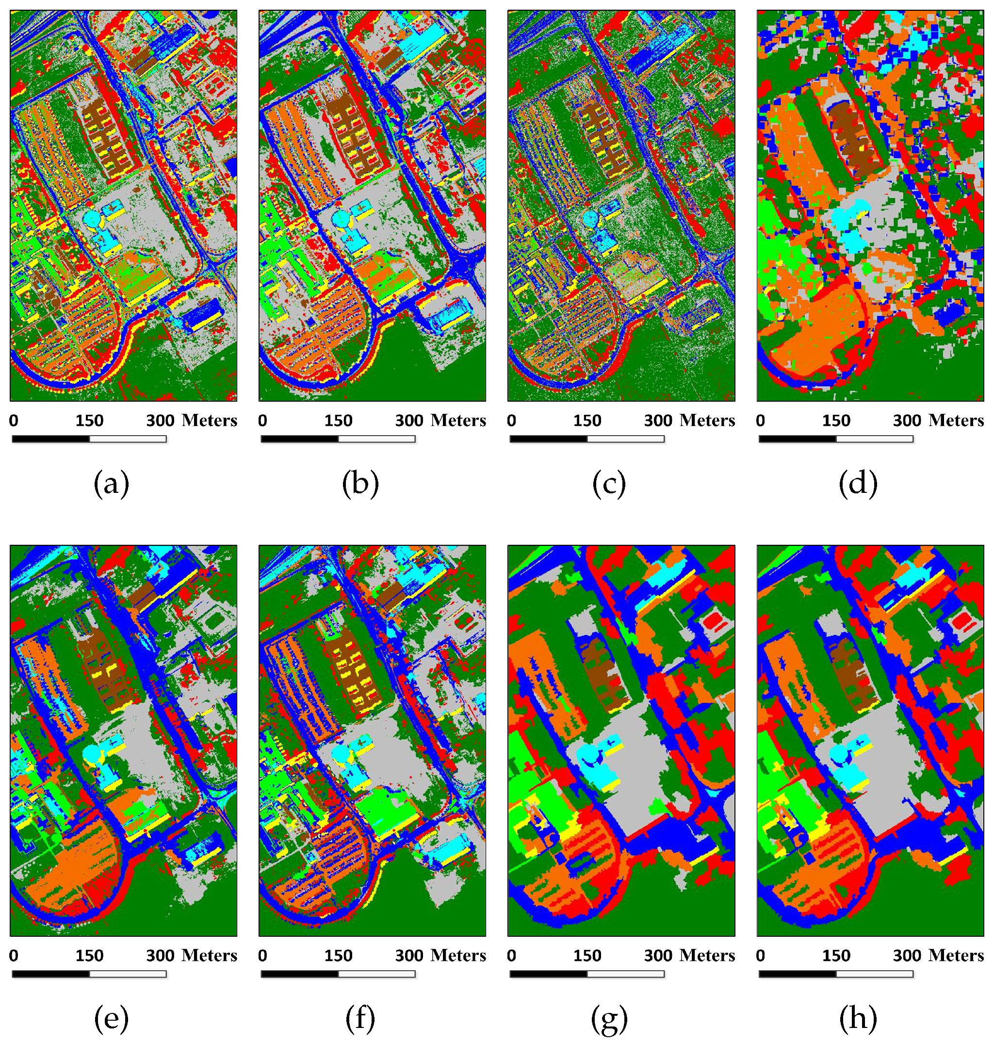
Figure 8.
Classification maps for the Indian Pines image by different algorithms (OA values are reported in parentheses): (a) SVM (78.01%); (b) EMP (92.71%); (c) SRC (68.91%); (d) JSRC (94.42%); (e) MASR (98.27%); (f) SCMK (97.96%); (g) SBDSM (97.08%); and (h) MSSR (98.58%).
Figure 8.
Classification maps for the Indian Pines image by different algorithms (OA values are reported in parentheses): (a) SVM (78.01%); (b) EMP (92.71%); (c) SRC (68.91%); (d) JSRC (94.42%); (e) MASR (98.27%); (f) SCMK (97.96%); (g) SBDSM (97.08%); and (h) MSSR (98.58%).
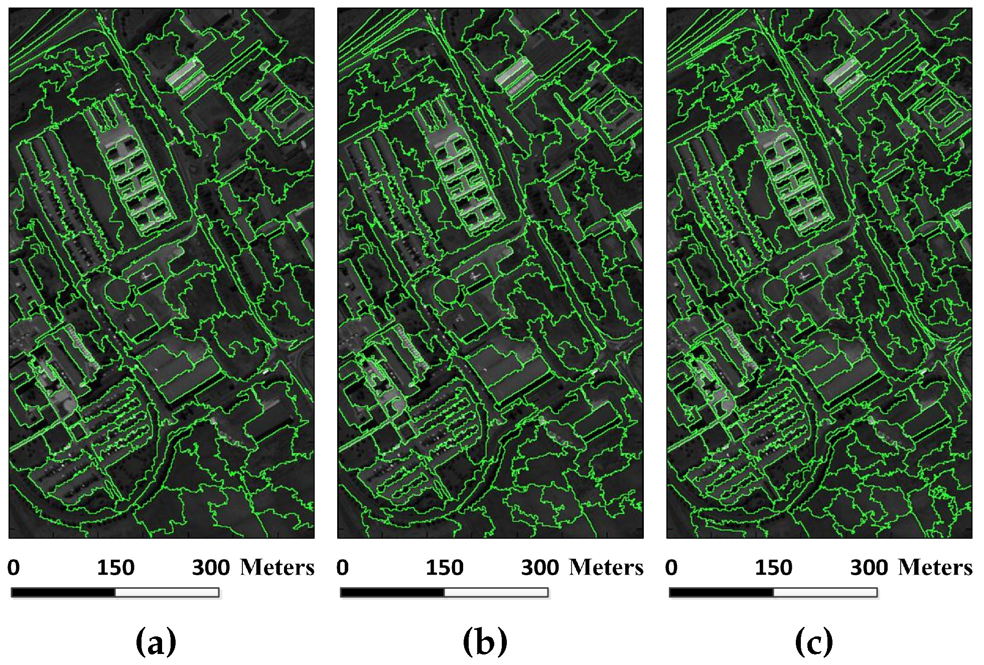
Figure 9.
Superpixel segmentation results of the University of Pavia image under different scales. The number of single-scale superpixels is gained by using Equation (
5), in which the fundamental superpixel number is set to 3200 and the power exponent
n is an integer changing from
to three: (
a)
; (
b)
; (
c)
; (
d)
; (
e)
; (
f)
; and (
g)
.
Figure 10.
Classification results of the University of Pavia image under different scales. The number of single-scale superpixels is gained by using Equation (
5), in which the fundamental superpixel number is set to 3200 and the power exponent
n is an integer changing from
to three: (
a)
, OA = 91.74%; (
b)
, OA = 91.42%; (
c)
, OA = 92.39%; (
d)
, OA = 92.60%; (
e)
, OA = 92.12%; (
f)
, OA = 91.54%; and (
g)
, OA = 91.35%.
Figure 11.
Classification maps for the Pavia University image by different algorithms (OA values are reported in parentheses): (a) SVM (86.52%); (b) EMP (91.80%); (c) SRC (77.90%); (d) JSRC (86.78%); (e) MASR (89.45%); (f) SCMK (94.96%); (g) SBDSM (92.60%); and (h) MSSR (95.47%).
Figure 11.
Classification maps for the Pavia University image by different algorithms (OA values are reported in parentheses): (a) SVM (86.52%); (b) EMP (91.80%); (c) SRC (77.90%); (d) JSRC (86.78%); (e) MASR (89.45%); (f) SCMK (94.96%); (g) SBDSM (92.60%); and (h) MSSR (95.47%).
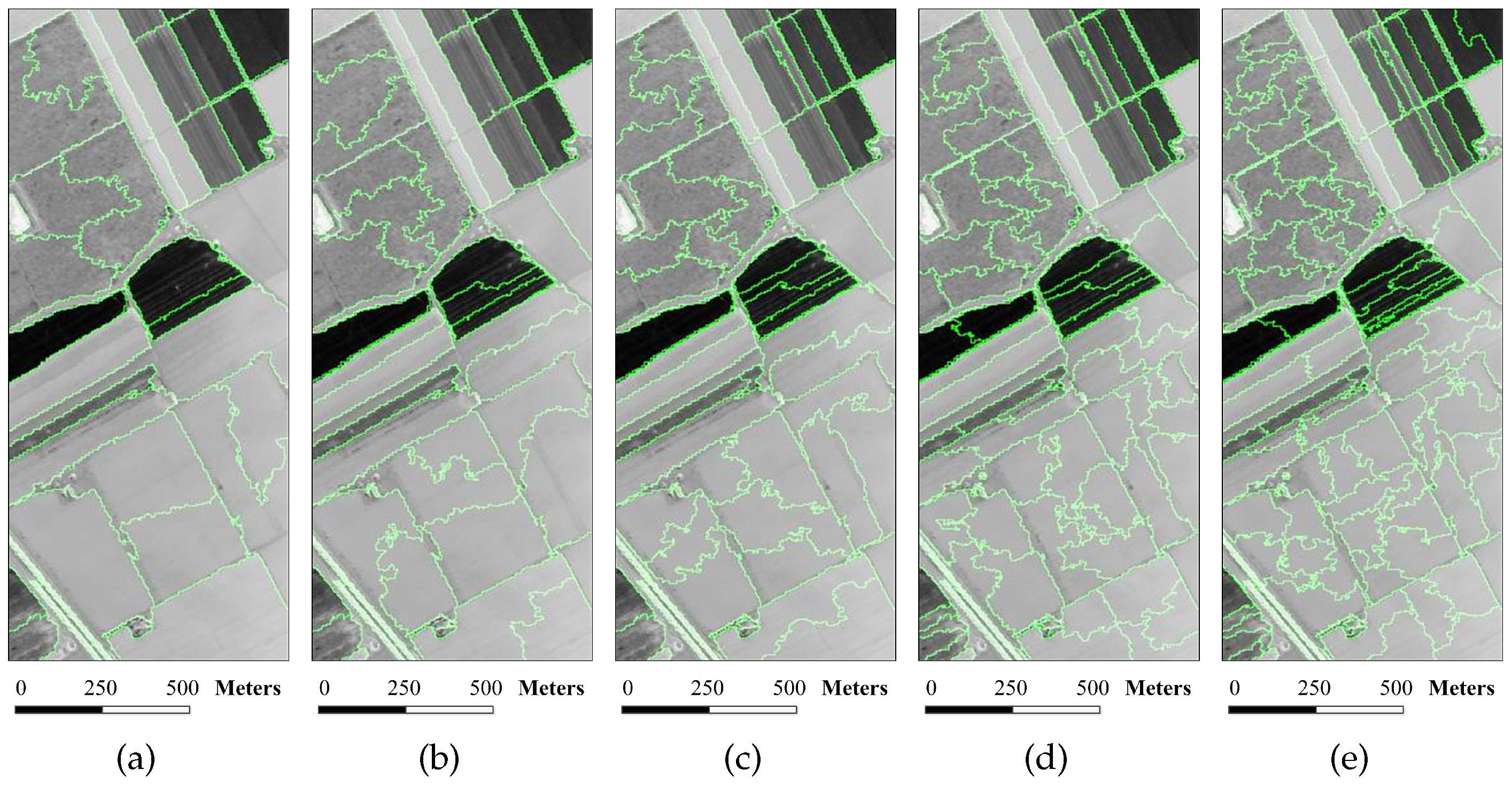
Figure 12.
Superpixel segmentation results of the Salinas image under different scales. The number of single-scale superpixels is gained by using Equation (
5), in which the fundamental superpixel number is set to 1600 and the power exponent
n is an integer changing from
to two: (
a)
; (
b)
; (
c)
; (
d)
; and (
e)
.
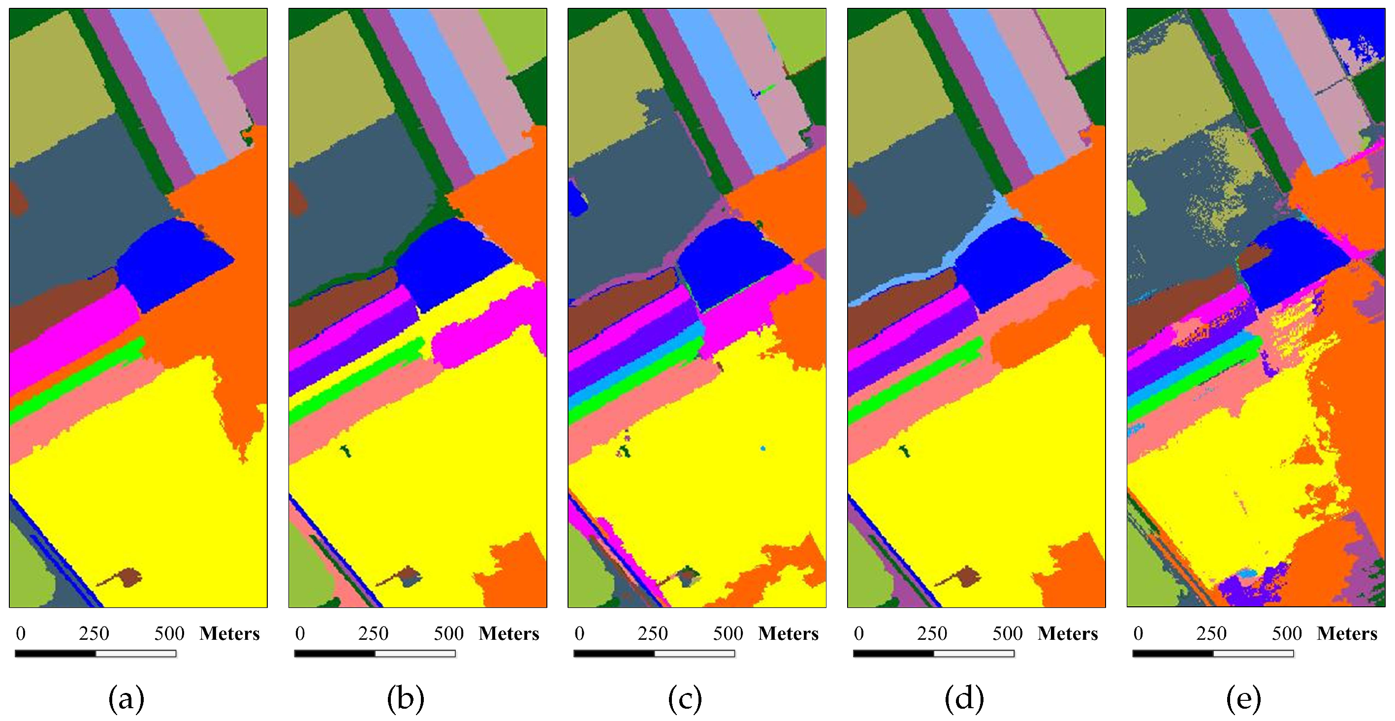
Figure 13.
Classification results of the Salinas image under different scales. The number of single-scale superpixels is gained by using Equation (
5), in which the fundamental superpixel number is set to 1600 and the power exponent
n is an integer changing from
to two: (
a)
, OA = 95.21%; (
b)
, OA = 97.04%; (
c)
, OA = 98.38%; (
d)
, OA = 97.70%; and (
e)
, OA = 97.00%.
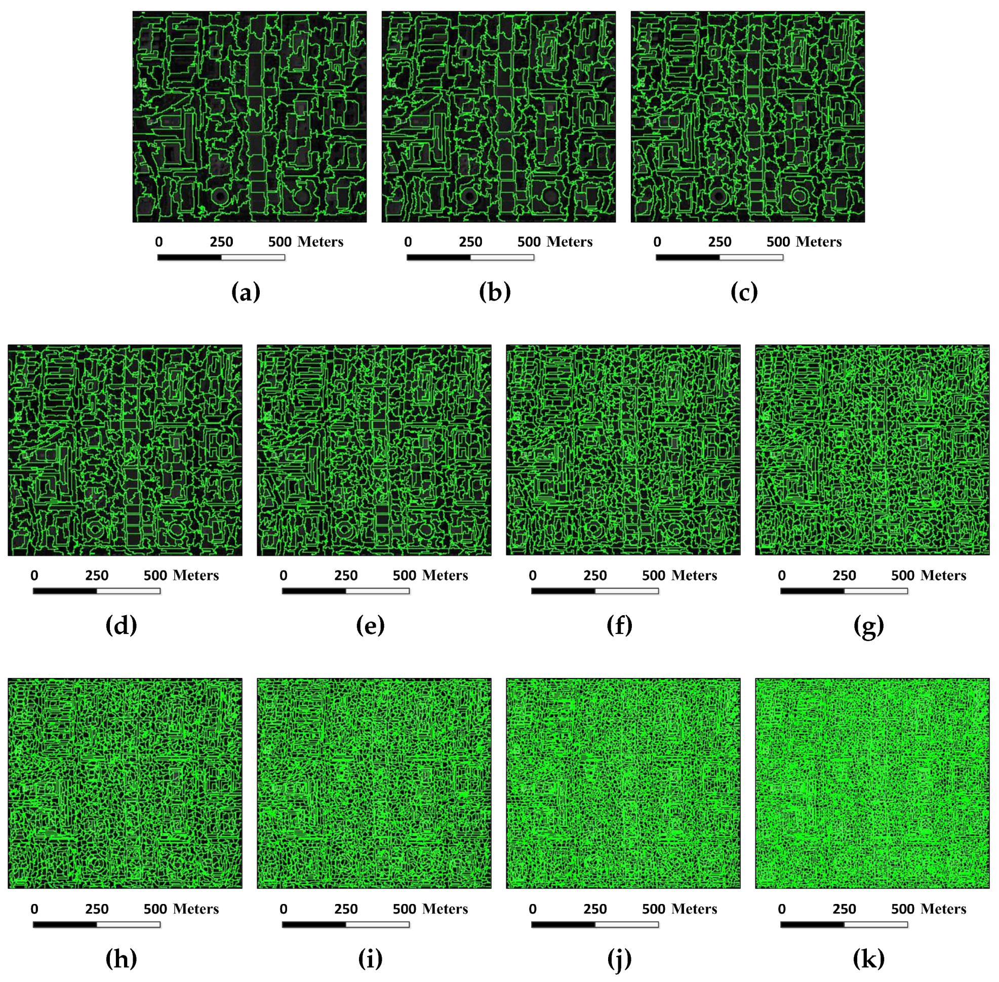
Figure 14.
Superpixel segmentation results of the Washington DC image under different scales. The number of single-scale superpixels is gained by using Equation (
5), in which the fundamental superpixel number is set to 12,800 and the power exponent
n is an integer changing from
to five: (
a)
; (
b)
; (
c)
; (
d)
; (
e)
; (
f)
; (
g)
; (
h)
; (
i)
; (
j)
; and (
k)
.
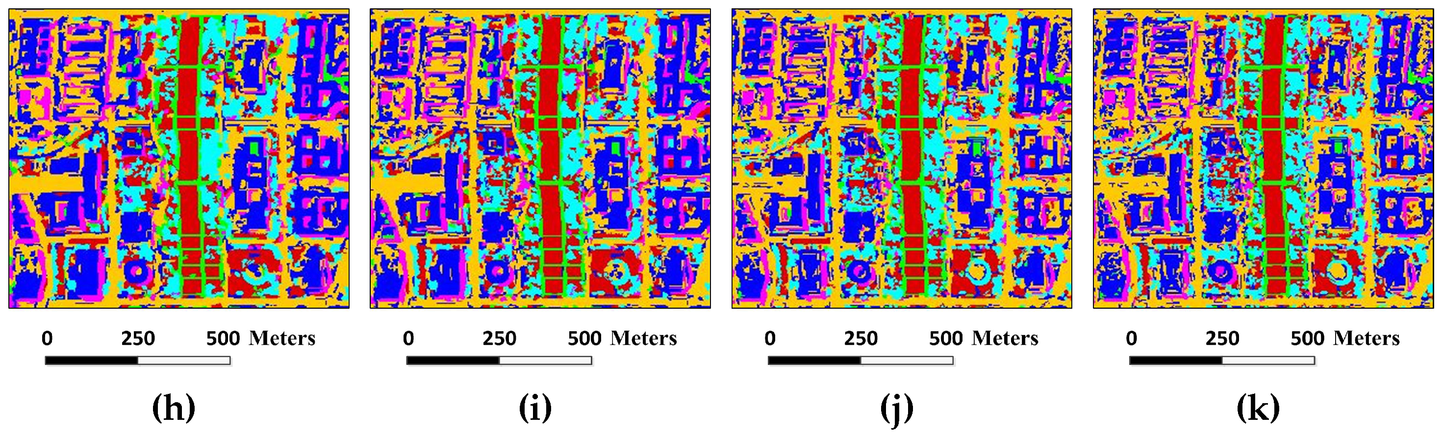
Figure 15.
Classification results of the Washington DC image under different scales. The number of single-scale superpixel is gained by using Equation (
5), in which the fundamental superpixel number is set to 12,800 and the power exponent
n is an integer changing from
to five: (
a)
, OA = 86.48%; (
b)
, OA = 90.29%; (
c)
, OA = 92.56%; (
d)
, OA = 91.43%; (
e)
, OA = 91.84%; (
f)
, OA = 93.33%; (
g)
, OA = 92.25%; (
h)
, OA = 92.49%; (
i)
, OA = 93.12%; (
j)
, OA = 92.55%; and (
k)
, OA = 92.31%.
Figure 16.
Classification maps for the Salinas image by different algorithms (OA values are reported in parentheses): (a) SVM (80.23%); (b) EMP (85.84%); (c) SRC (81.94%); (d) JSRC (84.79%); (e) MASR (92.21%); (f) SCMK (94.53%); (g) SBDSM (98.38%); and (h) MSSR (99.41%).
Figure 16.
Classification maps for the Salinas image by different algorithms (OA values are reported in parentheses): (a) SVM (80.23%); (b) EMP (85.84%); (c) SRC (81.94%); (d) JSRC (84.79%); (e) MASR (92.21%); (f) SCMK (94.53%); (g) SBDSM (98.38%); and (h) MSSR (99.41%).
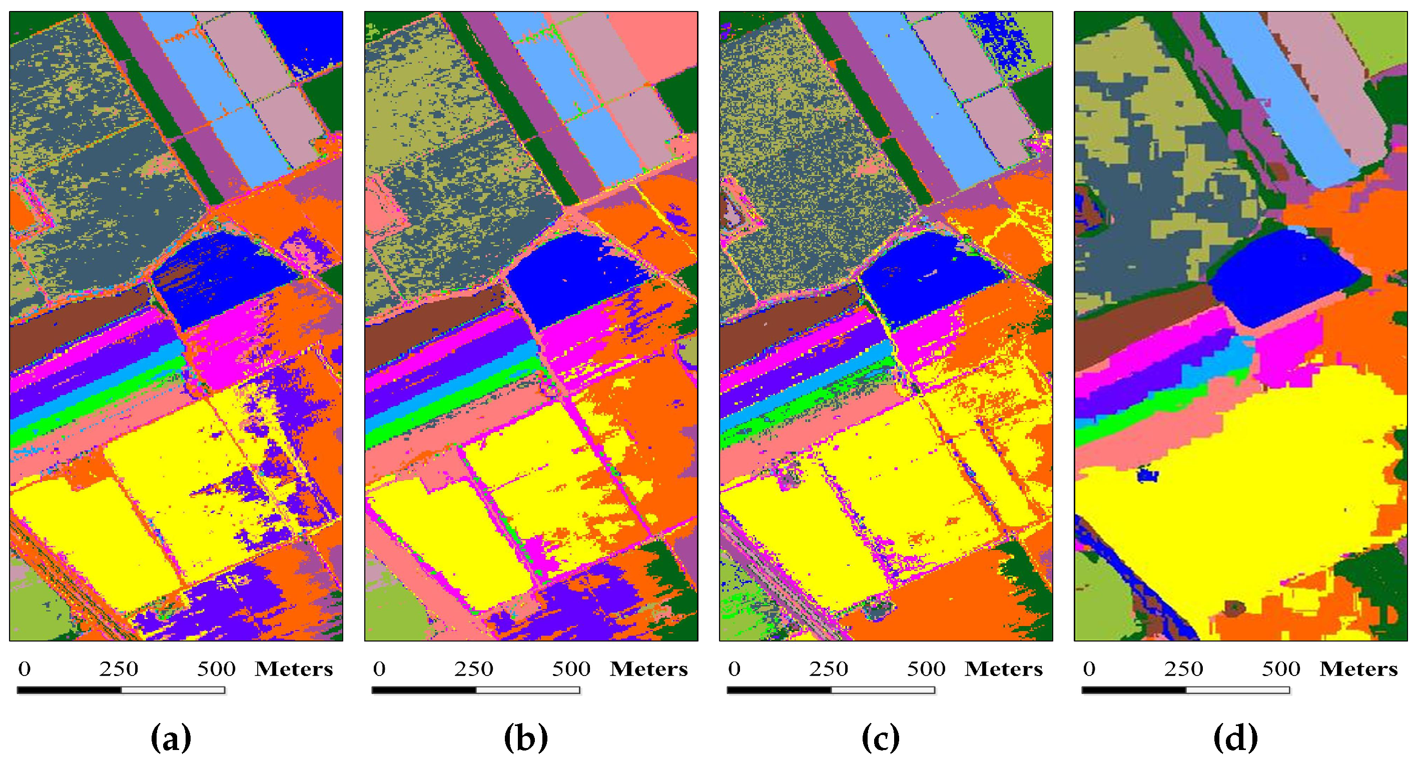
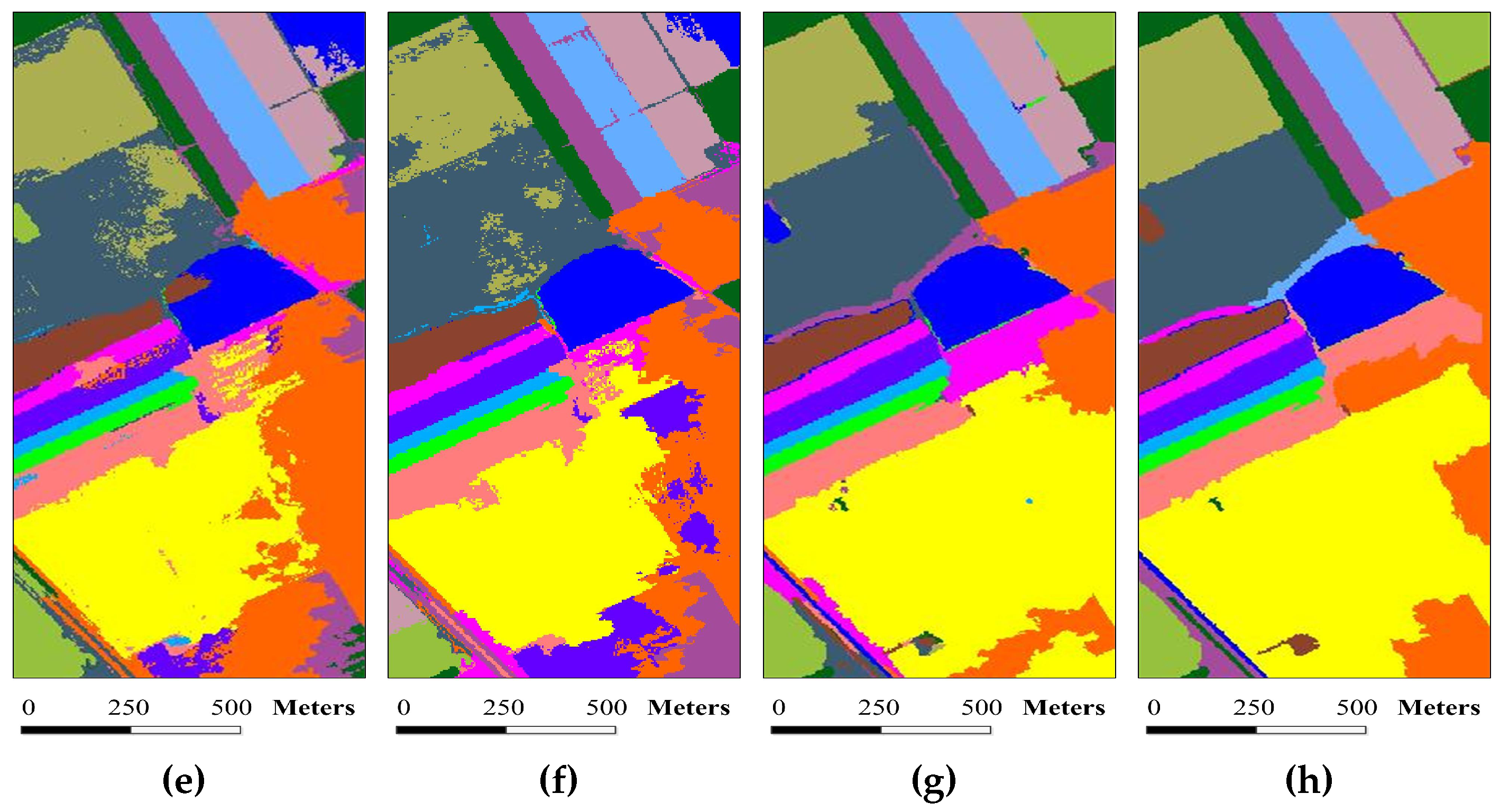
Figure 17.
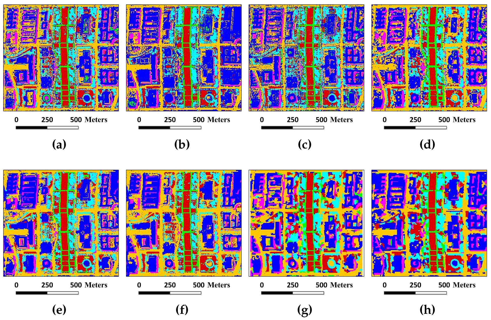
Classification maps for the Washington DC image by different algorithms (OA values are reported in parentheses): (a) SVM (90.98%); (b) EMP (90.28%); (c) SRC (91.95%); (d) JSRC (92.79%); (e) MASR (95.62%); (f) SCMK (94.55%); (g) SBDSM (93.33%); and(h) MSSR (96.60%).
Figure 17.
Classification maps for the Washington DC image by different algorithms (OA values are reported in parentheses): (a) SVM (90.98%); (b) EMP (90.28%); (c) SRC (91.95%); (d) JSRC (92.79%); (e) MASR (95.62%); (f) SCMK (94.55%); (g) SBDSM (93.33%); and(h) MSSR (96.60%).
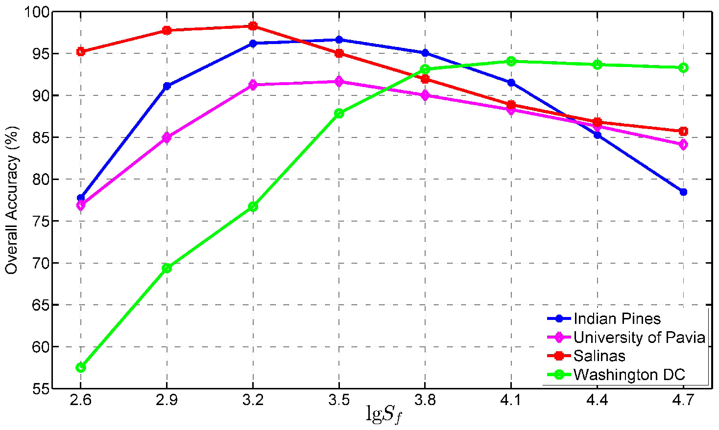
Figure 18.
Classification accuracy OA versus different fundamental superpixel numbers on the four test images.
Figure 18.
Classification accuracy OA versus different fundamental superpixel numbers on the four test images.
Figure 19.
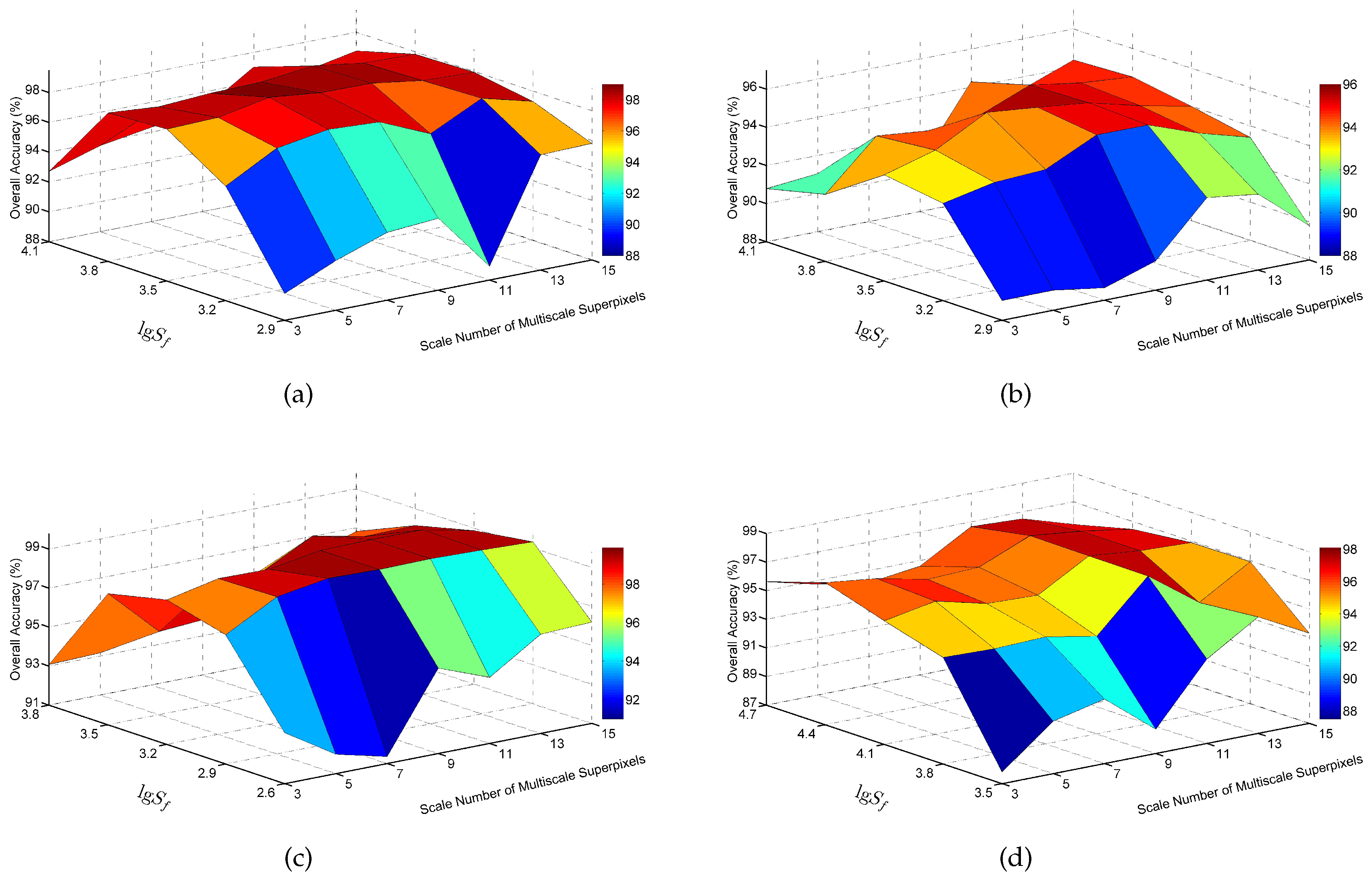
Relationship among the OA value, the number of multiscale superpixels and the fundamental superpixel number : (a) Indian Pines image; (b) University of Pavia image; (c) Salinas image; and (d) Washington DC image.
Figure 19.
Relationship among the OA value, the number of multiscale superpixels and the fundamental superpixel number : (a) Indian Pines image; (b) University of Pavia image; (c) Salinas image; and (d) Washington DC image.
Figure 20.
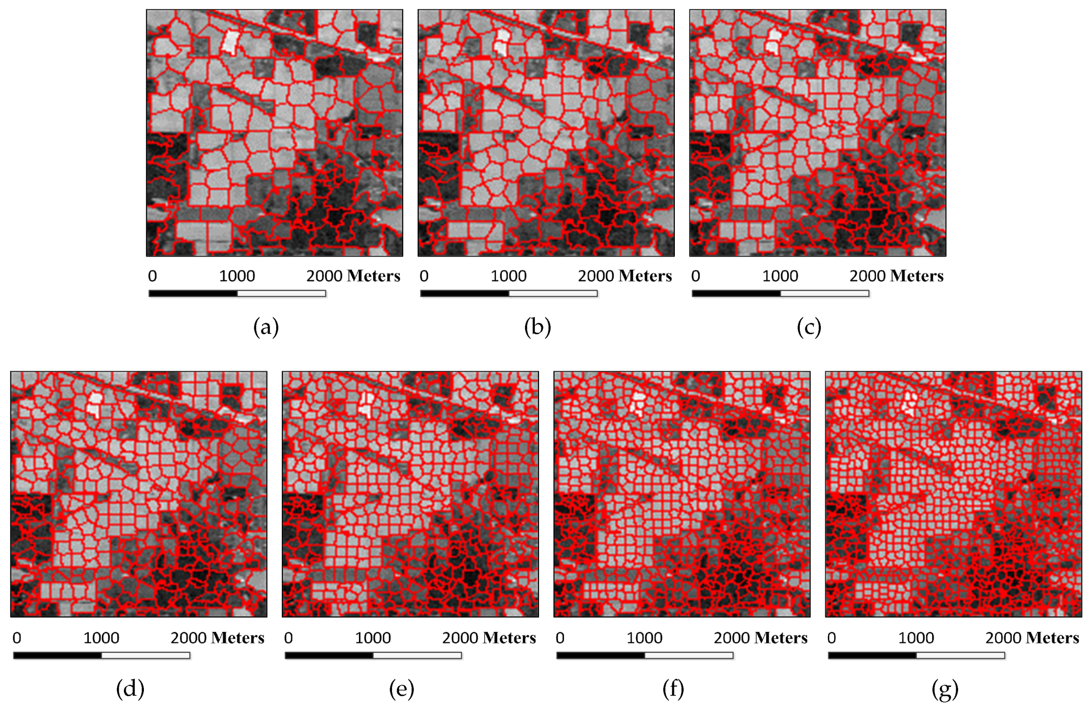
Felzenszwalb-Huttenlocher (FH) segmentation results of the Indian Pines image under different scales. Multiscale superpixels are generated with various scales and smoothing parameters, σ and : (a) ; (b) ; (c) ; (d) ; (e) ; (f) ; and (g) .
Figure 20.
Felzenszwalb-Huttenlocher (FH) segmentation results of the Indian Pines image under different scales. Multiscale superpixels are generated with various scales and smoothing parameters, σ and : (a) ; (b) ; (c) ; (d) ; (e) ; (f) ; and (g) .
Figure 21.
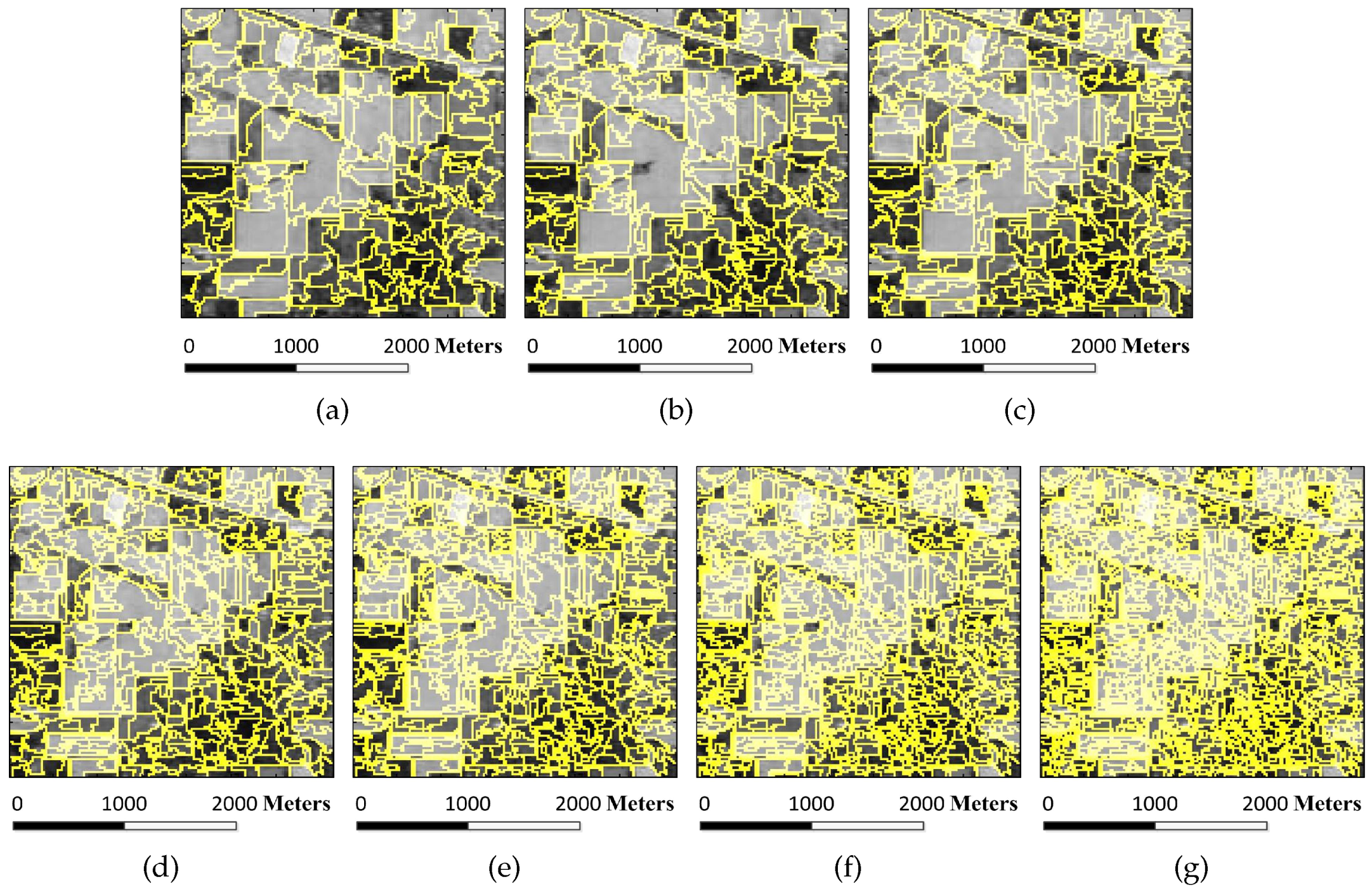
Simple linear iterative clustering (SLIC) segmentation results of the Indian Pines image under different scales. The number of multiscale superpixels is obtained by presetting the number of superpixel segmentations : (a) = 147; (b) = 206; (c) = 288; (d) = 415; (e) = 562; (f) = 780; and (g) = 1055.
Figure 21.
Simple linear iterative clustering (SLIC) segmentation results of the Indian Pines image under different scales. The number of multiscale superpixels is obtained by presetting the number of superpixel segmentations : (a) = 147; (b) = 206; (c) = 288; (d) = 415; (e) = 562; (f) = 780; and (g) = 1055.
Figure 22.
Classification results of the Indian Pines image under different scales. The FH segmentation method is applied in the SBDSM algorithm. Multiscale superpixels are generated with various scales and smoothing parameters, σ and : (a) , OA = 83.56%; (b) , OA = 93.21%; (c) , OA = 93.52%; (d) , OA = 96.25%; (e) , OA = 94.52%; (f) , OA = 94.32%; and (g) , OA = 94.28%.
Figure 23.
Classification results of the Indian Pines image under different scales. The SLIC segmentation method is applied in the SBDSM algorithm. The number of multiscale superpixels is obtained by presetting the number of superpixel segmentations : (a) = 147, OA = 89.10%; (b) = 206, OA = 91.45%; (c) = 288, OA = 93.16%; (d) = 415, OA = 96.81%; (e) = 562, OA = 96.52%; (f) = 780, OA = 95.32%; and (g) = 1055, OA = 95.24%.
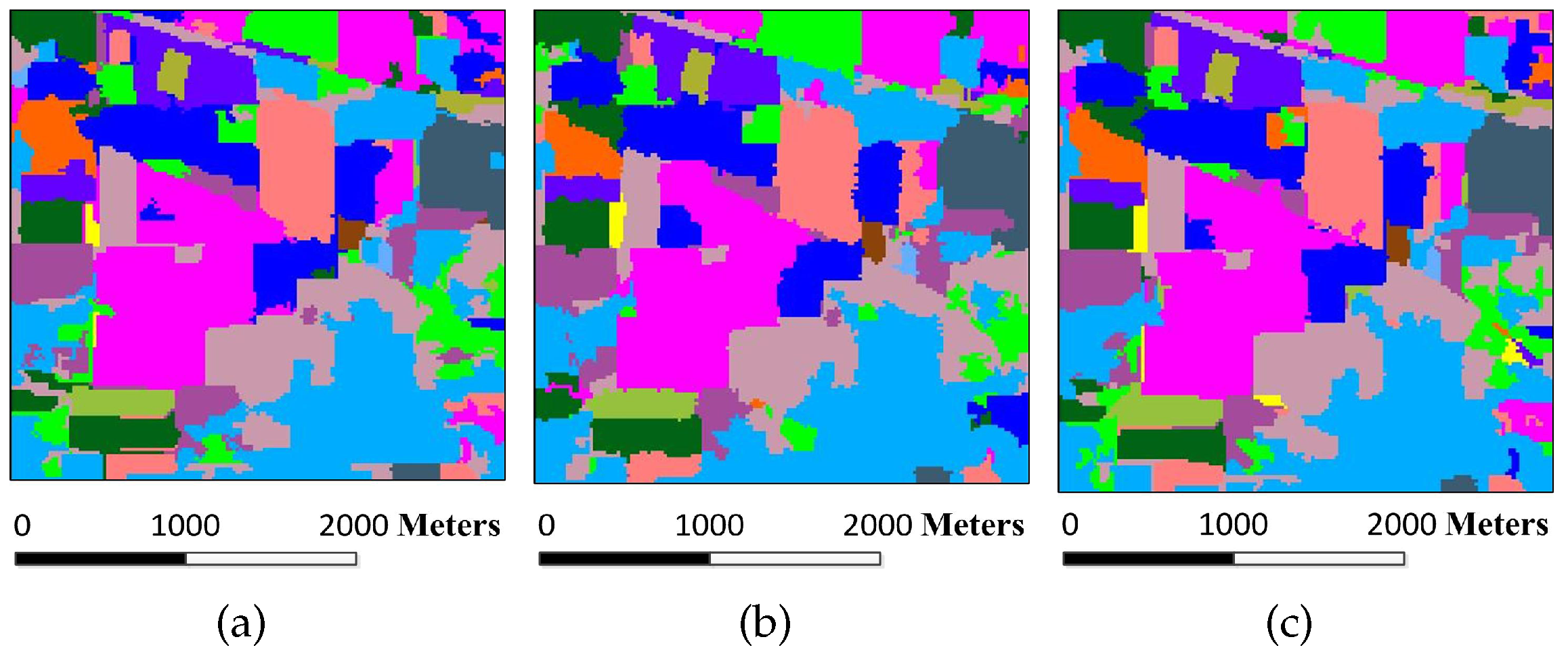
Figure 24.
Classification maps by using MSSR_FH, MSSR_SLIC and MSSR_ERS algorithms: (a) MSSR_FH, OA = 96.54%; (b) MSSR_SLIC, OA = 97.38%; (c) MSSR_ERS, OA = 98.58%.
Figure 24.
Classification maps by using MSSR_FH, MSSR_SLIC and MSSR_ERS algorithms: (a) MSSR_FH, OA = 96.54%; (b) MSSR_SLIC, OA = 97.38%; (c) MSSR_ERS, OA = 98.58%.
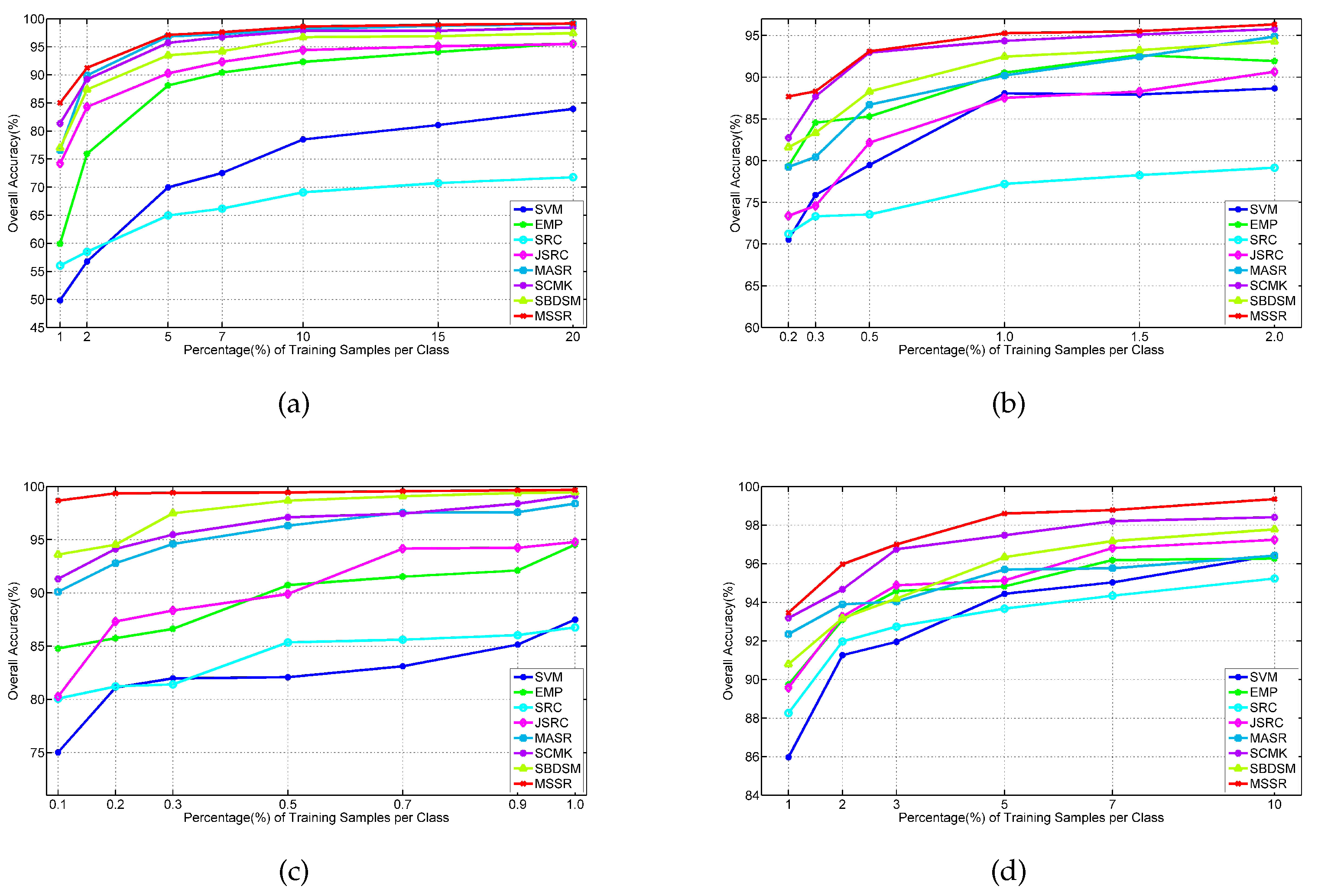
Figure 25.
Effect of the number of training samples on SVM, EMP, SRC, JSRC, MASR, SCMK, SBDSM and MSSR for the: (a) Indian Pines image; (b) University of Pavia images; (c) Salinas image; and (d) Washington DC image.
Figure 25.
Effect of the number of training samples on SVM, EMP, SRC, JSRC, MASR, SCMK, SBDSM and MSSR for the: (a) Indian Pines image; (b) University of Pavia images; (c) Salinas image; and (d) Washington DC image.
Table 1.
Number of training and test samples of sixteen classes in the Indian Pines image.
Table 1.
Number of training and test samples of sixteen classes in the Indian Pines image.
| Class | Name | Train | Test |
|---|
| 1 | Alfalfa | 5 | 41 |
| 2 | Corn-no till | 143 | 1285 |
| 3 | Corn-min till | 83 | 747 |
| 4 | Corn | 24 | 213 |
| 5 | Grass/pasture | 49 | 434 |
| 6 | Grass/tree | 73 | 657 |
| 7 | Grass/pasture-mowed | 3 | 25 |
| 8 | Hay-windrowed | 48 | 430 |
| 9 | Oats | 2 | 18 |
| 10 | Soybean-no till | 98 | 874 |
| 11 | Soybean-min till | 246 | 2209 |
| 12 | Soybean-clean till | 60 | 533 |
| 13 | Wheat | 21 | 184 |
| 14 | Woods | 127 | 1138 |
| 15 | Bldg-grass-trees-drives | 39 | 347 |
| 16 | Stone-steel towers | 10 | 83 |
| | Total | 1031 | 9218 |
Table 2.
Classification accuracy of the Indian Pines image under different scales. The number of single-scale superpixels is gained by using Equation (
5), in which the fundamental superpixel number is set to 3200 and the power exponent
n is an integer changing from
to three. Class-specific accuracy values are in percentage. The best results are highlighted in bold typeface. AA, average accuracy.
Table 2.
Classification accuracy of the Indian Pines image under different scales. The number of single-scale superpixels is gained by using Equation (5), in which the fundamental superpixel number is set to 3200 and the power exponent n is an integer changing from to three. Class-specific accuracy values are in percentage. The best results are highlighted in bold typeface. AA, average accuracy.
| Class | | | | | | | |
|---|
| 1 | 99.01 | 98.05 | 99.02 | 97.56 | 98.05 | 97.56 | 90.73 |
| 2 | 87.21 | 90.27 | 95.04 | 96.34 | 90.41 | 92.54 | 90.33 |
| 3 | 92.05 | 95.53 | 97.11 | 89.69 | 95.61 | 92.34 | 92.88 |
| 4 | 95.31 | 99.06 | 99.04 | 99.06 | 88.64 | 91.55 | 87.98 |
| 5 | 91.71 | 94.10 | 94.79 | 93.55 | 94.47 | 94.01 | 92.30 |
| 6 | 99.88 | 99.76 | 99.76 | 99.85 | 99.30 | 98.48 | 97.53 |
| 7 | 96.00 | 96.00 | 97.60 | 96.43 | 96.00 | 96.80 | 96.00 |
| 8 | 100 | 100 | 100 | 100 | 100 | 98.79 | 98.28 |
| 9 | 100 | 100 | 100 | 100 | 100 | 94.44 | 86.67 |
| 10 | 90.48 | 96.84 | 92.20 | 94.74 | 93.91 | 94.74 | 93.46 |
| 11 | 93.86 | 97.32 | 96.51 | 96.92 | 97.71 | 96.43 | 95.15 |
| 12 | 82.66 | 92.35 | 95.20 | 97.75 | 90.73 | 91.22 | 84.80 |
| 13 | 100 | 99.46 | 99.57 | 99.46 | 99.46 | 99.13 | 99.46 |
| 14 | 99.74 | 99.93 | 99.74 | 99.82 | 99.46 | 98.54 | 98.98 |
| 15 | 93.60 | 98.04 | 91.87 | 93.08 | 95.33 | 93.03 | 83.80 |
| 16 | 96.63 | 96.39 | 97.59 | 96.39 | 97.11 | 97.56 | 91.57 |
| OA (%) | 93.37 | 96.44 | 96.56 | 96.92 | 95.77 | 95.32 | 93.62 |
| AA (%) | 94.88 | 95.07 | 95.19 | 95.19 | 95.01 | 95.45 | 92.50 |
| Kappa | 0.92 | 0.95 | 0.95 | 0.95 | 0.95 | 0.95 | 0.93 |
Table 3.
Classification accuracy of the Indian Pines image by the classification algorithms used in this work for comparison. Class-specific accuracy values are in percentage. The best results are highlighted in bold typeface. EMP, extended morphological profile; JSRC, joint sparse representation classification; MASR, multiscale adaptive sparse representation; SCMK, superpixel-based classification via multiple kernel; SBDSM, superpixel-based discriminative sparse model; MSSR, multiscale superpixel-based sparse representation.
| Class | SVM | EMP | SRC | JSRC | MASR | SCMK | SBDSM | MSSR |
|---|
| 1 | 80.24 | 98.22 | 58.64 | 92.68 | 94.68 | 99.99 | 97.56 | 97.45 |
| 2 | 72.99 | 85.84 | 52.35 | 94.68 | 97.25 | 97.24 | 96.34 | 97.83 |
| 3 | 66.76 | 90.86 | 53.65 | 93.44 | 97.34 | 97.20 | 89.69 | 99.60 |
| 4 | 84.10 | 93.75 | 36.78 | 91.93 | 97.41 | 96.89 | 99.06 | 98.59 |
| 5 | 90.68 | 93.40 | 82.35 | 94.05 | 97.20 | 96.31 | 93.55 | 98.16 |
| 6 | 94.09 | 98.47 | 89.98 | 95.58 | 99.62 | 99.59 | 99.85 | 99.82 |
| 7 | 83.96 | 92.75 | 88.56 | 83.20 | 96.41 | 99.68 | 96.43 | 96.73 |
| 8 | 96.15 | 99.90 | 90.23 | 99.86 | 99.89 | 100 | 100 | 100 |
| 9 | 92.00 | 100 | 71.35 | 36.67 | 76.42 | 100 | 100 | 92.23 |
| 10 | 77.11 | 87.45 | 68.32 | 91.21 | 97.99 | 92.35 | 94.74 | 98.28 |
| 11 | 69.84 | 91.91 | 75.32 | 95.98 | 98.64 | 98.61 | 96.92 | 99.28 |
| 12 | 73.72 | 87.85 | 42.56 | 88.89 | 97.72 | 96.78 | 97.75 | 97.19 |
| 13 | 98.28 | 97.97 | 91.21 | 83.04 | 99.01 | 99.13 | 99.46 | 99.46 |
| 14 | 90.67 | 99.22 | 88.52 | 99.56 | 99.99 | 99.64 | 99.82 | 100 |
| 15 | 70.67 | 97.85 | 36.25 | 93.26 | 98.62 | 97.21 | 93.08 | 92.04 |
| 16 | 96.12 | 98.27 | 88.58 | 90.12 | 95.87 | 97.02 | 96.39 | 96.39 |
| OA (%) | 78.37 | 92.49 | 68.34 | 94.56 | 98.26 | 98.01 | 96.92 | 98.56 |
| AA (%) | 83.58 | 94.61 | 65.20 | 89.01 | 96.66 | 97.95 | 95.19 | 97.98 |
| Kappa | 0.75 | 0.91 | 0.64 | 0.94 | 0.98 | 0.98 | 0.95 | 0.98 |
Table 4.
Number of training and test samples of nine classes in the University of Pavia image.
Table 4.
Number of training and test samples of nine classes in the University of Pavia image.
| Class | Name | Train | Test |
|---|
| 1 | Asphalt | 67 | 6631 |
| 2 | Meadows | 187 | 18,649 |
| 3 | Gravel | 21 | 2099 |
| 4 | Trees | 31 | 3064 |
| 5 | Metal sheets | 14 | 1345 |
| 6 | Bare soil | 51 | 5029 |
| 7 | Bitumen | 14 | 1330 |
| 8 | Bricks | 37 | 3682 |
| 9 | Shadows | 10 | 947 |
| | Total | 432 | 42,776 |
Table 5.
Classification accuracy of the University of Pavia image under different scales. The number of single-scale superpixels is gained by using Equation (
5), in which the fundamental superpixel number is set to 3200 and the power exponent
n is an integer changing from
to three. Class-specific accuracy values are in percentage. The best results are highlighted in bold typeface.
Table 5.
Classification accuracy of the University of Pavia image under different scales. The number of single-scale superpixels is gained by using Equation (5), in which the fundamental superpixel number is set to 3200 and the power exponent n is an integer changing from to three. Class-specific accuracy values are in percentage. The best results are highlighted in bold typeface.
| Class | | | | | | | |
|---|
| 1 | 94.50 | 89.10 | 83.10 | 86.43 | 82.04 | 81.84 | 78.85 |
| 2 | 95.08 | 96.75 | 98.97 | 98.00 | 97.29 | 98.13 | 98.82 |
| 3 | 100 | 100 | 99.18 | 78.19 | 88.99 | 87.25 | 91.15 |
| 4 | 58.69 | 60.27 | 67.03 | 69.07 | 66.67 | 68.18 | 74.35 |
| 5 | 88.43 | 85.15 | 91.59 | 96.39 | 93.91 | 95.94 | 92.04 |
| 6 | 99.26 | 99.18 | 99.98 | 96.82 | 97.91 | 95.52 | 87.81 |
| 7 | 100 | 100 | 100 | 100 | 100 | 100 | 100 |
| 8 | 99.37 | 99.05 | 88.82 | 91.28 | 91.35 | 91.66 | 97.91 |
| 9 | 29.24 | 33.51 | 43.01 | 57.52 | 68.62 | 68.81 | 72.40 |
| OA (%) | 91.70 | 91.51 | 92.06 | 92.15 | 91.92 | 91.64 | 91.37 |
| AA (%) | 84.83 | 84.91 | 86.28 | 86.96 | 88.52 | 86.66 | 87.70 |
| Kappa | 0.89 | 0.89 | 0.90 | 0.90 | 0.89 | 0.89 | 0.88 |
Table 6.
Classification accuracy of the University of Pavia image by the classification algorithms used in this work for comparison. Class-specific accuracy values are in percentage. The best results are highlighted in bold typeface.
Table 6.
Classification accuracy of the University of Pavia image by the classification algorithms used in this work for comparison. Class-specific accuracy values are in percentage. The best results are highlighted in bold typeface.
| Class | SVM | EMP | SRC | JSRC | MASR | SCMK | SBDSM | MSSR |
|---|
| 1 | 81.44 | 94.39 | 73.34 | 60.65 | 74.01 | 90.19 | 86.43 | 94.20 |
| 2 | 91.39 | 90.40 | 91.84 | 97.82 | 98.71 | 99.58 | 98.00 | 99.97 |
| 3 | 82.13 | 95.17 | 52.39 | 86.77 | 96.77 | 93.71 | 78.19 | 98.78 |
| 4 | 93.47 | 96.02 | 74.55 | 82.86 | 87.60 | 88.82 | 69.07 | 74.18 |
| 5 | 99.30 | 99.85 | 99.62 | 95.79 | 100 | 99.70 | 96.39 | 96.92 |
| 6 | 88.27 | 78.83 | 45.37 | 87.20 | 84.53 | 98.05 | 96.82 | 97.38 |
| 7 | 93.84 | 96.95 | 61.55 | 98.17 | 98.25 | 85.79 | 100 | 100 |
| 8 | 74.46 | 97.60 | 76.13 | 74.62 | 80.58 | 90.75 | 88.82 | 99.34 |
| 9 | 76.52 | 99.15 | 85.38 | 36.25 | 49.95 | 98.65 | 57.52 | 65.78 |
| OA (%) | 86.13 | 91.58 | 77.81 | 84.53 | 89.73 | 94.73 | 92.15 | 95.54 |
| AA (%) | 78.25 | 94.25 | 72.91 | 78.20 | 85.60 | 91.85 | 86.96 | 89.19 |
| Kappa | 0.82 | 0.89 | 0.70 | 0.81 | 0.86 | 0.93 | 0.90 | 0.94 |
Table 7.
Number of training and test samples of sixteen classes in the Salinas image.
Table 7.
Number of training and test samples of sixteen classes in the Salinas image.
| Class | Name | Train | Test |
|---|
| 1 | Weeds_1 | 5 | 2004 |
| 2 | Weeds_2 | 8 | 3718 |
| 3 | Fallow | 4 | 1973 |
| 4 | Fallow plow | 3 | 1391 |
| 5 | Fallow smooth | 6 | 2672 |
| 6 | Stubble | 8 | 3951 |
| 7 | Celery | 8 | 3571 |
| 8 | Grapes | 23 | 11,248 |
| 9 | Soil | 13 | 6190 |
| 10 | Corn | 7 | 3271 |
| 11 | Lettuce 4 wk | 3 | 1065 |
| 12 | Lettuce 5 wk | 4 | 1923 |
| 13 | Lettuce 6 wk | 2 | 914 |
| 14 | Lettuce 7 wk | 3 | 1068 |
| 15 | Vineyard untrained | 15 | 7253 |
| 16 | Vineyard trellis | 4 | 1803 |
| | Total | 116 | 54,015 |
Table 8.
Number of training and test samples of six classes in the Washington DC image.
Table 8.
Number of training and test samples of six classes in the Washington DC image.
| Class | Name | Train | Test |
|---|
| 1 | Roof | 63 | 3122 |
| 2 | Road | 36 | 1786 |
| 3 | Trail | 29 | 1399 |
| 4 | Grass | 26 | 1261 |
| 5 | Shadow | 24 | 1191 |
| 6 | Tree | 23 | 1117 |
| | Total | 201 | 9698 |
Table 9.
Classification accuracy of the Salinas image under different scales. The number of single-scale superpixels is gained by using Equation (
5), in which the fundamental superpixel number is set to 1600 and the power exponent
n is an integer changing from
to two. Class-specific accuracy values are in percentage. The best results are highlighted in bold typeface.
Table 9.
Classification accuracy of the Salinas image under different scales. The number of single-scale superpixels is gained by using Equation (5), in which the fundamental superpixel number is set to 1600 and the power exponent n is an integer changing from to two. Class-specific accuracy values are in percentage. The best results are highlighted in bold typeface.
| Class | | | | | |
|---|
| 1 | 100 | 100 | 100 | 100 | 100 |
| 2 | 99.78 | 99.87 | 99.91 | 99.87 | 99.83 |
| 3 | 100 | 100 | 100 | 100 | 100 |
| 4 | 99.93 | 99.93 | 96.93 | 93.08 | 84.67 |
| 5 | 99.33 | 99.33 | 99.93 | 99.33 | 99.40 |
| 6 | 99.95 | 99.33 | 99.95 | 99.95 | 99.89 |
| 7 | 99.89 | 99.90 | 99.95 | 99.75 | 99.66 |
| 8 | 99.11 | 99.88 | 99.18 | 99.02 | 96.01 |
| 9 | 100 | 100 | 100 | 100 | 100 |
| 10 | 97.34 | 98.08 | 97.40 | 77.92 | 95.92 |
| 11 | 40.00 | 100 | 100 | 100 | 100 |
| 12 | 60.00 | 100 | 100 | 100 | 100 |
| 13 | 78.42 | 69.61 | 98.03 | 98.21 | 97.81 |
| 14 | 95.97 | 95.99 | 96.29 | 78.91 | 95.90 |
| 15 | 99.94 | 90.93 | 96.49 | 99.94 | 92.42 |
| 16 | 97.23 | 97.24 | 97.23 | 97.24 | 97.24 |
| OA (%) | 95.35 | 96.84 | 98.68 | 97.67 | 97.23 |
| AA (%) | 90.68 | 93.73 | 98.85 | 96.46 | 97.42 |
| Kappa | 0.96 | 0.96 | 0.98 | 0.97 | 0.97 |
Table 10.
Classification accuracy of the Washington DC image under different scales. The number of single-scale superpixels is gained by using Equation (
5), in which the fundamental superpixel number is set to 12,800 and the power exponent
n is an integer changing from
to five. Class-specific accuracy values are in percentage. The best results are highlighted in bold typeface.
Table 10.
Classification accuracy of the Washington DC image under different scales. The number of single-scale superpixels is gained by using Equation (5), in which the fundamental superpixel number is set to 12,800 and the power exponent n is an integer changing from to five. Class-specific accuracy values are in percentage. The best results are highlighted in bold typeface.
| Class | | | | | | | | | | | |
|---|
| 1 | 90.12 | 89.37 | 93.28 | 90.77 | 87.90 | 93.48 | 91.65 | 92.04 | 90.02 | 89.07 | 88.42 |
| 2 | 98.63 | 97.38 | 97.66 | 99.83 | 98.18 | 97.21 | 97.78 | 96.41 | 99.37 | 99.20 | 99.37 |
| 3 | 83.61 | 92.64 | 94.83 | 94.97 | 97.67 | 85.29 | 95.05 | 92.57 | 92.43 | 92.50 | 90.97 |
| 4 | 83.68 | 91.52 | 93.30 | 92.41 | 92.89 | 96.77 | 97.50 | 95.88 | 96.77 | 96.69 | 95.96 |
| 5 | 78.46 | 93.33 | 90.43 | 89.32 | 91.79 | 94.02 | 87.95 | 93.33 | 93.33 | 93.25 | 93.68 |
| 6 | 68.55 | 73.75 | 81.59 | 80.40 | 82.86 | 92.62 | 82.04 | 85.87 | 86.87 | 88.06 | 86.78 |
| OA (%) | 86.07 | 90.27 | 92.62 | 91.86 | 91.68 | 93.38 | 92.45 | 92.85 | 92.96 | 92.75 | 92.17 |
| AA (%) | 83.84 | 89.66 | 91.85 | 91.28 | 91.88 | 93.23 | 0.92 | 92.68 | 93.13 | 93.13 | 92.53 |
| Kappa | 0.83 | 0.88 | 0.91 | 0.90 | 0.90 | 0.92 | 0.91 | 0.91 | 0.91 | 0.91 | 0.90 |
Table 11.
Classification accuracy of the Salinas image by the classification algorithms used in this work for comparison. Class-specific accuracy values are in percentage. The best results are highlighted in bold typeface.
Table 11.
Classification accuracy of the Salinas image by the classification algorithms used in this work for comparison. Class-specific accuracy values are in percentage. The best results are highlighted in bold typeface.
| Class | SVM | EMP | SRC | JSRC | MASR | SCMK | SBDSM | MSSR |
|---|
| 1 | 98.35 | 99.23 | 92.56 | 99.99 | 99.90 | 99.94 | 100 | 100 |
| 2 | 98.76 | 98.90 | 95.39 | 99.67 | 99.35 | 97.21 | 99.91 | 99.78 |
| 3 | 92.54 | 93.53 | 74.67 | 68.25 | 97.88 | 87.54 | 100 | 100 |
| 4 | 96.28 | 98.92 | 98.68 | 62.47 | 88.95 | 99.93 | 96.93 | 99.93 |
| 5 | 95.75 | 94.25 | 89.88 | 82.55 | 92.86 | 99.35 | 99.93 | 99.93 |
| 6 | 95.90 | 95.61 | 98.76 | 99.27 | 99.97 | 99.95 | 99.95 | 99.90 |
| 7 | 98.47 | 99.24 | 99.02 | 95.35 | 100 | 99.53 | 99.95 | 99.97 |
| 8 | 63.26 | 53.35 | 75.30 | 86.63 | 84.98 | 97.85 | 99.18 | 99.28 |
| 9 | 97.55 | 98.75 | 93.79 | 100 | 99.76 | 99.64 | 100 | 100 |
| 10 | 82.38 | 93.41 | 76.02 | 85.27 | 88.10 | 87.94 | 97.40 | 97.32 |
| 11 | 88.97 | 96.51 | 88.20 | 89.17 | 98.97 | 97.18 | 100 | 100 |
| 12 | 85.57 | 95.36 | 95.48 | 67.54 | 98.85 | 100 | 100 | 98.03 |
| 13 | 98.68 | 98.57 | 96.81 | 51.82 | 99.69 | 92.58 | 98.03 | 95.97 |
| 14 | 86.82 | 93.84 | 89.75 | 95.25 | 94.16 | 95.97 | 96.29 | 95.97 |
| 15 | 59.66 | 79.00 | 88.20 | 67.40 | 80.84 | 88.48 | 96.49 | 99.94 |
| 16 | 35.88 | 38.52 | 71.44 | 83.42 | 92.68 | 94.93 | 97.23 | 97.25 |
| OA (%) | 80.65 | 85.75 | 81.72 | 85.33 | 92.33 | 94.14 | 98.68 | 99.41 |
| AA (%) | 87.01 | 93.40 | 85.21 | 82.63 | 94.75 | 94.92 | 98.85 | 99.17 |
| Kappa | 0.81 | 0.84 | 0.79 | 0.84 | 0.91 | 0.93 | 0.98 | 0.99 |
Table 12.
Classification accuracy of the Washington DC image by the classification algorithms used in this work for comparison. Class-specific accuracy values are in percentage. The best results are highlighted in bold typeface.
Table 12.
Classification accuracy of the Washington DC image by the classification algorithms used in this work for comparison. Class-specific accuracy values are in percentage. The best results are highlighted in bold typeface.
| Class | SVM | EMP | SRC | JSRC | MASR | SCMK | SBDSM | MSSR |
|---|
| 1 | 83.40 | 86.09 | 89.95 | 91.13 | 98.75 | 93.56 | 93.48 | 93.98 |
| 2 | 98.35 | 96.80 | 94.98 | 97.95 | 98.14 | 98.92 | 97.21 | 99.45 |
| 3 | 93.23 | 89.31 | 81.35 | 89.80 | 98.26 | 98.18 | 85.29 | 95.92 |
| 4 | 96.17 | 93.46 | 95.40 | 93.38 | 90.94 | 92.57 | 96.77 | 97.58 |
| 5 | 91.26 | 97.58 | 95.98 | 94.36 | 99.16 | 95.04 | 94.02 | 97.69 |
| 6 | 92.83 | 79.64 | 94.53 | 92.98 | 82.74 | 91.25 | 92.62 | 96.81 |
| OA (%) | 91.11 | 90.04 | 91.59 | 93.06 | 95.97 | 94.96 | 93.38 | 96.74 |
| AA (%) | 92.54 | 90.48 | 92.03 | 93.27 | 94.75 | 94.91 | 93.23 | 96.58 |
| Kappa | 0.89 | 0.88 | 0.90 | 0.91 | 0.95 | 0.94 | 0.92 | 0.95 |
Table 13.
Average running time (seconds) over ten realizations for the classification of the Indian Pines, University of Pavia, Salinas and Washington DC images by the algorithms used in this work.
Table 13.
Average running time (seconds) over ten realizations for the classification of the Indian Pines, University of Pavia, Salinas and Washington DC images by the algorithms used in this work.
| Images | SVM | EMP | SRC | JSRC | MASR | SCMK | SBDSM | MSSR |
|---|
| Indian Pines | 242.3 | 63.5 | 17.4 | 118.6 | 1580.9 | 254.6 | 9.2 | 67.4 |
| U.Pavia | 30.4 | 24.6 | 50.4 | 425.3 | 3010.4 | 48.7 | 26.5 | 197.5 |
| Salinas | 13.4 | 10.5 | 76.2 | 800.9 | 4129.1 | 20.6 | 18.4 | 92.1 |
| Washington DC | 14.6 | 23.3 | 16.7 | 34.2 | 210.6 | 16.5 | 21.9 | 187.3 |
Table 14.
Classification accuracy of the Indian Pines image under different scales. The FH segmentation method is applied in the SBDSM algorithm. Multiscale superpixels are generated with various scales and smoothing parameters, σ and . Class-specific accuracy values are in percentage. The best results are highlighted in bold typeface.
| Class |
|
|
|
|
|
|
|
|---|
| 1 | 92.68 | 92.68 | 92.68 | 92.68 | 92.68 | 92.68 | 92.68 |
| 2 | 86.93 | 81.48 | 79.92 | 96.74 | 93.62 | 90.50 | 93.93 |
| 3 | 99.46 | 86.85 | 98.66 | 92.90 | 94.51 | 93.31 | 91.16 |
| 4 | 42.72 | 94.01 | 87.79 | 90.74 | 75.59 | 90.61 | 82.63 |
| 5 | 90.78 | 99.54 | 99.08 | 99.08 | 95.62 | 91.94 | 94.93 |
| 6 | 99.71 | 96.00 | 99.85 | 99.54 | 99.70 | 99.24 | 96.35 |
| 7 | 0 | 100 | 96.00 | 96.00 | 96.00 | 96.00 | 96.00 |
| 8 | 100 | 100 | 100 | 100 | 98.60 | 100 | 100 |
| 9 | 0 | 100 | 100 | 100 | 100 | 100 | 83.33 |
| 10 | 91.19 | 90.93 | 94.51 | 96.91 | 97.94 | 96.57 | 90.96 |
| 11 | 62.61 | 93.75 | 96.20 | 92.03 | 91.58 | 95.52 | 94.34 |
| 12 | 95.87 | 91.93 | 79.36 | 81.43 | 91.56 | 87.24 | 86.12 |
| 13 | 99.46 | 99.46 | 99.46 | 99.46 | 99.46 | 99.46 | 98.37 |
| 14 | 83.04 | 99.82 | 99.82 | 99.82 | 99.74 | 99.74 | 99.74 |
| 15 | 97.98 | 97.98 | 98.27 | 98.85 | 98.85 | 98.27 | 97.41 |
| 16 | 97.59 | 97.59 | 97.59 | 97.59 | 97.59 | 97.59 | 97.59 |
| OA (%) | 83.62 | 93.62 | 93.97 | 96.04 | 94.96 | 94.56 | 94.26 |
| AA (%) | 77.50 | 94.99 | 94.95 | 95.86 | 95.19 | 95.92 | 93.47 |
| Kappa | 0.82 | 0.93 | 0.93 | 0.94 | 0.94 | 0.95 | 0.93 |
Table 15.
Classification accuracy of the Indian Pines image under different scales. The SLIC segmentation method is applied in the SBDSM algorithm. The number of multiscale superpixels is obtained by presetting the number of superpixel segmentations . Class-specific accuracy values are in percentage. The best results are highlighted in bold typeface.
| Class | | | | | | | |
|---|
| 1 | 97.56 | 97.56 | 75.61 | 97.56 | 97.56 | 73.17 | 75.61 |
| 2 | 83.66 | 82.33 | 91.91 | 94.16 | 91.36 | 92.22 | 93.70 |
| 3 | 86.75 | 84.75 | 85.68 | 93.84 | 98.66 | 97.99 | 95.45 |
| 4 | 81.67 | 66.20 | 96.71 | 92.96 | 92.96 | 97.65 | 89.67 |
| 5 | 87.33 | 94.01 | 95.16 | 88.71 | 87.79 | 94.24 | 91.94 |
| 6 | 98.17 | 98.93 | 96.19 | 98.33 | 98.33 | 99.09 | 98.63 |
| 7 | 0 | 100 | 100 | 96.00 | 96.00 | 92.00 | 96.00 |
| 8 | 99.07 | 99.07 | 100 | 100 | 99.30 | 99.77 | 99.97 |
| 9 | 98.45 | 99.58 | 100 | 100 | 88.89 | 66.77 | 55.56 |
| 10 | 71.40 | 89.82 | 84.67 | 97.71 | 94.05 | 95.31 | 93.48 |
| 11 | 92.39 | 93.57 | 93.62 | 96.29 | 95.02 | 97.01 | 97.15 |
| 12 | 80.86 | 88.74 | 90.81 | 90.99 | 87.62 | 86.49 | 91.37 |
| 13 | 99.43 | 86.41 | 99.46 | 99.46 | 99.46 | 98.91 | 98.91 |
| 14 | 98.42 | 99.89 | 99.56 | 99.65 | 98.51 | 99.30 | 99.82 |
| 15 | 99.14 | 98.85 | 97.41 | 97.98 | 91.64 | 89.34 | 87.32 |
| 16 | 98.80 | 97.59 | 97.59 | 98.80 | 97.59 | 97.59 | 96.39 |
| OA (%) | 89.28 | 91.78 | 93.06 | 97.08 | 96.69 | 95.62 | 95.57 |
| AA (%) | 85.91 | 92.49 | 87.77 | 96.40 | 94.42 | 92.55 | 92.68 |
| Kappa | 0.88 | 0.91 | 0.92 | 0.96 | 0.94 | 0.95 | 0.95 |
Table 16.
Classification accuracy of the Indian Pines image by applying the MSSR_FH, MSSR_SLIC and MSSR_ERS algorithms. Class-specific accuracy values are in percentage. The best results are highlighted in bold typeface.
Table 16.
Classification accuracy of the Indian Pines image by applying the MSSR_FH, MSSR_SLIC and MSSR_ERS algorithms. Class-specific accuracy values are in percentage. The best results are highlighted in bold typeface.
| Class | MSSR_FH | MSSR_SLIC | MSSR_ERS |
|---|
| 1 | 92.68 | 97.56 | 97.45 |
| 2 | 92.97 | 97.35 | 97.83 |
| 3 | 97.86 | 97.19 | 99.60 |
| 4 | 96.71 | 97.18 | 98.59 |
| 5 | 98.39 | 93.09 | 98.16 |
| 6 | 99.85 | 99.24 | 99.82 |
| 7 | 96.00 | 96.00 | 96.73 |
| 8 | 100 | 100 | 100 |
| 9 | 100 | 100 | 92.23 |
| 10 | 97.37 | 97.94 | 98.28 |
| 11 | 95.70 | 96.71 | 99.28 |
| 12 | 91.37 | 97.94 | 97.19 |
| 13 | 99.46 | 99.46 | 99.46 |
| 14 | 99.82 | 100 | 100 |
| 15 | 99.14 | 98.85 | 92.04 |
| 16 | 97.56 | 97.59 | 96.39 |
| OA (%) | 96.77 | 97.75 | 98.56 |
| AA (%) | 97.18 | 97.88 | 97.98 |
| Kappa | 0.96 | 0.97 | 0.98 |
| time (s) | 67.1 | 66.3 | 67.4 |


