Article

Multivariate Spatial Data Fusion for Very Large Remote Sensing Datasets

1
Jet Propulsion Laboratory, California Institute of Technology, Pasadena, CA 91125, USA
2
National Institute for Applied Statistics Research Australia, University of Wollongong, Wollongong, NSW 2500, Australia
*
Author to whom correspondence should be addressed.
Remote Sens. 2017, 9(2), 142; https://doi.org/10.3390/rs9020142
Submission received: 26 August 2016 / Accepted: 23 January 2017 / Published: 9 February 2017
(This article belongs to the Special Issue Multi-Sensor and Multi-Data Integration in Remote Sensing)

Abstract

:
Global maps of total-column carbon dioxide (CO2) mole fraction (in units of parts per million) are important tools for climate research since they provide insights into the spatial distribution of carbon intake and emissions as well as their seasonal and annual evolutions. Currently, two main remote sensing instruments for total-column CO2 are the Orbiting Carbon Observatory-2 (OCO-2) and the Greenhouse gases Observing SATellite (GOSAT), both of which produce estimates of CO2 concentration, called profiles, at 20 different pressure levels. Operationally, each profile estimate is then convolved into a single estimate of column-averaged CO2 using a linear pressure weighting function. This total-column CO2 is then used for subsequent analyses such as Level 3 map generation and colocation for validation. In principle, total-column CO2 in these applications may be more efficiently estimated by making optimal estimates of the vector-valued CO2 profiles and applying the pressure weighting function afterwards. These estimates will be more efficient if there is multivariate dependence between CO2 values in the profile. In this article, we describe a methodology that uses a modified Spatial Random Effects model to account for the multivariate nature of the data fusion of OCO-2 and GOSAT. We show that multivariate fusion of the profiles has improved mean squared error relative to scalar fusion of the column-averaged CO2 values from OCO-2 and GOSAT. The computations scale linearly with the number of data points, making it suitable for the typically massive remote sensing datasets. Furthermore, the methodology properly accounts for differences in instrument footprint, measurement-error characteristics, and data coverages.

Graphical Abstract

1. Introduction

The monitoring of the global carbon cycle is an important component of atmospheric science due to carbon dioxide’s impact on Earth’s climate and biology. Carbon dioxide (CO2) is one of the key inputs in photosynthesis, the process in which plants, algea, and cyanobacteria convert sunlight into chemical energy. It is also one of the by-products of respiration, the reverse process. In the atmosphere, CO2 acts as a greenhouse gas, and its increase since the late 19th century is believed to be playing an important role in global warming [1]. In water, CO2 dissolves to form carbonic acid, which contributes to ocean acidification and poses a threat to food chains connected to the oceans.
A quantity often estimated in studying CO2 in the carbon cycle is the column-averaged dry-air mole fraction, or more succinctly total-column CO2. Understanding its spatial distribution and temporal evolutions are important for understanding the carbon cycle and its implication as a determinant of climate. There are two remote sensing instruments—the Orbiting Carbon Observatory-2 (OCO-2) and the Greenhouse gases Observing SATellite (GOSAT)—that produce total-column CO2 globally. Both instruments consist of spectrometers that measure that number of photons reaching the top of the atmosphere in several spectral bands. Since the amount of photons within a spectrum is a function of the CO2 concentration within the atmosphere , the amount of CO2 in the atmosphere can be inferred from photon counts across multiple spectra through a process called inverse modeling or optimal estimation [2]. NASA’s optimal-estimation algorithms for GOSAT and OCO-2 produce, at each observation location, CO2 concentrations at 20 different atmospheric pressure levels; these 20 levels are then combined in a weighted average to form the column-averaged CO2 estimate [3]. It is this column-averaged CO2 that is used in subsequent analyses such as Level 3 map generation, colocation, validation, flux inversion, and statistical data fusion.
In this paper, our new approach is to reverse the order and first perform data fusion on the CO2 profiles before combining them to form an estimate of the column-averaged CO2. This accounts for the statistical dependence among the profile heights and should produce more efficient statistical inferences. This idea of leveraging statistical dependence to improve inferences has already been demonstrated in univariate and bivariate remote sensing applications. For instance, Nguyen, H. et al. [4] show that it is possible to obtain better inferences on geophysical processes by combining complementary and reinforcing data from multiple satellite instruments. This idea is used in [5] and subsequently in a non-spatial approach by [6] to obtain an estimate of the lower-atmosphere. In principle, a multivariate approach can improve upon the inferences for column-averaged CO2 by working more closely with the retrieval processes for these two instruments.
In what follows, we leverage the computational efficiency provided by the Spatial Random Effects model [4,7] to solve a data-fusion problem where the data sources are massive and multivariate. In Section 2, we review the data sources used in this article. Section 3 gives the statistical methodology underlying Multivariate Spatial Data Fusion (MSDF). In Section 4, we apply this methodology to the GOSAT and OCO-2 Level 2 data from calendar-year 2015 and compare the predictions to independent data from the ground-based Total Carbon Column Observing Network (TCCON). Section 5 contains discussion and conclusions, including the extension of MSDF to spatio-temporal settings.

2. Remote Sensing Data Sources for Atmospheric CO2

The Greenhouse gases Observing Satellite (GOSAT) was launched by Japan on 23 January 2009 as a joint venture by Japan’s National Institute for Environmental Studies (NIES), the Japanese Space Agency (JAXA), and the Ministry of the Environment (MOE). It is a polar-orbiting satellite dedicated to the observation of column-averaged CO2 and methane (CH4), both major greenhouse gases, from space using spectra of reflected sunlight [8]. GOSAT flies at approximately 665 kilometers (km) altitude, and it completes an orbit every 100 min. The satellite returns to the same observation location every three days [9]. There are several ‘retrievals’ of the GOSAT raw-radiance data. In this paper, we make use of the NASA version, which was produced by the Atmospheric CO2 Observations from Space (ACOS) team at the Jet Propulsion Laboratory. Hereafter, we will refer to this GOSAT dataset as ACOS data.
The Orbiting Carbon Observatory-2 (OCO-2) is NASA’s first Earth remote sensing instrument dedicated to studying carbon dioxide’s global distribution in the atmosphere. It was launched on 2 July 2014, and it uses three high-resolution grating spectrometers to acquire observations of the atmosphere. OCO-2 has a repeat cycle of sixteen days and a sampling rate of potentially one million observations per day, making it a high-density and high-resolution complement to GOSAT. The NASA retrieval algorithms for both instruments infer CO2 concentrations in an atmospheric column from the observed spectra through optimal estimation [3]. The outputs are available as 20-dimensional CO2 profiles and column-averaged CO2 concentrations. The latter is derived from the former using a pressure weighting function, which is a 20-dimensional vector of weights derived from local atmospheric conditions. A pressure weighting function is convolved with the 20-dimensional CO2 vector in a linear combination to form the column-averaged estimate [10].
However, in principle, it is possible to fuse the 20-dimensional CO2 data vectors from GOSAT and OCO-2 directly to obtain an optimal estimate of this vector profile. Then the column-averaged CO2 value can be obtained by applying the pressure weighting function to the fused vector of CO2 values. This multivariate-data-fusion approach has a distinct advantage when there is dependence down the profile, something that is expected for physical reasons due to atmospheric transport.
Attempts to apply spatial inferences on these datasets would have to deal with both the change-of-support issue and the massive data sizes in addition to the vector-valued nature of the observations. The first issue concerns the problem of inferring a spatial process at one resolution using data that are obtained at another resolution. Geophysical processes of interest are often assumed to be continuous and smooth, but most remote sensing satellites observe and record the relevant processes as pixel values, where each pixel corresponds to some area in the domain. These pixels are also called footprints, and in what follows the value observed over a footprint is assumed to be a spatial average of the true process over the area of the footprint plus a measurement error. When estimating the underlying processes, we need to properly account for the differences in the footprints’ sizes, shapes, and orientations. Inferences that do not deal with this change-of-support issue appropriately are susceptible to a so-called “ecological fallacy,” namely erroneous conclusions can occur when inferences drawn from data aggregated over units are assumed to apply to individual units, (e.g., [11]).

3. Multivariate Spatial Data Fusion

Spatial interpolation and statistical inference for massive data is an active area of research. Scalable spatial and spatio-temporal approaches in the recent literature include a hierarchical Bayesian spatio-temporal model with multiresolution wavelet basis functions and two data sources of different support [12]; science-based orthogonal eigenfunctions and multiresolution basis functions to capture residual dependencies [13]; modelling nonstationary covariance functions with multiresolutional wavelet models [14]; a hierarchical Bayesian model with FFT representation of Spatial Random Effects [15]; spectral parameterization of a spatial Poisson process [16]; approximate optimal prediction with dimension reduction through conditioning on a small set of space-filling locations [17]; a bivariate dynamic process-convolution model [18]; Fixed Rank Kriging based on the Spatial Random Effects model [7]; modelling with nonstationary covariance models using the discrete Fourier transform [19]; Fixed Rank Filtering and Fixed Ranked Smoothing based on the Kalman filter and the Spatio-Temporal Random Effects model [20]; and linking Gaussian fields and Gaussian Markov random fields using stochastic partial differential equations [21].
To our knowledge, there has been no attempt in the literature to combine multivariate profiles of considerable length (here, 20 atmospheric levels) from massive spatial datasets. The spatio-temporal methods in [5] are, in principle, generalizable to multiple profile levels, but a key parameter, the spatial covariance matrix of the Spatial Random Effects vector, increases quadratically in size with respect to the number of levels, thereby making it quickly infeasible. In this article, we modify the approach in [5] to use a three-dimensional (surface × height) spatial covariance model whose computational complexity does not depend on the number of atmospheric levels.
In this section, we introduce the data model and the process model of a hierarchical statistical model. The motivation and partial derivations for Multivariate Spatial Data Fusion (MSDF) are presented in Section 3.2. Multivariate spatial basis functions are constructed in Section 3.3. The model’s parameters are estimated using the EM algorithm, which we describe in Section 3.4.

3.1. Data Model and Properties

Let Y ( s , h ) represent the CO2 concentration at location s D and physical or geopotential height h H , where D and H represent the domain in the horizontal and vertical directions, respectively. Let the horizontal domain of interest be defined as { A l S : l = 1 , , N D } , which is made up of N D fine-scale, non-overlapping, Basic Areal Units (BAUs) { A l } with locations D { p l A l : l = 1 , , N D } , and S is the surface of a sphere that approximates Earth. Similarly, the vertical domain of interest is { V m R + : m = 1 , , N H } , which is a collection of non-overlapping Basic Vertical Units (BVUs) with H = { q m V m : m = 1 , , N H } . The BAUs and BVUs represent the smallest resolution at which we will make predictions with our model.
Suppose we have data at K different heights { h 1 , h 2 , , h K } H . For convenience, we will refer to these heights by their index k rather than their height h k (e.g., when referring to a dataset at height h 2 , we will simplify the notation and refer to the dataset with a superscript k = 2 ). We define the observations from instrument i at height k as an N ( i , k ) -dimensional vector,
Z ( k , i ) Z ( k , i ) ( A i , 1 ) , , Z ( k , i ) ( A i , N ( i , k ) ) ,
where A i , j is the j-th footprint of the i-th instrument, which is made up of an appropriate subset of BAUs { A l } . Here, for ease of exposition, we assume that there are two separate instruments to be fused (i.e., i = 1, 2), although in principle that number could be larger than 2.
We assume that the observation at footprint A i , j and height h k is a spatial average of the true unobserved process Y ( · , h k ) over the footprint, plus an instrument-and-height-specific Gaussian measurement-error process. That is,
Z ( k , i ) ( A i , j ) = 1 | D A i , j | u D A i , j Y ( u , h k ) + ϵ ( i , k ) ( A i , j ) ; i = 1 , 2 , k = 1 , , K ,
where u is a BAU in D, and ϵ ( i , k ) ( · ) is a measurement-error process that is potentially a function of the location, size, shape, and orientation of the footprint A i , j . Here, we assume that for a given i and j the measurement errors { ϵ ( i , k ) ( · ) : k = 1 , , K } are independent Gaussian random variables with standard deviations { σ ϵ ( i , k ) : k = 1 , , K } , where the measurement errors are independent of Y ( · ) . This measurement-error component in (1) may have a height-dependent non-zero mean that captures the instrument bias. Because many remote sensing instruments have multiplicative bias [5], we assume that the measurement-error process ϵ ( i , k ) ( A i , j ) satisfies E ( ϵ ( i , k ) ( A i , j ) ) = c ( i , k ) E ( Y ( A i , j , h k ) ) , where c ( i , k ) is a known multiplicative bias constant for the i-th instrument at the k-th height, and the case of zero bias is captured by c ( i , k ) = 0 . We further assume that for i 1 i 2 , ϵ ( i 1 , k 1 ) ( · ) is indepedent of ϵ ( i 2 , k 2 ) ( · ) . The underlying true process at height h is assumed to follow the form,
Y ( s , h ) = μ ( s , h ) + ν ( s , h ) + ξ ( s , h ) ; s D , h H ,
where at height h, μ ( · , h ) is the large-scale trend process, ν ( · , h ) is the small-scale spatial-variability process, and ξ ( · , h ) is the fine-scale spatial-variability process. Equivalently, we can group Y ( · , h ) in (2) over all the BAUs in D into vector form as follows,
Y ( h ) = μ ( h ) + ν ( h ) + ξ ( h ) ; h H ,
where μ ( h ) , ν ( h ) , and ξ ( h ) are all N D -dimensional vectors, ν ( h ) and ξ ( h ) are mean-zero random vectors, and ν ( h ) is statistically independent of ξ ( h ) .
We assume that the trend has the form μ ( s , h ) = t ( s , h ) α ( h ) , and that the small-scale spatial variability term has the form ν ( s , h ) = S ( s , h ) η , which is the Spatial Random Effects (SRE) model [7]. Then (2) can be written as,
Y ( s , h ) = t ( s , h ) α ( h ) + S ( s , h ) η + ξ ( s , h ) ; s D , h H ,
where, at height h, t ( s , h ) is a p-dimensional vector of known covariates at location s , α ( h ) is a p-dimensional vector of unknown regression coefficients, S ( s , h ) is a q-dimensional vector of given spatial basis functions (of location s and height h), and η is a q-dimensional Gaussian random vector with mean 0 and unknown variance-covariance matrix K . Similarly, Equation (3) can be stacked over the N D BAUs into vector form as follows:
Y ( h ) = T ( h ) α ( h ) + S ( h ) η + ξ ( h ) ,
where T ( h ) and S ( h ) are the matrices [ t ( s 1 , h ) , · · · , t ( s N D , h ) ] and [ S ( s 1 , h ) , · · · , S ( s N D , h ) ] of dimension N D × p and N D × q , respectively.
Then the process can be further stacked over all BVU heights q m H , for m 1 , , N H , as follows:
Y ( q 1 ) Y ( q N H ) = T ( q 1 ) 0 0 T ( q N H ) α ( q 1 ) α ( N H ) + S ( q 1 ) S ( q N H ) η + ξ ( q 1 ) ξ ( q N H ) ,
where the process vectors are N D N H -dimensional, the regression-coefficient vector is p N D -dimensional, and importantly the basis-function coefficient vector η remains q-dimensional. Recall that for a generally unknown q × q variance-covariance matrix parameter K , the basis-function coefficient vector is distributed as,
η Gau 0 , K ,
independently of the N D N H -dimensional fine-scale variation vector,
ξ ( q 1 ) ξ ( q N H ) Gau 0 , ( σ ξ ( q 1 ) ) 2 I N D 0 0 ( σ ξ ( q N H ) ) 2 I N D .

3.2. Multivariate Spatial Data Fusion (MSDF)

Having described the process model and its representation in terms of spatial basis functions, we now describe how to optimally combine (i.e., fuse) information when we have K-variate spatial data for two instruments, written here as { Z ( k , i ) : k = 1 , , K ; i = 1 , 2 } . Notice that we have chosen to keep the discussion quite general in terms of fusing K-variate data from two different instruments; for our application, K = 20 , but fusing sub-vectors of, for example, lower-atmosphere values where K < 20 is also possible.
We first concatenate all datasets at the same height and denote that dataset as the N ( k ) -dimensional vector Z ( k ) for k 1 , , K . The full data model for all heights h 1 , , h K can be expressed as
Z ( 1 ) Z ( K ) = T ˜ ( 1 ) 0 0 T ˜ ( K ) α ( 1 ) α ( K ) + S ˜ ( 1 ) S ˜ ( K ) η + ξ ˜ ( 1 ) ξ ˜ ( K ) + ϵ ( 1 ) ϵ ( K ) ,
or equivalently,
Z = T ˜ α + S ˜ η + ξ ˜ + ϵ ,
where the tilde “∼” on the components of (5) indicates that the corresponding term or process is aggregated over BAUs within the observations; see (1). For instance, the aggregated matrix S ˜ is made up of terms,
S ˜ ( i , k ) ( A i , j ) 1 | D A i , j | u D A i , j S ( i , k ) ( u ) ,
where recall that A i , j is the j-th footprint of the i-th instrument. This procedure very effectively accounts for the change-of-support issue between the two instruments, taking advantage of the linearity of the SRE model. For more details, see [4].
Given the formulation above, we can carry out spatial prediction of the process Y at all (BAU, BVU) combinations using a linear combination of the data Z { Z ( k ) : k = 1 , , K } . That is, our estimate of Y ( s , h ) , the true process at location s and height h, is
Y ^ ( s , h ) = a Z ,
where a implicitly depends on s and h. Note that a is N-dimensional where N = k = 1 K N ( k ) and N ( k ) = N ( k , 1 ) + N ( k , 2 ) . Subject to the uniform unbiasedness constraint, we minimize,
E ( Y ( s , h ) Y ^ ( s , h ) ) 2 = var ( Y ( s , h ) a Z ) = var ( Y ( s , h ) ) 2 a cov ( Z , Y ( s , h ) ) + a cov ( Z ) a ,
with respect to a , where the uniform unbiasedness constraint is 1-dimensional:
0 = a B T α t ( s , h ) α ( h ) ;
T is an N × K p matrix given by
T = T ( 1 ) 0 0 T ( K ) , for   T ( k ) T ( h k ) ;
and B is a N × N matrix with the multiplicative bias coefficients down the diagonal. That is,
B = B ( 1 ) 0 0 B ( K ) , for   B ( k ) ( 1 + c ( k , 1 ) ) I N ( k , 1 ) 0 0 ( 1 + c ( k , 2 ) ) I N ( k , 2 ) .
The minimization of (7) with respect to a can be solved using the method of Lagrange multipliers. Let Σ cov ( Z ) and c cov ( Z , Y ( s , h ) ) . Then, the solution a ^ is
a ^ = c + ( t ( s , h ) α ( h ) c Σ 1 B T α ) ( α T B Σ 1 B T α ) 1 α T B Σ 1 .
Having derived the data-fusion coefficients a ^ , we can produce the fused prediction and its prediction standard error at s D and h H , as follows,
Y ^ ( s , h ) a ^ Z
σ ^ ( s , h ) var ( Y ( s , h ) ) 2 a ^ c + a ^ Σ a ^ 1 2 ,
where a ^ is given by (9).
Computation of (9) and hence of (10) and (11) requires inversion of Σ, which is typically enormous. However, because of the SRE parameterization in (3), inversion of Σ can be computed exactly with linear computational complexity using the Sherman-Morrison-Woodbury formula [22]. Due to the data model given by (5), the covariance matrix of the dataset has the following form:
Σ = S K S + C E + V ,
where V cov ( ϵ ) and cov ( ξ ) = C E . The components of the fine-scale covariance term C E are both N × N matrices, and they are given by,
C = ( σ ξ ( 1 ) ) 2 I N ( 1 ) 0 0 ( σ ξ ( K ) ) 2 I N ( K ) , and   E = E ( 1 ) 0 0 E ( K ) ,
where E ( k ) is a N ( k ) × N ( k ) matrix constructed from footprint overlaps. It is defined as follows,
E ( k ) | D A i 1 , j 1 ( k ) A i 2 , j 2 ( k ) | | D A i 1 , j 1 ( k ) | | D A i 2 , j 2 ( k ) | : i 1 , i 2 = 1 , 2 and   j i = 1 , , N ( i , k ) ,   for   i = 1 , 2 .
Under this parameterization, the inversion can be computed exactly using the Sherman- Morrison-Woodbury formula,
Σ 1 = D 1 D 1 S K 1 + S D 1 S 1 S D 1 ,
where D C E + V . The procedure requires inversion of the N × N matrix D , which is typically very sparse, and inversion of K and ( K 1 + S D 1 S ) , both of which are q × q . Since q is the number of spatial basis functions and is chosen by the user, it is typically much smaller than N, which results in very substantial speed-ups. The overall computational complexity for MSDF is O ( N q 2 ) , where N, the total number of observations, is much larger than the number of basis functions q. Furthermore, the model in (3) does not assume isotropy or stationarity in the data. Together, the scalability and flexibility of MSDF makes it well suited for the typically massive and heterogeneous data found in remote sensing applications.
The covariance parameters K and { ( σ ξ ( k ) ) 2 : k = 1 , , K } are typically unknown and have to be estimated from the data. The maximum likelihood estimates of these parameters are analytically intractable, so the preferred method is to obtain them iteratively using the EM algorithm (see [5,23] for more details). We present the details of the EM algorithm for MSDF in Section 3.4.

3.3. Constructing the Spatial Basis Function S ( s , h )

In the previous section we defined the term S ( s , h ) as a q-dimensional vector of basis functions at location s and height h. The model in (3) allows scalable computations as a consequence of this formulation, but in practice specifying and estimating a consistent three-dimensional (varying in space and height) covariance function is difficult. This problem is somewhat related to that of estimating the joint covariance between mid-tropospheric and column-averaged CO2 mole fractions as described in [5]. There, they specified a covariance model in which the number of basis function centers q varied linearly with respect to the number of processes P they considered. That is, q = c · P , where c 300 and P = 2 in that case. However, P = 20 in our CO2-profile application, which for c = 300 yields q = 6000 , a number that is too large for fast computations.
We take advantage of the fact that CO2 concentration is a function of height and assume that the vector of spatio-temporal basis functions S ( s , h ) can be written as,
S ( s , h ) = τ ( s , h ) B ( s ) ,
where B ( s ) is a b-dimensional multi-resolutional “horizontal” basis expansion over latitudes and longitudes (e.g., bisquare basis functions, wavelets, etc.), τ ( s , h ) is an r-dimensional “vertical” basis expansion, and ⊗ denotes the Kronecker product. The dimension b typical ranges between 100 and 300, while r is much smaller and ranges between 4 and 10. Note that the horizontal basis functions in B ( s ) are independent of height, while the vertical basis functions change depending on the location s and the height h. There is a good physical reason for this, as we explain below.
For B ( s ) , we choose to use three resolutions of bisquare basis functions based on the Discrete Global Grid (for more detail, see [24]). The basis functions are chosen to be multi-resolutional, which enables the methodology to better capture spatial dependence at different scales [7]. For τ ( s , h ) , we choose to use cubic B-splines with exterior knots placed at the surface and the top of the atmosphere (for more details, see [25]). The interior knots should naturally be placed at the boundary of the atmospheric layers (planetary boundary layers, troposphere, mesospheres, etc.), where a change in the behavior of CO2 is expected as the height transitions between different atmospheric regimes.
OCO-2 and GOSAT have 20 different levels { h k : k = 1 , , 20 } , which range from the surface (0 km) to the middle of the stratosphere (approximately 32 km). Consequently, when combining profiles from these instruments, we use two geophysical transition points (planetary boundary layer height and tropopause height) as the interior knots between 0 km and 32 km.
The tropopause is the height at which the atmospheric temperature transitions from decreasing with altitude to increasing with altitude. Below the troposphere is the planetary boundary layer (PBL), which is another important transition point; it is the upper boundary of the the lowest layer of the troposphere where wind is influenced by friction. The meteorological and atmospheric regime changes substantially at these two vertical transitions, hence our decision to place the two interior cubic-spline knots there. In our application, we make the simplifying assumption that the PBL height is constant at 1 km across all latitudes. For the tropopause height we use data from the v5 AIRS Level 3 product. The tropopause height typically depends on latitude, longitude, and time, but we simplified the calculations by averaging the AIRS product across 1 degree latitude bands and using it in the calculations below.
Since we have two exterior knots and two interior knots, the resulting cubic-spline vertical basis functions have dimension five. More specifically, given a four-dimensional knot vector t ( s ) = ( t 1 ( s ) , t 2 ( s ) , t 3 ( s ) , t 4 ( s ) ) , which are the surface, PBL, tropopause, and top-of-atmosphere heights, respectively, the vertical basis functions are τ ( s , h ) ( B 1 , 3 , s ( h ) , , B 5 , 3 , s ( h ) ) , where
B l , d , s ( h ) = h t l ( s ) t l + d ( s ) t l ( s ) B l , d 1 , s ( h ) + t l + 1 + d ( s ) h t l + 1 + d ( s ) t l + 1 ( s ) B l + 1 , d 1 , s ( h ) ,
with
B l , 0 , s ( h ) = 1 , if   t l ( s ) h < t j + 1 ( s ) ; 0 , otherwise .
The horizontal basis functions B ( s ) have approximately 300 basis functions, so q 300 × 5 = 1500 , and the resulting variance-covariance matrix K of the SRE model is approximately 1500 × 1500 . Hence, the dimension of the problem has been reduced even further from around 6000 to 1500, which is now computationally feasible.

3.4. EM Algorithm for Parameter Estimation

To apply MSDF to actual data, we need to estimate the parameters θ { α , K , ( σ ξ ( k ) ) 2 ; k = 1 , , K } . We estimate them using the EM algorithm in a like manner to the estimation found in [5]. There, we define η and ξ ˜ as “missing data”. Let θ [ b ] denote the vector of parameter values at the b-th iteration. Using the current value of the parameter vector, θ = θ [ b ] , Katzfuss and Cressie [23] give the following conditional expectations and covariance matrices for the missing data:
η [ b ] E θ [ b ] ( η | Z ) = K [ b ] S ˜ ( Σ [ b ] ) 1 ( Z B T ˜ α [ b ] )
ξ ˜ [ b ] E θ [ b ] ( ξ ˜ | Z ) = C [ b ] E ( Σ [ b ] ) 1 ( Z B T ˜ α [ b ] )
P [ b ] cov θ [ b ] ( η | Z ) = K [ b ] K [ b ] S ˜ ( Σ [ b ] ) 1 S ˜ K [ b ]
R [ b ] cov θ [ b ] ( ξ ˜ | Z ) = C [ b ] E C [ b ] E ( Σ [ b ] ) 1 E C [ b ] ,
where
C [ b ] ( σ ξ ( 1 ) ) 2 [ b ] I N ( 1 ) 0 0 ( σ ξ ( K ) ) 2 [ b ] I N ( 2 ) ,
and Σ [ b ] S ˜ K [ b ] S ˜ + D [ b ] .
The updating equations for the parameters are:
α [ b + 1 ] = ( T ˜ B V 1 B T ˜ ) 1 T ˜ B V 1 Z S ˜ η [ b ] ξ ˜ [ b ]
K [ b + 1 ] = P [ b ] + η [ b ] ( η [ b ] )
( σ ξ ( k ) ) 2 [ b + 1 ] = 1 N ( k ) trace E 1 R [ b ] + ξ ˜ [ b ] ξ ˜ [ b ] [ d 1 ( k ) , d 2 ( k ) ] ,
where d 1 ( k ) = m = 0 k 1 N ( m ) + 1 ; d 2 ( k ) = m = 0 k N ( m ) ; ( A ) [ i , j ]   for   j i is the sub-block of the square matrix A consisting of all elements of A whose row and column indices both belong to the set given by the sequence of successive integers { i , , j } ; and k = 1 , , K .

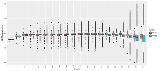
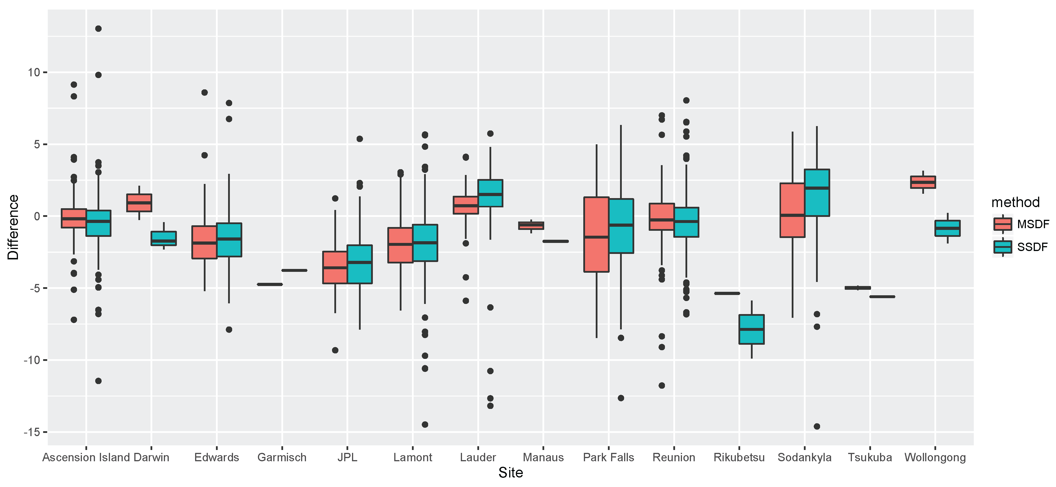
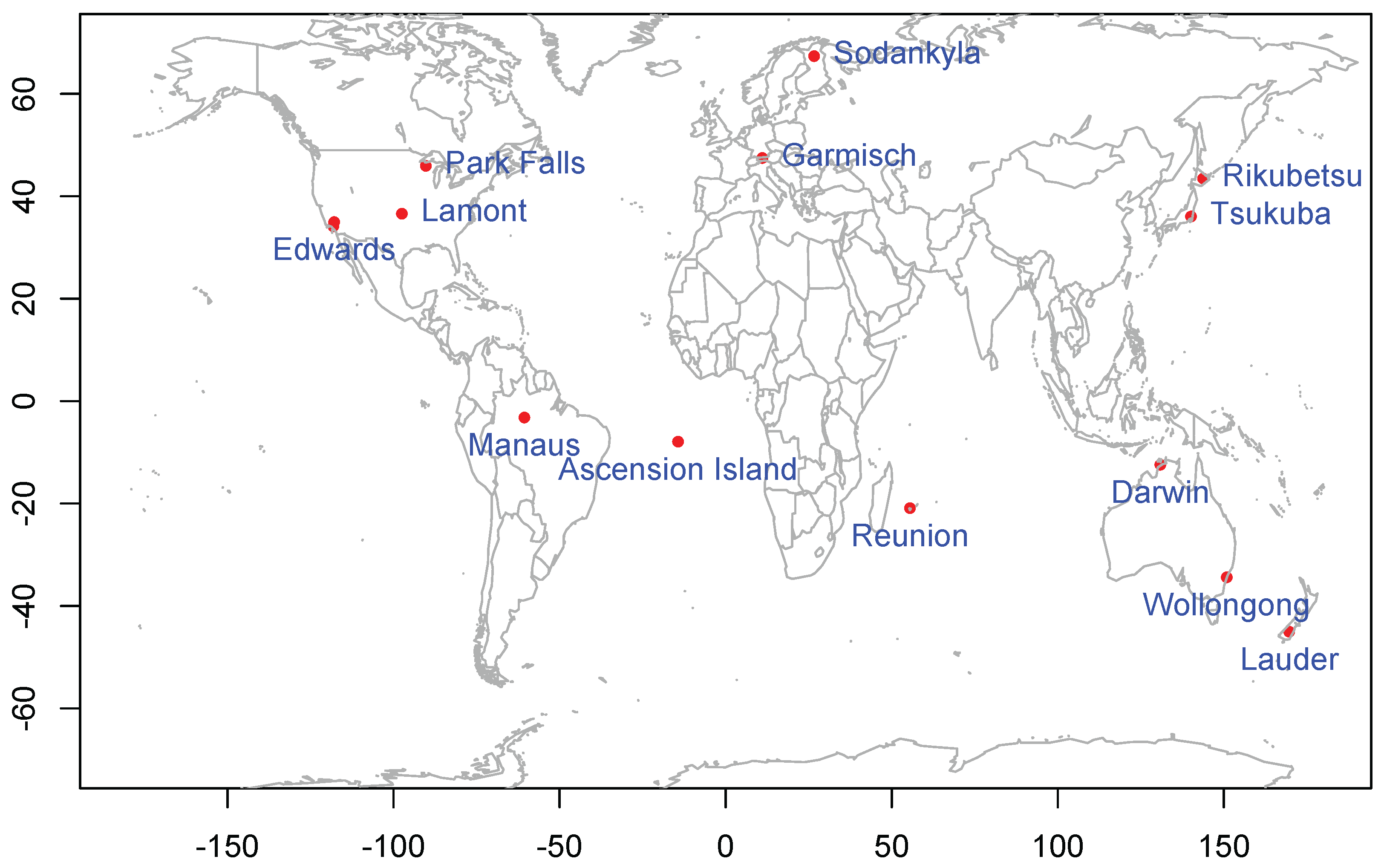
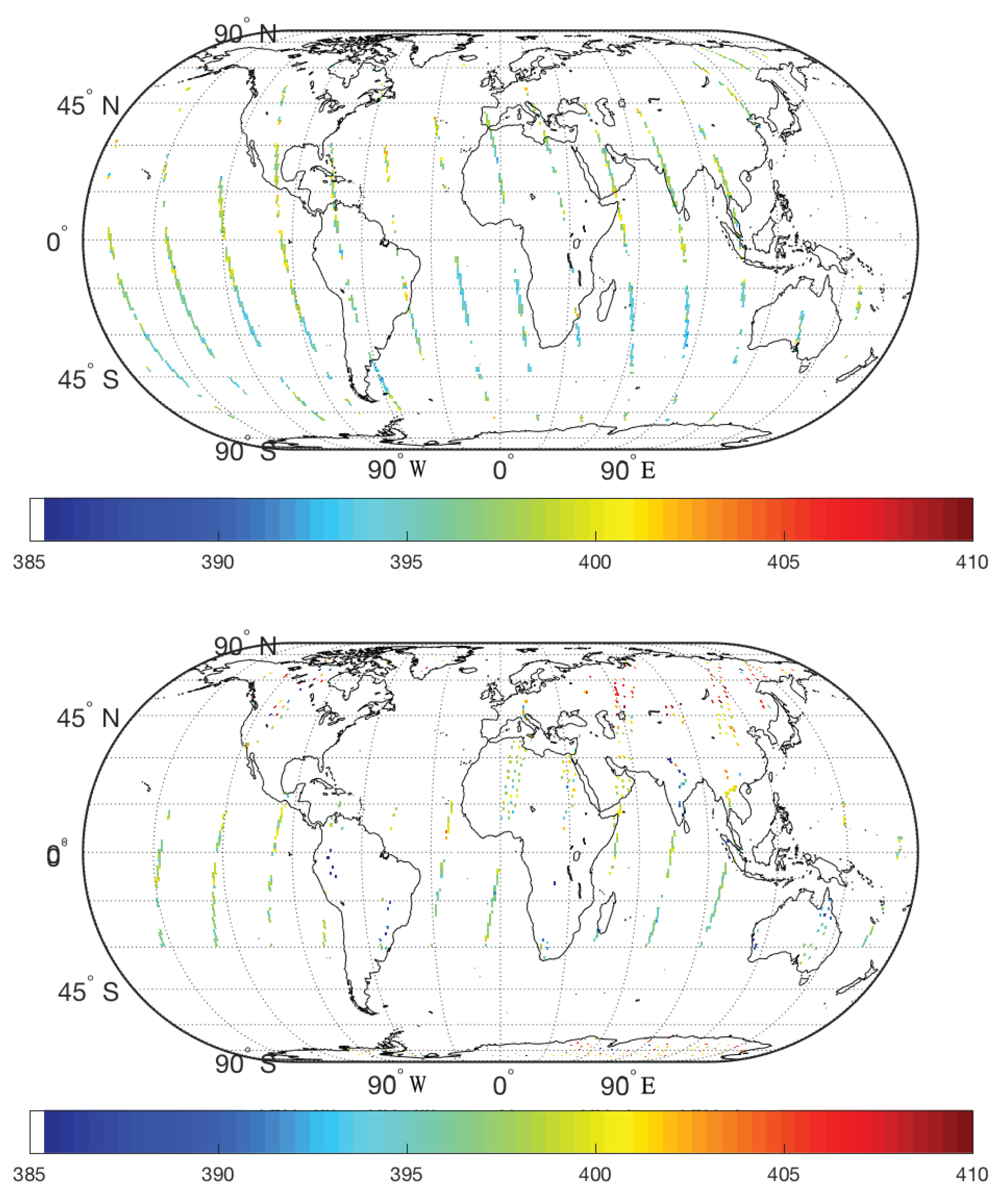
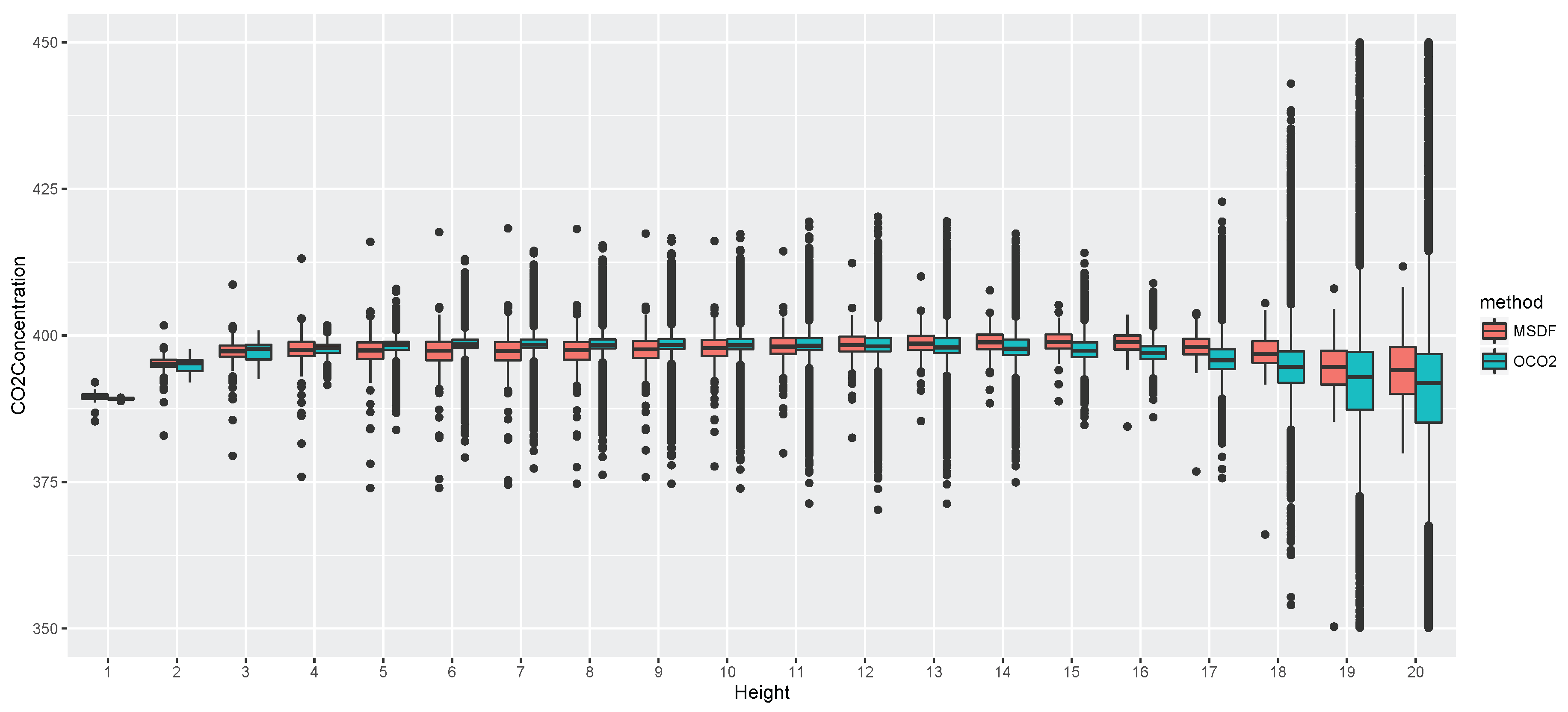
4. Application to CO2 Data from ACOS and OCO-2

In this section we present a demonstration of our MSDF methodology for fusing the ACOS (GOSAT) and OCO-2 profile data of CO2 and compare it to independent validation data. Unfortunately, ground-based CO2 profile data are mostly limited to aircraft flights or balloon campaigns, (e.g., [26]), which tend to be sparse in both spatial and temporal coverage. Because of this difficulty, we make use of column-averaged CO2 data from the Total Carbon Column Observing Network (TCCON) instead. These are a set of about 30 globally distributed ground-based stations that record daily observations of “total-column” (i.e., column-averaged) CO2. While this dataset does not provide a CO2 profile, we can convert our profile estimates at these TCCON locations into the corresponding column-averaged CO2 values for comparison. To assess the impact of accounting for the vertical dependence in the data-fusion algorithm, we also interpolate the already-column-averaged univariate CO2 data from ACOS and OCO-2 to the TCCON sites using two competing methods: (1) a simple coincidence criterion (SCC); and (2) a form of kriging modified to accommodate massive datasets (Spatial Statistical Data Fusion or SSDF; [4]). In what follows, we compare column-averaged MSDF, SCC, and SSDF estimates relative to the “ground-truth” TCCON values.

4.1. Overview of ACOS, OCO-2, and TCCON Data

The Greenhouse gases Observing Satellite (GOSAT) was launched on 23 January 2009 and the OCO-2 satellite was launched on 2 July 2014. As of August 2016, both instruments are still operational. For the period of comparison, we make use of OCO-2 and ACOS (i.e., GOSAT) Level 2 data between 1 January and 31 December 2015. We use the v3.5 release of the ACOS data, which are available from the Goddard Data and Information Services Center. Following recommendations from the ACOS Data User’s Guide, we apply the recommended data-screening procedure to eliminate potentially bad retrievals [27]. For the OCO-2 data, we use version 7.0, which is also available from the Goddard Data and Information Services Center . The OCO-2 data have a set of data-quality flags called Warn Levels [28], and for this exercise we only use data with Warn Levels less than 15. This particular filter eliminated about 25% of the converged OCO-2 data. For more information on both datasets, see [29,30].
The Total Carbon Column Observing Network (TCCON) consists of ground-based Fourier Transform Spectrometers that record direct solar spectra in the near-infrared. These spectra are then used to retrieve column-averaged abundances of atmospheric constituents including CO2, CH4, N2O, HF, CO, and H2O, which are directly comparable with the near-infrared column-averaged measurements from space-based instruments [31]. Whereas ACOS and OCO-2 retrievals are susceptible to variability resulting from contamination by optically thick clouds and aerosols that were missed by the cloud-screening process [10], TCCON makes direct observation of the solar disk and hence is less sensitive to errors from scattered light [32].
The TCCON sites sample in a diverse range of atmospheric states, which include tropical and polar, continental and maritime, polluted and clean, providing a valuable validation link between the high-coverage, medium-precision measurements from satellites (e.g., GOSAT and OCO-2) and a network of ground-based high-precision station measurements [31]. TCCON’s column-averaged CO2 data are in turn validated against integrated aircraft profiles [33,34,35,36] and have a precision and accuracy of ∼0.8 ppm [36]. We obtained TCCON data at all sites that were operational in 2015 via the TCCON Data Archive (see [37]). There were 27 of these sites, but only 14 produced data on days when both GOSAT and OCO-2 were operational in 2015. Their locations are presented in Figure 1. Fortunately, these 14 sites are fairly well distributed globally and include both continental and maritime regions as well as spanning a range of diverse geographical and ecological regimes.
For our demonstration, we obtained daily global ACOS and OCO-2 Level 2 data (using both the profile and column-averaged CO2 estimates) and fused them to produce MSDF and SSDF estimates of column-averaged CO2 at TCCON locations that have at least one ACOS or OCO-2 retrieval within 1000km on the same day. These two estimates are compared to each other and to a third estimate, the simple coincidence criterion (SCC) estimate, at each TCCON site. The SCC estimate is defined as the unweighted average of all ACOS and OCO-2 retrievals within 1000 km of said location, which could be considered as an “ad hoc” fusion. SCC and SSDF both operate on scalar column-averaged CO2 concentrations from ACOS and OCO-2, while MSDF operates on the 20-dimensional CO2 profiles for ACOS and OCO-2. The MSDF profile estimate is convolved into a column-averaged CO2 value using a linear combination pressure weighting function that is a function of the local specific humidity and the local acceleration due to gravity (see Appendix A of [10]). We did not account for temporal dependence in the observed data, treating all the data within the same day as if they were observed at a fixed time point.
These three estimates (SCC, SSDF, and MSDF) were then compared to the daily median CO2 values from the corresponding TCCON sites. Since both the scalar (SCC, SSDF) and profile (MSDF) fusions are spatial only, our research illustrates most clearly whether the extra effort involved in doing a multivariate data fusion is worth the effort.
Both the GOSAT and OCO-2 instruments have long periods of observation punctuated with brief periods of non-operation for reasons of maintenance, thermal control, or spacecraft maneuvers. For each day in 2015, we performed data fusion and estimated column-averaged CO2 at the TCCON sites if and only if both instruments produced observations on that day. There were 258 days in 2015 in which both instruments were operationally making observations. Typically, there are about 70,000 observations from OCO-2 per day, while GOSAT has about 2000 observations per day. Figure 2 illustrates the spatial patterns of each of the instruments on a particular day, 3 March 2015. Both maps show thin stripes of data running in a north-south direction, which are indicative of their polar, sun-synchronous orbits. Both instruments notably have sections of their observational swath missing, which is likely due to the retrieval process failing because of contamination from clouds. Note that OCO-2’s and GOSAT’s observational patterns are both reinforcing and complementary. In regions such as the southern oceans, their overlapping coverage can contribute to lower uncertainties in the estimates. In other places such as the high-latitude Siberian tundra, one instrument (in this case, GOSAT) is able to make observations while the other cannot. However, in the North American continent, the opposite is true.
The root mean squared error (RMSE) of column-averaged CO2 from OCO-2 is between 1.5–3.5 ppm over land and 1.5–2.5 ppm over ocean [38]. This figure includes the bias, which is typically between 1 and 2 ppm, and the variance. In a more recent study, Wunch, D. et al. [39] compared OCO-2 bias-corrected OCO-2 measurements against TCCON and found the RMSE to be typically under 1.5 ppm. For simplicity, we use a conservative constant value of 1.5 ppm for the measurement error’s standard deviation. There is no corresponding validation study for the ACOS v3.5 data due to its recent production, so we assume that its measurement-error standard deviation is also 1.5 ppm.
To the best of our knowledge, there has been no attempt in the literature to quantify the biases and measurement-error variance of the individual height-specific CO2 concentrations for either OCO-2 or ACOS. To obtain rough estimates of the height-specific measurement-error variance, { ( σ ϵ ( i , k ) ) 2 } , we first compute the empirical variance of the CO2-concentration data at each height. That is, we obtain an instrument-specific vector of empirical variances v ( i ) ( v ( i , 1 ) , , v ( i , K ) ) , where v ( i , k ) is the empirical variance of the elements in Z ( i , k ) . Similarly, we also compute a vector of the average pressure weighting function over the entire dataset, and we call it h ^ . We then average the retrieval covariance matrix across all retrieved values to produce the mean posterior covariance matrix Q ^ ( i ) . This matrix is then ‘normalized’ to produce Q ^ N as follows,
Q ^ N = I Q , i 1 / 2 Q ^ ( i ) I Q , i 1 / 2 ,
where I Q , i is a diagonal matrix with the same diagonal elements as Q ^ ( i ) . This produces a correlation matrix Q ^ N ( i ) with 1’s along the diagonal and inter-height correlations in the off-diagonal elements. We then specify that the measurement error { ( σ ϵ ( i , k ) ) 2 } is approximately equal to the diagonal of the matrix β ( i ) I v , i 1 / 2 Q ^ N ( i ) I v , i 1 / 2 , where I v , i is a diagonal matrix with v ( i ) along the diagonal, and β ( i ) is a constant for the i-th instrument and is chosen such that β ( i ) h ^ I v , i 1 / 2 Q ^ N ( i ) I v , i 1 / 2 h ^ = ( 1.5 ) 2 . For GOSAT and ACOS, we calculated this coefficient to be 0.36 and 0.33, respectively. Erring on the conservative side, we chose 0.40 as the coefficient for both instruments. Essentially, this procedure assigns about 40% of the marginal variability of CO2 at each height as the corresponding measurement-error variance.
Regarding the bias, the OCO-2 instrument team uses a linear bias correction scheme that estimates a bias in column-averaged CO2 at each location as a function of the footprint index, the difference between the retrieved and the a priori surface pressure; the relative abundance of coarse aerosols; and the variation in the retrieved profile from that assumed in the prior [28]. The coefficients of this bias-correction model are estimated by comparison to TCCON data and by using the so-called southern hemisphere approximation, which assumes that the entire region from 25 to 60 latitude has minimal and negligible variation in the signal for column-averaged CO2 [40]. ACOS v3.5 has a similar linear bias correction scheme for column-averaged CO2 [27]. These bias-correction schemes make it straightforward to remove the bias from the GOSAT and OCO-2 column-averaged CO2 values before fusing them with SSDF. However, at present it is not clear how to translate this linear bias-correction scheme in column-averaged CO2 into biases at each of the 20-dimensional CO2 concentrations, as is required for applying MSDF. Since we are principally concerned with understanding the effect of “vertical” CO2 dependence on inferences (i.e., MSDF versus SSDF), we opted not to apply bias correction on ACOS and OCO-2 data in our comparisons. We see later that we can detect this bias in the predictions, which is consistent for both MSDF and SSDF.
For the horizontal basis functions, we make use of multi-resolutional bisquare basis functions. Specifically, we use three resolutions whose centers are the centers of Level 1, 2, and 3, respectively, of an Icosahedral Snyder Equal Area Aperture 3 (ISEA3) grid, which is generated from the Discrete Global Grid software [24]. The three resolutions have 32, 92, and 272 basis centers, respectively, for a total of 396 functions. These basis centers are used for both MSDF and SSDF; and for the former a set of vertical basis functions based on cubic B-splines are also used, as discussed in Section 3.3. At each height, the EM algorithm’s initial values for the fine-scale and the small-scale parameters are set at 10% and 90%, respectively, of the difference between the empirical variance minus the measurement-error variance (see Supplementary Materials of [5] for more details).
Having performed the data fusions, we compare SCC, SSDF, and MSDF predictions to the TCCON daily median column-averaged CO2 values, of which there are 1055 separate values. Table 1 displays the Mean Squared Error (MSE), Mean, and Variance for the prediction errors. Looking at the MSE, we see that SSDF’s and MSDF’s are substantially smaller than SCC’s value of 7.84 ppm2, indicating that the principled framework underlying the statistical data fusions does capitalize on spatial dependence to improve the MSE. For a better understanding of the improvement, we also looked into the Mean and Variance in the bottom rows of Table 1. SCC has the worst Mean, also called bias, value of 1.49 ppm, while SSDF and MSDF have about the same average bias. This is not surprising, as we did not correct for the bias before carrying out data fusion. MSDF has a slightly larger bias than SSDF (1.36 ppm versus 1.31 ppm), but this is probably due to noise not signal.
While SSDF and MSDF do not differ very much with regard to the bias, they are different for the prediction-error variance. SSDF has a variance of 5.33 ppm2 (standard deviation = 2.31 ppm), while MSDF comes with a slightly improved variance of 5.03 ppm2 (standard deviation = 2.24 ppm), or about a 6% reduction in prediction-error variance. We note that MSDF’s MSE value of 6.87 ppm2 (RMSE = 2.62 ppm) is consistent with OCO-2 validation studies showing an RMSE of 1.5–3.5 ppm over land and 1.5–2.5 ppm over ocean [38]. Based on variance and MSE, the general ranking of the methods from best to worst is MSDF, followed by SSDF, followed by SCC.
The metrics in Table 1 are averaged across the 14 TCCON sites, and in Figure 3 we explore the improvement in detail through boxplots of the prediction errors at the individual sites. From this figure, the distribution of the errors within any particular TCCON site tends to have the same mean for both methods, which is consistent with the results of Table 1. One interesting feature from Figure 3 is that MSDF has fewer outliers overall than SSDF, indicated on the boxplots by dots extending far past the “whiskers.” This is especially noticable over Ascension Island, Lamont, Lauder, and Sodankyla. Overall, Figure 3 shows what statistical theory suggests. Data fusion of column-averaged CO2 based on MSDF does not improve upon the bias of an estimate, but it does reduce its variability.

5. Discussion

The results in Section 4 show that SSDF is able to improve upon SCC by accounting for horizontal spatial dependence. This is because SCC (defined as an average of all data points falling within a certain radius) is in essence a linear estimator of the form a s c c Z X C O 2 , where a s c c is a vector of averaging weights and Z X C O 2 is a vector of all the observed total-column CO2. SSDF is also a linear estimator of the form a s s d f Z X C O 2 , but here the weights are computed such that the expected squared error relative to the truth is minimized (for more detail, see [4]). Since SCC is a linear estimator, its prediction error should always be larger than or equal to that of the best linear unbiased estimator SSDF. Similarly, we can view SSDF as a restricted linear estimator on the much larger space of the profile data. To see this, let x ( s ) be the 20-dimensional CO2 profile at location s , and let Z * = ( x ( s 1 ) , x ( s 2 ) , , x ( s N ) ) be the ( 20 N ) -dimensional vector of stacked profiles. Without loss of generality, assume that we are considering a dataset from one instrument with no bias. The total column CO2 value, χ ( s ) , is given by
χ ( s ) = h ( s ) x ( s ) ,
where h ( s ) = ( h 1 ( s ) , , h 20 ( s ) ) is the pressure weighting vector of coefficients of the profile values, x ( s ) .
In both SSDF and MSDF, we try to compute the vector of kriging coefficients that minimizes the expected squared error at a prediction location s 0 . For MSDF, this involves computing the estimates
χ ^ m ( s 0 ) = h ( s 0 ) a 1 a 2 a 20 Z * ,
with the unbiasedness constraint 1 a k = 1 , where a k = ( a k , 1 , a k , 2 , , a k , 20 N ) is ( 20 N ) -dimensional. For SSDF, this involves minimizing the prediction error for the following estimate:
χ ^ s ( s 0 ) = a * Z X C O 2 = a * h ( s 1 ) 0 0 h ( s 2 ) h ( s N ) x ( s 1 ) x ( s 2 ) x ( s N ) = a * h ( s 1 ) 0 0 h ( s 2 ) h ( s N ) Z * ,
subject to the constraint 1 a * = 1 where a * = ( a * , 1 , a * , 2 , , a * , N ) is N-dimensional.
Comparing (22) and (23), we see that MSDF has a prediction advantage because it incorporates the true pressure weighting function at the prediction location s 0 in its computation, taking advantage of the definition in (21). SSDF, on the other hand, has to ‘interpolate’ the effect of that pressure weighting function from nearby observations. Even if we remove the advantage from the knowledge of h ( s 0 ) , MSDF still has better theoretical performance. We can see this by setting the pressure weighting function to be constant. That is, we assume that h ( s ) = h = ( h 1 , , h 20 ) . Plugging h into (22) and (23) and multiplying the first two terms on the right hand side results in the following simplifications:
χ ^ m ( s 0 ) = a m Z * , χ ^ s ( s 0 ) = a s Z * ,
where a m and a s are both ( 20 N ) -dimensional with the following forms:
a m = k = 1 20 h k a k , 1 k = 1 20 h k a k , 2 k = 1 20 h k a k , 20 N , and   a s = h λ ( 1 ) a * , γ ( 1 ) h λ ( 2 ) a * , γ ( 2 ) h λ ( 20 N ) a * , γ ( 20 N ) .
where λ ( l ) = 1 + ( ( l 1 ) mod 20 ) and γ ( l ) = l / 20 , where x indicates the smallest integer greater than or equal to x.
Examining (24), we see that both SSDF and MSDF can be seen as linear combinations of the elements in the ( 20 N ) -dimensional vector Z * . However, SSDF is minimizing the error over the space spanned by the N-dimensional a * , which does not account for interaction effects among the 20 profile levels, while MSDF is minimizing the expected error over a much larger space spanned by { a i : i = 1 , , 20 } . On average, MSDF should return smaller error than SSDF. Another way to interpret this is that SSDF is accounting for horizontal spatial dependence, and MSDF improves upon SSDF through the further incorporation of vertical dependence.
Yet another way to understand the improvement in prediction-error variance is by comparing the scalar estimates to the MSDF prediction, with regard to the latter’s ability to dampen more efficiently the large variability of the retrieved CO2 at specific heights. Retrieving CO2 concentrations at 20 different heights from photon counts is a difficult process and, in particular, the OCO-2 retrieval algorithm that yields the profile vector of CO2 concentrations has large variability in the estimates of individual components. While the empirical measurement-error standard deviation of the column-averaged CO2, compared to validation data, is about 2–3 ppm, the standard deviations of the individual components, particularly those at lower heights, can be much larger. We demonstrated this by collecting all retrieved profiles from OCO-2 within 100 km of the Darwin, Australia TCCON site and compared them to the fused estimates from MSDF at the same location. In Figure 4, we give the boxplots of CO2 concentration as a function of height for both the OCO-2 values and the MSDF predicted values. Recall that the total-column CO2 values are obtained by applying a pressure weighting function to the 20-dimensional profiles. The OCO-2 retrieved profiles and the MSDF profiles have the same mean within each pressure level, so we can expect that the total-column CO2 produced from these two datasets would have the same means. However, statistical theory suggests that MSDF estimates will have much smaller variability compared to the OCO-2 profile data, and hence, in principle its total-column CO2 should have smaller variance. This is supported by the results in Table 1, indicating that our methodology is able to take advantage of the vertical dependence in addition to the horizontal dependence to dampen the inherently large “measurement error” in the retrieved profile vectors.
Another practical implication of Figure 4 is that the smoothed estimates, with their much-reduced variability, are more conducive to studies of CO2 trends and evolution at specific heights. In this article we have motivated MSDF in terms of deriving a better total column CO2, and we have demonstrated this by optimally estimating the entire profile at once and then applying a linear combination to the profile to retrieve the total column CO2. In principle, however, the CO2 concentrations from MSDF are potentially useful in and of themselves. Typically, CO2 concentrations at individual heights are overlooked in carbon-cycle analysis due to their large variability and the low degrees of freedom in the vertical direction. Hence, scientific analyses predominantly focus on total column CO2, even though in many applications it is the height-specific behaviors that are of primary interest. For instance, the exchange of CO2 between the atmosphere and Earth’s surface is a critical part of the global carbon cycle and an important determinant of future climate [41]. Of particular interest to climate scientists is the global distribution of CO2 flux, or the net amount of CO2 exchanged between the atmosphere and the terrestrial biomes (plants, oceans, etc.) per unit of time. This could be approximated by selecting the CO2 concentrations corresponding to the surface from the MSDF CO2 profiles, and then differencing with respect to time. Statistical theory suggests that this idea should work, but its feasibility and robustness will need to be explored in further research.

6. Conclusions

This article examines a methodology for estimating column-averaged CO2 from two remote sensing instruments—GOSAT and OCO-2. Both instruments produce multivariate profile CO2 values and a column-averaged CO2 value that is a linear combination of the profile with coefficients given by a deterministic pressure weighting function. Derivative uses of the CO2 data such as Level 3 map generation or colocation for instrument validation tend to make use of the column-averaged CO2 field. We show here that there is information in the profile that is potentially lost when the individual profiles are first convolved with the pressure weighting function. In the Application section, we show that performing multivariate data fusion on the profile first, and then convolving the fused profile prediction into the univariate column-averaged CO2 value afterwards, has smaller mean squared error. We note that this result is in line with the conventional wisdom that OCO-2 has between 1 and 2 degrees of freedom along the vertical column. The process of convolving the column vector into a total-column scalar value is a lossy process, and the improvement we observed in the Application section is due to our multivariate methodology being better able to capitalize on the extra degrees of freedom along the column in the spatial interpolation process.
The datasets in this application are fairly large, totaling about 70,000 observations per day. This is not a problem for MSDF, which has computational complexity that is linear with respect to the data size. Furthermore, MSDF does not assume isotropy or stationarity in the data, which makes it appropriate for a wide range of applications. Note that having large amounts of data yields robust estimates of the spatial-dependence parameters through the EM algorithm. Hence, the methodology is well suited for data-rich applications, where the dependence on massive amounts of data is a strength rather than a weakness. This is particularly relevant to remote sensing, where a typical instrument returns thousands to hundreds of thousand of observations per day, and future instruments will be able to return millions of observations per day.
One direction for further research is incorporating temporal dependence into the model. We could allow the parameter η to evolve in discrete time steps according to a first-order autoregressive process as demonstrated in [5,20]. In principle, that approach can be applied to the MSDF algorithm, but we anticipate that the main challenge would be the need to estimate the significantly larger propagation and innovation matrices. Further research is needed to balance the computational needs of a spatio-temporal MSDF against robustness of the data fusion.

Acknowledgments

We would like to thank the reviewers and the editor of Remote Sensing for their insightful comments. The research described in this paper was carried out in part by the Jet Propulsion Laboratory, California Institute of Technology, under a contract with NASA. It is supported by NASA’s Earth Science Technology Office through its Advanced Information Systems Technology program. Noel Cressie’s research was also partially supported by a 2015–2017 Discovery Grant, DP150104576, from the Australian Research Council, and by NASA grant NNHII-ZDA001N-OCO2. ACOS and OCO-2 data were obtained from Goddard Earth Sciences Data and Information Services Center, operated by NASA, from the website http://daac.gsfc.nasa.gov/. TCCON data were obtained from the TCCON Data Archive, hosted by the Carbon Dioxide Information Analysis Center, from the website http://tccon.ornl.gov/.

Author Contributions

All authors contributed to the design of the methodology and the validation exercise; H. Nguyen and N. Cressie wrote the paper.

Conflicts of Interest

The authors declare no conflict of interest.

References

  1. Houghton, J.T.; Ding, Y.; Griggs, D.J.; Noguer, M.; van der Linden, P.J.; Dai, X.; Maskell, K.; Johnson, C.A. Climate Change 2001: The Scientific Basis; Contribution of Working Group I to the Third Assessment Report of the Intergovernmental Panel on Climate Change; Cambridge University Press: Cambridge, UK, 2001. [Google Scholar]
  2. Rodgers, C.D. Inverse Methods for Atmospheric Sounding: Theory and Practice; World Scientific: River Edge, NJ, USA, 2000. [Google Scholar]
  3. Crisp, D.; Boesch, H.; Brown, L.; Castano, R.; Christi, M.; Conner, B.; Frankenberg, C.; McDuffie, J.; Miller, C.; Natraj, V.; et al. OCO (Orbiting Carbon Observatory): Level 2 Full Physics Retrieval Algorithm Theoretical Basis; Jet Propulsion Laboratory, NASA: Pasadena, CA, USA, 2010. [Google Scholar]
  4. Nguyen, H.; Cressie, N.; Braverman, A. Spatial statistical data fusion for remote sensing applications. J. Am. Stat. Assoc. 2012, 107, 1004–1018. [Google Scholar] [CrossRef]
  5. Nguyen, H.; Katzfuss, M.; Cressie, N.; Braverman, A. Spatio-Temporal Data Fusion for Very Large Remote Sensing Datasets. Technometrics 2014, 56, 174–185. [Google Scholar] [CrossRef]
  6. Kulawik, S.S.; O’Dell, C.; Payne, V.H.; Kuai, L.; Worden, H.M.; Biraud, S.C.; Sweeney, C.; Stephens, B.; Iraci, L.T.; Yates, E.L.; Tanaka, T. Lower-tropospheric CO2 from near-infrared ACOS-GOSAT observations. Atmos. Chem. Phys. Discuss. 2016, 2016, 1–55. [Google Scholar] [CrossRef]
  7. Cressie, N.; Johannesson, G. Fixed rank kriging for very large spatial data sets. J. R. Stat. Soc. Ser. B 2008, 70, 209–226. [Google Scholar] [CrossRef]
  8. Hamazaki, T.; Kaneko, Y.; Kuze, A.; Kondo, K. Fourier transform spectrometer for Greenhouse Gases Observing Satellite (GOSAT). In Proceedings of the International Society for Optical Engineering (SPIE) Symposium, Remote Sensing of the Atmosphere, Ocean, Environment, and Space, Honoluu, HI, USA, 8–12 November 2004.
  9. Morino, I.; Uchino, O.; Inoue, M.; Yoshida, Y.; Yokota, T.; Wennberg, P.O.; Toon, G.C.; Wunch, D.; Roehl, C.M.; Notholt, J.; et al. Preliminary validation of column-averaged volume mixing ratios of carbon dioxide and methane retrieved from GOSAT short-wavelength infrared spectra. Atmos. Meas. Tech. 2011, 4, 1061–1076. [Google Scholar] [CrossRef]
  10. O’Dell, C.W.; Connor, B.; Bösch, H.; O’Brien, D.; Frankenberg, C.; Castano, R.; Christi, M.; Eldering, D.; Fisher, B.; Gunson, M.; et al. The ACOS CO2 retrieval algorithm Part 1: Description and validation against synthetic observations. Atmos. Meas. Tech. 2012, 5, 99–121. [Google Scholar] [CrossRef]
  11. Cressie, N. Change of support and the modifiable areal unit problem. Geogr. Syst. 1996, 3, 159–180. [Google Scholar]
  12. Berliner, L.; Wikle, C.; Milliff, R. Multiresolution Wavelet Analyses in Hierarchical Bayesian Turbulence Models. In Bayesian Inference in Wavelet-Based Models; Miller, P., Vidakovic, B., Eds.; Springer Lecture Notes in Statistics, No. 141; Springer: New York, NY, USA, 1999. [Google Scholar]
  13. Wikle, C.K.; Milliff, R.F.; Nychka, D.; Berliner, L.M. Spatio-Temporal hierarchical Bayesian modeling: Tropical ocean surface winds. J. Am. Stat. Assoc. 2001, 96, 382–397. [Google Scholar] [CrossRef]
  14. Nychka, D.; Wikle, C.K.; Royle, J. Multiresolution models for nonstationary spatial covariance functions. Stat. Model. 2002, 2, 315–331. [Google Scholar] [CrossRef]
  15. Hooten, M.B.; Larsen, D.R.; Wikle, C.K. Predicting the spatial distribution of ground flora on large domains using a hierarchical Bayesian model. Landsc. Ecol. 2003, 18, 487–502. [Google Scholar] [CrossRef]
  16. Royle, J.; Wikle, C. Efficient Statistical Mapping of Avian Count Data. Ecol. Environ. Stat. 2005, 12, 225–243. [Google Scholar] [CrossRef]
  17. Banerjee, S.; Gelfand, A.E.; Finley, A.O.; Sang, H. Gaussian prediction process models for large spatial data sets. J. R. Stat. Soc. Ser. B 2008, 70, 825–848. [Google Scholar] [CrossRef] [PubMed]
  18. Calder, C. A Bayesian dynamic process convolution approach to modelling the point distribution of PM2.5 and PM10. Envirometrics 2008, 19, 39–48. [Google Scholar] [CrossRef]
  19. Stein, M.L.; Jun, M. Nonstationary covariance models for global data. Ann. Appl. Stat. 2008, 2, 1271–1289. [Google Scholar]
  20. Cressie, N.; Shi, T.; Kang, E.L. Fixed Rank Filtering for Spatio-Temporal Data. J. Comput. Graph. Stat. 2010, 19, 724–745. [Google Scholar] [CrossRef]
  21. Lindgren, F.; Rue, H.; Lindstrom, J. An explicit link between Guassian fields and Gaussian Markov random fields: The stochastic partial different equation approach. J. R. Stat. Soc. Ser. B 2011, 73, 423–498. [Google Scholar] [CrossRef]
  22. Henderson, H.; Searle, S. On deriving the inverse of a sum of matrices. SIAM Rev. 1981, 23, 53–60. [Google Scholar] [CrossRef]
  23. Katzfuss, M.; Cressie, N. Spatio-temporal smoothing and EM estimation for massive remote-sensing data sets. J. Time Ser. Anal. 2011, 32, 430–446. [Google Scholar] [CrossRef]
  24. Carr, D.; Kahn, R.; Sahr, K.; Olsen, T. ISEA discrete global grids. Stat. Comput. Stat. Graph. 1998, 8, 31–39. [Google Scholar]
  25. Bartels, R.H.; Beatty, J.C.; Barsky, B.A. Hermite and Cubic Spline Interpolation; Morgan Kaufmann: San Francisco, CA, USA, 1998. [Google Scholar]
  26. Karion, A.; Sweeney, C.; Tans, P.; Newberger, T. AirCore: An Innovative Atmospheric Sampling System. J. Atmos. Ocean. Technol. 2010, 27. [Google Scholar] [CrossRef]
  27. Osterman, G.; Eldering, A.; Avis, C.; O’Dell, C.; Martinez, E.; Crisp, D.; Frankenberg, C.; Fisher, B. ACOS Level 2 Standard Product Data User’s Guide v3.5. Revision Date: Revision D, 6 March 2016. Available online: http://disc.sci.gsfc.nasa.gov/OCO-2/documentation/gosat-acos/gosat-acosdoc/ACOS_v3.5_DataUsersGuide.pdf (accessed on 15 May 2016).
  28. Osterman, G.; Eldering, A.; Avis, C.; Chafin, B.; O’Dell, C.; Frankenberg, C.; Fisher, B.; Mandrake, L.; Wunch, D.; Granat, R.; et al. OCO2 Data Product User’s Guide, Operational L1 and L2 Data Versions 7 and 7R. Revision Date: Version G, 30 June 2016. Available online: http://disc.sci.gsfc.nasa.gov/OCO-2/documentation/oco-2-v7/OCO2_DUG.V7.pdf (accessed on 23 May 2016).
  29. ACOS Data Access. Goddard Earth Sciences Data and Information Services Center. Available online: http://disc.sci.gsfc.nasa.gov/acdisc/documentation/ACOS.shtml (accessed on 23 May 2016).
  30. OCO-2 Data Access. Goddard Earth Sciences Data and Information Services Center. Available online: http://disc.sci.gsfc.nasa.gov/OCO-2 (accessed on 23 May 2016).
  31. Wunch, D.; Toon, G.; Blavier, J.; Washenfelder, R.; Notholt, J.; Connor, B.; Griffith, D.; Sherlock, V.; Wennberg, P. The Total Carbon Column Observing Network. Philos. Trans. R. Soc. A 2011, 369, 2087–2112. [Google Scholar] [CrossRef] [PubMed]
  32. Crisp, D.; Fisher, B.M.; O’Dell, C.; Frankenberg, C.; Basilio, R.; Boesch, H.; Brown, L.R.; Castano, R.; Connor, B.; Deutscher, N.M.; et al. The ACOS CO2 retrieval algorithm—Part II: Global XCO2 data characterization. Atmos. Meas. Tech. 2012, 5, 687–707. [Google Scholar] [CrossRef]
  33. Washenfelder, R.A.; Toon, G.C.; Blavier, J.F.; Yang, Z.; Allen, N.T.; Wennberg, P.O.; Vay, S.A.; Matross, D.M.; Daube, B.C. Carbon dioxide column abundances at the Wisconsin Tall Tower site. J. Geophys. Res. Atmos. 2006, 111, D22305. [Google Scholar] [CrossRef]
  34. Deutscher, N.M.; Griffith, D.W.T.; Bryant, G.W.; Wennberg, P.O.; Toon, G.C.; Washenfelder, R.A.; Keppel-Aleks, G.; Wunch, D.; Yavin, Y.; Allen, N.T.; et al. Total column CO2 measurements at Darwin, Australia-site description and calibration against in situ aircraft profiles. Atmos. Meas. Tech. 2010, 3, 947–958. [Google Scholar] [CrossRef]
  35. Messerschmidt, J.; Geibel, M.C.; Blumenstock, T.; Chen, H.; Deutscher, N.M.; Engel, A.; Feist, D.G.; Gerbig, C.; Gisi, M.; Hase, F.; et al. Calibration of TCCON column-averaged CO2: The first aircraft campaign over European TCCON sites. Atmos. Chem. Phys. 2011, 11, 10765–10777. [Google Scholar] [CrossRef]
  36. Wunch, D.; Toon, G.C.; Wennberg, P.O.; Wofsy, S.C.; Stephens, B.B.; Fischer, M.L.; Uchino, O.; Abshire, J.B.; Bernath, P.; Biraud, S.C.; et al. Calibration of the Total Carbon Column Observing Network using aircraft profile data. Atmos. Meas. Tech. 2010, 3, 1351–1362. [Google Scholar] [CrossRef] [Green Version]
  37. TCCON Data Access. TCCON Data Archive. Available online: http://tccon.ornl.gov/ (accessed on 23 May 2016).
  38. Connor, B.; Boesch, H.; McDuffie, J.; Taylor, T.; Fu, D.; Frankenberg, C.; O’Dell, C.; Payne, V.; Gunson, M.; Pollock, R.; et al. Quantification of Uncertainties in OCO-2 Measurements of XCO2: Simulations and Linear Error Analysis. Atmos. Meas. Tech. Discuss. 2016, 9, 5227–5238. [Google Scholar] [CrossRef]
  39. Wunch, D.; Wennberg, P.O.; Osterman, G.; Fisher, B.; Naylor, B.; Roehl, C.M.; O’Dell, C.; Mandrake, L.; Viatte, C.; Griffith, D.W.; et al. Comparisons of the Orbiting Carbon Observatory-2 (OCO-2) XCO2 measurements with TCCON. Atmos. Meas. Tech. Discuss. 2016, 2016. [Google Scholar] [CrossRef]
  40. Wunch, D.; Wennberg, P.O.; Toon, G.C.; Connor, B.J.; Fisher, B.; Osterman, G.B.; Frankenberg, C.; Mandrake, L.; O’Dell, C.; Ahonen, P.; et al. A method for evaluating bias in global measurements of CO2 total columns from space. Atmos. Chem. Phys. 2011, 11, 12317–12337. [Google Scholar] [CrossRef]
  41. Gruber, N.; Gloor, M.; Fletcher, S.E.M.; Dutkiewicz, S.; Follows, M.; Doney, S.C.; Gerber, M.; Jacobson, A.R.; Lindsay, K.; Menemenlis, D.; et al. Oceanic sources, sinks, and transport of atmospheric CO2. Glob. Biochem. Cycles 2009, 23. [Google Scholar] [CrossRef]
Figure 1. Locations of the 14 TCCON sites that were used to compare to column-averaged, data-fused CO2 values.
Remotesensing 09 00142 g001
Figure 2. Retrieved column-averaged CO2 data from OCO-2 (top panel) and ACOS (GOSAT) (bottom panel) on 3 March 2015.
Remotesensing 09 00142 g002
Figure 3. Boxplots of the “predicted minus TCCON” column-averaged CO2, where “predicted” is given by SSDF (teal) and MSDF (red).
Remotesensing 09 00142 g003
Figure 4. Boxplots of CO2 concentrations for MSDF predictions and colocated OCO-2 retrieved profiles at Darwin. Heights on the horizontal axis are the index k from height h k ; k = 1 , , 20 .
Remotesensing 09 00142 g004
Table 1. Table of MSE, Mean (Bias), and Variance of prediction errors.
SCCSSDFMSDF
MSE7.84167.04986.8741
Mean1.49361.30981.3582
Variance5.61085.33425.0294

