
Mapping Seasonal Inundation Frequency (1985–2016) along the St-John River, New Brunswick, Canada using the Landsat Archive

Abstract
:
1. Introduction
2. Materials and Methods
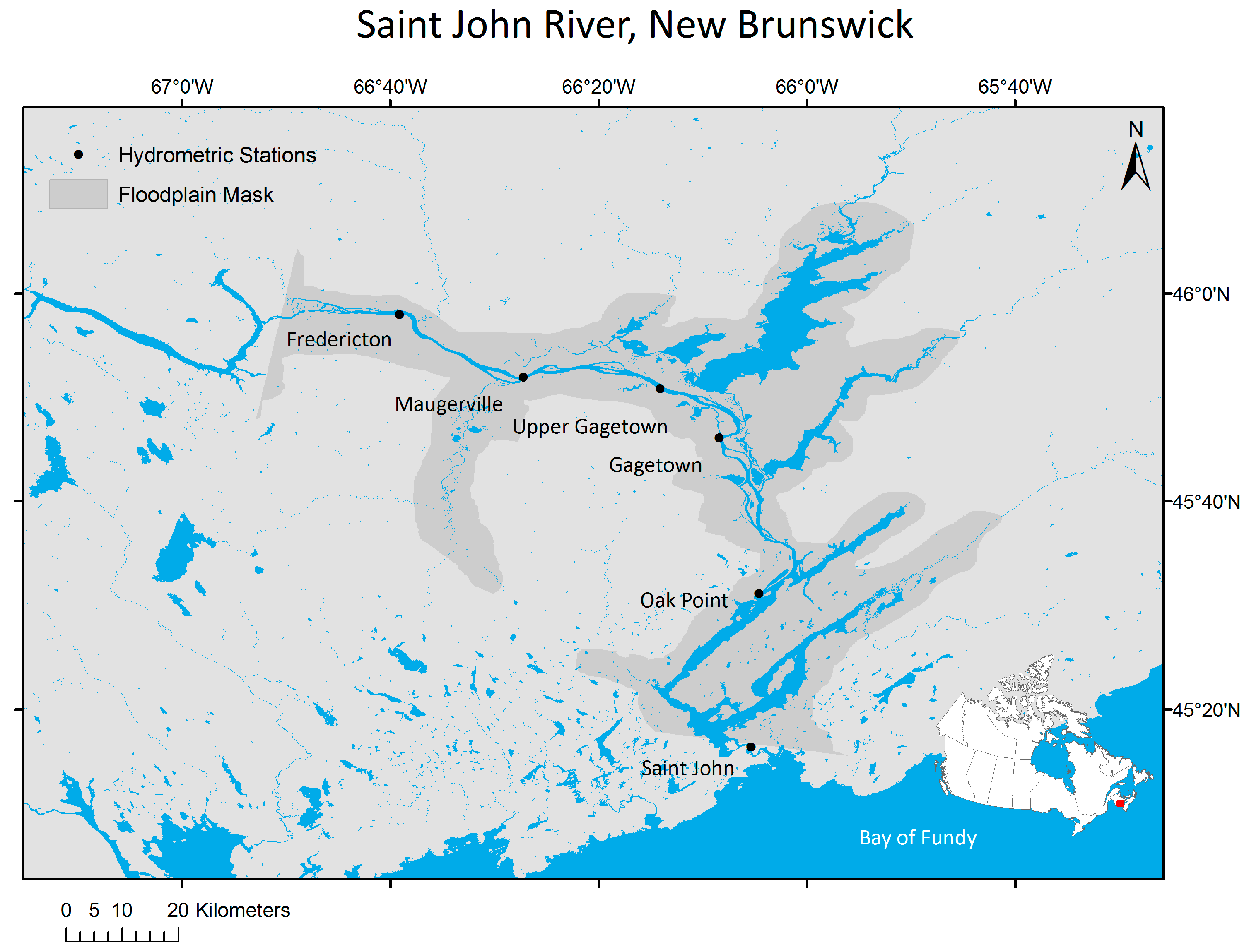
2.1. Study Area
2.2. Data
2.2.1. Landsat
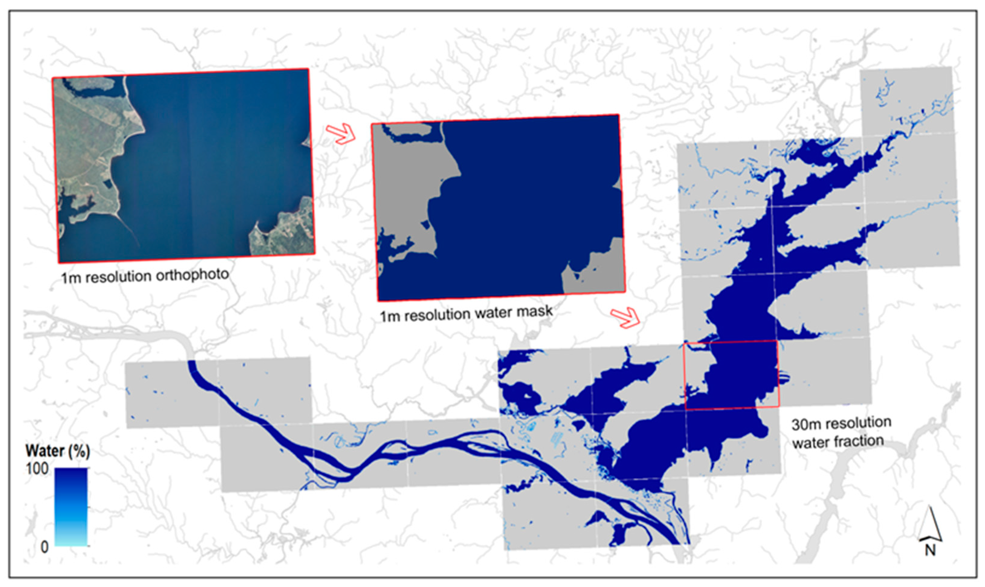
2.2.2. Orthophotos
2.2.3. Hydrometric Data
2.2.4. CanVec Data
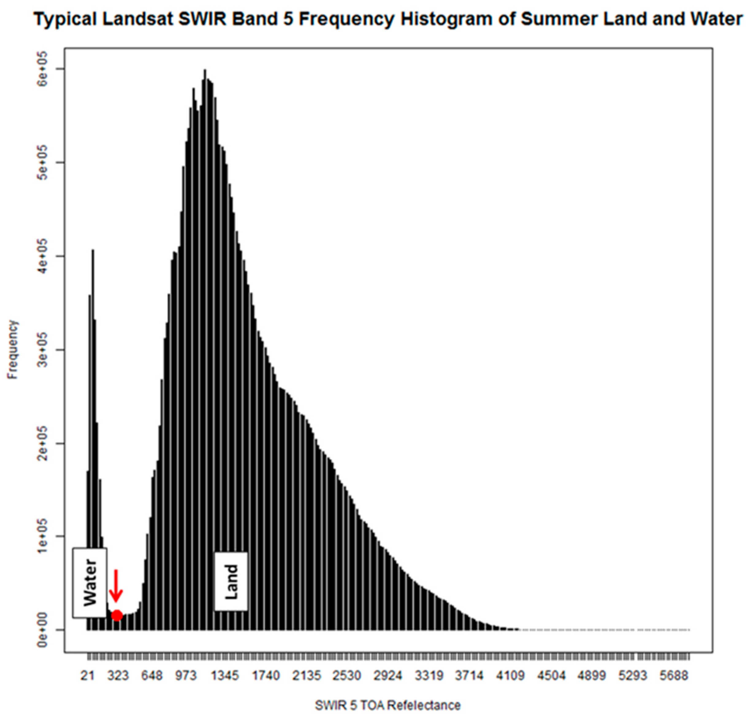
2.3. Water Classification
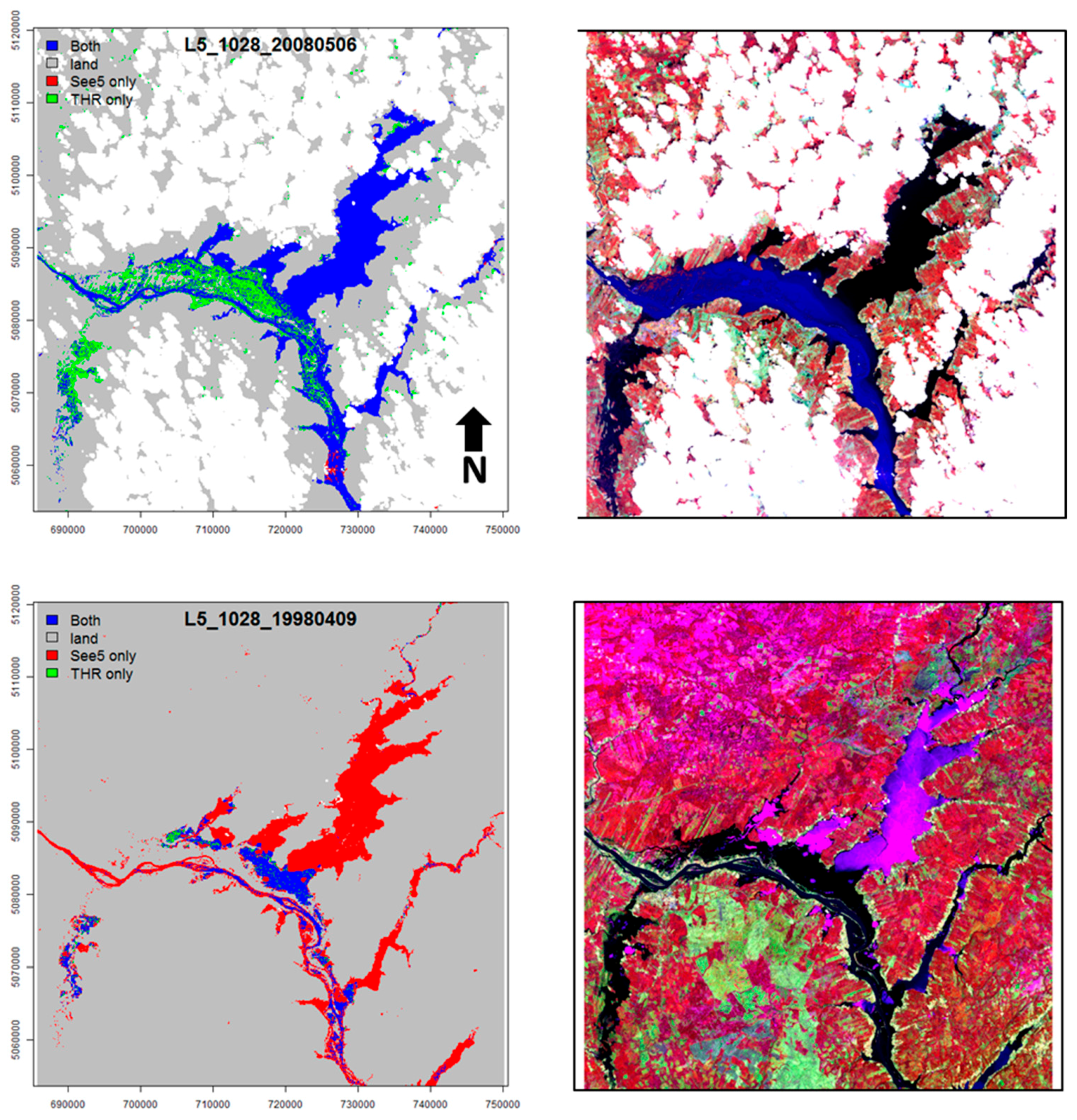
2.4. Validation
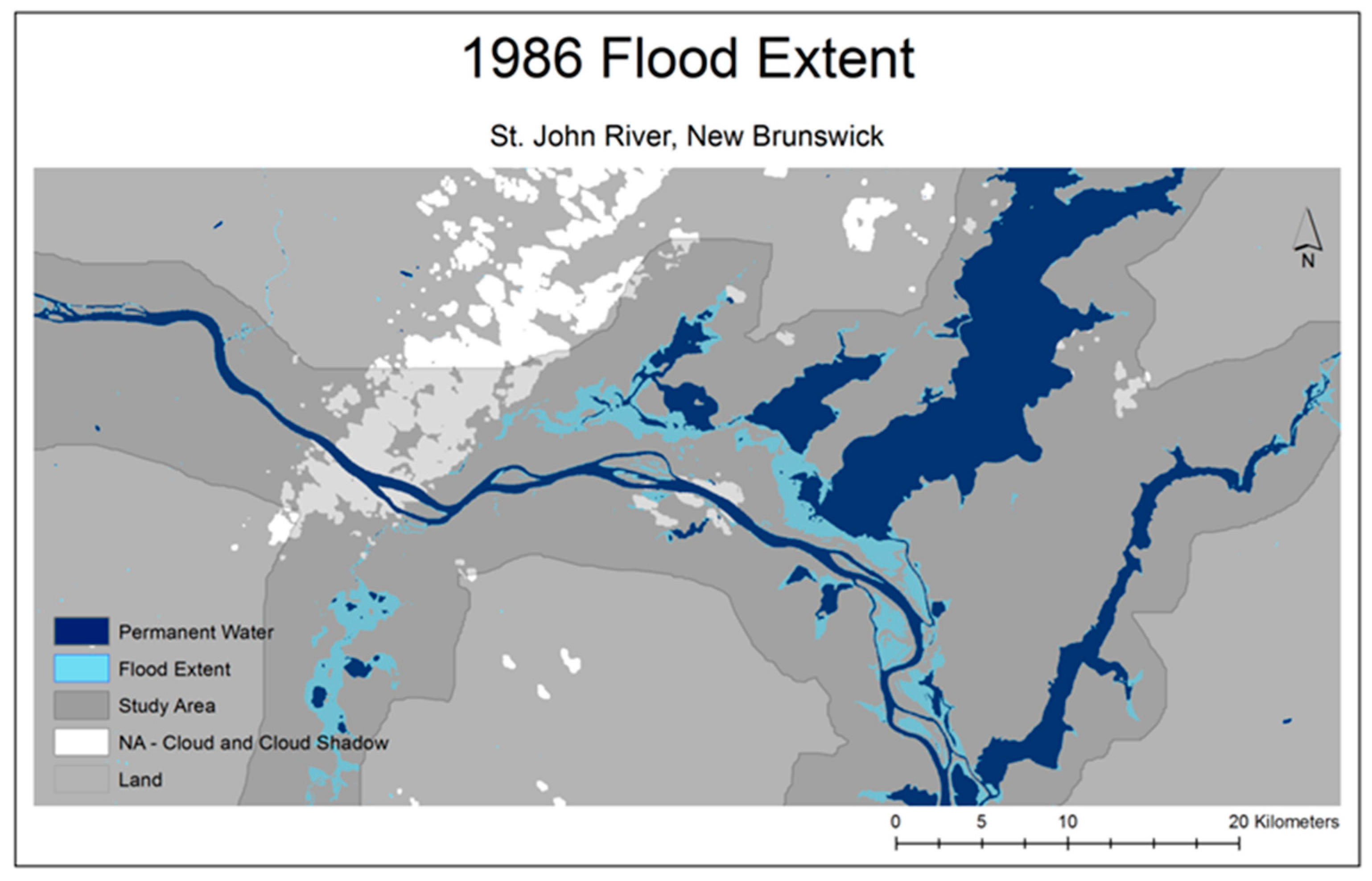
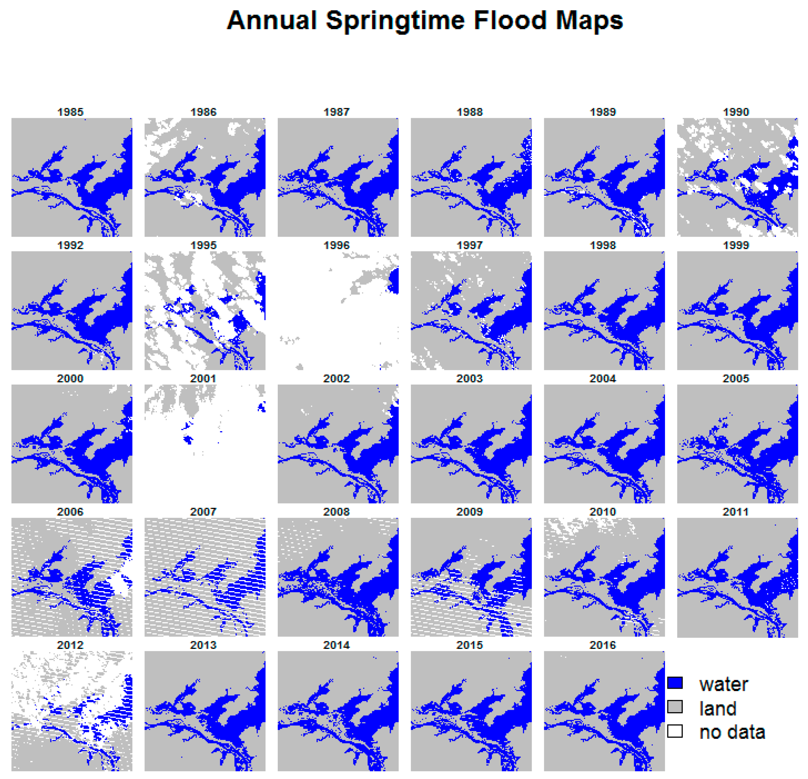
3. Results
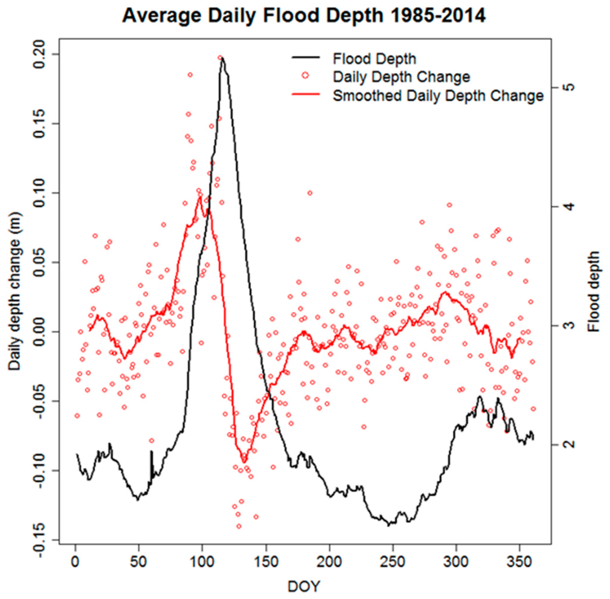
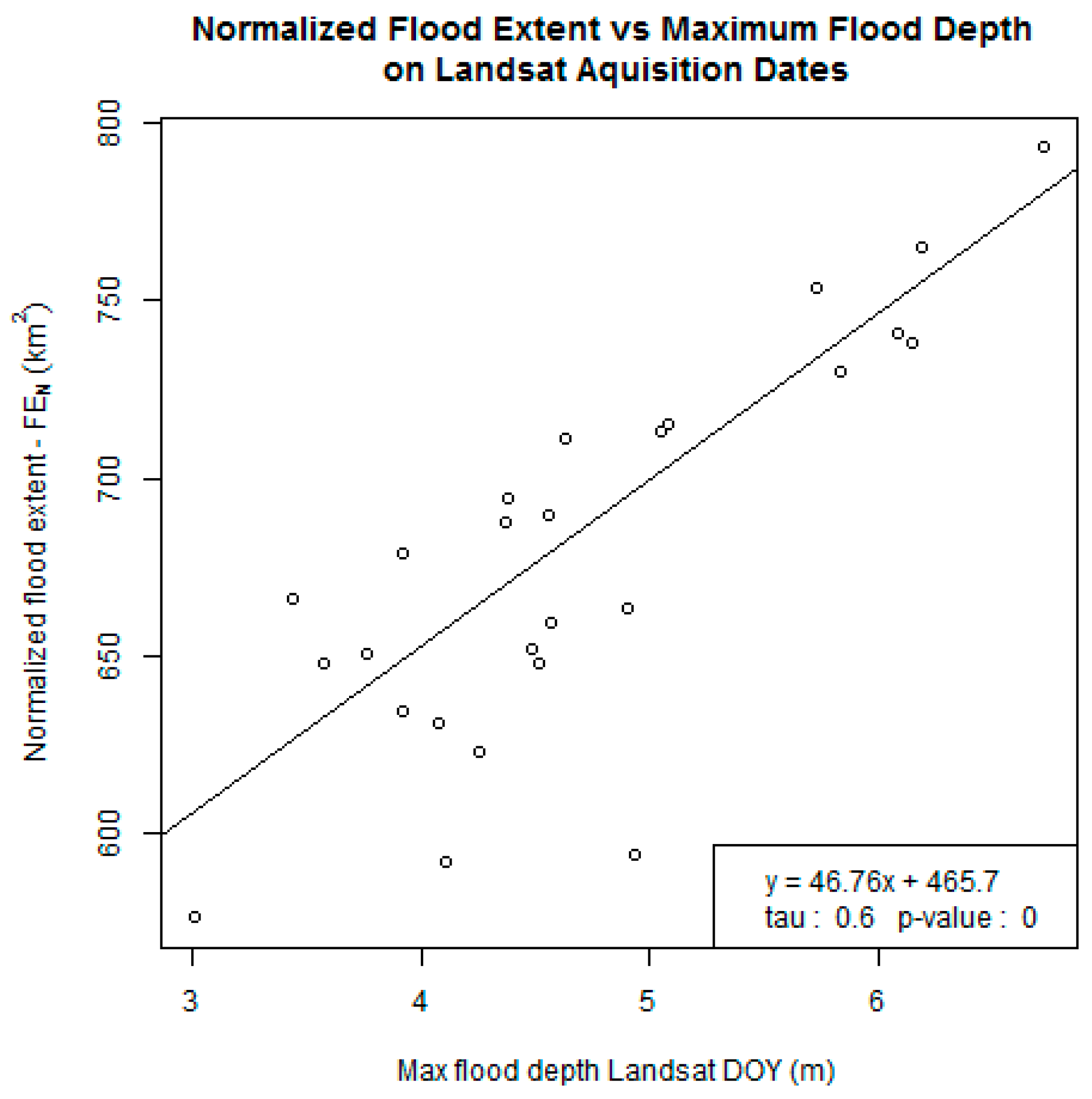
3.1. Assessment—Spring Water Extents vs. Flood Depth
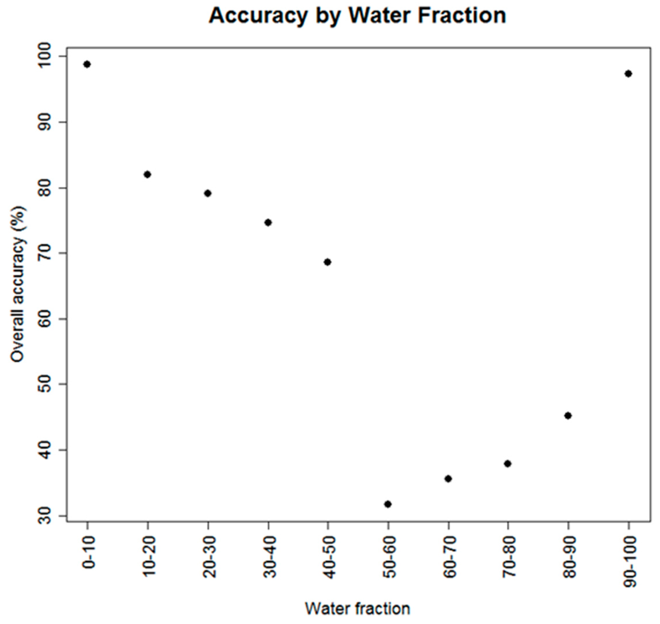
3.2. Assessment—Summer Water Extents vs. Ortho Water Fractions
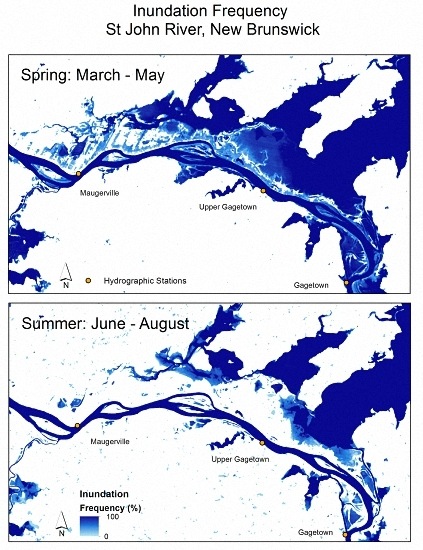
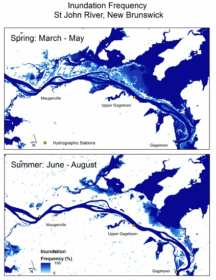
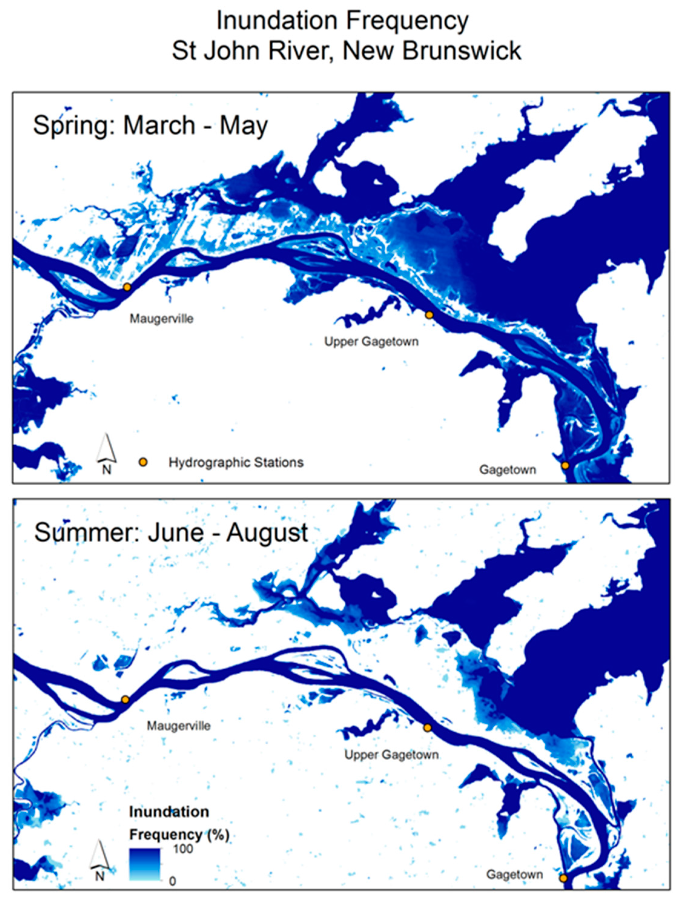
3.3. Inundation Frequency
4. Discussion
5. Conclusions
Acknowledgments
Conflicts of Interest
References
- Intergovernmental Panel on Climate Change (IPCC). Climate Change 2014: Synthesis Report. Contribution of Working Groups I, II and III to the Fifth Assessment Report of the Intergovernmental Panel on Climate Change; Pachauri, R.K., Meyer, L.A., Eds.; IPCC: Geneva, Switzerland, 2014. [Google Scholar]
- Das, S.; Millington, N.; Simonovic, S.P. Distribution choice for the assessment of design rainfall for the city of London (Ontario, Canada) under climate change. Can. J. Civ. Eng. 2013, 40, 121–129. [Google Scholar] [CrossRef]
- Environment and Climate Change Canada, Canada’s Top Ten Weather Stories 2013. Available online: http://ec.gc.ca/meteo-weather/default.asp?lang=En&n=5BA5EAFC-1&offset=2&toc=hide (accessed on 14 September 2016).
- Government of New Brunswick Flood history Database. Available online: http://www.elgegl.gnb.ca/0001/en/Flood/Search (accessed on 12 September 2016).
- Anselmo, V.; Galeati, G.; Palmieri, S.; Rossi, U.; Todini, E. Flood risk assessment using an integrated hydrological and hydraulic modelling approach: A case study. J. Hydrol. 1996, 175, 533–554. [Google Scholar] [CrossRef]
- Wheater, H.S.; Chandler, R.E.; Onof, C.J.; Isham, V.S.; Bellone, E.; Yang, C.; Lekkas, D.; Lourmas, G.; Segond, M.-L. Spatial-temporal rainfall modelling for flood risk estimation. Stoch. Environ. Res. Risk Assess. 2005, 19, 403–416. [Google Scholar] [CrossRef]
- Madsen, H.; Jakobsen, F. Cyclone induced storm surge and flood forecasting in the northern Bay of Bengal. Coast. Eng. 2004, 51, 277–296. [Google Scholar] [CrossRef]
- Bates, P.D.; Dawson, R.J.; Hall, J.W.; Horritt, M.S.; Nicholls, R.J.; Wicks, J.; Hassan, M.A.A.M. Simplified two-dimensional numerical modelling of coastal flooding and example applications. Coast. Eng. 2005, 52, 793–810. [Google Scholar] [CrossRef]
- Hunter, N.M.; Bates, P.D.; Horritt, M.S.; Wilson, M.D. Simple spatially-distributed models for predicting flood inundation: A review. Geomorphology 2007, 90, 208–225. [Google Scholar] [CrossRef]
- Sampson, C.C.; Smith, A.M.; Bates, P.D.; Neal, J.C.; Alfieri, L.; Freer, J.E. A high-resolution global flood hazard model. Water Resour. Res. 2015, 51, 7358–7381. [Google Scholar] [CrossRef] [PubMed]
- Morena, L.C.; James, K.V.; Beck, J. An introduction to the RADARSAT-2 mission. Can. J. Remote Sens. 2004, 30, 221–234. [Google Scholar] [CrossRef]
- Bolanos, S.; Stiff, D.; Brisco, B.; Pietroniro, A. Operational surface water detection and monitoring using RADARSAT 2. Remote Sens. 2016, 8, 285. [Google Scholar] [CrossRef]
- White, L.; Brisco, B.; Dabboor, M.; Schmitt, A.; Pratt, A. A Collection of SAR Methodologies for Monitoring Wetlands. Remote Sens. 2015, 7, 7615–7645. [Google Scholar] [CrossRef]
- Qi, S.; Brown, D.G.; Tian, Q.; Jiang, L.; Zhao, T.; Bergen, K.M. Inundation Extent and Flood Frequency Mapping Using LANDSAT Imagery and Digital Elevation Models. GISci. Remote Sens. 2009, 46, 101–127. [Google Scholar] [CrossRef]
- Thomas, R.F.; Kingsford, R.T.; Lu, Y.; Hunter, S.J. Landsat mapping of annual inundation (1979–2006) of the Macquarie Marshes in semi-arid Australia. Int. J. Remote Sens. 2011, 32, 4545–4569. [Google Scholar] [CrossRef]
- Mueller, N.; Lewis, A.; Roberts, D.; Ring, S.; Melrose, R.; Sixsmith, J.; Lymburner, L.; McIntyre, A.; Tan, P.; Curnow, S.; Ip, A. Water observations from space: Mapping surface water from 25 years of Landsat imagery across Australia. Remote Sens. Environ. 2016, 174, 341–352. [Google Scholar] [CrossRef]
- Chander, G.; Markham, B.L.; Helder, D.L. Summary of current radiometric calibration coefficients for Landsat MSS, TM, ETM+, and EO-1 ALI sensors. Remote Sens. Environ. 2009, 113, 893–903. [Google Scholar] [CrossRef]
- Zhu, Z.; Wang, S.; Woodcock, C.E. Improvement and expansion of the Fmask algorithm: Cloud, cloud shadow, and snow detection for Landsats 4–7, 8, and Sentinel 2 images. Remote Sens. Environ. 2015, 159, 269–277. [Google Scholar] [CrossRef]
- Quinlan, J.R. C4.5: Programs for Machine Learning; Morgan Kaufmann Publishers Inc.: San Francisco, CA, USA, 1993. [Google Scholar]
- Friedl, M.A.; Brodley, C.E. Decision tree classification of land cover from remotely sensed data. Remote Sens. Environ. 1997, 61, 399–409. [Google Scholar] [CrossRef]
- Pal, M.; Mather, P.M. An assessment of the effectiveness of decision tree methods for land cover classification. Remote Sens. Environ. 2003, 86, 554–565. [Google Scholar] [CrossRef]
- Olthof, I.; Fraser, R.H. Detecting Landscape Changes in High Latitude Environments Using Landsat Trend Analysis: 2. Classification. Remote Sens. 2014, 6, 11558–11578. [Google Scholar] [CrossRef]
- Fraser, R.H.; Olthof, I.; Lantz, T.C.; Schmitt, C. UAV photogrammetry for mapping vegetation in the low-Arctic. Arct. Sci. 2016, 2, 79–102. [Google Scholar] [CrossRef]
- Fry, J.; Xian, G.; Jin, S.; Dewitz, J.; Homer, C.; Yang, L.; Barnes, C.; Herold, N.; Wickham, J. Completion of the 2006 National Land Cover Database for the conterminous United States. Photogramm. Eng. Remote Sens. 2011, 77, 858–863. [Google Scholar]
- Machine Learning. Available online: http://www.goodreads.com/work/best_book/206219-machine-learning (accessed on 12 January 2017).
- R Core Team. R: A Language and Environment for Statistical Computing; R Foundation for Statistical Computing: Vienna, Austria, 2014. [Google Scholar]
- Frazier, P.S.; Page, K.J. Water body detection and delineation with Landsat TM data. Photogramm. Eng. Remote Sens. 2000, 66, 1461–1467. [Google Scholar]
- Roach, J.K.; Griffith, B.; Verbyla, D. Comparison of three methods for long-term monitoring of boreal lake area using Landsat TM and ETM+ imagery. Can. J. Remote Sens. 2012, 38, 427–440. [Google Scholar]
- Olthof, I.; Fraser, R.H.; Schmitt, C. Landsat-based mapping of thermokarst lake dynamics on the Tuktoyaktuk Coastal Plain, Northwest Territories, Canada since 1985. Remote Sens. Environ. 2015, 168, 194–204. [Google Scholar] [CrossRef]
- Centre for Topographic Information Customer Support Group. CDED Canadian Digital Elevation Data, Standards and Specifications. Geomatics Canada, Natural Resources Canada. Available online: http://www.pancroma.com/downloads/NRCAN_CDED_specs.pdf (accessed on 10 November 2016).
- Kinsman, N.; Gibbs, A.; Nolan, M. Evaluation of vector coastline features extracted from “Structure from Motion”—Derived elevation data. World Sci. 2015. [Google Scholar] [CrossRef]
- Ackerman, S.; Strabala, K.; Menzel, P.; Frey, R.; Moeller, C.; Gumley, L. Discriminating Clear-Sky from Cloud with MODIS—Algorithm Theoretical Basis Document (MOD35); ATBD Reference Number: ATBD-MOD-06; NASA: Greenbelt, MD, USA, 2010.
- Pekel, J.-F.; Cottam, A.; Gorelick, N.; Belward, A.S. High-resolution mapping of global surface water and its long-term changes. Nature 2016, 540, 418–422. [Google Scholar] [CrossRef] [PubMed]
- Brisco, B.; Short, N.; van der Sanden, J.; Landry, R.; Raymond, D. A semi-automated tool for surface water mapping with RADARSAT-1. Can. J. Remote Sens. 2009, 35, 336–344. [Google Scholar] [CrossRef]
- Hong, S.; Jang, H.; Kim, N.; Sohn, H.-G. Water area extraction using RADARSAT SAR imagery combined with Landsat imagery and terrain information. Sensors 2015, 15, 6652–6667. [Google Scholar] [CrossRef] [PubMed]
- Wulder, M.A.; Hilker, T.; White, J.C.; Coops, N.C.; Masek, J.G.; Pflugmacher, D.; Crevier, Y. Virtual constellations for global terrestrial monitoring. Remote Sens. Environ. 2015, 170, 62–76. [Google Scholar] [CrossRef]


| Reference Data | |||||
|---|---|---|---|---|---|
| Water | Land | Total Classification | User’s Accuracy (%) | ||
| Classification data | Water | 257,470 | 13,576 | 271,046 | 94.99 |
| Land | 14,900 | 802,548 | 817,448 | 98.18 | |
| Total reference | 272,370 | 816,124 | 1,088,494 | ||
| Producer’s accuracy (%) | 94.53 | 98.34 | |||
| Overall accuracy (%) | 97.38 | ||||
| Kappa (%) | 93.02 | ||||
© 2017 by the author. Licensee MDPI, Basel, Switzerland. This article is an open access article distributed under the terms and conditions of the Creative Commons Attribution (CC BY) license ( http://creativecommons.org/licenses/by/4.0/).
Share and Cite
Olthof, I. Mapping Seasonal Inundation Frequency (1985–2016) along the St-John River, New Brunswick, Canada using the Landsat Archive. Remote Sens. 2017, 9, 143. https://doi.org/10.3390/rs9020143
Olthof I. Mapping Seasonal Inundation Frequency (1985–2016) along the St-John River, New Brunswick, Canada using the Landsat Archive. Remote Sensing. 2017; 9(2):143. https://doi.org/10.3390/rs9020143
Chicago/Turabian StyleOlthof, Ian. 2017. "Mapping Seasonal Inundation Frequency (1985–2016) along the St-John River, New Brunswick, Canada using the Landsat Archive" Remote Sensing 9, no. 2: 143. https://doi.org/10.3390/rs9020143