
Analyses of Recent Sediment Surface Dynamic of a Namibian Kalahari Salt Pan Based on Multitemporal Landsat and Hyperspectral Hyperion Data


Abstract
:
1. Introduction
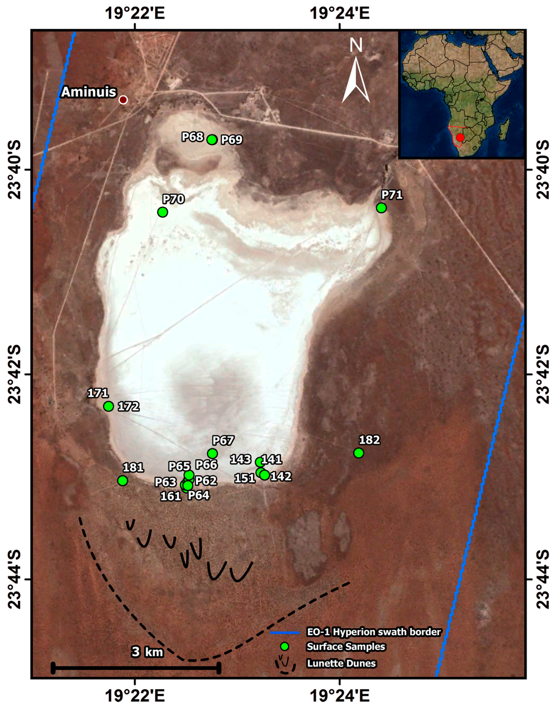
2. Study Area
3. Materials and Methods
3.1. Field and Laboratory Analysis
3.2. Remote Sensing Change Detection Analyses
3.3. Remote Sensing Surface Characterisation
3.3.1. EO-1 Hyperion Mineralogical Mapping
3.3.2. LiDAR Digital Surface Model
4. Results
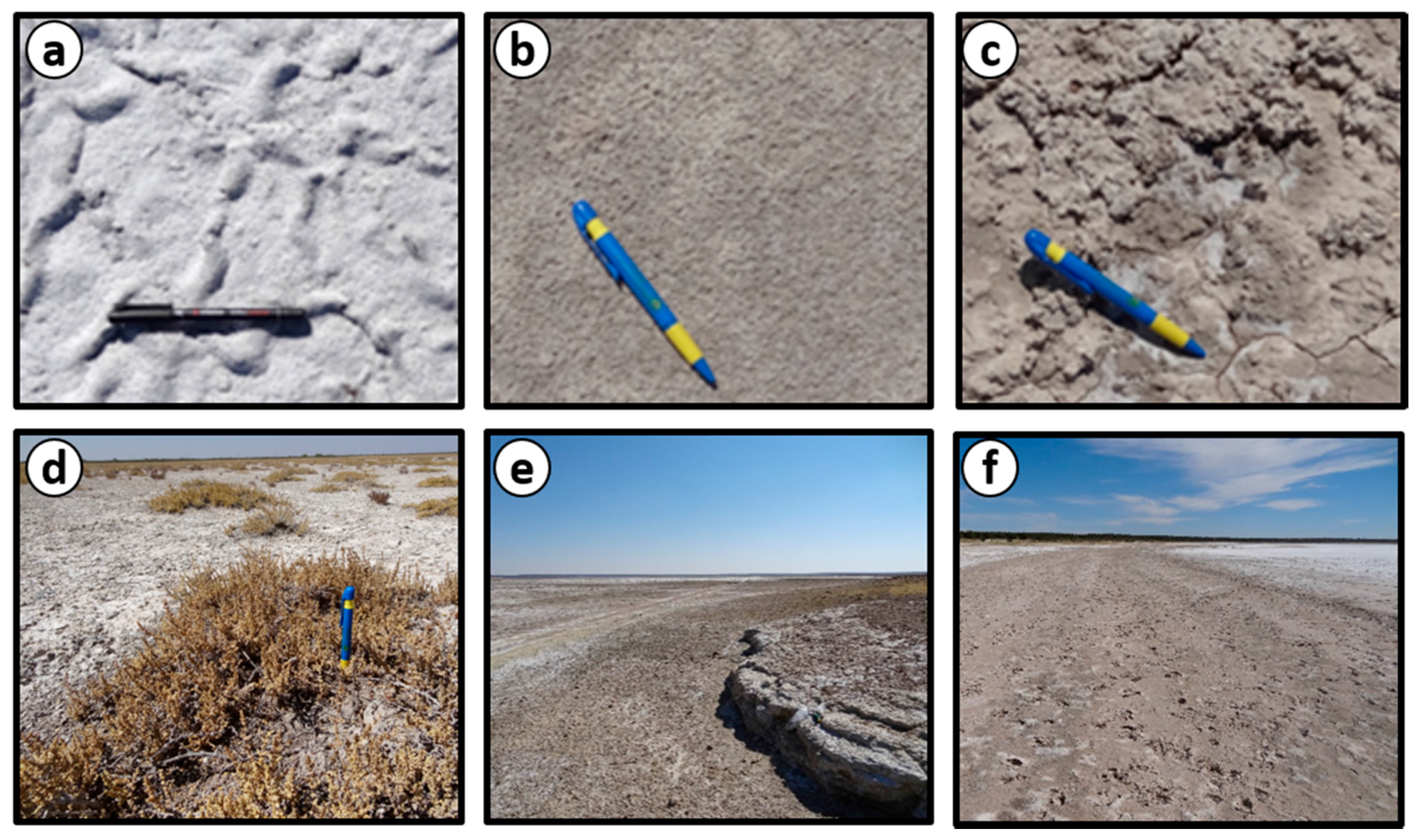
4.1. Field and Laboratory Analysis
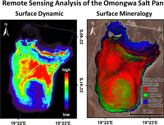
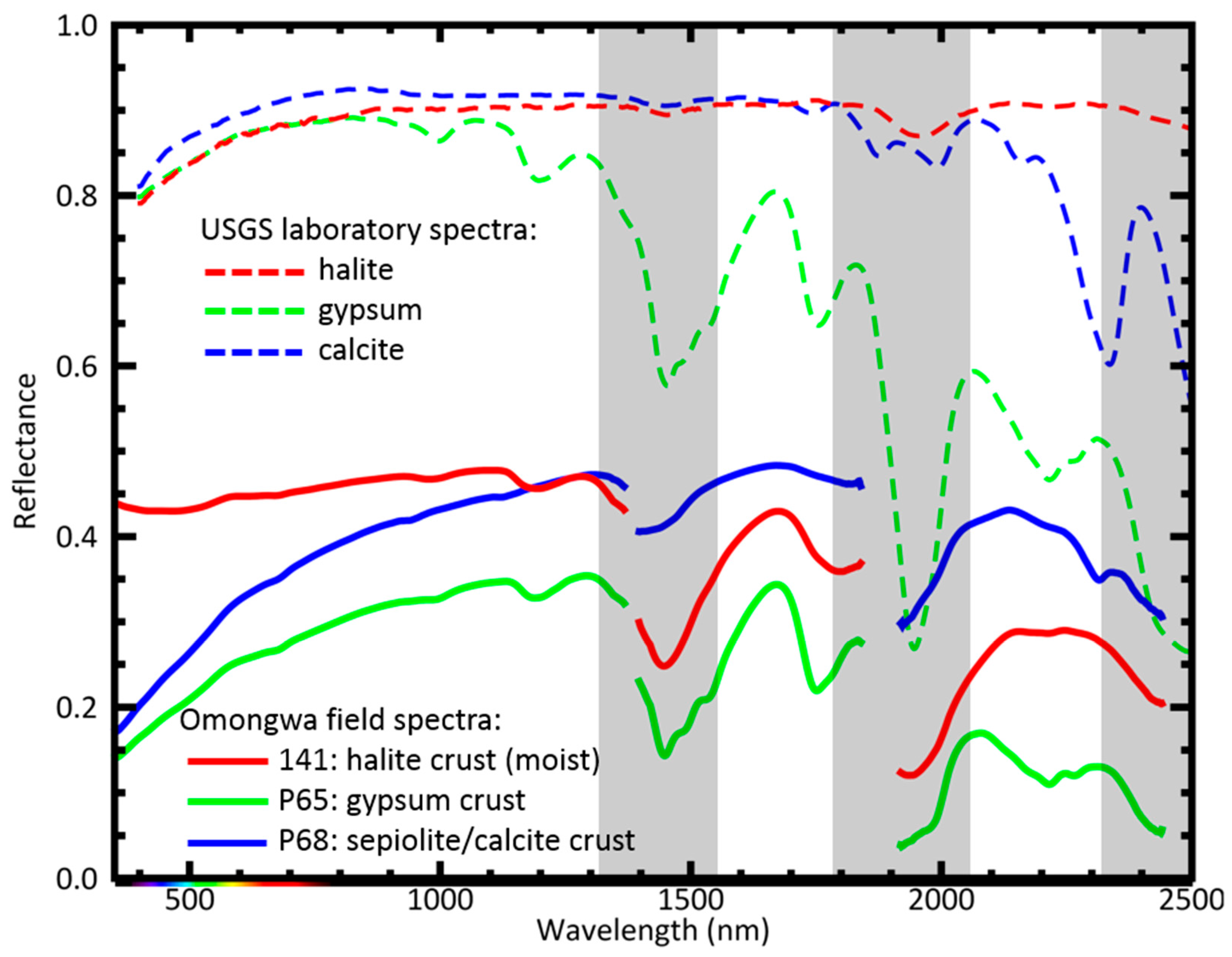
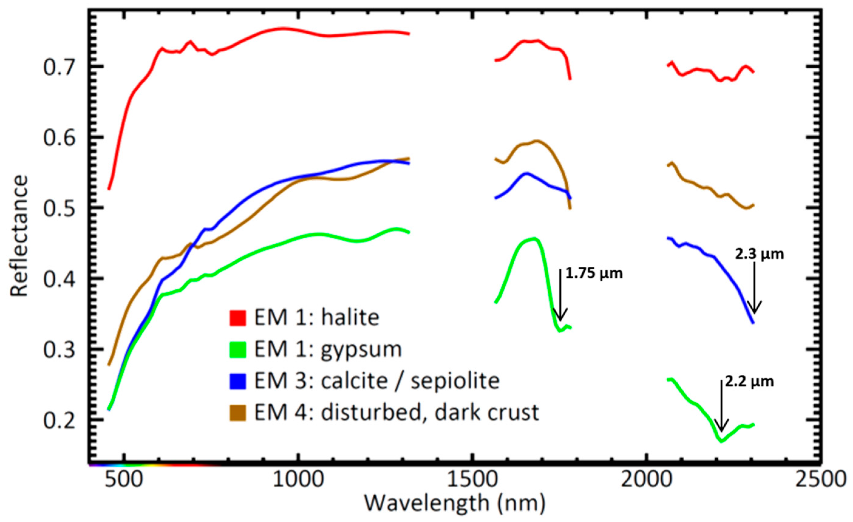
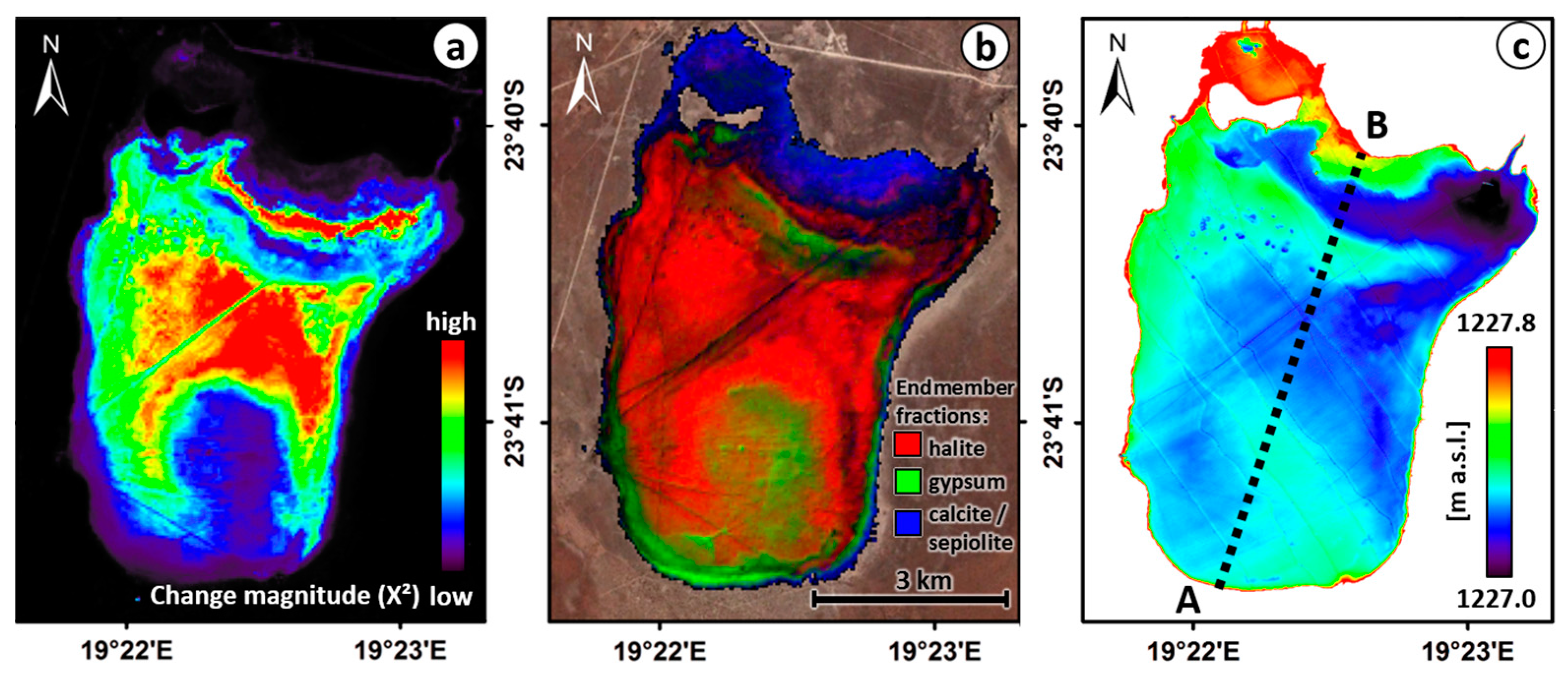
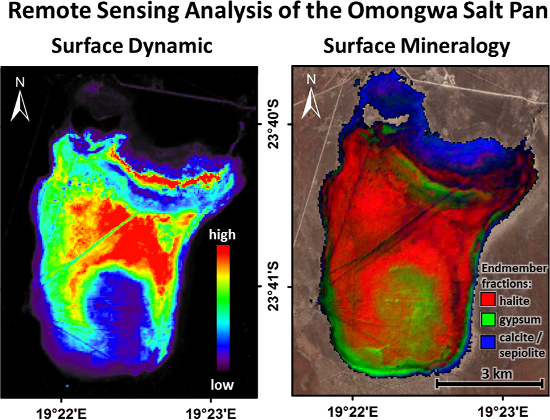
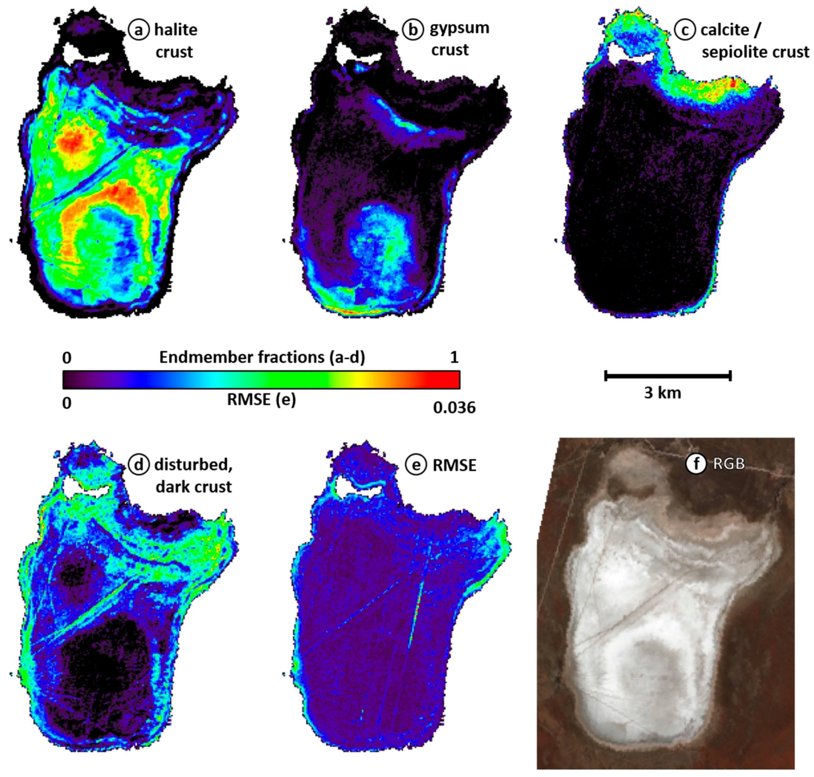
4.2. EO-1 Hyperion Analyses
4.3. Remote Sensing Change Detection Analyses
5. Discussion
5.1. Pan Surface Characterisation
5.2. Interpretation of Pan Surface Processes and Depositional Environment
6. Conclusions
Acknowledgments
Author Contributions
Conflicts of Interest
References
- Millington, A.C.; Drake, N.A.; Townshend, J.R.G.; Quarmby, N.A.; Settle, J.J.; Reading, A.J. Monitoring salt playa dynamics using Thematic Mapper data. IEEE Trans. Geosci. Remote Sens. 1989, 27, 754–761. [Google Scholar] [CrossRef]
- Shaw, P.A.; Bryant, R.G. Pans, Playas and Salt Lakes. In Arid Zone Geomorphology; Thomas, D.S.G., Ed.; John Wiley & Sons, Ltd.: London, UK, 2011; pp. 373–401. [Google Scholar]
- Neal, J.T. Playa surface features as indicators of environment. In Playas and Dried Lakes; Neal, J.T., Ed.; Dowden, Hutchinson & Ross: Stroudsburg, PA, USA, 1975; pp. 363–380. [Google Scholar]
- Rosen, M.R. Paleoclimate and Basin Evolution of Playa Systems; Geological Society of America: Boulder, CO, USA, 1994. [Google Scholar]
- Washington, R.; Todd, M.; Middleton, N.J.; Goudie, A.S. Dust-Storm Source Areas Determined by the Total Ozone Monitoring Spectrometer and Surface Observations. Ann. Assoc. Am. Geogr. 2003, 93, 297–313. [Google Scholar] [CrossRef]
- Prospero, J.M.; Ginoux, P.; Torres, O.; Nicholson, S.E.; Gill, T.E. Environmental Characterization of Global Sources of Atmospheric Soil Dust Identified with the Nimbus 7 Total Ozone Mapping Spectrometer (Toms) Absorbing Aerosol Product. Rev. Geophys. 2002, 40, 1002. [Google Scholar] [CrossRef]
- Vickery, K.J.; Eckardt, F.D.; Bryant, R.G. A sub-basin scale dust plume source frequency inventory for southern Africa, 2005–2008. Geophys. Res. Lett. 2013, 40, 5274–5279. [Google Scholar] [CrossRef]
- Nield, J.M.; Bryant, R.G.; Wiggs, G.F.S.; King, J.; Thomas, D.S.G.; Eckardt, F.D.; Washington, R. The dynamism of salt crust patterns on playas. Geology 2015, 43, 31–34. [Google Scholar] [CrossRef]
- Reynolds, R.L.; Yount, J.C.; Reheis, M.; Goldstein, H.; Chavez, P.; Fulton, R.; Whitney, J.; Fuller, C.; Forester, R.M. Dust emission from wet and dry playas in the Mojave Desert, USA. Earth Surf. Process. Landf. 2007, 32, 1811–1827. [Google Scholar] [CrossRef]
- Buck, B.J.; King, J.; Etyemezian, V. Effects of Salt Mineralogy on Dust Emissions, Salton Sea, California. Soil Sci. Soc. Am. J. 2011, 75, 1971–1985. [Google Scholar] [CrossRef]
- Katra, I.; Lancaster, N. Surface-sediment dynamics in a dust source from spaceborne multispectral thermal infrared data. Remote Sens. Environ. 2008, 112, 3212–3221. [Google Scholar] [CrossRef]
- Thomas, A.D.; Dougill, A.J.; Elliott, D.R.; Mairs, H. Seasonal differences in soil CO2 efflux and carbon storage in Ntwetwe Pan, Makgadikgadi Basin, Botswana. Geoderma 2014, 219–220, 72–81. [Google Scholar] [CrossRef]
- Bryant, R.G. Validated linear mixture modelling of Landsat TM data for mapping evaporite minerals on a playa surface: methods and applications. Int. J. Remote Sens. 1996, 17, 315–330. [Google Scholar] [CrossRef]
- Drake, N.A. Reflectance spectra of evaporite minerals (400–2500 nm): Applications for remote sensing. Int. J. Remote Sens. 1995, 16, 2555–2571. [Google Scholar] [CrossRef]
- Lowenstein, T.K.; Hardie, L.A. Criteria for the recognition of salt-pan evaporites. Sedimentology 1985, 32, 627–644. [Google Scholar] [CrossRef]
- Alanazi, H.A.; Ghrefat, H.A. Spectral Analysis of Multispectral Landsat 7 ETM + and ASTER Data for Mapping Land Cover at Qurayah Sabkha, Northern Saudi Arabia. J. Indian Soc. Remote Sens. 2013, 41, 833–844. [Google Scholar] [CrossRef]
- Li, J.; Menenti, M.; Mousivand, A.; Luthi, S.M. Non-Vegetated Playa Morphodynamics Using Multi-Temporal Landsat Imagery in a Semi-Arid Endorheic Basin: Salar de Uyuni, Bolivia. Remote Sens. 2014, 6, 10131–10151. [Google Scholar] [CrossRef]
- Chapman, J.E.; Rothery, D.A.; Francis, P.W.; Pontual, A. Remote sensing of evaporite mineral zonation in salt flats (salars). Int. J. Remote Sens. 1989, 10, 245–255. [Google Scholar] [CrossRef]
- White, K.; Eckardt, F. Geochemical mapping of carbonate sediments in the Makgadikgadi basin, Botswana using moderate resolution remote sensing data. Earth Surf. Process. Landf. 2006, 31, 665–681. [Google Scholar] [CrossRef]
- Hubbard, B.E.; Crowley, J.K. Mineral mapping on the Chilean–Bolivian Altiplano using co-orbital ALI, ASTER and Hyperion imagery: Data dimensionality issues and solutions. Remote Sens. Environ. 2005, 99, 173–186. [Google Scholar] [CrossRef]
- Kodikara, G.R.L.; Woldai, T.; van Ruitenbeek, F.J.A.; Kuria, Z.; van der Meer, F.; Shepherd, K.D.; van Hummel, G.J. Hyperspectral remote sensing of evaporate minerals and associated sediments in Lake Magadi area, Kenya. Int. J. Appl. Earth Obs. Geoinf. 2012, 14, 22–32. [Google Scholar] [CrossRef]
- Green, R.O.; Pavri, B.E.; Chrien, T.G. On-orbit radiometric and spectral calibration characteristics of EO-1 Hyperion derived with an underflight of AVIRIS and in situ measurements at Salar de Arizaro, Argentina. IEEE Trans. Geosci. Remote Sens. 2003, 41, 1194–1203. [Google Scholar] [CrossRef]
- Thome, K.J.; Biggar, S.F.; Wisniewski, W. Cross comparison of EO-1 sensors and other Earth resources sensors to Landsat-7 ETM+ using Railroad Valley Playa. IEEE Trans. Geosci. Remote Sens. 2003, 41, 1180–1188. [Google Scholar] [CrossRef]
- Dutkiewicz, A.; Lewis, M.; Ostendorf, B. The Suitability of Airborne Hyperspectral Imagery for Mapping Surface Indicators of Salinity in Dryland Farming Area. In Remote Sensing of Soil Salinization: Impact on Land Management; CRC Press: Boca Raton, FL, USA, 2008; pp. 93–112. [Google Scholar]
- Kruse, F.A.; Boardman, J.W.; Huntington, J.F. Comparison of airborne hyperspectral data and EO-1 Hyperion for mineral mapping. IEEE Trans. Geosci. Remote Sens. 2003, 41, 1388–1400. [Google Scholar] [CrossRef]
- Crowley, J.K.; Hubbard, B.E.; Mars, J.C. Analysis of potential debris flow source areas on Mount Shasta, California, by using airborne and satellite remote sensing data. Remote Sens. Environ. 2003, 87, 345–358. [Google Scholar] [CrossRef]
- Mees, F. Distribution patterns of gypsum and kalistrontite in a dry lake basin of the southwestern Kalahari (Omongwa pan, Namibia). Earth Surf. Process. Landf. 1999, 24, 731–744. [Google Scholar] [CrossRef]
- Mees, F.; Van Ranst, E. Micromorphology of sepiolite occurrences in recent lacustrine deposits affected by soil development. Soil Res. 2011, 49, 547–557. [Google Scholar] [CrossRef]
- Kautz, K.; Parada, H. Sepiolote formation in a pan of the Kalahari, South West Africa. J. Mineral. Geochem. 1976, 12, 545–559. [Google Scholar]
- Lancaster, N. Pans in the southwestern Kalahari. A preliminary report. Palaeoecol. Afr. 1986, 17, 59–68. [Google Scholar]
- Köppen, W.P.; Geiger, R. Handbuch der Klimatologie in fünf bänden; Verlag von Gebrüder Borntraeger: Berlin, Germany, 1930. [Google Scholar]
- Atlas of Namibia Project Atlas of Namibia Project (2002) Directorate of Environmental Affairs, Minitry of Environment and Tourism. Available online: http://www.uni-koeln.de/sfb389/e/e1/download/atlas_namibia/e1_download_climate_e.htm (accessed on 24 November 2015).
- Thomas, D.; Shaw, P.A. The Kalahari Environment; Cambridge University Press: Cambridge, UK, 1991. [Google Scholar]
- Van Veleen, M.; Baker, T. Feasibility Study of the Potential for Sustainable Water Resources Development in the Molopo-Nossob Watercourse, 2009. Available online: http://iwlearn.net/resources/documents/3516 (accessed on 16 February 2017).
- Miller, R.M. The Geology of Namibia: Upper Palaeozoic to Cenozoic; Ministry of Mines and Energy, Geological Survey of Namibia: Windhoek, Namibia, 2008.
- Mees, F. The nature of calcareous deposits along pan margins in eastern central Namibia. Earth Surf. Process. Landf. 2002, 27, 719–735. [Google Scholar] [CrossRef]
- SACS (South African Committee for Stratigraphy). Stratigraphy of South Africa. Part 1: Lithostratigraphy of the Republic of South Africa, South West Africa/Namibia and the Republics of Bophuthatswana, Transkei and Venda; Geological Survey of South Africa: Johannesburg, South Africa, 1980. [Google Scholar]
- JICA Study Team. The Study on the Groundwater Potential Evaluation and Management Plan in the Southeast Kalahari(Stampriet) Artesian Basin in the Republic of Namibia: Final Report: Data Book; Pacific Consultants International: Tokyo, Japan, 2002. [Google Scholar]
- FAO. World Reference Base for Soil Resources 2006. A Framework for International Classification, Correlation and Communication; Word Soil Resources Report 103; IUSS-ISRIC-FAO: Rome, Italy, 2006. [Google Scholar]
- Stone, A.E.C.; Edmunds, W.M. Sand, salt and water in the Stampriet Basin, Namibia: Calculating unsaturated zone (Kalahari dunefield) recharge using the chloride mass balance approach. Water SA 2012, 38, 367–378. [Google Scholar] [CrossRef]
- Local Office of the Namibian Ministries of Agriculture, Basic Education and Health. Personal communication, 2015.
- ASD Inc. Field Spec—User Manual 2010. Available online: http://support.asdi.com/Document/Viewer.aspx?id=108 (accessed on 16 February 2017).
- Soil Quality—Determination of Particle Size Distribution in Mineral Soil Material—Method by Sieving and Sedimentation (ISO 11277:1998 + ISO 11277:1998 Corrigendum 1:2002) 2002. Available online: http://www.iso.org/iso/catalogue_detail.htm?csnumber=54151 (accessed on 16 February 2017).
- Soil Quality—Determination of the Specific Electrical Conductivity (ISO 11265:1994 + ISO 11265:1994/Corr.1:1996) 1997. Available online: http://www.iso.org/iso/catalogue_detail.htm?csnumber=19243 (accessed on 16 February 2017).
- EarthExplorer. Available online: http://earthexplorer.usgs.gov/ (accessed on 16 February 2017).
- Chander, G.; Markham, B.L.; Helder, D.L. Summary of current radiometric calibration coefficients for Landsat MSS, TM, ETM+, and EO-1 ALI sensors. Remote Sens. Environ. 2009, 113, 893–903. [Google Scholar] [CrossRef]
- Masek, J.G.; Vermote, E.F.; Saleous, N.E.; Wolfe, R.; Hall, F.G.; Huemmrich, K.F.; Gao, F.; Kutler, J.; Lim, T.-K. LEDAPS Calibration, Reflectance, Atmospheric Correction Preprocessing Code, version 2, 2013. Available online: https://daac.ornl.gov/cgi-bin/dsviewer.pl?ds_id=1146 (accessed on 16 February 2017).
- Masek, J.G.; Vermote, E.F.; Saleous, N.E.; Wolfe, R.; Hall, F.G.; Huemmrich, K.F.; Gao, F.; Kutler, J.; Lim, T.-K. A Landsat surface reflectance dataset for North America, 1990. IEEE Geosci. Remote Sens. Lett. 2006, 3, 68–72. [Google Scholar] [CrossRef]
- United States Geological Survey (USGS). Product Guide. Provisional Landsat 8 Surface Reflectance Product; United States Geological Survey: Boulder, CO, USA, 2015; p. 27.
- Kaufman, Y.J.; Wald, A.E.; Remer, L.A.; Gao, B.-C.; Li, R.-R.; Flynn, L. The MODIS 2.1-μm channel-correlation with visible reflectance for use in remote sensing of aerosol. IEEE Trans. Geosci. Remote Sens. 1997, 35, 1286–1298. [Google Scholar] [CrossRef]
- Maiersperger, T.K.; Scaramuzza, P.L.; Leigh, L.; Shrestha, S.; Gallo, K.P.; Jenkerson, C.B.; Dwyer, J.L. Characterizing LEDAPS surface reflectance products by comparisons with AERONET, field spectrometer, and MODIS data. Remote Sens. Environ. 2013, 136, 1–13. [Google Scholar] [CrossRef]
- Vermote, E.; Justice, C.; Claverie, M.; Franch, B. Preliminary analysis of the performance of the Landsat 8/OLI land surface reflectance product. Remote Sens. Environ. 2016, 185, 46–56. [Google Scholar] [CrossRef]
- Xu, H. Modification of normalised difference water index (NDWI) to enhance open water features in remotely sensed imagery. Int. J. Remote Sens. 2006, 27, 3025–3033. [Google Scholar] [CrossRef]
- Li, W.; Du, Z.; Ling, F.; Zhou, D.; Wang, H.; Gui, Y.; Sun, B.; Zhang, X. A Comparison of Land Surface Water Mapping Using the Normalized Difference Water Index from TM, ETM+ and ALI. Remote Sens. 2013, 5, 5530–5549. [Google Scholar] [CrossRef]
- Verbesselt, J.; Hyndman, R.; Newnham, G.; Culvenor, D. Detecting trend and seasonal changes in satellite image time series. Remote Sens. Environ. 2010, 114, 106–115. [Google Scholar] [CrossRef]
- Pesaran, M.H.; Timmermann, A. Market timing and return prediction under model instability. J. Empir. Financ. 2002, 9, 495–510. [Google Scholar] [CrossRef]
- DeVries, B.; Verbesselt, J.; Kooistra, L.; Herold, M. Robust monitoring of small-scale forest disturbances in a tropical montane forest using Landsat time series. Remote Sens. Environ. 2015, 161, 107–121. [Google Scholar] [CrossRef]
- Verbesselt, J.; Zeileis, A.; Herold, M. Near real-time disturbance detection using satellite image time series. Remote Sens. Environ. 2012, 123, 98–108. [Google Scholar] [CrossRef]
- Nielsen, A.A. The Regularized Iteratively Reweighted MAD Method for Change Detection in Multi- and Hyperspectral Data. IEEE Trans. Image Process. 2007, 16, 463–478. [Google Scholar] [CrossRef] [PubMed] [Green Version]
- Liao, M.; Zhu, P.; Gong, J. Multivariate Change Detection Based on Canonical Transformation. J. Remote Sens. 2000, 4, 197–201. [Google Scholar]
- Pathak, S. New Change Detection Techniques to monitor land cover dynamics in mine environment. ISPRS Int. Arch. Photogramm. Remote Sens. Spat. Inf. Sci. 2014, XL-8, 875–879. [Google Scholar] [CrossRef]
- Mezned, N.; Dkhala, B.; Abdeljaouad, S. Multi temporal and multi spectral images based change detection of mine wastes in Northern Tunisia. In Proceedings of the 2015 IEEE International Geoscience and Remote Sensing Symposium (IGARSS), Milan, Italy, 26–31 July November 2015; pp. 3426–3429.
- Colditz, R.R.; Llamas, R.M.; Gebhardt, S.; Wehrmann, T.; Equihua, J. Comparison of change detection techniques for the Yucatan peninsula using Landsat image time series. In Proceedings of the 2015 IEEE International Geoscience and Remote Sensing Symposium (IGARSS), Milan, Italy, 26–31 July 2015; pp. 1650–1653.
- Ma, Y.; Chen, F.; Liu, J.; He, Y.; Duan, J.; Li, X. An Automatic Procedure for Early Disaster Change Mapping Based on Optical Remote Sensing. Remote Sens. 2016, 8, 272. [Google Scholar] [CrossRef]
- Hoja, D.; Krauss, T.; Reinartz, P. Detailed damage assessment after the Haiti earthquake. In Earth Observation of Global Changes (EOGC); Springer: Berlin, Germany, 2013; pp. 193–204. [Google Scholar]
- Zhang, L.; Liao, M.; Yang, L.; Lin, H. Remote sensing change detection based on canonical correlation analysis and contextual Bayes decision. Photogramm. Eng. Remote Sens. 2007, 73, 311–318. [Google Scholar] [CrossRef]
- Nielsen, A.A. Analysis of Regularly and Irregularly Sampled Spatial, Multivariate, and Multi-Temporal Data; Technical University of Denmark: Lyngby, Denmark, 1994. [Google Scholar]
- Coppin, P.; Jonckheere, I.; Nackaerts, K.; Muys, B.; Lambin, E. Digital change detection methods in ecosystem monitoring: A review. Int. J. Remote Sens. 2004, 25, 1565–1596. [Google Scholar] [CrossRef]
- Nielsen, A.A.; Conradsen, K.; Simpson, J.J. Multivariate Alteration Detection (MAD) and MAF Postprocessing in Multispectral, Bitemporal Image Data: New Approaches to Change Detection Studies. Remote Sens. Environ. 1998, 64, 1–19. [Google Scholar] [CrossRef]
- Ju, J.; Roy, D.P. The availability of cloud-free Landsat ETM+ data over the conterminous United States and globally. Remote Sens. Environ. 2008, 112, 1196–1211. [Google Scholar] [CrossRef]
- Aghamohamadnia, M.; Abedini, A. A morphology-stitching method to improve Landsat SLC-off images with stripes. Geod. Geodyn. 2014, 5, 27–33. [Google Scholar] [CrossRef]
- Chen, J.; Zhu, X.; Vogelmann, J.E.; Gao, F.; Jin, S. A simple and effective method for filling gaps in Landsat ETM+ SLC-off images. Remote Sens. Environ. 2011, 115, 1053–1064. [Google Scholar] [CrossRef]
- Alexandridis, T.K.; Cherif, I.; Kalogeropoulos, C.; Monachou, S.; Eskridge, K.; Silleos, N. Rapid error assessment for quantitative estimations from Landsat 7 gap-filled images. Remote Sens. Lett. 2013, 4, 920–928. [Google Scholar] [CrossRef]
- Bédard, F.; Reichert, G.; Dobbins, R.; Trépanier, I. Evaluation of segment-based gap-filled Landsat ETM+ SLC-off satellite data for land cover classification in southern Saskatchewan, Canada. Int. J. Remote Sens. 2008, 29, 2041–2054. [Google Scholar] [CrossRef]
- Canty, M.J. Image Analysis, Classification and Change Detection in Remote Sensing: With Algorithms for ENVI/IDL and Python, 3rd ed.; CRC Press: Boca Raton, FL, USA, 2014. [Google Scholar]
- Canty, M.J.; Nielsen, A.A. Linear and kernel methods for multivariate change detection. Comput. Geosci. 2012, 38, 107–114. [Google Scholar] [CrossRef]
- Nielsen, A.A.; Hecheltjen, A.; Thonfeld, F.; Canty, M.J. Automatic change detection in RapidEye data using the combined MAD and kernel MAF methods. In Proceedings of the IGARSS 2010—2010 IEEE International Geoscience and Remote Sensing Symposium, Honolulu, HI, USA, 25–30 July 2010; pp. 3078–3081.
- Liang, W.; Hoja, D.; Schmitt, M.; Stilla, U. Change Detection for Reconstruction Monitoring based on Very High Resolution Optical Data, 2011. Available online: http://elib.dlr.de/69997/1/WenjingLiang_jurse2011_changedetection_word.pdf (accessed on 16 February 2017).
- Pearlman, J.S.; Barry, P.S.; Segal, C.C.; Shepanski, J.; Beiso, D.; Carman, S.L. Hyperion, a space-based imaging spectrometer. IEEE Trans. Geosci. Remote Sens. 2003, 41, 1160–1173. [Google Scholar] [CrossRef]
- Rogass, C.; Guanter, L.; Mielke, C.; Scheffler, D.; Boesche, N.K.; Lubitz, C.; Brell, M.; Spengler, D.; Segl, K. An automated processing chain for the retrieval of georeferenced reflectance data from hyperspectral EO-1 HYPERION acquisitions. In Proceedings of the EARSeL 34th Symposium, Warsaw, Poland, 16–20 June 2014.
- Guanter, L.; Segl, K.; Sang, B.; Alonso, L.; Kaufmann, H.; Moreno, J. Scene-based spectral calibration assessment of high spectral resolution imaging spectrometers. Opt. Express 2009, 17, 11594. [Google Scholar] [CrossRef] [PubMed]
- Guanter, L.; Richter, R.; Kaufmann, H. On the application of the MODTRAN4 atmospheric radiative transfer code to optical remote sensing. Int. J. Remote Sens. 2009, 30, 1407–1424. [Google Scholar] [CrossRef]
- Van der Linden, S.; Rabe, A.; Held, M.; Jakimow, B.; Leitão, P.J.; Okujeni, A.; Schwieder, M.; Suess, S.; Hostert, P. The EnMAP-Box—A Toolbox and Application Programming Interface for EnMAP Data Processing. Remote Sens. 2015, 7, 11249–11266. [Google Scholar] [CrossRef]
- Harris Geospatial Solutions Linear Spectral Unmixing (Using ENVI). Available online: http://www.exelisvis.com/docs/LinearSpectralUnmixing.html (accessed on 4 February 2016).
- Mielke, C.; Muedi, T.; Papenfuss, A.; Boesche, N.K.; Rogass, C.; Gauert, C.D.K.; Altenberger, U.; de Wit, M.J. Multi- and hyperspectral spaceborne remote sensing of the Aggeneys base metal sulphide mineral deposit sites in the Lower Orange River region, South Africa. S. Afr. J. Geol. 2016, 119, 63–76. [Google Scholar] [CrossRef]
- Mielke, C.; Rogass, C.; Boesche, N.; Segl, K.; Altenberger, U. EnGeoMAP 2.0—Automated Hyperspectral Mineral Identification for the German EnMAP Space Mission. Remote Sens. 2016, 8, 127. [Google Scholar] [CrossRef]
- Adams, J.B.; Smith, M.O.; Johnson, P.E. Spectral mixture modeling: A new analysis of rock and soil types at the Viking Lander 1 Site. J. Geophys. Res. Solid Earth 1986, 91, 8098–8112. [Google Scholar] [CrossRef]
- Boardman, J.W.; Kruse, F.A. Automated spectral analysis: A geological example using AVIRIS data, northern Grapevine Mountains, Nevada. In Proceedings of the 10th Thematic Conference on Geologic Remote Sensing, Ann Arbor, MI, USA, 9–12 May 1994; pp. 1407–1418.
- Tompkins, S. Optimization of endmembers for spectral mixture analysis. Remote Sens. Environ. 1997, 59, 472–489. [Google Scholar] [CrossRef]
- Boardman, J.W. Automating Spectral Unmixing of AVIRIS Data Using Convex Geometry Concepts, 1993. Available online: https://ntrs.nasa.gov/search.jsp?R=19950017428 (accessed on 16 February 2017).
- Shrestha, D.P.; Margate, D.E.; van der Meer, F.; Anh, H.V. Analysis and classification of hyperspectral data for mapping land degradation: An application in southern Spain. Int. J. Appl. Earth Obs. Geoinf. 2005, 7, 85–96. [Google Scholar] [CrossRef]
- Garcia-Haro, F.J.; Gilabert, M.A.; Melia, J. Linear spectral mixture modelling to estimate vegetation amount from optical spectral data. Int. J. Remote Sens. 1996, 17, 3373–3400. [Google Scholar] [CrossRef]
- Kruse, F.; Lefkoff, A.; Dietz, J. Expert System-Based Mineral Mapping in Northern Death-Valley, California Nevada, Using the Airborne Visible Infrared Imaging Spectrometer (aviris). Remote Sens. Environ. 1993, 44, 309–336. [Google Scholar] [CrossRef]
- Chabrillat, S.; Pinet, P.C.; Ceuleneer, G.; Johnson, P.E.; Mustard, J.F. Ronda peridotite massif: Methodology for its geological mapping and lithological discrimination from airborne hyperspectral data. Int. J. Remote Sens. 2000, 21, 2363–2388. [Google Scholar] [CrossRef]
- Metternicht, G.I.; Fermont, A. Estimating erosion surface features by linear mixture modeling. Remote Sens. Environ. 1998, 64, 254–265. [Google Scholar] [CrossRef]
- Dennison, P.E.; Roberts, D.A. Endmember selection for multiple endmember spectral mixture analysis using endmember average RMSE. Remote Sens. Environ. 2003, 87, 123–135. [Google Scholar] [CrossRef]
- Farifteh, J.; van der Meer, F.; van der Meijde, M.; Atzberger, C. Spectral characteristics of salt-affected soils: A laboratory experiment. Geoderma 2008, 145, 196–206. [Google Scholar] [CrossRef]
- Green, A.A.; Berman, M.; Switzer, P.; Craig, M.D. A transformation for ordering multispectral data in terms of image quality with implications for noise removal. IEEE Trans. Geosci. Remote Sens. 1988, 26, 65–74. [Google Scholar] [CrossRef]
- Boardman, J.W.; Kruse, F.A.; Green, R.O. Mapping Target Signatures via Partial Unmixing of AVIRIS Data, 1995. Available online: https://ntrs.nasa.gov/search.jsp?R=19950027316 (accessed on 16 February 2017).
- Dimap-Spectral GmbH—Digital Mapping. Available online: http://www.dimap.asia/ (accessed on 16 February 2017).
- Hunt, G.R.; Salisbury, J.W.; Lenhoff, C.J. Visible and near infrared spectra of minerals and rocks, IV Sulphides and sulphates. Mod. Geol. 1971, 3, 121–132. [Google Scholar]
- Clark, R.N.; Swayze, G.A.; Wise, R.; Livo, E.; Hoefen, T.M.; Kokaly, R.F.; Sutley, S.J. USGS Digital Spectral Library splib06a: U.S. Geological Survey, Digital Data Series 231. Available online: http://speclab.cr.usgs.gov/spectral.lib06 (accessed on 16 February 2017).
- Howari, F.M.; Goodell, P.C.; Miyamoto, S. Spectral properties of salt crusts formed on saline soils. J. Environ. Qual. 2002, 31, 1453–1461. [Google Scholar] [CrossRef] [PubMed]
- Khayamim, F.; Wetterlind, J.; Khademi, H.; Robertson, J.; Faz Cano, A.; Stenberg, B. Using visible and near infrared spectroscopy to estimate carbonates and gypsum in soils in arid and subhumid regions of Isfahan, Iran. J. Infrared Spectrosc. 2015, 23, 155. [Google Scholar] [CrossRef]
- Ghosh, G.; Kumar, S.; Saha, S.K. Hyperspectral Satellite Data in Mapping Salt-Affected Soils Using Linear Spectral Unmixing Analysis. J. Indian Soc. Remote Sens. 2012, 40, 129–136. [Google Scholar] [CrossRef]
- Zhang, X.; Shang, K.; Cen, Y.; Shuai, T.; Sun, Y. Estimating ecological indicators of karst rocky desertification by linear spectral unmixing method. Int. J. Appl. Earth Obs. Geoinf. 2014, 31, 86–94. [Google Scholar] [CrossRef]
- Baddock, M.C.; Zobeck, T.M.; Van Pelt, R.S.; Fredrickson, E.L. Dust emissions from undisturbed and disturbed, crusted playa surfaces: Cattle trampling effects. Aeolian Res. 2011, 3, 31–41. [Google Scholar] [CrossRef]
- Metternicht, G.; Zinck, J. Remote sensing of soil salinity: potentials and constraints. Remote Sens. Environ. 2003, 85, 1–20. [Google Scholar] [CrossRef]
- Nield, J.M.; Wiggs, G.F.S.; King, J.; Bryant, R.G.; Eckardt, F.D.; Thomas, D.S.G.; Washington, R. Climate-surface–pore-water interactions on a salt crusted playa: Implications for crust pattern and surface roughness development measured using terrestrial laser scanning. Earth Surf. Process. Landf. 2016, 41, 738–753. [Google Scholar] [CrossRef]
- Chivas, A.R. Chapter 10 Terrestrial Evaporites. In Geochemical Sediments and Landscapes; Nash, D.J., McLaren, S.J., Eds.; RGS-IBG Book Series; Blackwell Pub.: Malden, MA, USA, 2007; pp. 330–364. [Google Scholar]
- Warren, J.K. Evaporites: A Geological Compendium; Springer: Berlin, Germany, 2016. [Google Scholar]
- Smith, M.; Compton, J.S. Origin and evolution of major salts in the Darling pans, Western Cape, South Africa. Appl. Geochem. 2004, 19, 645–664. [Google Scholar] [CrossRef]
- Jones, B.F. The hydrology and Mineralogy of Deep Springs Lake, Inyo County, California; Professional Paper; U.S. Govt. Print. Off.: Washington, USA, 1965.
- Bryant, R.G. The Sedimentology and Geochemistry of Non-Marine Evaporites on the Chott el Djerid, Using Both Ground and Remotely Sensed Data; University of Reading: Reading, UK, 1993. [Google Scholar]
- Guanter, L.; Kaufmann, H.; Segl, K.; Foerster, S.; Rogass, C.; Chabrillat, S.; Kuester, T.; Hollstein, A.; Rossner, G.; Chlebek, C.; et al. The EnMAP Spaceborne Imaging Spectroscopy Mission for Earth Observation. Remote Sens. 2015, 7, 8830–8857. [Google Scholar] [CrossRef]


| Label | Mineralogy (bulk XRD) Semi-Quantitative Estimates (%) | pH | EC (dS/m) | Grain Size (%) | |||||||
|---|---|---|---|---|---|---|---|---|---|---|---|
| Quartz | Halite | Gypsum | Calcite | Sepiolite | Dolomite | Clay | Silt | Sand | |||
| P62 | 79 | - | 21 | - | - | - | 7.9 | 1.9 | 2 | 3 | 95 |
| P63 | 19 | 5 | 75 | - | - | - | 8.6 | 17.6 | 1 | 4 | 95 |
| P64 | 17 | 36 | 47 | - | - | - | - | - | - | - | - |
| P65 | 3 | 14 | 83 | - | - | - | 8.5 | 42.3 | 5 | 4 | 91 |
| P66 | 13 | 41 | 44 | - | 1 | - | - | - | - | - | - |
| P67 | 3 | 46 | 45 | - | 5 | - | 8.4 | 80.7 | 4 | 40 | 56 |
| P68 | 36 | 3 | - | 45 | 16 | - | 8.3 | 10.8 | 4 | 37 | 59 |
| P69 | 28 | 15 | - | 41 | 15 | - | 8.7 | 36.5 | 8 | 39 | 53 |
| P70 | 32 | 16 | 26 | 15 | 11 | - | 8.6 | 33.7 | 2 | 34 | 64 |
| P71 | 26 | 7 | - | 47 | 6 | 14 | - | - | - | - | - |
| 141 | 1 | 94 | 3 | - | - | - | - | - | - | - | - |
| 142 | 63 | 9 | 15 | 7 | 5 | - | 8.8 | 23.4 | 7 | 24 | 69 |
| 143 | 1 | 52 | 38 | 4 | 5 | - | 8.3 | 129.7 | 6 | 73 | 21 |
| 151 | 64 | 21 | 7 | 9 | - | - | 9.1 | 48.2 | 2 | 17 | 81 |
| 161 | 14 | 3 | 79 | 3 | - | - | 8.2 | 11.6 | 2 | 11 | 88 |
| 171 | 27 | 50 | 17 | 4 | - | - | 9.0 | 98.0 | 4 | 24 | 72 |
| 172 | 41 | 17 | 33 | 8 | - | 1 | 8.7 | 42.3 | 2 | 16 | 82 |
© 2017 by the authors. Licensee MDPI, Basel, Switzerland. This article is an open access article distributed under the terms and conditions of the Creative Commons Attribution (CC BY) license ( http://creativecommons.org/licenses/by/4.0/).
Share and Cite
Milewski, R.; Chabrillat, S.; Behling, R. Analyses of Recent Sediment Surface Dynamic of a Namibian Kalahari Salt Pan Based on Multitemporal Landsat and Hyperspectral Hyperion Data. Remote Sens. 2017, 9, 170. https://doi.org/10.3390/rs9020170
Milewski R, Chabrillat S, Behling R. Analyses of Recent Sediment Surface Dynamic of a Namibian Kalahari Salt Pan Based on Multitemporal Landsat and Hyperspectral Hyperion Data. Remote Sensing. 2017; 9(2):170. https://doi.org/10.3390/rs9020170
Chicago/Turabian StyleMilewski, Robert, Sabine Chabrillat, and Robert Behling. 2017. "Analyses of Recent Sediment Surface Dynamic of a Namibian Kalahari Salt Pan Based on Multitemporal Landsat and Hyperspectral Hyperion Data" Remote Sensing 9, no. 2: 170. https://doi.org/10.3390/rs9020170