Article

Effect of Training Class Label Noise on Classification Performances for Land Cover Mapping with Satellite Image Time Series

1
CESBIO—UMR 5126/Université de Toulouse, CNES/CNRS/IRD/UPS, 18 avenue Edouard Belin, 31401 Toulouse CEDEX 9, France
2
IGN Espace—Université Paris-Est Marne-la-Vallée, LASTIG/MATIS, 73 avenue de Paris, 94160 Saint Mandé, France
*
Author to whom correspondence should be addressed.
Remote Sens. 2017, 9(2), 173; https://doi.org/10.3390/rs9020173
Submission received: 12 December 2016 / Revised: 25 January 2017 / Accepted: 13 February 2017 / Published: 18 February 2017

Abstract

:
Supervised classification systems used for land cover mapping require accurate reference databases. These reference data come generally from different sources such as field measurements, thematic maps, or aerial photographs. Due to misregistration, update delay, or land cover complexity, they may contain class label noise, i.e., a wrong label assignment. This study aims at evaluating the impact of mislabeled training data on classification performances for land cover mapping. Particularly, it addresses the random and systematic label noise problem for the classification of high resolution satellite image time series. Experiments are carried out on synthetic and real datasets with two traditional classifiers: Support Vector Machines (SVM) and Random Forests (RF). A synthetic dataset has been designed for this study, simulating vegetation profiles over one year. The real dataset is composed of Landsat-8 and SPOT-4 images acquired during one year in the south of France. The results show that both classifiers are little influenced for low random noise levels up to 25%–30%, but their performances drop down for higher noise levels. Different classification configurations are tested by increasing the number of classes, using different input feature vectors, and changing the number of training instances. Algorithm complexities are also analyzed. The RF classifier achieves high robustness to random and systematic label noise for all the tested configurations; whereas the SVM classifier is more sensitive to the kernel choice and to the input feature vectors. Finally, this work reveals that the cross-validation procedure is impacted by the presence of class label noise.

Graphical Abstract

1. Introduction

In the last decades, the observed biophysical cover on the Earth’s surface, usually named land cover, has gained great interest in the field of environmental research. Land cover data provide support for many applications involving the management of natural resources and human activities. The related land cover maps are a key component that may be used for agricultural monitoring [1], ecology management [2], or urban management [3]. Satellite images have been an efficient tool for land cover mapping, providing information at local, national and international scales.
Classification methods have been widely used and studied in the literature for land cover map production [4,5,6]. Several comparisons have shown that supervised classification systems such as Maximum Likelihood, Neural Networks or Decision Trees, outperform unsupervised methods such as k-Means [7]. The supervised strategy requires a training input dataset in order to learn a decision rule, which is used to predict the labels of new unlabeled instances. Each training instance is defined by a feature vector and its related reference class label.
More specifically, for land cover mapping, it has been established that Support Vector Machines (SVM) and Random Forests (RF) generally outperform other traditional supervised classifiers [8]. Both SVM and RF classifiers obtain promising results on satellite image time series [9,10,11]. Furthermore, the RF ensemble classifier has some advantages as described in [12]. In particular, it has low sensitivity to feature selection [13], an easy parameterization [14], and a low computing time [15,16].
The reference dataset is crucial in order to train classification systems and to evaluate the produced land cover maps. Accordingly, it is generally split into two sets in supervised classification schemes: one for training, and the other one for validation, i.e., for assessing land cover map quality.
Obtaining well-labeled data is an important challenge [17]. Some methods such as active learning, where users select iteratively the best informative instances, have been proposed [18,19]. Unfortunately, these methods are hardly applicable for land cover mapping over large areas [20]. Another strategy to obtain an accurate labeled dataset consists in using field collected data or interpreted data from very high spatial resolution satellite images or airborne photographs. However, the resulting datasets are time consuming to be produced, hardly feasible on large areas, and often expensive.
Learning classification algorithms over large areas requires a substantial number of instances per land cover class describing landscape variability. Accordingly, training data can be extracted from existing maps or specific existing databases, such as crop parcel farmer’s declaration or government databases. When using these databases, the main drawbacks are the lack of accuracy and update problems due to a long production time. Volunteered geographic information, known as crowd-sourcing, referring to geospatial data created by citizens, has also been used as reference databases [21]. However, such databases have generally high level of noise due to disagreements between the untrained volunteers.
The quality of the reference databases plays a key role in the assessment of derived land cover maps. Theoretically, reference databases are considered as an ideal gold standard, that provide the “correct” label for each referenced instance. However, the term “ground truth” is avoided since real reference databases contain errors, artifacts and imprecisions [22]. In the literature, the noise contained in reference datasets has been divided in two main categories [23,24].
The first category corresponds to the feature noise, which has been defined as an imprecision or a mistake introduced in the attribute values of the instances. Feature noise may be due to acquisition conditions (e.g., cloudy day); data preprocessing, in particular with orthorectification, geometric and atmospheric corrections; registration differences caused by digitization or delineation; computation of features (e.g., phenology estimation); or encoding problems. The second category corresponds to class label noise, i.e., the instance label is different from the ground truth label. The corresponding instances are called corrupted or mislabeled instances.
Some previous works have shown that feature noise is usually less adverse than class label noise [23,24]. According to [25], this result can be explained by two different reasons: (1) each instance to be classified has many features but only one label; and (2) robust classifiers consider feature importance strategies, and thus give less weight to noisy features.
About class label noise, a distinction may be done between contradictory examples—where the same examples appear several times with different class labels—and misclassifications—where instances are labeled with wrong classes [26]. Two subcategories have been introduced for misclassification noise [27]. The first one is the pure random noise where a corrupted label is totally wrong. The second one is the confusing noise where noisy labels are reasonably wrong. It usually occurs when the data content used to discriminate classes is similar and confounding.
Most of the works have evaluated the impact of class label noise by studying both misclassification noises. In the related literature, these types of class label noise have been simulated randomly or following some rules. Random class label noise corresponds to a uniform random noise, where each instance has the same probability of having its label exchanged with another label [28]. The random noise is sometimes added only between the pairs of classes with the highest numbers of instances [23,26]. Rule-based task, i.e., when the noise is introduced with the assistance of rules provided by domain expert, has shown to be an arduous task [29]. For example, errors are introduced between pairs of classes with fairly small differences in terms of features or according to expert’s suggestions [30,31,32]. Similarly, adversarial label noise has been introduced in security applications such as spam filtering and intrusion detection. It consists in finding the optimal combination of label flips which maximizes the classification error [33,34]. For both categories, the distribution of the label noise may be systematic, i.e., the corrupted label of one class are flipped to another class [35].
In remote sensing, class label noise may occur during field surveys due to a lack of information, the subjectivity of human judgment or human mistakes. It may also be due to the land cover complexity, e.g., a lack of clarity in land cover definition, a low inter-class variability, or a high intra-class variability. For example, wheat and barley crops are very similar land cover classes. Therefore, they are hardly distinguishable on the ground and much more from aerial photographs. Thus, mislabeling can occur while inexperienced personnel collects this kind of reference data. The combination of several existing databases—necessary to cover large areas—may lead to the emergence of mislabeled data due to disagreements in land cover definition. Misregistration between satellite images and reference databases may also contribute to class label noise [22]. Similarly, the date gap, between the reference database production and the image acquisition, may involve new errors due to possible changes in land cover.
The presence of class label noise has several consequences on supervised learning techniques [25]. Most of the works study class label noise focusing on the influence on classification performances. They have shown that noisy labels could adversely impact the classification accuracy of the induced classifiers. Some studies also discuss the learning classifier choice in the presence of noise [36]. For instance, the robustness of eleven classifiers has been examined in the presence of feature and class label noise with several imbalanced datasets [37]. In the context of land cover mapping, Decision Trees, 1-Nearest Neighbor and Linear Machine performances have been compared in [31]. This last study has shown that the classification performances linearly decrease when the noise level increases.
In addition, other consequences may emerge due to class label noise. The learning model complexity may be impacted for some classification algorithms. For example, the average path length of training instances may increase in the presence of class label noise, leading to increasing computational training time. In order to evaluate the impact of class label noise on the classifier complexity, several measures, such as the class separability, have been studied in [38]. The effect of noise presence has also been evaluated on different training conditions to study some specific requirements such as the number of training instances [32]. Eventually, some related tasks, such as feature selection, may also be affected [39].
Few works have proposed a detailed analysis of class label noise influence on classification tasks, and much less in remote sensing. As mentioned above, this is explained by the difficulty of having a clean real dataset or a real dataset where feature and label noise is clearly identified [40]. To overcome such limitations, some studies have analyzed class label noise influence firstly on synthetic data, and then on real data [38,41,42]. Experiments with synthetic data are needed since noise level is completely under control; whereas experiments with real datasets better represent data complexity, but are not guaranteed label noise-free. For the classification of remote sensing image time series, creating a synthetic dataset simulating realistic data is a tough task. In this study, a synthetic dataset is specifically designed to evaluate the influence of class label noise on classifier performances. It simulates vegetation profiles representing one year for ten land cover classes.
More precisely, this work aims at studying RF and SVM performances in the presence of random and systematic class label noise. It focuses on the effect of training mislabeled data for satellite image time series classification on balanced problems. Experiments on synthetic datasets are performed to corroborate obtained results on real datasets, that are composed of Landsat-8 and SPOT-4 images acquired during one year.
Firstly, the random label noise problem is analyzed by considering several learning conditions. The effect of the number of classes is evaluated. Then, the impact of different input feature vectors and the number of training instances are studied for real datasets. The complexity of the learning algorithms is also analyzed to evaluate the impact of class label noise on classifier behaviors. Secondly, the influence of systematic label noise is analyzed for synthetic and real datasets.
This paper is organized as follows: Section 2 details the experimental set-up, and in particular the generation of the synthetic dataset as well as the description of the noise injection procedure; Section 3 presents the classification scheme with the classifier algorithm presentation; Section 4 is devoted to results; and finally Section 5 draws the conclusion.

2. Experimental Set-Up

2.1. Data

The experiments have been performed on two datasets. The first one is composed of synthetic data where class label noise is completely controlled and known. The second one corresponds to real data where instance feature vectors have been extracted from optical satellite image time series. Thus, the landscape diversity is well represented, but this dataset probably contains feature and class label noise. Both datasets cover one year describing a complete vegetation cycle, that facilitates the recognition of land cover classes such as croplands. The random noise is added to the two datasets (see Section 2.2).

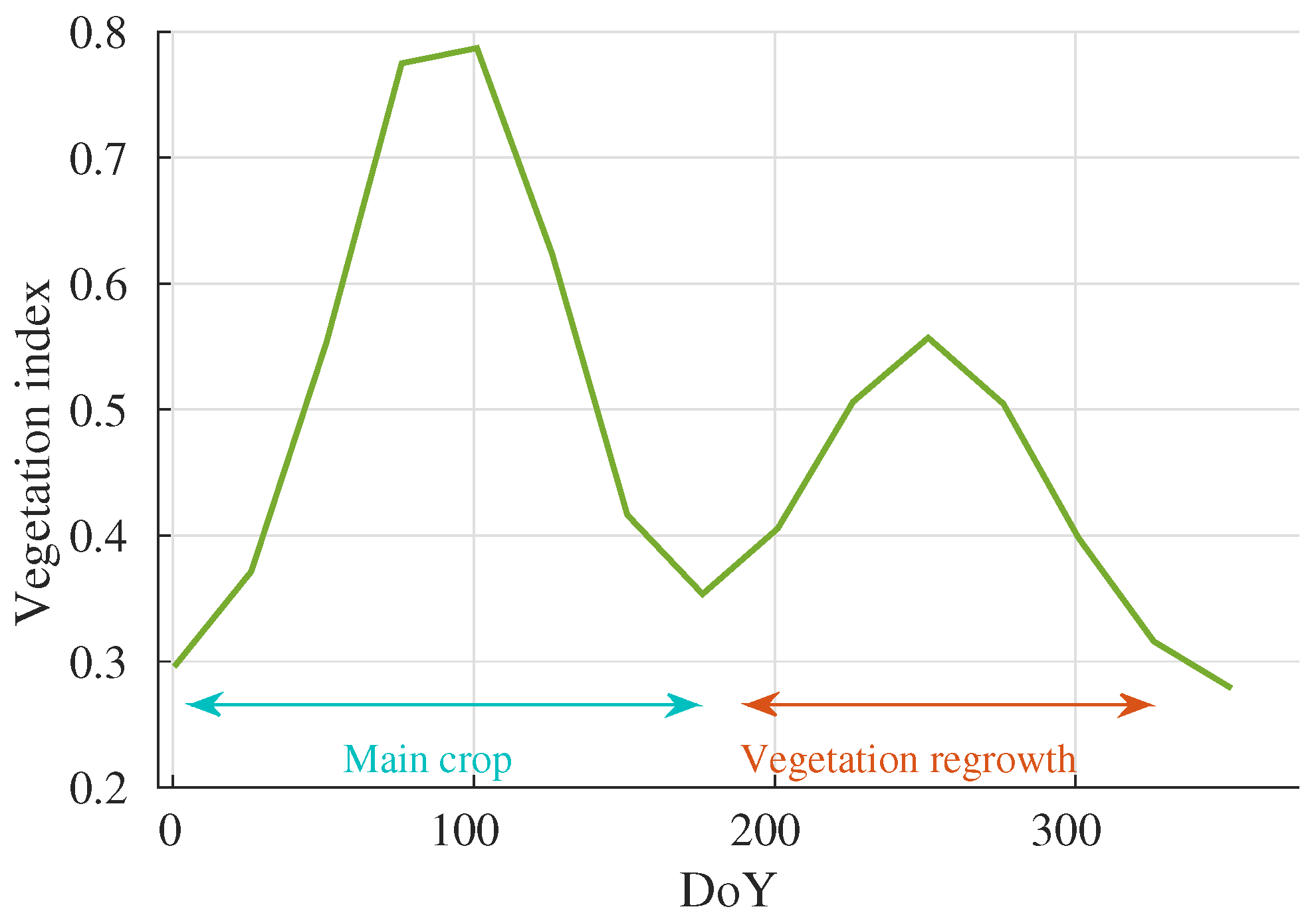
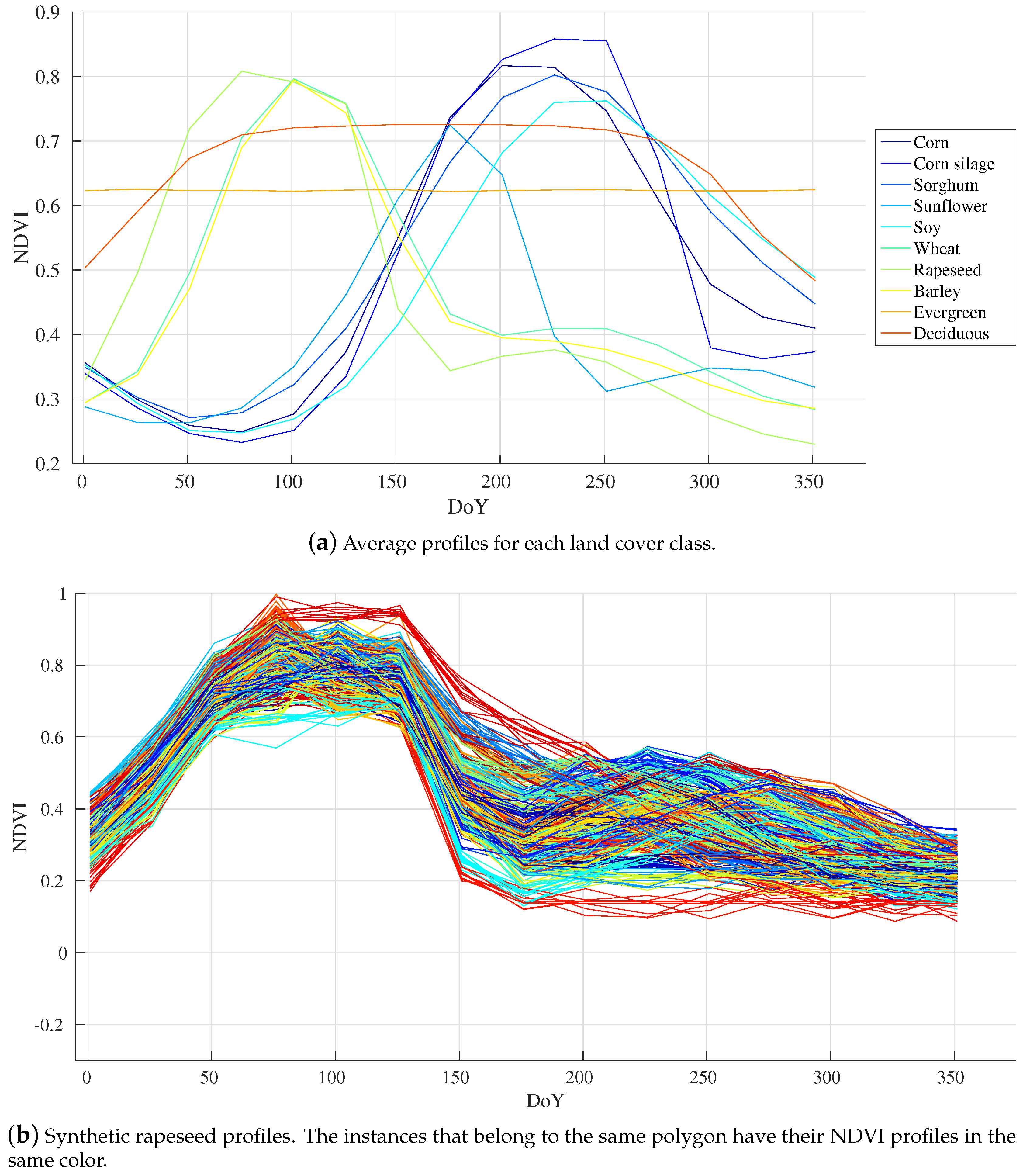
2.1.1. Synthetic Datasets

The creation of synthetic optical satellite image time series describing the heterogeneity of the landscapes and close to reality is not a straightforward task. Although some works exist to predict surface reflectance [43], it is almost impossible to create realistic models ensuring that the statistical properties of the synthetic products are close to those of remote sensing images.
However, some studies have shown that phenological vegetation characteristics can be modeled by using vegetation indexes, such as Normalized Difference Vegetation Index (NDVI). In the context of satellite image time series classification, NDVI has shown its ability to capture the vegetation growing [44], and its interest to detect phenology patterns [45]. For these reasons, the proposed synthetic datasets are based on the generation of synthetic NDVI profiles describing vegetation classes.
The remote sensing community has proposed several methods in order to fit NDVI profiles such as asymmetric Gaussian functions [46], piecewise logistic functions [47], or double logistic functions [48,49]. Following the model described in [50], a double logistic function defined with six parameters will be used:
N D V I ( t ) = A 1 1 + e x 0 t x 1 1 1 + e x 2 t x 3 + B ,
with A the amplitude, B the minimum value, x 0 and x 2 the inflection points, and x 1 (or x 3 ) the rate of increase (or decrease) of the curve at the inflection point. The fitting is only valid for the defined time period t. For vegetation classes such as croplands, t can represent one year. Furthermore, the double logistic function of Equation (1) can be only used to model the phenological cycle of one crop. The sum of several double logistic functions may simulate the development of several crops during the year, and also more complex classes.
In this study, it has been decided to use simulated NDVI profiles representing only one crop per year as feature vector. However, in order to create more realistic profiles, a vegetation regrowth has been simulated by adding a Gaussian function to the Equation (1). Vegetation regrowth appears after the phenological cycle described by Equation (1). Figure 1 displays an example of a main cycle followed by a vegetation regrowth. Finally, a uniform noise is added to Equation (1) in order to achieve a more realistic data variability.
The model described by Equation (1) is used to simulate the ten vegetation land cover classes that constitute the proposed synthetic dataset. There are five summer crops (corn, corn silage, sorghum, sunflower, and soy), three winter crops (wheat, rapeseed, and barley), and two forest classes (evergreen, and deciduous). Contrary to corn, the corn silage—used for animal feed—is harvested while still a bit green inducing a drastically drop during the crop senescence. Profiles have been simulated by using French expert’s knowledge, but the chosen land cover names are subjective and may not exactly characterize the produced synthetic profiles.
To bridge the gap between real and synthetic data, a polygon concept has been introduced to the simulation procedure. The idea is to take into account the field campaign protocols where instance labels are assigned by polygons describing for instance crop fields. Accordingly, each synthetic instance is defined by a feature vector, a land cover class, and a polygon identifier.
The simulation procedure mainly relies on the choice of two types of parameters: global parameters whose values are identical for all classes, and class parameters whose values depend on the land cover class to be simulated.
Three global parameters have been used: the date vector, t in Equation (1) expressed as Day of Year (DoY); n the number of instances per polygon; and n b p the number of polygons per land cover class. In balanced problems, multiplying the number of classes by n × n b p gives the total number of instances. For this study, t goes from 1 to 351 by a 25-step in DoY (15 dates, i.e., 15 features), n = 10 , and n b p = 100 .
For class parameters, an interval range from minimum ( m i n ) to maximum ( m a x ) values is defined for each of the parameters A, B, and x i ( 0 i < 4 ) from Equation (1). Table 1 displays the values for the ten land cover classes.
As mentioned above, each instance will have a polygon identifier. In remote sensing, instances coming from the same polygon have generally similar profiles. Thus, simulated instances from the same polygon should be more similar than other instances from the same class. Therefore, class parameter values are first randomly selected for polygon by using a normal distribution N ( μ , σ ) , with μ = m a x m i n 2 and σ = m a x μ 3 . 0 . Then, these polygon parameter values are used to define a polygon interval range, where polygon instance parameters are randomly selected. The same vegetation regrowth values—modeled by a Gaussian distribution—are assigned for all the polygon instances. Finally, these polygon instances are contaminated by a uniform noise.
Figure 2 shows some examples of simulated NDVI profiles as a function of DoY. More specifically, Figure 2a displays the land cover profiles obtained by averaging all profiles belonging to the same class. Figure 2b displays 500 rapeseed profiles. Rapeseed is a special case, which is simulated by the sum of two double logistic functions in order to reproduce rapeseed blooming. Each color represents profiles belonging to the same polygon. The vegetation regrowth simulation can be observed between DoY 175 and DoY 325.
Considering the simulation procedure, the three datasets described in Table 2 are generated. These datasets are composed of different number of land cover classes since this study aims at evaluating the influence of the number of classes on classification performances in the presence of class label noise. Besides, the 2-class dataset, composed of two similar classes, will allow to study rule-based noise influence.

2.1.2. Real Datasets

The studied real datasets have been obtained by extracting instance feature vectors from optical remote sensing images, and class label from real reference databases. Contrary to synthetic datasets, real datasets are not guaranteed label noise-free, but they better represent the land cover classification problem. In order to assess and validate results obtained on synthetic datasets, only vegetation classes have been studied in real datasets.
For this purpose, images coming from SPOT-4, Take-5 experiment [51], and Landsat-8 satellites have been used. The available images in 2013 are displayed in Figure 3 for both sensors. The use of SPOT-4 and Landsat-8 images allows to cover almost a complete year, and thus a complete vegetation cycle.
Landsat-8 images are spatially resampled at the 20 m spatial resolution of SPOT-4 images. Both sensor images are orthorectified and converted from digital number values to top-of-atmosphere reflectances by USGS (United States Geological Survey) or Theia Land Data Center. Then, the images are converted into top-of-canopy reflectance values by using the MACCS processing chain (Multi-sensor Atmospheric Correction and Cloud Screening) [52]. Cloudy data, identified by MACCS, are filled in with a temporal linear interpolation [11,53].
The French Land Parcel Information System database (Registre Parcellaire Graphique in French), has been used as reference database. This database annually maps French crop fields, which have been declared from the farmers. In this case, the used land cover classes correspond to two summer crops (sunflower and corn) and three winter crops (barley, wheat, and rapeseed). To limit the presence of class label noise coming from the database, two preprocessing tasks have been performed. First, polygons have been eroded of 80 m, then the smallest polygons have been deleted. The total number of extracted polygons per land cover class is given by Table 3.
In order to ensure that experimental configurations are comparable with those used for synthetic datasets, n b p polygons per land cover class are randomly selected in the reference database. Then, n instance feature vectors are randomly extracted for each selected polygon.
Similarly to synthetic datasets, vegetation land cover classes are firstly represented by NDVI profiles computed from satellite image time series. However, more features can be used as input data in the classification scheme. Taking benefit from SPOT-4 and Landsat-8 spectral resolutions, different datasets may be extracted to enhance classification performances. Accordingly, two other input spectral feature sets are studied: (1) spectral bands with NDVI (SB-NDVI); and (2) spectral bands with twelve spectral features including NDVI (SB-SF). Both input feature sets are described in [54]. Increasing the number of features also allows to study the influence of different input datasets in the presence of class label noise.
Table 4 presents the twelve configurations used for the experiments. As for the synthetic dataset, the total number of instances can be computed by multiplying the number of classes by n × n b p . Datasets 1 to 6 are composed of 1000 instances per land cover class, i.e., the same number of instances than for synthetic datasets. However, this number of instances is close to the feature vector sizes of SB-NDVI and SB-SF. In these cases, the learning process can be affected by the curse of dimensionality because the size of feature vectors is close or higher than the number of instances. To avoid this phenomenon, datasets 7 to 12 are studied. For these datasets, 40 instances are selected in 120 polygons for each land cover class, increasing the number of instances per class to 4800.

2.2. Noise Injection Procedure

To assess the classification results, a noise injection procedure generating artificial class label noise is required [28,31,32]. The knowledge of noisy instances allows to study the influence of class label noise [42], and also the effectiveness of mislabeled instance detection methods or cleansing filters [55,56].
Random and systematic class label noises are implemented for this study. Both procedures consist in injecting artificial class label noise to the datasets created in Section 2.1. It has been decided to generate class label noise for all the studied classes at several levels. Therefore, a x% noise level describes the percentage of instances affected by class label noise for each class. For example, a 5% noise level implies that all classes have 5% of their instances with wrong labels.
The random change considers that wrong label assignment is equiprobable between all the class labels except the original one. Thus, it prevents relabeling an instance with its original label contrary to [23,28]. This choice allows to have a current noise level equal to the theoretical one, which is independent of the number of classes. By contrast, the systematic label noise flips the label of corrupted instances belonging to the same class to an another class. In the case of binary classification, random and systematic label noise procedures are identical. Thus, the systematic label noise injection procedure is only applied on the 5-class datasets. Table 5 displays the corresponding flips applied for synthetic and real datasets. For the synthetic dataset, the noise class label has been selected randomly for each class. For the real dataset, the confusions have been introduced between the winter crops (wheat, barley and rapeseed) and between the summer crops (corn and sunflower).
The study of twenty noise levels ranging from 5% to 100% with 5% step is proposed. The noise will be generated for all the training datasets presented in Section 2.1. It has been decided that each noise level is independent. Specifically, if a given instance is corrupted at 5% noise level, it does not imply that the same instance will be corrupted at 10% noise level.
In the literature, the correlation between instances has not been taken into account during the noise generation. It means that traditional injection procedures operate at the instance level. Due to the specific nature of data coming from the remote sensing reference databases, this procedure can suffer from some limitations. Indeed, the reference database polygons are composed of correlated instances, i.e., with quite similar feature vectors, describing the same land cover class. In addition, the class label noise of real datasets generally affects whole polygon instances. For this reason, the used noise injection procedure corrupts all the polygon instances. On the other hand, if adding noise at polygon level results in a number of corrupted instances higher than the desired one, instances are randomly selected inside the polygon in order to respect the given noise level.

3. Classification Scheme

3.1. Classifier Algorithms

From several decades, land cover mapping system takes advantages from enhancements in machine learning. In this context, Support Vector Machines (SVM) are often baseline of studies due to their good classification performances. Ensemble methods (bootstrap, bagging, etc.) have also received great interest in the remote sensing community. In this category, several recent studies have highlighted the interest of Random Forests (RF) for land cover mapping [57,58,59].

3.1.1. Support Vector Machines

Support Vector Machines (SVM) have been widely used in the context of remote sensing classification [60,61,62]. SVM are based on the statistical learning theory proposed in [63,64].
Theoretically, SVM aim at finding the hyperplane that will optimally linearly separate two classes. For this purpose, SVM try to maximize the margin, i.e., the distance between the hyperplane and the closest instances to this hyperplane. The corresponding closest instances are named support vectors. The SVM classifier may be formulated as a quadratic optimization problem.
In order to define how flexible the classifier handles instances on the wrong side of the hyperplane, the soft-margin concept has been introduced [65]. It consists in accepting some misclassification errors when searching the best hyperplane. For this purpose, slack variables, that release the constraint on training data, are added in order to minimize the number of errors. The tradeoff between the importance of the slack variables and the margin is controlled by a regularization parameter C, also named penalty error.
As the data are not always linearly separable in the original dimension space, it has been proposed to embed the data in a higher dimension space where a linear separation can be found. The embedding consists in applying a non-linear transformation to the input data by using a kernel function, that allows to compute dot products in a higher dimensional space without explicitly transforming input data.
Different kernel functions have been proposed in the literature [66]. In this study, two kernel functions are analyzed: the linear and Radial Basis Function (RBF) kernels. For both kernels, the tuning of regularization parameter C is required. In addition, SVM-RBF kernel needs the optimization of a second parameter γ > 0 . This shape parameter controls the width of the Gaussian kernel function.
Working with multi-class problems, the classical “one-against-one” approach, implemented in LIBSVM [67], is used. Therefore, one SVM model is learned for each pair of classes. Finally, the prediction on new instances is done according to the maximum voting rule.

3.1.2. Random Forests

RF classifier consists in building K binary CART trees (Classification And Regression Trees [68]) [69]. The binary trees are learned on bootstrap instances, i.e., instances which are drawn with replacement from the training set [70].
At each node, a subset of m input features is randomly selected. Only the feature maximizing an impurity test, such as Gini coefficient or entropy, is used for splitting the node data.
The bootstrap procedure and the random feature subset selection may decrease the strength of individual trees. However, these operations reduce the correlation between the different trees, which decreases the generalization error.
For the prediction, new instances are classified by each RF tree. Finally, class labels are determined by using the maximum voting procedure.
To reduce training time without loosing accuracy, the tree growth can be interrupted when a maximum depth (denoted by m a x _ d e p t h ) is reached. Similarly, the split procedure can be stopped early when the number of instances in the node is under a m i n _ s a m p l e s threshold.

3.2. Sampling Strategy

The sampling procedure, applied to both synthetic and real datasets, aims at constructing two independent set of instances: one for the training and one for assessing the quality of the produced land cover map quality. The split is made at a polygon level (50% for training and 50% for testing) in order to ensure that there are no pixels from the same polygon in the training and the test sets. For each dataset, the procedure is repeated ten times in order not to influence the result by a specific split of reference data.
The ten independent training datasets are then corrupted by using the noise injection procedure described in Section 2.2. Finally, the evaluation is done at the pixel-level with the label noise-free test datasets obtained by the split procedure.

3.3. Evaluation

In order to evaluate the influence of class label noise with RF and SVM, the Overall Accuracy (OA) is calculated from confusion matrices obtained with label noise-free test sets. The obtained results are averaged over the ten runs for each noise level. The ten runs also allow the computation of the standard deviations for each classifier algorithm.
As described in Section 3.1, classifier performances depend on their required parameters. For SVM classifier, a logarithmic grid search approach is used in order to ensure the best parameter selection according to the training data. More precisely, the optimization is performed by using a five-fold cross-validation in two steps: one at a coarse resolution 2 5 , 2 4 , . . . , 2 4 , and the other one at a finer resolution v a l × 2 1 , v a l × 2 4 5 , v a l × 2 3 5 , . . . , v a l × 2 4 5 , with v a l the selected values at the coarse resolution. The optimization is performed for each training set, and may differ depending on the noise level. The C and γ parameters are optimized for the Gaussian kernel, whereas only C is optimized for the linear kernel. The input data are first standardized by subtracting the mean and dividing by the standard deviation. This assures that the distance measures to the hyperplane are not dominated by a single feature with an high dynamic range.
In the case of RF, parameters have a low influence on classification results [71,72,73]. They are set according to results presented in [54]: K = 200 , m = p with p the feature vector size, m a x _ d e p t h = 25 , and m i n _ s a m p l e s = 10 .

4. Results and Discussions

This section aims at evaluating the influence of training class label noise based on: (1) the noise level; and (2) the classifier choice. For this purpose, RF, SVM-Linear, and SVM-RBF classifiers have been tested on synthetic and real datasets.
Several classification configurations are studied in the following. Firstly, the impact of the number of classes, and the use of different input feature vectors and different number of training instances are tested with the injection of random label noise. Secondly, the algorithm complexity is studied for the random label noise. Then, the influence of systematic label noise is analyzed. Finally, the differences between the three classifiers are discussed.

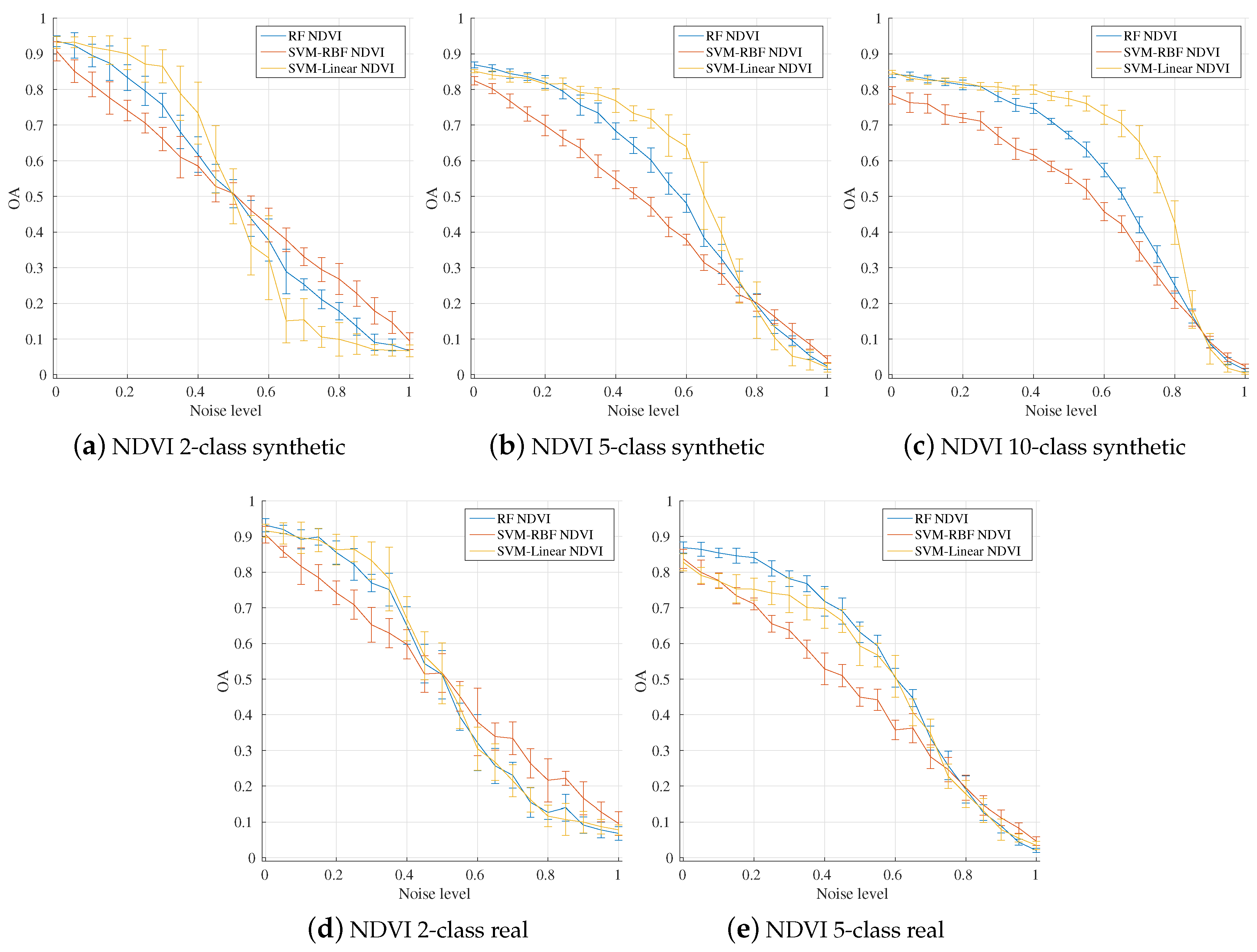
4.1. Influence of the Number of Classes

Firstly, random class label noise influence is evaluated through different number of classes on synthetic and real datasets. NDVI features are used as input data for the classification. For 2-class experiments, the random noise can be considered as rule-based noise since it is injected between similar land cover classes.
Figure 4 displays average OA over the ten runs as a function of the noise level. The first row shows the results for the three synthetic datasets (Table 2), whereas the second row shows the results for two real datasets (dataset number 1 and 4 from Table 4). Each curve color represents a different classifier: the blue for RF, the red for SVM-RBF, and the yellow for SVM-Linear. Error bars represent the standard deviation of classification accuracy over ten runs for each noise level.
Figure 4 illustrates how the three classifier performances decrease when the noise level increases. It shows that classifier performances remain stable for low noise levels, especially for SVM-Linear classifier. The 2-class experiments, Figure 4a,d, obtain the highest OA at 0% noise level. Despite both corn and corn silage classes having similar temporal behaviors, the good results are explained by the low classification complexity—only two classes to be classified. However, OA values of Figure 4a,d drop off more drastically than for 5- or 10-class datasets. For these binary problems, all mislabeled training instances are re-assigned to the other class; whereas for 5- or 10-class synthetic datasets, noise is randomly distributed among all the classes. Therefore, these results show that random class label noise is less harmful when the number of classes increases.
Comparing the results of the three classifiers, SVM-RBF obtains the lowest performances. Except for 10-class synthetic dataset, the SVM-RBF OA values decrease almost linearly with the noise level. On the other hand, Figure 4b–d show that RF and SVM-Linear classifiers have similar behaviors up to about 25% noise level. At these low noise levels, the emergence of flat zones corroborates the low influence of class label noise on both classifiers. For noise levels above of 25%, SVM-Linear is the most robust classifier except for the 5-class real dataset.
Figure 4 highlights the consistency of the created synthetic datasets. Indeed, the results on both rows of Figure 4 are very similar. However, RF classifier outperforms SVM-Linear for 5-class real dataset, which is not the case with synthetic dataset. In this real case, RF better deal with the land cover complexity than SVM-Linear.
To conclude these experiments, RF and SVM-Linear are more robust than SVM-RBF in the presence of random class label noise regardless the number of classes.

4.2. Influence of Input Feature Vectors

Classification performances in the presence of random label noise have been assessed in the previous section by only using NDVI feature vector as classifier input data. In real world applications, the use of more complex features may be considered with the availability of the new remote sensing data. Spectral bands and spectral features can be extracted for real datasets as described in Section 2.1. The goal here is therefore to compare the effect of random class label noise for different input feature vectors. More specifically, real datasets 1 to 6 of Table 4 are used. Accordingly, the 2-class and 5-class problems are analyzed.
Figure 5 displays average OA values as a function of the noise level for real datasets. The first row shows the results for 2-class problem, whereas the second row shows the results for 5-class problem. The first column displays results with NDVI, the second one with SB-NDVI, and the third one with SB-SF. Each curve color represents a different classifier: the blue for RF, the red for SVM-RBF, and the yellow for SVM-Linear.
For 2- and 5-class problems, SVM-Linear performances decrease linearly with SB-NDVI and SB-SF features (Figure 5b,c,e,f). These low performances are not observed with the use of only NDVI features (Figure 5a,d). By contrast, SVM-RBF performances decrease linearly with the use of NDVI features (Figure 5a,d); and higher OA values are observed with SB-NDVI or SB-SF features. Further analysis on classifiers will be discussed in Section 4.6.
Concerning RF classifier results, RF with SB-NDVI or SB-SF feature vectors outperform both SVM classifiers up to a 50% noise level. In addition, adding spectral features increases RF performances compared to the use of only NDVI features. In particular, this can be seen on the second row of Figure 5 for RF and SVM-RBF on 5-class real datasets. By contrast, no significant differences can be observed between SB-NDVI or SB-SF, which confirms the previous results obtained in [54].
To conclude, RF classifier is more robust than SVM in the presence of random class label noise when using spectral bands and spectral features.

4.3. Influence of the Number of Training Instances

Previous results show that adding spectral features may help for the improvement of classification performances. However, the high dimension of the previous problem can affect the classification performances. To evaluate this effect, the same input datasets and the same noise injection procedure as previously are used, but the number of training instances is here equal to 4800 (or 12,000) for 2- (or 5-) class problem (dataset number 7 to 12 from Table 4).
Following the same figure style than previously, Figure 6 shows classification performances for different noise levels. The first row displays the results for 2-class problem with 4800 training instances, whereas the second row displays the results for 5-class problem with 12,000 training instances. From left to right, NDVI, SB-NDVI, and SB-SF input feature vectors are used. Each curve color represents a different classifier: the blue for RF, the red for SVM-RBF, and the yellow for SVM-Linear. Thus, Figure 5 and Figure 6 display the results on the same datasets composed of 500 and 2400 training instances per class respectively.
Adding instances does not significantly affect the results. For all the configurations—classifier, features, number of classes—trends are the same as those with fewer instances. However, the RF performances slightly decrease, and the SVM performances slightly increase.

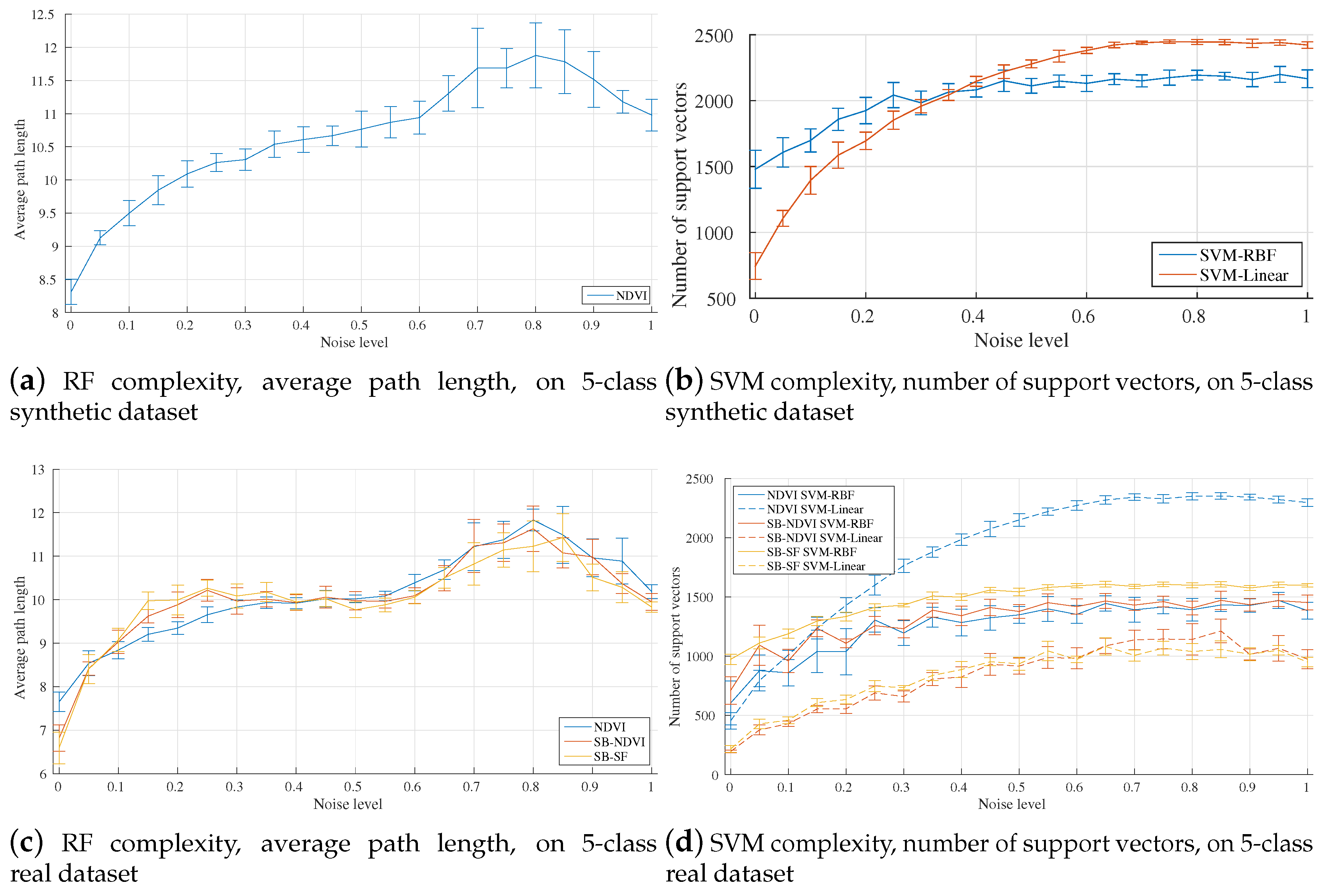
4.4. Algorithm Complexity

Algorithm complexity has also been studied in order to examine the impact of class label noise on algorithm behaviors. In the case of RF, the complexity is evaluated by computing the average path length of each training instance. A small average path length means a simple model to learn and a rapid decision phase. Concerning the SVM algorithm, the number of support vectors has been selected to represent the SVM complexity. The number of support vectors depends on the distribution of the data and the value of the C parameter. A small number of support vectors corresponds to a simple model to learn.
These experiments have been carried out by using 2500 training instances for 5-class synthetic and real datasets with random label noise. NDVI, SB-NDVI, and SB-SF have been used (dataset number 4 to 6 from Table 4).
Figure 7 displays RF and SVM complexities as a function of noise level. The first row shows the complexity for the synthetic dataset, whereas the second row shows the complexity for the real dataset. In the case of real dataset, each curve color represents an input feature vectors: blue for NDVI, red for SB-NDVI, and yellow for SB-SF. Figure 7a,c display the average path length averaged for each tree of the RF classifier. Figure 7b,d display the number of support vectors for SVM algorithm. In Figure 7d, solid lines represent obtained results for SVM-RBF classifier, whereas dashed lines correspond to SVM-Linear results
As expected, the complexity of algorithms increases with the noise level. Accordingly, the presence of noise will also impact training requirements such as computational time and memory need.
For RF, the model complexity is similar for the different input feature datasets. However, the SB-SF and SB-NDVI complexities are lower than NDVI complexity at a 0% noise level. By using more features, the quality of feature subsets selected at each node is improved. Thus, the split quality is also enhanced, leading to a reduction in the required number of splits. Figure 7a,c show that the RF complexity curves follow three stages. During the first stage, Figure 4b,e shows a slight decrease of the OA values. At these low noise levels, the RF classifier manages the mislabeled data resulted in an increase of RF complexity. Then, the RF complexity remains stable when the OA values fall steadily. In this case, the RF classifier assimilates mislabeled data as normal data. After 50% noise level, the RF complexity increases again due to the excessive presence of mislabeled training data. In addition, the average path length for the synthetic dataset is higher than for real datasets due to the size of the input feature vectors, which is smaller for the synthetic dataset. A higher average path length involves a slower decision phase for new instances. However, the training computational time, which is much higher than decision phase time, increases with the number of features.
Considering SVM-RBF complexity, the addition of more features requires the use of more support vectors. The Gaussian kernel embeds data in a higher dimension space, leading to the possibility to select more support vectors. Thus, it may explain why the number of selected support vectors is higher for SVM-RBF than for SVM-Linear. However, NDVI SVM-Linear is an exception, since the number of support vectors is higher than NDVI SVM-RBF for high noise levels.

4.5. Study of Systematic Label Noise

Previous studies have been performed for the generation of a random label noise. To analyze the effect of more realistic mislabeled data, the study of systematic label noise is performed for the 5-class synthetic and real datasets with NDVI features.
Figure 8 displays average OA values over the ten runs as a function of the noise level. Figure 8a shows the results for 5-class synthetic dataset, whereas Figure 8b shows the results for 5-class real dataset. Each curve color represents a different classifier: the blue for RF, the red for SVM-RBF, and the yellow for SVM-Linear.
The results show that the systematic label noise is similar to the random label noise, but more harmful (Figure 4b,e). Thus, a short plateau can be observed at low noise levels for the RF and SVM-Linear classifiers. In addition, the OA values decrease more strongly. For instance, at 40% noise level, the RF OA values of the 5-class real dataset are equal to 72% and 60% for random and systematic noise respectively. As for the random label noise, the SVM-RBF OA values decrease linearly with the noise level. The SVM-RBF classifier is the most impacted classifier by the systematic label noise.
The systematic label noise has an higher influence on the classification performances than the random label noise. In addition, the RF classifier is more robust to the systematic label noise than the SVM-RBF and the SVM-Linear classifiers.

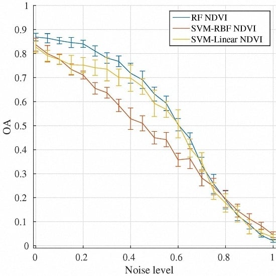
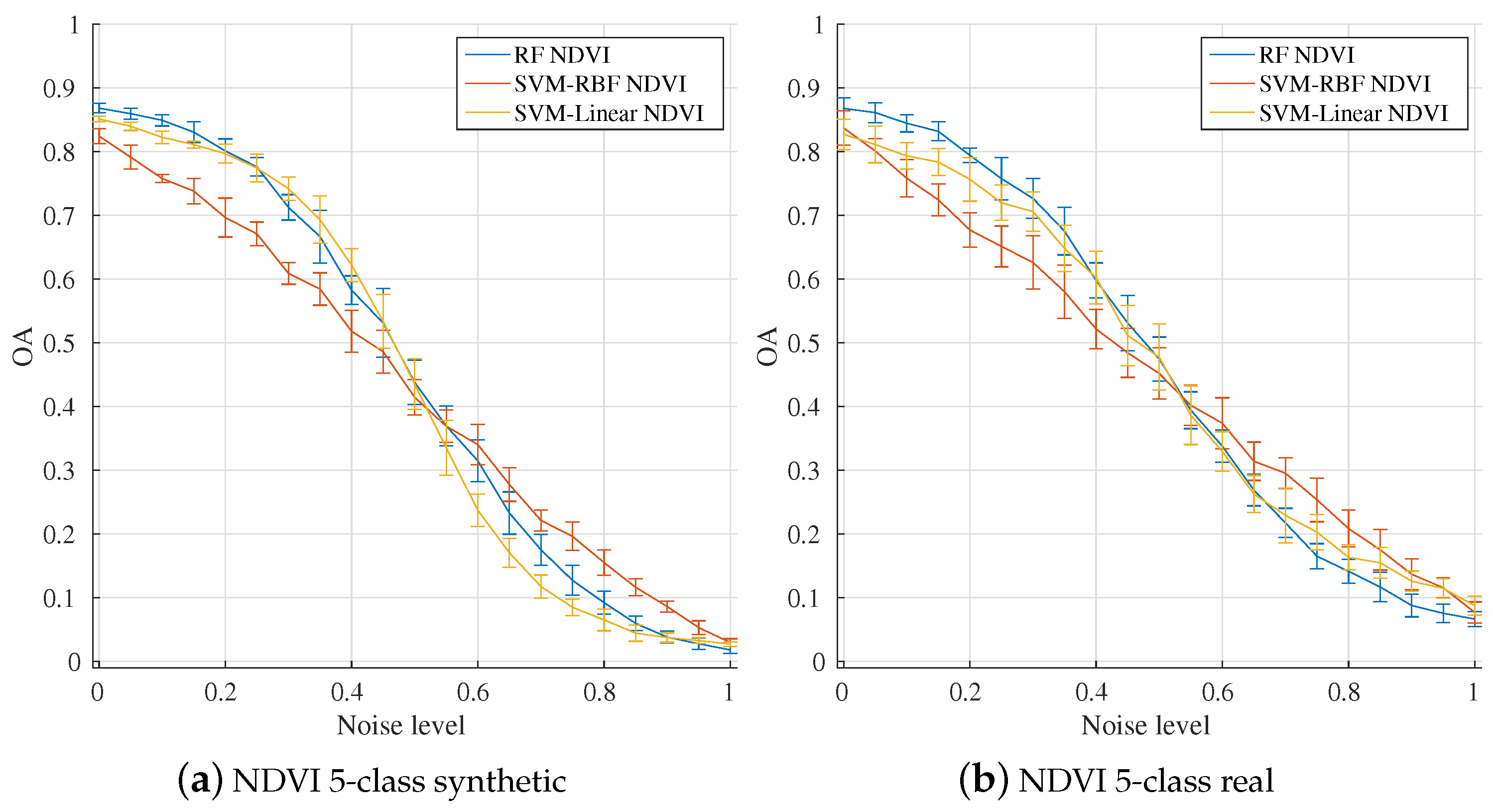
4.6. Comparison between Classifiers

The results obtained in the previous sections show how the performances decrease with the presence of class label noise. Comparing all classifier results, RF seem less sensitive to noise than SVM. Furthermore, RF have similar behaviors for the studied configurations: changing the number of classes, increasing the number of instances, or adding some features to the input vector.
This result complies with the literature. In [37], eleven classifiers, including RF and SVM-Linear, are compared on different datasets. The RF classifier is the most robust among the eleven. Similarly, RF yield better performances than SVM-RBF in [74]. However, the classifier parameters were not optimized in this study, that may be more adverse for SVM-RBF. The effect of noise in the training set has also been studied in [14]: the RF classifier was more robust than a single classification tree.
The RF robustness to class label noise can be related to its good generalization ability. It relies on the construction of several decorrelated trees due to bootstrap operation, but also to a sufficient number of trees and the split procedure, i.e., each node building with only one feature selected from a subset. Therefore, it is usual to assume that RF, with a careful parameter setting [75], are less likely to overfit than some other methods.
SVM classifiers with two different kernels seem to have complementary behaviors. SVM-Linear classifier is more robust to noise presence with a small feature vector size, whereas SVM-RBF is more robust to the presence of noise with a large feature vector size.
In the case of a small feature set, the poor SVM-RBF performances may be due to overfitting. The embedding in a space of higher dimension allows SVM-RBF to find an optimal hyperplane that perfectly follows training instances. The γ parameter sets the width of RBF kernel. When the γ value is small, the model is too constrained and cannot capture the data structure. The resulting model behaves similarly to a linear classifier. By contrast, a model learned with a large γ value is very sensitive to the input data, i.e., it tries harder to avoid misclassifying in the training dataset. Thus, the model looses its learning generalization ability, and has difficulty to classify new instances.
The γ values obtained for SVM-RBF classifier are studied to validate the SVM behavior. Table 6 displays γ values selected with cross-validation for 5-class 2500-instance real dataset for the three input feature sets. The poor performances of SVM-RBF with NDVI features shown in Figure 5d, correspond to high γ values (>0.1), displayed on the first row of Table 6. In this case, the low accuracy results indicate the overfitting of the SVM-RBF classifier. On the contrary, Figure 5e,f, that display good OA values for small noise levels, correspond to small γ values. In the case of NDVI features, the feature space is too small, and the model cannot adequately capture the variability of the data. Thus, the cross-validation procedure, used to select the optimal parameter values, seems to lead to overfitting in the case of small feature space [76].
To validate the previous hypothesis, the cross-validation performances are evaluated in the presence of random class label noise. For SVM-RBF classifier, all the C - γ configurations of the coarse grid search described in Section 3.3 are tested on training and test sets. The experiments are carried out for the 5-class real dataset with NDVI features and 2500 training instances. The purpose is to compare the optimal parameter values obtained by the cross-correlation on training set to the optimal one expected for the testing data.
Figure 9 displays the cross-validation performances for SVM-RBF classifier at 0%, 20%, 40% noise levels. For each figure, the horizontal and vertical axis display C and γ values respectively in logarithmic scale. The first row shows OA obtained by the five-fold cross-validation procedure on the training set. By contrast, the second row shows OA obtained on an independent test set. The red cross highlights the selected parameter values found with the five-cross validation procedure, i.e., the highest OA obtained with the training set.
Figure 9a–c shows that the optimal values found by cross-validation procedure (red crosses) remain similar for the three noise levels. This optimal parameter values correspond to the best average OA computed over test folds that also contain mislabeled instances. The best C values seem limited for the three noise levels; higher C values have been tested giving similar results.
Figure 9d–f show that optimal values, i.e., high OA values, change when the noise level increases. For the three studied noise levels, optimal γ and C values obtained with independent test set are smaller than optimal values selected by the cross-validation procedure. In this case, SVM-RBF overfits.
In contrary, SVM-Linear is more robust to noise with only NDVI features. Figure 4e shows that SVM-Linear is less prone to overfitting than SVM-RBF with NDVI features. Due to the small size of the feature space, SVM-Linear does not have a large number of choices to construct its linear decision. Therefore, the C parameter optimization has a low influence on the results. By contrast, SVM-Linear classifier has many possibilities with high feature space (Figure 5e,f), leading to overfitting.
Hence, these results show that SVM classifier can be very sensitive to its parameter configuration. Furthermore, the above results show that the cross-validation procedure may be impacted by the presence of noise.

5. Conclusions

The effect of mislabeled training data on supervised classification has been analyzed and discussed in this work. Specifically, the robustness of three supervised methods in the presence of training class label noise is evaluated. To the authors’ knowledge, the effect of such noise has not been yet analyzed for land cover mapping with satellite image time series.
The three well known classifiers RF, SVM-RBF and SVM-Linear, have been compared with different noise levels and different classification configurations. For this purpose, experiments have been carried out on synthetic and real datasets. The synthetic dataset has been specifically designed for this study. It simulates vegetation profiles over one year. A new strategy to inject class label noise based on polygons has also been proposed.
The general results have shown that RF and SVM are robust classifiers for low noise levels in the presence of mislabeled training data. The impact of training random class label noise has also been studied through different classification configurations. Firstly, the influence of the number of classes has been analyzed. The 2-class datasets imply difficult problems, where accuracies decrease faster than 5- or 10-class problems. These experiments have also corroborated the consistency of the synthetic dataset, where the same trends have been observed on real datasets. However, they have been carried out only with NDVI features as input data, showing some overfitting for SVM-RBF. Therefore, a second experiment has been performed by adding more features as input data to the classification system. The addition of spectral features to NDVI generally improves classification performances. Contrary to the first experiment, the SVM-RBF classifier outperforms SVM-Linear by avoiding overfitting. Furthermore, the algorithm complexities have also been studied, highlighting the importance of a good training set quality in order to reduce computational time and required used memory. As expected, the complexity of algorithms increases when noise level increases. Then, it has been observed that systematic label noise has a worse impact than random label noise on the classification performances. Finally, the classifier behaviors have been analyzed. RF algorithm is more robust to low class label noise levels in most of experiment configurations thanks to the bootstrap operation and the random split construction. The parametrization of SVM was not straightforward. More specifically, it has been shown that the cross-validation procedure is impacted by the noise presence, leading to classifier overfitting.
An interesting future work may focus on realistic land cover confusions. This harmful noise would probably have more impact on both SVM and RF classifiers. Similarly, only balanced problems have been analyzed here. However, in real classification problems, there are major and minor land cover classes representing the landscapes. Therefore, the influence of noise on imbalanced datasets could also be studied in the future.
Furthermore, this work focuses only on mislabeled training instances, but validation instances may also be noisy. It could be therefore interesting to characterize the classification performances as a function of validation class label noise to assess the procedure used to validate map accuracies [17,22].

Acknowledgments

This work is funded by the French spatial agency (CNES) and the French mapping agency (IGN), and it has been carried out at CESBIO laboratory—supported by the University Paul Sabatier, CNRS (Centre National de la Recherche Scientifique), CNES, IRD (Institut de Recherche pour le Développement)—and MATIS laboratory supported by IGN. The SPOT-4 imagery was obtained under the SPOT-4/Take-5 program. The SPOT-4/Take-5 imagery is copyrighted to CNES under “CNES 2013, all rights reserved. Commercial use of the product prohibited”.

Author Contributions

Charlotte Pelletier and Silvia Valero are the main authors of this manuscript. Charlotte Pelletier, Silvia Valero, Jordi Inglada, Nicolas Champion and Claire Marais Sicre designed and implemented the processing chain and processed the data. Gérard Dedieu participated in discussions during the system design and evaluation. He gave valuable methodological advice. All authors have been involved in the writing of the manuscript.

Conflicts of Interest

The authors declare no conflict of interest.

Abbreviations

The following abbreviations are used in this manuscript:
RFRandom Forests
SVMSupport Vector Machines
RBFRadial Basis Function
USGSUnited States Geological Survey
MACCSMulti-sensor Atmospheric Correction and Cloud Screening
NDVINormalized Difference Vegetation Index
SBSpectral Bands
SFSpectral Features

References

  1. Alcantara, C.; Kuemmerle, T.; Prishchepov, A.V.; Radeloff, V.C. Mapping abandoned agriculture with multi-temporal MODIS satellite data. Remote Sens. Environ. 2012, 124, 334–347. [Google Scholar] [CrossRef]
  2. Qamer, F.M.; Shehzad, K.; Abbas, S.; Murthy, M.; Xi, C.; Gilani, H.; Bajracharya, B. Mapping deforestation and forest degradation patterns in western Himalaya, Pakistan. Remote Sens. 2016, 8, 385. [Google Scholar] [CrossRef]
  3. Lefebvre, A.; Sannier, C.; Corpetti, T. Monitoring urban areas with Sentinel-2A data: Application to the update of the Copernicus high resolution layer imperviousness degree. Remote Sens. 2016, 8, 606. [Google Scholar] [CrossRef]
  4. Friedl, M.A.; Brodley, C.E. Decision tree classification of land cover from remotely sensed data. Remote Sens. Environ. 1997, 61, 399–409. [Google Scholar] [CrossRef]
  5. Waske, B.; Braun, M. Classifier ensembles for land cover mapping using multitemporal SAR imagery. ISPRS J. Photogramm. Remote Sens. 2009, 64, 450–457. [Google Scholar] [CrossRef]
  6. Li, M.; Zang, S.; Zhang, B.; Li, S.; Wu, C. A review of remote sensing image classification techniques: The role of spatio-contextual information. Eur. J. Remote Sens. 2014, 47, 389–411. [Google Scholar] [CrossRef]
  7. Szuster, B.W.; Chen, Q.; Borger, M. A comparison of classification techniques to support land cover and land use analysis in tropical coastal zones. Appl. Geogr. 2011, 31, 525–532. [Google Scholar] [CrossRef]
  8. Khatami, R.; Mountrakis, G.; Stehman, S.V. A meta-analysis of remote sensing research on supervised pixel-based land-cover image classification processes: General guidelines for practitioners and future research. Remote Sens. Environ. 2016, 177, 89–100. [Google Scholar] [CrossRef]
  9. Gómez, C.; White, J.C.; Wulder, M.A. Optical remotely sensed time series data for land cover classification: A review. ISPRS J. Photogramm. Remote Sens. 2016, 116, 55–72. [Google Scholar] [CrossRef]
  10. Sharma, R.C.; Tateishi, R.; Hara, K.; Iizuka, K. Production of the Japan 30-m land cover map of 2013–2015 using a Random Forests-based feature optimization approach. Remote Sens. 2016, 8, 429. [Google Scholar] [CrossRef]
  11. Inglada, J.; Arias, M.; Tardy, B.; Hagolle, O.; Valero, S.; Morin, D.; Dedieu, G.; Sepulcre, G.; Bontemps, S.; Defourny, P.; et al. Assessment of an operational system for crop type map production using high temporal and spatial resolution satellite optical imagery. Remote Sens. 2015, 7, 12356–12379. [Google Scholar] [CrossRef]
  12. Belgiu, M.; Drăguţ, L. Random Forest in remote sensing: A review of applications and future directions. ISPRS J. Photogramm. Remote Sens. 2016, 114, 24–31. [Google Scholar] [CrossRef]
  13. Tatsumi, K.; Yamashiki, Y.; Torres, M.A.C.; Taipe, C.L.R. Crop classification of upland fields using Random forest of time-series Landsat 7 ETM+ data. Comput. Electron. Agric. 2015, 115, 171–179. [Google Scholar] [CrossRef]
  14. Rodriguez-Galiano, V.; Ghimire, B.; Rogan, J.; Chica-Olmo, M.; Rigol-Sanchez, J. An assessment of the effectiveness of a Random Forest classifier for land-cover classification. ISPRS J. Photogramm. Remote Sens. 2012, 67, 93–104. [Google Scholar] [CrossRef]
  15. Pal, M. Random Forest classifier for remote sensing classification. Int. J. Remote Sens. 2005, 26, 217–222. [Google Scholar] [CrossRef]
  16. Meyer, H.; Kühnlein, M.; Appelhans, T.; Nauss, T. Comparison of four machine learning algorithms for their applicability in satellite-based optical rainfall retrievals. Atmos. Res. 2016, 169, 424–433. [Google Scholar] [CrossRef]
  17. Congalton, R.G.; Green, K. Assessing the Accuracy of Remotely Sensed Data: Principles and Practices; CRC Press: Boca Raton, FL, USA, 2008. [Google Scholar]
  18. Demir, B.; Persello, C.; Bruzzone, L. Batch-Mode active-learning methods for the interactive classification of remote sensing images. IEEE Trans. Geosci. Remote Sens. 2011, 49, 1014–1031. [Google Scholar] [CrossRef]
  19. Tuia, D.; Volpi, M.; Copa, L.; Kanevski, M.; Munoz-Mari, J. A survey of active learning algorithms for supervised remote sensing image classification. IEEE J. Sel. Top. Signal Process. 2011, 5, 606–617. [Google Scholar] [CrossRef]
  20. Radoux, J.; Lamarche, C.; Van Bogaert, E.; Bontemps, S.; Brockmann, C.; Defourny, P. Automated training sample extraction for global land cover mapping. Remote Sens. 2014, 6, 3965. [Google Scholar] [CrossRef]
  21. Fritz, S.; McCallum, I.; Schill, C.; Perger, C.; Grillmayer, R.; Achard, F.; Kraxner, F.; Obersteiner, M. Geo-Wiki.Org: The use of crowdsourcing to improve global land cover. Remote Sens. 2009, 1, 345–354. [Google Scholar] [CrossRef]
  22. Foody, G.M. Status of land cover classification accuracy assessment. Remote Sens. Environ. 2002, 80, 185–201. [Google Scholar] [CrossRef]
  23. Zhu, X.; Wu, X. Class noise vs. attribute noise: A quantitative study. Artif. Intell. Rev. 2004, 22, 177–210. [Google Scholar] [CrossRef]
  24. Nettleton, D.F.; Orriols-Puig, A.; Fornells, A. A study of the effect of different types of noise on the precision of supervised learning techniques. Artif. Intell. Rev. 2010, 33, 275–306. [Google Scholar] [CrossRef]
  25. Frénay, B.; Verleysen, M. Classification in the presence of label noise: A survey. IEEE Trans. Neural Netw. Learn. Syst. 2014, 25, 845–869. [Google Scholar] [CrossRef] [PubMed]
  26. Zhu, X.; Wu, X.; Chen, Q. Eliminating class noise in large datasets. In Proceedings of the Twentieth International Conference on Machine Learning (ICML), Washington, DC, USA, 21–24 August 2003; pp. 920–927.
  27. Xiao, T.; Xia, T.; Yang, Y.; Huang, C.; Wang, X. Learning from massive noisy labeled data for image classification. In Proceedings of the IEEE Conference on Computer Vision and Pattern Recognition, Boston, MA, USA, 7–12 June 2015; pp. 2691–2699.
  28. Teng, C.M. Correcting noisy data. In Proceedings of the International Conference on Machine Learning, Bled, Slovenia, 27–30 June 1999; pp. 239–248.
  29. Rebbapragada, U.; Brodley, C.E. Class noise mitigation through instance weighting. In Proceedings of the European Conference on Machine Learning, Warsaw, Poland, 17–21 September 2007; pp. 708–715.
  30. Brodley, C.E.; Friedl, M.A. Identifying and eliminating mislabeled training instances. In Proceedings of the American Association for Artificial Intelligence (AAAI)/Innovative Applications of Artificial Intelligence (IAAI), Portland, OR, USA, 04–08 August 1996; American Association for Artificial Intelligence: Menlo Park, CA, USA, 1996; pp. 799–805. [Google Scholar]
  31. Brodley, C.E.; Friedl, M.A. Identifying mislabeled training data. J. Artif. Intell. Res. 1999, 11, 131–167. [Google Scholar]
  32. Mellor, A.; Boukir, S.; Haywood, A.; Jones, S. Exploring issues of training data imbalance and mislabelling on Random Forest performance for large area land cover classification using the ensemble margin. ISPRS J. Photogramm. Remote Sens. 2015, 105, 155–168. [Google Scholar] [CrossRef]
  33. Xiao, H.; Xiao, H.; Eckert, C. Adversarial Label Flips Attack on Support Vector Machines. In Proceedings of the Twentieth European Conference on Artificial Intelligence (ECAI), Montpellier, France, 27–31 August 2012; pp. 870–875.
  34. Biggio, B.; Nelson, B.; Laskov, P. Support Vector Machines under adversarial label noise. ACML 2011, 20, 97–112. [Google Scholar]
  35. Görnitz, N.; Porbadnigk, A.; Binder, A.; Sannelli, C.; Braun, M.L.; Müller, K.R.; Kloft, M. Learning and Evaluation in Presence of Non-IID Label Noise. In Proceedings of the International Conference on Artificial Intelligence and Statistics, Reykjavik, Iceland, 22–25 April 2014; pp. 293–302.
  36. Teng, C.M. A Comparison of Noise Handling Techniques. In Proceedings of the International Florida Artificial Intelligence Research Society Conference, Key West, FL, USA, 21–23 May 2001; pp. 269–273.
  37. Folleco, A.; Khoshgoftaar, T.M.; Hulse, J.V.; Napolitano, A. Identifying Learners Robust to Low Quality Data. Informatica 2009, 33, 245–259. [Google Scholar]
  38. Garcia, L.P.; de Carvalho, A.C.; Lorena, A.C. Effect of label noise in the complexity of classification problems. Neurocomputing 2015, 160, 108–119. [Google Scholar] [CrossRef]
  39. Pechenizkiy, M.; Tsymbal, A.; Puuronen, S.; Pechenizkiy, O. Class noise and supervised learning in medical domains: The effect of feature extraction. In Proceedings of the 19th IEEE Symposium on Computer-Based Medical Systems (CBMS’06), Salt Lake City, UT, USA, 22–23 June 2006; pp. 708–713.
  40. Carlotto, M.J. Effect of errors in ground truth on classification accuracy. Int. J. Remote Sens. 2009, 30, 4831–4849. [Google Scholar] [CrossRef]
  41. Natarajan, N.; Dhillon, I.S.; Ravikumar, P.K.; Tewari, A. Learning with Noisy Labels. In Advances in Neural Information Processing Systems 26; Curran Associates, Inc.: Lake Tahoe, USA, 2013; pp. 1196–1204. [Google Scholar]
  42. Xiao, H.; Biggio, B.; Nelson, B.; Xiao, H.; Eckert, C.; Roli, F. Support Vector Machines under adversarial label contamination. Neurocomputing 2015, 160, 53–62. [Google Scholar] [CrossRef]
  43. Gao, F.; Masek, J.; Schwaller, M.; Hall, F. On the blending of the Landsat and MODIS surface reflectance: Predicting daily Landsat surface reflectance. IEEE Trans. Geosci. Remote Sens. 2006, 44, 2207–2218. [Google Scholar]
  44. DeFries, R.; Townshend, J. NDVI-derived land cover classifications at a global scale. Int. J. Remote Sens. 1994, 15, 3567–3586. [Google Scholar] [CrossRef]
  45. Senf, C.; Leitão, P.J.; Pflugmacher, D.; van der Linden, S.; Hostert, P. Mapping land cover in complex Mediterranean landscapes using Landsat: Improved classification accuracies from integrating multi-seasonal and synthetic imagery. Remote Sens. Environ. 2015, 156, 527–536. [Google Scholar] [CrossRef]
  46. Jönsson, P.; Eklundh, L. TIMESAT—A program for analyzing time-series of satellite sensor data. Comput. Geosci. 2004, 30, 833–845. [Google Scholar] [CrossRef]
  47. Zhang, X.; Friedl, M.A.; Schaaf, C.B.; Strahler, A.H.; Hodges, J.C.; Gao, F.; Reed, B.C.; Huete, A. Monitoring vegetation phenology using MODIS. Remote Sens. Environ. 2003, 84, 471–475. [Google Scholar] [CrossRef]
  48. Fisher, J.I.; Mustard, J.F.; Vadeboncoeur, M.A. Green leaf phenology at Landsat resolution: Scaling from the field to the satellite. Remote Sens. Environ. 2006, 100, 265–279. [Google Scholar] [CrossRef]
  49. Beck, P.S.; Atzberger, C.; Høgda, K.A.; Johansen, B.; Skidmore, A.K. Improved monitoring of vegetation dynamics at very high latitudes: A new method using MODIS NDVI. Remote Sens. Environ. 2006, 100, 321–334. [Google Scholar] [CrossRef]
  50. Inglada, J. PhenOTB, Phenological Analysis for Image Time Series. 2016. Available online: http://tully.ups-tlse.fr/jordi/phenotb (assessed on 16 February 2017).
  51. Hagolle, O.; Sylvander, S.; Huc, M.; Claverie, M.; Clesse, D.; Dechoz, C.; Lonjou, V.; Poulain, V. SPOT-4 (Take 5): Simulation of Sentinel-2 time series on 45 large sites. Remote Sens. 2015, 7, 12242–12264. [Google Scholar] [CrossRef]
  52. Hagolle, O.; Huc, M.; Villa Pascual, D.; Dedieu, G. A multi-temporal and multi-spectral method to estimate aerosol optical thickness over land, for the atmospheric correction of FormoSat-2, LandSat, VENμS and Sentinel-2 images. Remote Sens. 2015, 7, 2668. [Google Scholar] [CrossRef]
  53. Inglada, J. OTB Gapfilling, A Temporal Gapfilling for Image Time Series Library. 2016. Available online: http://tully.ups-tlse.fr/jordi/temporalgapfilling (assessed on 16 February 2017).
  54. Pelletier, C.; Valero, S.; Inglada, J.; Champion, N.; Dedieu, G. Assessing the robustness of Random Forests to map land cover with high resolution satellite image time series over large areas. Remote Sens. Environ. 2016, 187, 156–168. [Google Scholar] [CrossRef]
  55. Smith, M.R.; Martinez, T. Improving classification accuracy by identifying and removing instances that should be misclassified. In Proceedings of the 2011 International Joint Conference on Neural Networks (IJCNN), San Jose, CA, USA, 31 July–5 August 2011; pp. 2690–2697.
  56. Feng, W.; Boukir, S.; Guo, L. Identification and correction of mislabeled training data for land cover classification based on ensemble margin. In Proceedings of the IEEE International Geoscience and Remote Sensing Symposium 2015 (IGARSS), Milan, Italy, 26–31 July 2015; pp. 4991–4994.
  57. Hüttich, C.; Gessner, U.; Herold, M.; Strohbach, B.J.; Schmidt, M.; Keil, M.; Dech, S. On the suitability of MODIS time series metrics to map vegetation types in dry savanna ecosystems: A case study in the Kalahari of NE Namibia. Remote Sens. 2009, 1, 620–643. [Google Scholar] [CrossRef]
  58. Corcoran, J.M.; Knight, J.F.; Gallant, A.L. Influence of multi-source and multi-temporal remotely sensed and ancillary data on the accuracy of Random Forest classification of wetlands in Northern Minnesota. Remote Sens. 2013, 5, 3212–3238. [Google Scholar] [CrossRef]
  59. Immitzer, M.; Vuolo, F.; Atzberger, C. First experience with Sentinel-2 data for crop and tree species classifications in Central Europe. Remote Sens. 2016, 8, 166. [Google Scholar] [CrossRef]
  60. Huang, C.; Davis, L.S.; Townshend, J. An assessment of Support Vector Machines for land cover classification. Int. J. Remote Sens. 2002, 23, 725–749. [Google Scholar] [CrossRef]
  61. Jia, K.; Liang, S.; Wei, X.; Yao, Y.; Su, Y.; Jiang, B.; Wang, X. Land cover classification of Landsat data with phenological features extracted from time series MODIS NDVI data. Remote Sens. 2014, 6, 11518–11532. [Google Scholar] [CrossRef]
  62. Dusseux, P.; Corpetti, T.; Hubert-Moy, L.; Corgne, S. Combined use of multi-temporal optical and radar satellite images for grassland monitoring. Remote Sens. 2014, 6, 6163–6182. [Google Scholar] [CrossRef]
  63. Vapnik, V.N. The Nature of Statistical Learning Theory; Springer-Verlag: New York, NY, USA, 1995. [Google Scholar]
  64. Vapnik, V.N. Statistical Learning Theory; Wiley: New York, NY, USA, 1998. [Google Scholar]
  65. Cortes, C.; Vapnik, V. Support-Vector Networks. Mach. Learn. 1995, 20, 273–297. [Google Scholar] [CrossRef]
  66. Schölkopf, B.; Smola, A.J. Learning with Kernels: Support Vector Machines, Regularization, Optimization, and Beyond; MIT Press: London, UK, 2002. [Google Scholar]
  67. Chang, C.C.; Lin, C.J. LIBSVM: A library for Support Vector Machines. ACM Trans. Intell. Syst. Technol. 2011, 2, 27. [Google Scholar] [CrossRef]
  68. Breiman, L.; Friedman, J.; Stone, C.J.; Olshen, R. Classification and Regression Trees; Chapman & Hall/CRC: Bocar Raton, FL, USA, 1984. [Google Scholar]
  69. Breiman, L. Random Forests. Mach. Learn. 2001, 45, 5–32. [Google Scholar] [CrossRef]
  70. Breiman, L. Bagging predictors. Mach. Learn. 1996, 24, 123–140. [Google Scholar] [CrossRef]
  71. Liaw, A.; Wiener, M. Classification and regression by Random Forest. R News 2002, 2, 18–22. [Google Scholar]
  72. Cutler, D.R.; Edwards, T.C., Jr.; Beard, K.H.; Cutler, A.; Hess, K.T.; Gibson, J.; Lawler, J.J. Random forests for classification in ecology. Ecology 2007, 88, 2783–2792. [Google Scholar] [CrossRef] [PubMed]
  73. Boulesteix, A.L.; Janitza, S.; Kruppa, J.; König, I.R. Overview of Random Forest methodology and practical guidance with emphasis on computational biology and bioinformatics. Wiley Interdiscip. Rev. Data Min. Knowl. Discov. 2012, 2, 493–507. [Google Scholar] [CrossRef] [Green Version]
  74. Bhattacharyya, S.; Jha, S.; Tharakunnel, K.; Westland, J.C. Data mining for credit card fraud: A comparative study. Decis. Support Syst. 2011, 50, 602–613. [Google Scholar] [CrossRef]
  75. Segal, M.R. Machine Learning Benchmarks and Random Forest Regression; Technical report; Center for Bioinformatics and Molecular Biostatistics, UC San Fransisco: San Fransisco, CA, USA, 2004. [Google Scholar]
  76. Cawley, G.C.; Talbot, N.L. On over-fitting in model selection and subsequent selection bias in performance evaluation. J. Mach. Learn. Res. 2010, 11, 2079–2107. [Google Scholar]
Figure 1. Example of a vegetation profile.
Remotesensing 09 00173 g001
Figure 2. Example of synthetic NDVI profiles as a function of Day of Year (DoY). (a) average profiles for each land cover class; (b) synthetic rapeseed profiles.
Remotesensing 09 00173 g002
Figure 3. Temporal distribution of Landsat-8 and SPOT-4 images for real datasets.
Remotesensing 09 00173 g003
Figure 4. Average Overall Accuracy (OA) of RF, SVM-RBF and SVM-Linear as a function of the random noise level for NDVI feature vectors with standard deviation error bars: (a) by using NDVI features for 2-class 2000-instance synthetic dataset; (b) by using NDVI features for 5-class 5000-instance synthetic dataset; (c) by using NDVI features for 10-class 10,000-instance synthetic dataset; (d) by using NDVI features for 2-class 2000-instance real dataset; (e) by using NDVI features for 5-class 5000-instance real dataset.
Remotesensing 09 00173 g004
Figure 5. Average Overall Accuracy (OA) of RF, SVM-RBF and SVM-Linear as a function of the random noise level with standard deviation error bars: (a) by using NDVI features for 2-class 2000-instance real dataset; (b) by using SB-NDVI features for 2-class 2000-instance real dataset; (c) by using SB-SF features for 2-class 2000-instance real dataset; (d) by using NDVI features for 5-class 5000-instance real dataset; (e) by using SB-NDVI features for 5-class 5000-instance real dataset; (f) by using SB-SF features for 5-class 5000-instance real dataset.
Remotesensing 09 00173 g005
Figure 6. Average Overall Accuracy (OA) of RF, SVM-RBF and SVM-Linear as a function of the random noise level with standard deviation error bars: (a) by using NDVI features for 2-class 9600-instance real dataset; (b) by using SB-NDVI features for 2-class 9600-instance real dataset; (c) by using SB-SF features for 2-class 9600-instance real dataset; (d) by using NDVI features for 5-class 24,000-instance real dataset; (e) by using SB-NDVI features for 5-class 24,000-instance real dataset; (f) by using SB-SF features for 5-class 24,000-instance real dataset.
Remotesensing 09 00173 g006
Figure 7. Algorithm complexity of 5-class synthetic and real datasets as a function of the random noise level with standard deviation error bars: (a) RF for 5-class synthetic dataset; (b) SVM for 5-class synthetic dataset; (c) RF for 5-class real dataset; (d) SVM for 5-class real dataset.
Remotesensing 09 00173 g007
Figure 8. Average Overall Accuracy (OA) of RF, SVM-RBF and SVM-Linear as a function of the systematic noise level with standard deviation error bars: (a) for 5-class synthetic dataset; (b) for 5-class real dataset.
Remotesensing 09 00173 g008
Figure 9. Grid search results for SVM parameters optimization on NDVI 5-class real dataset at 0%, 20% and 40% noise levels. The first row displays cross-validation results obtained with training set, the second row displays Overall Accuracies obtained with an independent test set. The red cross highlights the best parameter configuration obtained with cross-validation procedure. (a) for 0% noise level on training set; (b) for 20% noise level on training set; (c) for 40% noise level on test set; (d) for 0% noise level on test set; (e) for 20% noise level on validation set; (f) for 40% noise level on test set.
Remotesensing 09 00173 g009
Table 1. Minimum and maximum values of double logistic function parameters for ten land cover classes. Rapeseed is generated by summing two double logistic functions.
AB x 0 x 1 x 2 x 3
Summer cropsCorn0.570.720.150.3010020005252503101030
Corn silage0.570.720.150.3010020005252503100510
Sorghum0.620.770.150.3012019020402902952530
Sunflower0.670.820.150.3010219215401802400520
Soy0.670.820.150.3014022015452703202045
Winter cropsWheat0.520.670.200.35309005251251750525
Rapeseed0.700.800.050.203045152580900312
0.600.700.050.15859503121351450515
Barley0.520.670.200.35309005251201700525
ForestsEvergreen0.010.0150.550.7003651001500365100150
Deciduous0.200.350.400.50232715203153201520
Table 2. Land cover classes for each synthetic dataset.
2-Class Dataset5-Class Dataset10-Class Dataset
Land cover classCorn
Corn silage
Corn
Corn silage
Sorghum
Sunflower
Soy
Corn
Corn silage
Sorghum
Sunflower
Soy
Wheat
Rapeseed
Barley
Evergreen
Deciduous
Table 3. Number of available polygons per land cover class extracted from the French Land Parcel Information System database.
Class NameNo. of Available Polygons
Wheat1197
Corn883
Barley125
Rapeseed164
Sunflower851
Table 4. Description of real datasets.
Dataset NumberDataset NameLand Cover Classesn nbp Feature Vector Size
1NDVI 2-class
2000-instance
C/S1010023
2SB-NDVI 2-class
2000-instance
C/S10100139
3SB-SF 2-class
2000-instance
C/S10100302
4NDVI 5-class
5000-instance
W/C/B/
R/S
1010023
5SB-NDVI 5-class
5000-instance
W/C/B/
R/S
10100139
6SB-SF 5-class
5000-instance
W/C/B/
R/S
10100302
7NDVI 2-class
9600-instances
C/S4012023
8SB-NDVI 2-class
9600-instance
C/S40120139
9SB-SF 2-class
9600-instance
C/S40120302
10NDVI 5-class
24000-instance
W/C/B/
R/S
4012023
11SB-NDVI 5-class
24000-instance
W/C/B/
R/S
40120139
12SB-SF 5-class
24000-instance
W/C/B/
R/S
40120302
n: number of instances per polygon. n b p : number of polygons per land cover class. C: Corn. S: Sunflower. W: Wheat. B: Barley. R: Rapeseed. SB: spectral bands (coastal aerosol, blue, green, red, near infra-red, shortwave infra-red). SF: spectral features (NDVI, NDWI, MNDWI, NDBI, MNDBI, IBI, tasseled cap, brilliance).
Table 5. Flips that occur during the injection of systematic label noise.
Synthetic DatasetReal Dataset
Original LabelFlip LabelOriginal LabelFlip Label
corncorn silagewheatrapeseed
corn silagesorghumcornsunflower
sorghumsunflowerbarleywheat
sunflowersoyrapeseedbarley
soycornsunflowercorn
Table 6. γ values selected with five-fold cross-validation for SVM-RBF classifier with 5-class 2500-instance real dataset.
Noise Level0%10%20%30%40%50%
NDVI0.08250.50000.18950.37890.32990.4353
SB-NDVI0.01560.01790.01790.01790.03120.0359
SB-SF0.01560.01790.01560.01560.01560.0179

