Aerosol Retrieval Sensitivity and Error Analysis for the Cloud and Aerosol Polarimetric Imager on Board TanSat: The Effect of Multi-Angle Measurement

Abstract

Aerosol scattering is an important source of error in CO₂ retrievals from satellite. This paper presents an analysis of aerosol information content from the Cloud and Aerosol Polarimetric Imager (CAPI) onboard the Chinese Carbon Dioxide Observation Satellite (TanSat) to be launched in 2016. Based on optimal estimation theory, aerosol information content is quantified from radiance and polarization observed by CAPI in terms of the degrees of freedom for the signal (DFS). A linearized vector radiative transfer model is used with a linearized Mie code to simulate observation and sensitivity (or Jacobians) with respect to aerosol parameters. In satellite nadir mode, the DFS for aerosol optical depth is the largest, but for mode radius, it is only 0.55. Observation geometry is found to affect aerosol DFS based on the aerosol scattering phase function from the comparison between different viewing zenith angles or solar zenith angles. When TanSat is operated in target mode, we note that multi-angle retrieval represented by three along-track measurements provides additional 0.31 DFS on average, mainly from mode radius. When adding another two measurements, the a posteriori error decreases by another 2%–6%. The correlation coefficients between retrieved parameters show that aerosol is strongly correlated with surface reflectance, but multi-angle retrieval can weaken this correlation.

1. Introduction

As one of the most important greenhouse gases, column-averaged CO₂ concentrations can be monitored by several space-based instruments, including the Scanning Imaging Absorption Spectrometer for Atmospheric Cartography (SCIAMACHY) [1,2] on the European Environmental Satellite (ENVISAT) and the Atmospheric Infrared Sounder (AIRS) [3,4] on the National Aeronautics and Space Administration (NASA) Aqua platform. However, to characterize CO₂ surface flux and the distribution of CO₂ sources and sinks, the uncertainty of column-averaged CO₂ dry air mole fractions (XCO₂) retrieval should be less than 1 ppm. This requirement can only be fulfilled by the dedicated CO₂ monitoring sensors, such as the Greenhouse gases Observing Satellite (GOSAT) launched in 2009 [5] and the Orbiting Carbon Observatory-2 (OCO-2) launched in July 2014 [6]. In this context, the Chinese Carbon Dioxide Observation Satellite (TanSat) will have been launched in the end of 2016 [7,8]. GOSAT, OCO-2 and TanSat measure in three near-infrared (NIR) bands around 0.76, 1.6 and 2.06 µm, which are more sensitive to CO₂ variations in the lower troposphere to meet the requirement of CO₂ surface flux retrieval [9].

The retrieval of column-averaged CO₂ dry air mole fractions (XCO₂) is biased due to uncertainties arising from atmospheric particle scattering [10], mainly caused by aerosols. As part of air pollution, aerosols are dramatically affected by human activities, especially for big cities developing quickly in China. Depending on the chemical components and particle size, aerosols with different absorbing and scattering properties could change the light path and have an impact on the radiation. While algorithm dependent, aerosols are shown to produce different patterns of bias in retrieved XCO₂ [11,12]. The instruments in NASA’s Afternoon Constellation (A-Train) can provide near-simultaneous (same Equator-crossing time, i.e., 1:30 p.m.) observations of clouds and aerosols. As the newest member of the A-Train, OCO-2 retrievals will utilize the synergy with other missions in the A-Train, such as Cloud-Aerosol Lidar and Infrared Pathfinder Satellite Observations (CALIPSO) and MODIS (Moderate Resolution Imaging Spectroradiometer), to correct CO₂ retrieval bias [6]. Unlike OCO-2, however, GOSAT has two subunits: a Fourier-transform spectrometer (the main sensor) and the Cloud and Aerosol Imager (CAI). As an auxiliary sensor, CAI is essential for screening areas contaminated by clouds and correcting for the effects of scattering and absorption by aerosols, so reducing the retrieval errors of XCO₂ [13]. For TanSat, a similar concept for a synergistic observation instrument is the Cloud and Aerosol Polarimetric Imager (CAPI), which is designed to observe radiance in five bands from the ultraviolet to NIR (0.38, 0.67, 0.87, 1.375 and 1.64 µm), with additional measurements of the Stokes vector polarization quantities at 0.67 and 1.64 µm [14]. In addition to aerosol detection, CAPI also performs cloud screening, and the 1.375-µm channel is mainly used to detect cirrus. As with CAI, the additional aerosol information from simultaneous CAPI measurements is expected to deliver improvements in CO₂ retrieval accuracy. The wavelengths and signal-to-noise ratio (SNR) for each channel and some other important instrumental characteristics of CAPI are shown in

Table 1. Instrument configuration for the Cloud and Aerosol Polarimetric Imager (CAPI).

Channels	Band Centre Wavelength (µm)	Band Range (µm)	Signal-to-Noise Ratio (SNR)	Radiance (W/m2/µm/sr)	Polarization Angle 1
1	0.38	0.365–0.408	260	28.0	-
2	0.67	0.66–0.685	160	22	0°, 60°, 120°
3	0.87	0.862–0.877	400	25	-
4	1.375	1.36–1.39	180	6.0	-
5	1.64	1.628–1.654	110	7.3	0°, 60°, 120°

¹ Polarization angle represents the angle three polarizers placed in one axial direction.

.

The backscattered radiation varies substantially due to scattering by aerosols in the atmosphere. Aerosol optical depth (AOD), expressed in terms of integration of aerosol extinction coefficient over height, and the Ångström exponent, a dependency of aerosol optical depth on wavelength, are often used to describe aerosol optical properties depending on the chemical composition, microphysical parameters and the vertical distribution [15,16]. Several satellite instruments have been used to monitor aerosols from space by detecting multispectral reflected radiance. The MODIS, AVHRR (Advanced Very High Resolution Radiometer) and SCIAMACHY instruments can provide measurements from the visible to infrared in nadir viewing geometry [17,18,19,20,21,22]. Near-UV measurements from the TOMS (Total Ozone Mapping Spectrometer) and OMI (Ozone Monitoring Instrument) are suitable for aerosol detection over bright land surfaces [23,24]. AOD and the Ångström exponent can be derived from these observations [25,26,27], but the microphysical properties of aerosols, such as the refractive index and particle size distribution, cannot usually be determined exactly [21]. The Multi-angle Imaging SpectroRadiometer (MISR) measures radiance at various viewing angles along the track and combines these measurements in the retrieval to improve aerosol detection [28,29,30]. Furthermore, polarization has long been shown to be sensitive to the aerosol microphysical properties [31]. Therefore, simultaneous measurements of polarization and radiances, such as those obtained from the Polarization and Directionality of Earth Reflectances (POLDER) instrument [32,33] at 14 viewing angles, are shown to be valuable for characterizing aerosol microphysical properties [34].

The TOA radiances measured by satellites are affected by both aerosol backscattering and surface reflection. Therefore, the main challenge in improving satellite aerosol retrieval is to separate the contributions from aerosols and surface reflection [35]. Some algorithms use the relationship of surface reflectance between visible bands and the near-infrared band, like MODIS [18,19]. Others utilize the lower surface reflectance at shorter wavelengths, such as UV or the blue band, like the OMI aerosol algorithm [24,36,37]. A simultaneous retrieval approach for retrieving aerosol parameters along with XCO₂ has been proposed [38]. Simulation experiments applicable to measurements of GOSAT or OCO-2 have shown that residual aerosol-induced CO₂ errors can be reduced to some extent by this method [39].

In this study, we focus on analyzing the sensitivity to aerosol parameters and their retrieval errors from the a priori error and instrument noise using simulated CAPI observations. A numerical tool comprising a forward model, an instrument model and an error analysis model is established for CAPI simulation. This tool is similar in concept to the one developed for Geostationary (GEO) satellites [40] and used in simulation of CAPI [41]. The degrees of freedom for the signal (DFS) are used to evaluate the sensitivity of CAPI measurements to aerosol parameters in the state vector (AOD, refractive index and particle size distribution). Based on the optimal estimation inverse model, component retrieval errors are also calculated and analyzed. This theory has been used in estimation of information content from satellite measurements in some studies [38,42,43].

The wide field of view (FOV) for CAPI may cause some differences in aerosol retrieval for different viewing zenith angles (VZA); therefore, we check the variation in DFS and retrieval error with viewing angles. We focus on the comparison between two VZAs: 0° and 16° based on the FOV of CAPI. In addition, TanSat can be oriented to operate in target mode, to collect multi-angle observations at specific surface targets when the satellite moves overhead. The improvement in retrieval accuracy from the incorporation of these multi-angle measurements is also evaluated. We also conduct an analysis to compare the error patterns due to uncertainties from different sources for different types of aerosols.

The structure of the paper is as follows. Section 2 contains a description of the forward model. Section 3 summarizes the principles of our aerosol retrieval model and presents the retrieval sensitivity and error analysis methodology. Forward model simulation for CAPI is shown in Section 4. Section 5 presents a discussion of the information obtained from simulated measurements. The analysis of the a posteriori error and correlations between the retrieved elements are discussed in Section 6. The last section summarizes the paper.

2. Description of the Forward Model

A forward model is developed to simulate the TOA radiance and polarization measurements and to provide the necessary Jacobians with respect to the state vector. This forward model is a combination of a linearized aerosol Mie-scattering model [44] and a vector linearized discrete ordinate radiative transfer model (VLIDORT). The optical processes taken into consideration are Rayleigh scattering, gas absorption, particle scattering and surface reflection. We discuss the components of the forward model in the following subsections.

2.1. The Linearized Aerosol Scattering Model

A linearized aerosol model is an independent tool that can derive both the aerosol optical properties and their Jacobians with respect to aerosol microphysical properties [44]. These optical properties are aerosol extinction and scattering optical depth, the phase-function-normalized scattering matrices, as well as the corresponding coefficients expanded using generalized spherical functions.

The aerosol extinction or loading profile is specified at a reference wavelength. Instead of specifying aerosol loading at each level (which implies the retrieval of the entire aerosol profile), we use a parameterized aerosol profile described by only one or two parameters. In this study, we focus on the tropospheric aerosol, which is assumed to be distributed in the lower atmosphere (0–3 km). The total aerosol loading can be described either by the column number density or by the AOD. A distribution function h(z_k) is used to parameterize the aerosol profile [39], so that AOD (or number density) in layer k at height z_k is expressed in terms of the total column AOD (or number density) and distribution function as follows:

$${\tau }_{\mathrm{aer},k}={\tau }_{\mathrm{aer}}h\left(z_k\right)\Delta z_k,$$

(1)

where τ_aer is total AOD and Δz_k is the depth of layer k. The distribution function h(z_k) can be selected as an exponential, linear or Gaussian function.

The extinction and scattering cross-section and normalized scattering matrix expansion coefficients are obtained from the linearized Mie code [44]. For simplicity, we use a mono-modal particle size distribution (PSD) like what the researchers have used in Frankenberg et al. [38]. Although aerosol particles in the actual atmosphere always exist as a mixture of several components [45], here we focus on the sensitivity of CAPI measurements to each aerosol component. Four typical types of aerosol (dust, soot, sea salt and sulfate) are used in our experiment. The Mie code will also calculate analytical partial derivatives of the optical properties with respect to the aerosol refractive index components and PSD parameters [44].

2.2. The Rayleigh Scattering and Gas Absorption Model

Atmospheric states are represented on a 25-level vertical grid, which includes the profiles of temperature and pressure and the volume mixing ratios of trace gases (O₂, H₂O and CO₂). For CO₂ absorption, we divided the CO₂ profile into two regimes. The lower regime is from the surface to 2 km, with the rest of the atmosphere comprising the upper regime. The concentration of CO₂ in the lower regime changes frequently due to various sources and sinks, while little change happens in the upper regime. Three ancillary parameters are also included to correct for the effect of using climatology data; these are (1) a single temperature shift S applied to all temperature levels uniformly, (2) the surface pressure; and (3) a scaling factor, F_H2O, for the total amount of water vapor.

Rayleigh scattering cross-sections and depolarization ratios are taken from Bodhaine et al. [46]. Jacobians of the Rayleigh optical depth are obtained by an appropriate differentiation.

For trace gas absorption, spectroscopic line parameters from the high-resolution transmission molecular absorption database (HITRAN) [47] are used as an input for the line-by-line (LBL) computation of absorption cross-sections. As with the Rayleigh optical inputs, the gas absorption optical properties are fully linearized.

2.3. The Surface Model

In this study, we take the surface reflection over land into consideration. Because CO₂ can only be retrieved at low AOD, in which circumstance single scattering dominates the radiative transfer process, and to keep consistent with CO₂ retrieval algorithm, we assume a Lambertian surface whose albedo is parameterized as follows. Based on the principle of the Medium Resolution Imaging Sensor (MERIS) [48] and LANDSAT TM data [49], wavelength-dependent surface reflectance data are constructed by assuming that any land surface is covered by both green vegetation and bare soil with a fraction. Thus, the spectral surface albedo α(λ) is taken to be a weighted linear mixture of the actual spectra of the vegetation albedo α_veg(λ) and bare soil albedo α_soil(λ):

$$\alpha \left(\lambda \right)=c{\alpha }_{\mathrm{veg}}\left(\lambda \right)+\left(1-c\right){\alpha }_{\mathrm{soil}}\left(\lambda \right).$$

(2)

This is a simplified model that simulates most of the Earth’s land surface, but ignores other less common land cover types. However, for MERIS, the fraction of soil and vegetation is derived from the normalized difference vegetation index (NDVI) in the satellite scene, while in our model, this fraction is treated as a state vector element.

The spectra of vegetation and bare soil are taken from the Advanced Spaceborne Thermal Emission and Reflection Radiometer (ASTER) database [50]. In our retrieval scheme, the surface spectral albedo is then characterized by the single parameter c in Equation (2) above. The analytical Jacobian with respect to this parameter is easy to obtain from the Lambertian albedo Jacobian.

2.4. The Radiative Transfer Model

The VLIDORT radiative transfer (RT) model is used to calculate radiances and their Jacobians with respect to atmosphere and surface parameters. VLIDORT is a linearized pseudo-spherical vector radiative transfer code based on the discrete ordinate method for the determination of single and multiple scattering radiation fields with solar-beam and/or thermal emission (Planck function) sources of radiation in a multilayer stratified atmosphere [51].

VLIDORT computes a four-element diffuse field of Stokes components {I, Q, U, V}, with I being the total intensity, Q and U describing linearly-polarized radiation and V characterizing circularly-polarized radiation. The magnitude of V is very small in the Earth’s atmosphere, and therefore, we ignore this component in our calculations. For diffuse radiation, especially with a high aerosol concentration, multiple scattering has an obvious effect on the optical paths. Contributions from both attenuated solar beam single scattering and multiple scattering are included in VLIDORT [52]. For nadir-viewing at large solar zenith angles (SZA), the pseudo-spherical approximation, which treats solar beam attenuation for a curved atmosphere while all scattering events still take place in a plane-parallel medium, is deployed in VLIDORT instead of the pure plane-parallel assumption.

The optical properties, the layer total optical thickness, total single-scattering albedos and the 4 × 4 spherical-function expansion coefficient matrix characterizing the scattering phase function, and their corresponding derivatives with respect to retrieved parameters are required as inputs to VLIDORT. These optical and linearized inputs are from the aerosol model, Rayleigh scattering and gas absorption model introduced in previous sections, through suitable application of the chain rule.

3. Retrieval Method

3.1. Optimal Estimation Theory and Retrieval Error Analysis Method

The retrieval is done using optimal estimation theory. The DFS is used to represent the number of independently-retrievable quantities that can be derived from the inversion. Here, we summarize the main formulas used in the analysis.

The DFS is defined as the trace of the averaging kernel matrix, which describes the sensitivity of the retrieval to the true state vector:

$$A=\frac{\partial \widehat{x}}{\partial x}=GK.$$

(3)

Here, K is a Jacobian matrix (derivatives of the simulated measurements with respect to elements of the state vector), and G is the contribution function matrix, defined as:

$$G={\left(K^T{S}_{\epsilon }^{-1}K+S_a^{-1}\right)}^{-1}{K}^T{S}_{\epsilon }^{-1},$$

(4)

in which S_ε is the observation error covariance matrix and S_a represents the a priori error covariance matrix. The averaging kernel matrix relates the retrieval state $\widehat{x}$ to the a priori x_a and the true state vector x as follows:

$$\widehat{x}=\left(I_n-A\right)x_a+Ax+G_y{\epsilon }_y,$$

(5)

in which I_n is a unit matrix with dimension n (the rank of the state vector) and ε_y represents random error in the measurements.

In general, the averaging kernel quantifies the ability to infer the a posteriori state $\widehat{x}$ for specified observation noise and a priori characterization. The closer A is to the unit matrix, the greater is the information that can be obtained from observation and the less it depends on the a priori characterization. We will discuss the DFS for a number of simulation scenarios in the following section.

From Equation (5), an expression for the retrieval error can be derived:

$$\widehat{x}-x=\left(A-I_n\right)\left(x-x_a\right)+G_y{K}_b\left(b-\widehat{b}\right)+G_y\Delta \mathrm{f}\left(x,b,b\prime \right)+G_y\epsilon ,$$

(6)

The retrieval error comprises four sources: the smoothing error, the model parameter error, the forward model error and the measurement noise. In this equation, the vector b is the ancillary model parameters that are not included in the state vector. The smoothing error is the component related to a priori uncertainties. Thus, the smoothing error covariance matrix S_s corresponding to the a priori error S_a is:

$$S_s=\left(A-I_n\right)S_a{\left(A-I_n\right)}^T.$$

(7)

Similarly, measurement noise S_m and the model parameter error covariance S_f can be expressed as Equations (8) and (9), respectively (assuming these are distributed normally):

$$S_m=G{S}_{\epsilon }{G}^T.$$

(8)

$$S_f=G{K}_b{S}_b{K}_b^T{G}^T.$$

(9)

The error covariance matrix S_ε indicates instrument noise, which is usually random and uncorrelated between channels, and is therefore defined by the SNR in each channel of CAPI in our study. The evaluation of forward model error cannot be completed easily by some matrix calculation, so in this work, we do not take this error into consideration and only estimate the uncertainty introduced by ancillary parameters in the forward model. In addition, we ignore the uncertainties of other parameters, with auxiliary vector b only including the aerosol profile shape parameters.

In sum, the total posterior error of aerosol retrieval is usually expressed as:

$$\widehat{S}=S_m+S_s={\left(K^T{S}_{\epsilon }^{-1}K+S_a^{-1}\right)}^{-1}.$$

(10)

If the model parameter errors are included, S_f is added to this equation.

3.2. The State Vector and A Priori Uncertainty

In our analysis, the state vector x consists of aerosol optical parameters and surface parameters. The real and imaginary parts of the refractive index at the reference wavelength and the a priori of the mode radius and variance for lognormal PSD corresponding to the four mono-modal aerosol types are taken from the Optical Properties of Aerosols and Clouds (OPAC) database [45]. The land surface model parameter c (the fraction of vegetation cover) is also included in the state vector. Generally, the state vector includes six parameters: AOD, the real part and the imaginary part of the refractive index, PSD mode radius and variance and the fraction of vegetation surface albedo. The aerosol loading profile is assumed to take a Gaussian-shaped distribution, which is described by two parameters: the peak height and the half width of the profile. The AOD at the reference wavelength, aerosol profile parameters and surface parameters are consistent in simulations for each aerosol type.

Table 2. State vector elements used in the simulation for each aerosol type.

State Vector Element	Aerosol Types	A Priori	A Priori Error (1σ)
AOD 1	- 2	0.3	0.3
Real refractive index 1	Dust	1.53	0.15 2
	Soot	1.75
	Sea salt	1.381
	Sulfate	1.43
Imaginary refractive index 1	Dust	0.008	0.02
	Soot	0.44	1.0
	Sea salt	4.26 × 10−9	1.0 × 10−8
	Sulfate	1.0 × 10−8	3.0 × 10−8
PSD mode radius	Dust	0.39	0.4
	Soot	0.0118	0.01
	Sea salt	0.209	0.2
	Sulfate	0.0695	0.07
PSD variance	Dust	2.0	2.0 2
	Soot	2.0
	Sea salt	2.03
	Sulfate	2.03
Vegetation fraction	- 2	0.5	0.2

¹ Aerosol optical depth (AOD) and the refractive index are specified at a reference wavelength of 550 nm. ² The a priori and a priori error of AOD and vegetation fraction, as well as the a priori error of real refractive index and particle size distribution (PSD) variance are the same for four aerosol types.

lists the a priori and corresponding a priori uncertainties (square-root of the variance) for all state vector elements. To describe the fast and dramatic change of aerosol due to human activity, the a priori uncertainty of AOD is assumed 100%. The real part of refractive index of each type of aerosols has a small difference and changes little; thus, an assumption of 0.15 a priori uncertainty is available for each aerosol type. On the contrary, the uncertainty of the imaginary part of the refractive index is more difficult to estimate and is assumed large. The values are based on a previous study [38] and change with aerosol type. Similarly, the a priori uncertainties of the PSD mode radius and variance also follow the assumptions in [38]. Considering the relatively accurate estimation about the surface albedo, the a priori error of vegetation fraction is 0.2.

The measurement vector y_s for each viewing geometry is established using simulated (synthetic) CAPI measurements, including radiances I for the five CAPI bands and polarization quantities Q and U from Bands 2 and 5 (Table 1). Thus, the measurement vector for single-angle viewing is:

$$y_{\mathrm{s}}={[I_{\mathrm{band}1},I_{\mathrm{band}2},Q_{\mathrm{band}2},U_{\mathrm{band}2},I_{\mathrm{band}3},I_{\mathrm{band}4},I_{\mathrm{band}5},Q_{\mathrm{band}5},U_{\mathrm{band}5}]}^T.$$

(11)

To improve retrieval information using observations at multiple angles, we extend the measurement vector by concatenating individual measurements:

$$y={[{y_{\mathrm{s}1}}^T,{y_{\mathrm{s}2}}^T,{y_{\mathrm{s}3}}^T,\cdots ]}^T$$

(12)

where the subscripts s1, s2, s3, … indicate observations at different viewing angles. Jacobians for the various bands and viewing geometries are concatenated in the same way.

In this study, we consider an ideal scenario and ignore calibration errors and systematic errors. The measurement noise is assumed to follow the SNR of each channel (Table 1). When considering the multi-angle observation, the instrument noise is accumulated in the same way as the measurement vector.

4. Simulated CAPI Measurements and Aerosol Sensitivity

CAPI measurements (radiances at the TOA) are simulated at multiple viewing angles by our forward model, and Jacobians with respect to the state vector are obtained. We select four viewing angles including the nadir (0°), the largest angle in the FOV (16°) and two larger angles (30°, 60°) in the target mode. To compare the influence of surface albedo for the different bands and aerosols, the simulation is repeated over two different surfaces (large albedo of α(λ), called the bright surface, and small surface albedo of 0.5 × α(λ), called the dark surface). We also simulate observations in both winter and summer to investigate the impact of SZA on retrieval.

Table 3. Angles used in the simulation scenarios ¹.

Scenario	Solar Zenith Angle (Degree)	Viewing Zenith Angle (Degree)	Scattering Angle (Degree)	Surface Albedo
Winter	65	0 (nadir), 16, 30, 60	115.0, 114.0, 111.5, 102.2	bright (α(λ)), dark (α(λ) × 0.5)
Summer	20	0 (nadir), 16, 30, 60	160.0, 154.6, 144.5, 118.0

¹ Relative azimuth angles for the fore and aft satellite viewing are 90° and 270°, respectively.

summarizes the simulation scenarios, with the corresponding observation geometries.

The Jacobians of radiance and polarization, with respect to various aerosol properties, are calculated by linearization capabilities of the forward model. Figure 1 illustrates the Jacobians of radiance and polarization with respect to AOD. These Jacobians of radiance depend on the wavelengths and aerosol types and show little sensitivity to the surface albedo. Polarization at 670 nm is largely sensitive to the viewing angles and aerosol types. The Jacobian of radiance for soot is always negative due to its absorption of radiation, while the main scattering property of sea salt and sulfate causes their Jacobians to be positive regardless of the surface albedo. Moreover, the effect of surface albedo on the Jacobian of radiance is not consistent for each band. For example, the Jacobians for dust increase at 1640 nm, but decrease at 380 nm when the surface albedo is higher (Figure 1). This is the result of the balance of aerosol scattering and surface reflection in different bands.

5. Impact of Observation Geometry and Multi-Angle Retrieval

In this section, we calculate the averaging kernels and discuss the diagonal elements of averaging kernel matrices for the four types of aerosol. Aerosol microphysical properties determine the different characteristics of aerosol scattering phase function as shown in Figure 2. The corresponding scattering phase functions for different simulation scenarios in Table 3 are also emphasized.

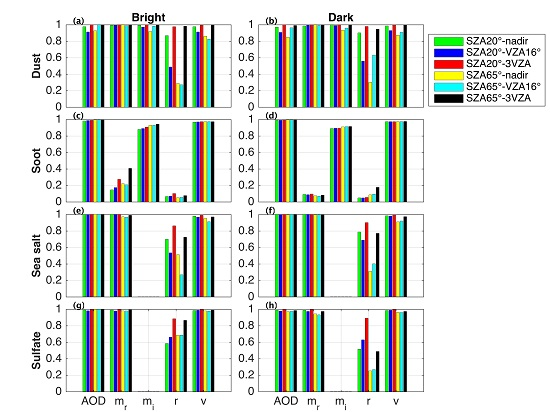
5.1. Influence of Observation Geometry

Figure 3 shows the DFS of each retrieved aerosol parameter for different observation geometries in both nadir viewing mode and target mode. It is clear that the DFS of AOD and PSD variance for all aerosol types are close to 1.0, while the DFS of the real and imaginary parts of the refractive indices and PSD mode radius are less and dependent on aerosol type. For example, among four aerosol types in the retrieval at nadir viewing with small SZA (20°), dust has the largest total information with 4.81 DFS, while the total DFS for soot is the smallest, only 3.05 (Figure 3). The difference of DFS between different aerosol types is determined by their scattering properties (Figure 2) and indicates the sensitivity of CAPI measurement to aerosol properties.

The ground pixels in the wide FOV of CAPI will be observed at different VZA (from 0°–16°) or different SZA. The viewing geometry can lead to some changes in aerosol information due to different aerosol scattering phase functions when scattering angle varies. Thus, we also compare the impact of different viewing geometries on the information obtained regarding aerosol parameters in Figure 3. For example, for dust at 20° SZA, DFS at the forward 16° VZA (blue bar) is lower than that at nadir, which is consistent with the lower scattering phase function at VZA of 16° (Figure 2). However, the DFS of soot for the four viewing scenarios in the nadir observation in our simulation are similar, due to the rather uniform distribution of its scattering phase function (Figure 2). Similarly, the comparison of the DFS at the same VZA, but different SZA (green and yellow bars in Figure 3) also proves the consistent relationship between phase function and aerosol DFS.

In addition to considering the vegetation fraction of surface albedo in the state vector, we also compare the DFS over two surface albedos, the bright and dark surface defined in Section 4, in Figure 3. Consistent with the sensitivity to AOD shown in Figure 1, the DFS for soot over the dark surface at 20° SZA is smaller than that over the bright surface due to less sensitivity (less absolute value of Jacobians at 0.5 × α(λ), such as the red markers in Figure 1). Similarly, the larger DFS for dust and sea salt at 20° SZA over the dark surface correspond to larger Jacobians (black and green markers in Figure 1). Therefore, although the wavelength dependence of surface albedo remains unchanged, the surface albedo value could still have an impact on aerosol information content.

5.2. Improvement of Multi-Angle Measurement

In target mode, to validate satellite data with ground-based observation, TanSat can monitor the same location several times along an orbit. Therefore, several measurements of different viewing geometries for a specific ground pixel can be combined to improve the aerosol retrieval information and accuracy, similar to what has been achieved for POLDER [53]. For simplicity, three along-track measurements at the forward VZA 16°, backward VZA 16° and nadir viewing angles are combined for the multi-angle retrieval. From Figure 3, it is clear that the DFS in multi-angle mode increase compared to the single-view nadir mode result (such as the red and green bars). The additional information acquired in the multi-angle mode is most striking for the PSD mode radius, whose DFS is limited in nadir viewing and can be enhanced 0.22 on average. For the other parameters, we obtain a large amount of information at only-nadir viewing, so the improvement of multi-angle retrieval is not obvious. However, this improvement for soot is so little that only another 0.04 DFS is provided for the PSD mode radius. This situation can be explained by the weak scattering of soot and the small change of phase function in the chosen geometries. Generally, the DFS of the multi-angle retrieval of dust reaches 4.97, indicating we can retrieve almost all five aerosol parameters independently in multi-angle mode. For sea salt and sulfate, the total DFS are 3.85 and 3.87 in the multi-angle mode, respectively, so we can obtain a large amount of information for the four parameters other than the imaginary part of the refractive index. Unfortunately, for soot, the DFS is still only 3.25 in the multi-angle mode, and the ability to retrieve the real part of the refractive index and PSD radius is not improved. In summary, the DFS in multi-angle retrieval increases by 0.31, on average, compared to the nadir mode.

6. Error Analysis and Correlation Matrix for Aerosol Retrieval

In the previous section, we focused on the ability to retrieve aerosol properties from CAPI measurements. Another crucial issue to be considered is the source of error in this retrieval. In this section, we discuss the a posteriori error covariances, $\widehat{S}$, and analyze its sources of a priori uncertainty and measurement noise, respectively, for all of the scenarios described in Section 5. Model parameter uncertainties only related to aerosol profile parameters (half-width, peak-height) are also taken into consideration. The impact of different observation geometries and satellite operational modes are presented. Finally, an error correlation matrix between all of the retrieved parameters is derived, to analyze the correlation between the surface and aerosol parameters.

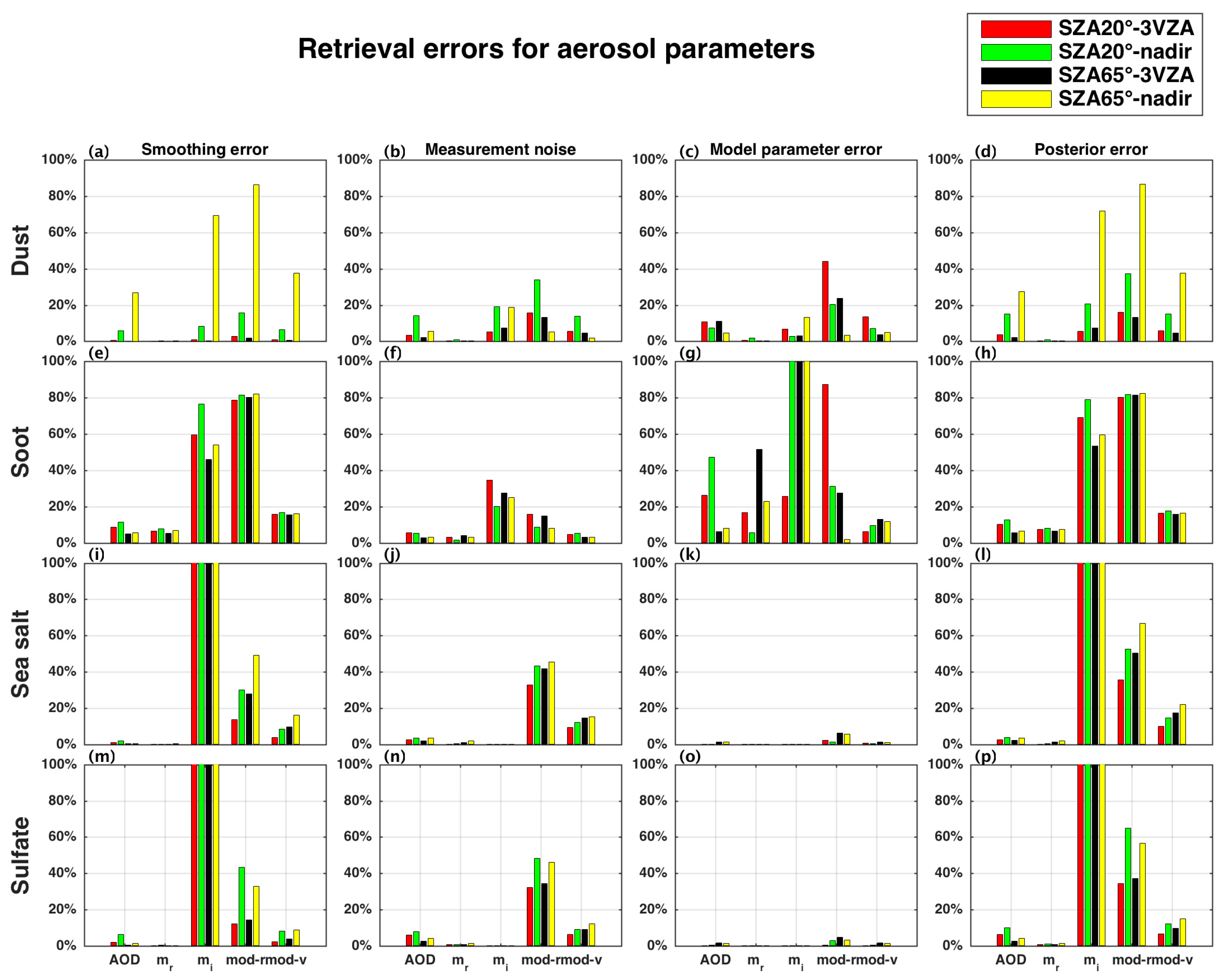
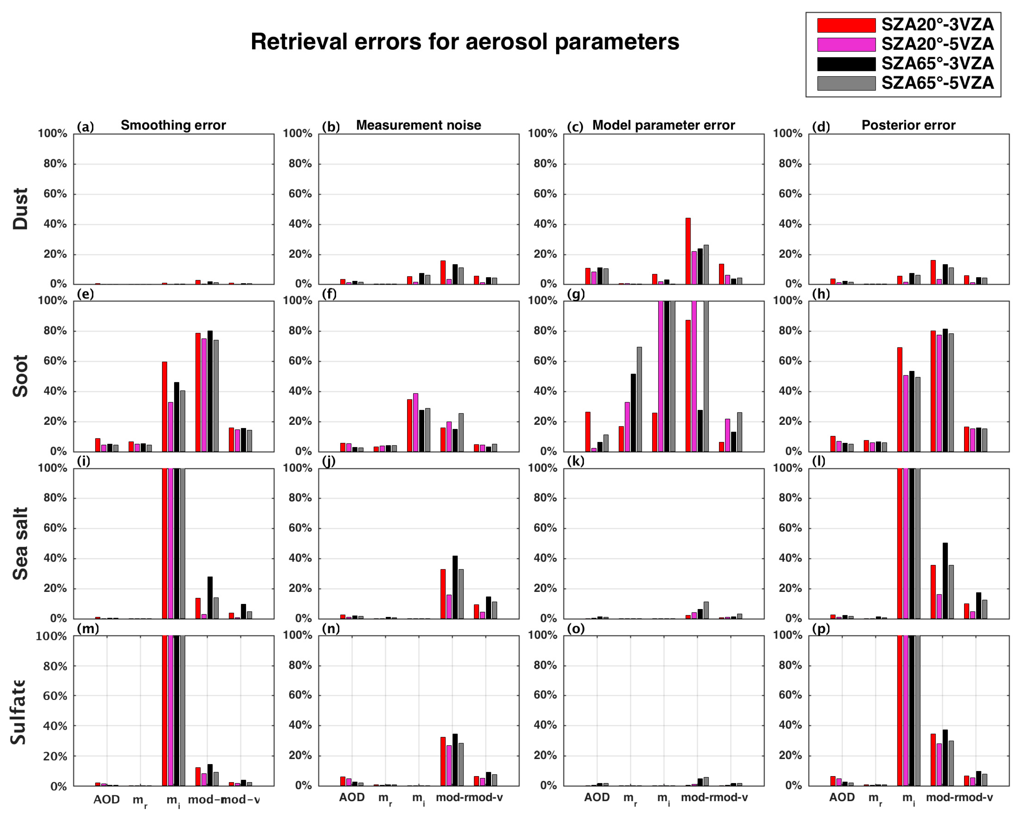
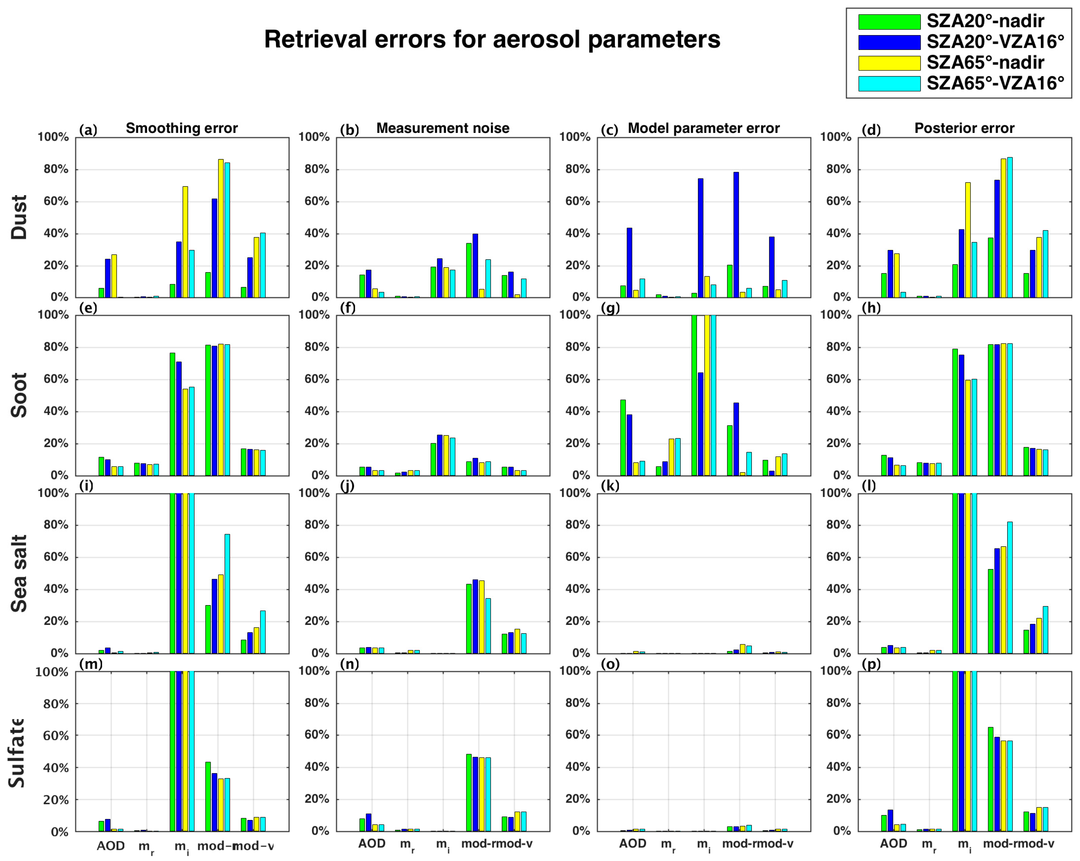
6.1. Retrieval Error and Its Components

From Figure 4 and Figure 5, it can be seen that the patterns of posterior errors and the corresponding smoothing errors are similar for all aerosol types. This implies that the a priori uncertainties rather than measurement noise are the dominated component of the posterior error. We also note that among all retrieved parameters, the imaginary part of the refractive index and the PSD mode radius have the largest posterior errors in nadir mode, i.e., 78% and 70% on average. Therefore, the retrieval accuracy of these two parameters cannot be guaranteed. Actually, for aerosols with little absorption, i.e., sea salt and sulfate, the DFS of the imaginary part of the refractive index are close to zero (Figure 3c,d), and the posterior errors are almost 100% (Figure 4l,p and Figure 5l,p); therefore, this parameter cannot be retrieved from measurements. In other words, its information is mainly from a priori, and the measurement noise has little effect on this parameter (Figure 4j,n and Figure 5j,n).

In addition to a posteriori error, measurement noise and smoothing errors, forward model parameter uncertainties from two aerosol profile parameters are also investigated in Figure 4 and Figure 5. The apparent low values of these errors for sea salt and sulfate indicate that the inaccuracy in depicting the shape of the aerosol profile has little impact on the retrieval uncertainty for these two aerosols. The corresponding model parameter errors for dust and soot are larger, mainly because radiation in the UV band is sensitive to the height of aerosols with absorption.

Furthermore, we also note that in Figure 4, when the scattering phase function is larger at certain observation angles, lower retrieval errors are derived. However, purely noise-related errors are more random. From Figure 5, it is found that the use of three measurements in retrieval can effectively reduce posterior and smoothing errors, especially for those parameters with large errors. The posterior error of the PSD mode radius is reduced the most (23% on average), while the least improvement is achieved for the real part of the refractive index (less than 1%). Among all of the aerosols, the improvement of the multi-angle mode is most apparent for dust (76%), in relation to the large variability of its scattering phase function over the range of our sampled scattering angles. Similarly, the least improvement is achieved for soot (only 10%) due to both the small scattering property and the comparatively uniform phase function.

If another two measurements (forward VZA 30° and backward VZA 30°) are added in multi-angle retrieval, the retrieval errors will be reduced to a greater extent. Figure 6 shows that smoothing errors, and posterior errors are all improved again when five measurements are used in the retrieval. Measurement noise is also reduced, except for soot. Thus, adding more measurements in aerosol retrieval is not an efficient method to improve measurement noise for soot. For dust, which had the greatest improvement in multi-angle retrieval, the smoothing errors are less than 0.1% and almost can be ignored; meanwhile, the average posterior errors are as low as 3% when the number of measurement angles reaches five. The posterior errors for soot, sea salt and sulfate decrease by 4%, 6% and 2% on average, respectively. Finally, we find that a larger number of retrieval measurements can result in less smoothing and posterior errors, impacting on aerosols, especially dust.

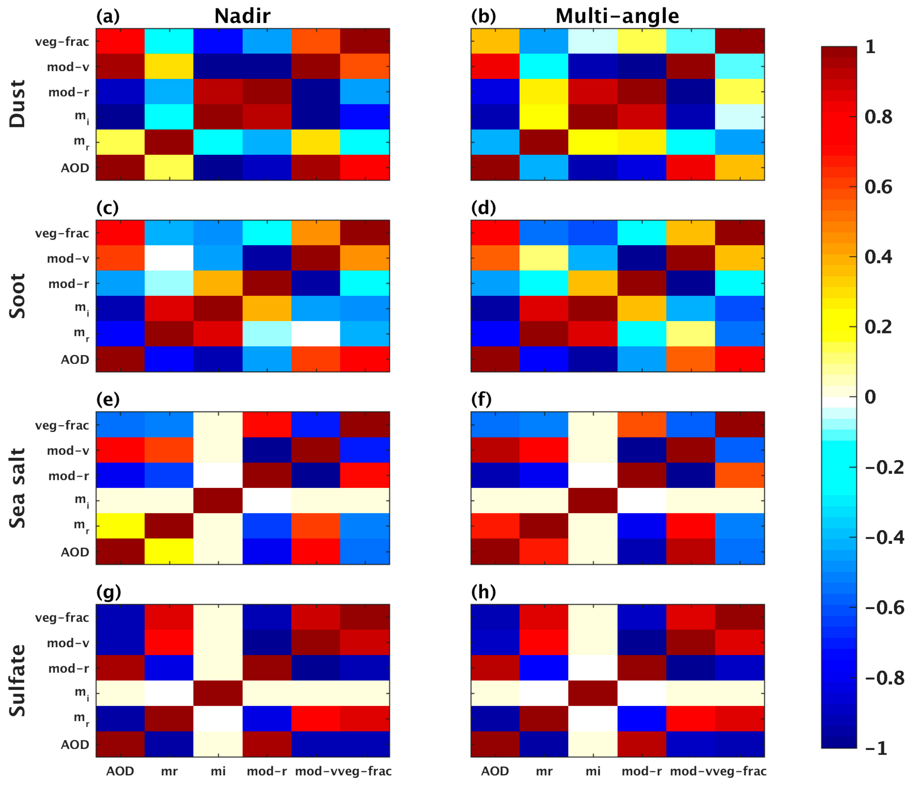
6.2. Correlation of Surface and Aerosol

The error correlation matrices for elements of the state vector are shown in Figure 7. Our main objective is to study the correlation of surface and aerosol parameters (coefficient of vegetation fraction and AOD) and to analyze the strength of the correlation between surface reflection and aerosol scattering. The larger the correlation coefficient, the harder it is to separate the radiative effect from surface and aerosol. For all aerosols, the correlation coefficients between the vegetation fraction and AOD are not less than 0.6, indicating that surface reflection has some influence on aerosol retrieval. However, the correlation coefficients are positive for dust and soot, whereas negative for sea salt and sulfate. If the vegetation fraction is large, the surface albedo decreases, thereby resulting in a diminution of the radiance at TOA. When AOD increases, more scattering for sea salt and sulfate can lead to an enhancement of the radiance at the TOA. Thus, the vegetation fraction and AOD for non-absorbing sea salt and sulfate correlate negatively. When comparing nadir and multi-angle retrieval, the correlation of AOD and the vegetation fraction decreases to less than 0.4 for dust in multi-angle measurements. However, there is no obvious distinction for the other three types of aerosols. This proves that multi-angle retrieval can reduce the correlation between surface reflection and aerosol scattering for a strong scattering aerosol.

7. Conclusions

In this study, we have investigated the potential to retrieve aerosol properties and the analysis of sources of retrieval errors, based on numerical experiments using simulated observations in five bands of CAPI on board TanSat. A forward model comprising a linearized Mie code, a trace gas absorption and Rayleigh scattering model, a surface parameterization and a linearized vector radiative transfer model are introduced. In the simulations, we assume a mono-modal aerosol, with a lognormal PSD and a Gaussian-model aerosol profile distribution. The retrieved parameters include five aerosol properties and one surface parameter. The Jacobians of simulated radiances and polarizations with respect to AOD at different observation geometries are discussed. The retrieval sensitivity specified by the DFS and the retrieval errors are analyzed and compared at different viewing geometries, as well as with multi-angle retrieval for four of the main components of the natural mixed aerosol.

In the nadir view mode of CAPI, we find that of all of the retrieval parameters, the lowest DFS is obtained for the PSD mode radius (0.55 on average), as well as large posterior error (70%), while the DFS for AOD is always close to 1.0. The range of the total DFS from 3.05–4.83 and the variability of retrieval errors among the different aerosol types confirm the sensitivity of CAPI observations to aerosol microphysical properties.

When retrieval is performed with measurements at three along-track viewing angles (±16°, nadir), there is additional information for all aerosol properties, with the average increase of the DFS being 0.31 and the posterior error reduced by a maximum of 23%. By adding another two measurements from other viewing geometries in the retrieval, the aerosol information obtained is improved, and the posterior error can decrease again, from 2%–6%, showing that it is worthwhile to fly CAPI in target mode instead of nadir-only mode. When CAPI works in nadir viewing, the different VZA in the wide FOV of the satellite has little impact on the aerosol information and retrieval error, related to the aerosol phase function. In addition to posterior error, we also analyze the smoothing errors, instrument noise and forward model parameter errors. The results show that the a priori uncertainty is the dominating source of posterior error. Moreover, retrieval errors for sea salt and sulfate are not sensitive to the inaccuracies of aerosol profile distribution, but they result in large errors for dust and soot. Additionally, not only the dependence of surface albedo on wavelength, but also the surface albedo value affects aerosol information content. The error correlation coefficients between the surface parameter and AOD for all aerosols indicate that their different optical properties result in a different strength of correlation between surface reflection and aerosol effects. Multi-angle retrieval can reduce this correlation too some extent for dust.

In recent CO₂ retrieval algorithms, an aerosol model has been added to produce a realistic atmosphere, and the performance of imperfect characterization of the aerosol is proven dominative in CO₂ retrieval uncertainties [11]. Thus, aerosol properties synchronously retrieved from CAPI measurements could help to reduce CO₂ retrieval errors for TanSat. It should be noted that the analysis of the retrieval of aerosol properties and error sources in this study is preliminary and accounts only for the impact of different observation geometries and the number of angles for multi-angle observation, as well as a number of pure aerosol types. The effect of aerosols on high precision greenhouse gas retrieval will be considered in future studies. More complex aerosol and surface models that reflect reality more closely will also be considered.

References

1. Bovensmann, H.; Burrows, J.P.; Buchwitz, M.; Frerick, J.; Noe’l, S.; Rozanov, V.V. SCIAMACHY mission objectives and measurement modes. J. Atmos. Sci. 1999, 56, 127–150. [Google Scholar] [CrossRef]
2. Buchwitz, M.; de Beek, R.; Burrows, J.P.; Bovensmann, H.; Warneke, T.; Notholt, J.; Meirink, J.F.; Goede, A.P.H.; Bergamaschi, P.; Kärner, S.; et al. Atmospheric methane and carbon dioxide from SCIAMACHY satellite data: Initial comparison with chemistry and transport models. Atmos. Chem. Phys. 2005, 5, 941–962. [Google Scholar] [CrossRef]
3. Chahine, M.T.; Pagano, T.S.; Aumann, H.H.; Atlas, R.E.A. AIRS: Improving weather forecasting and providing new data on greenhouse gases. Bull. Am. Meteorol. Soc. 2006, 87, 911–926. [Google Scholar] [CrossRef]
4. Crevoisier, C.; Heilliette, S.; Chédin, A.; Serrar, S.; Armante, R.; Scott, N.A. Midtropospheric CO2 concentration retrieval from AIRS observations in the tropics. Geophys. Res. Lett. 2004, 31. [Google Scholar] [CrossRef]
5. Kuze, A.; Suto, H.; Nakajima, M.; Hamazaki, T. Thermal and near infrared sensor for carbon observation Fourier-Transform Spectrometer on the greenhouse gases observing satellite for greenhouse gases monitoring. Appl. Opt. 2009, 48, 6716–6733. [Google Scholar] [CrossRef] [PubMed]
6. Crisp, D.; Atlas, R.M.; Breon, F.-M.; Brown, L.R.; Burrows, J.P.; Ciais, P.; Connor, B.J.; Doney, S.C.; Fung, I.Y.; Jacob, D.J. The Orbiting Carbon Observatory (OCO) mission. Adv. Space Res. 2004, 34, 700–709. [Google Scholar] [CrossRef]
7. Chen, W.; Zhang, Y.; Yin, Z.; Zheng, Y.; Yan, C.; Yang, Z. In the tansat mission: Global CO2 observation and monitoring. In Proceedings of the 63rd International Astronautical Congress, Naples, Italy, 1–5 October 2012.
8. Liu, Y.; Yang, D.X.; Cai, Z.N. A retrieval algorithm for TanSat XCO2 observation: Retrieval experiments using GOSAT data. Chin. Sci. Bull. 2013, 58, 1520–1523. [Google Scholar] [CrossRef]
9. Yoshida, Y.; Ota, Y.; Eguchi, N.; Kikuchi, N.; Nobuta, K.; Tran, H.; Morino, I.; Yokota, T. Retrieval algorithm for CO2 and CH4 column abundances from short-wavelength infrared spectral observations by the greenhouse gases observing satellite. Atmos. Meas. Tech. 2011, 4, 717–734. [Google Scholar] [CrossRef]
10. Yang, D.; Liu, Y.; Cai, Z. Simulations of aerosol optical properties to top of atmospheric reflected sunlight in the near infrared CO2 weak absorption band. Atmos. Ocean. Sci. Lett. 2013, 6, 60–64. [Google Scholar]
11. O’Dell, C.W.; Connor, B.; Bösch, H.; O’Brien, D.; Frankenberg, C.; Castano, R.; Christi, M.; Eldering, D.; Fisher, B.; Gunson, M.; et al. The ACOS CO2 retrieval algorithm—Part 1: Description and validation against synthetic observations. Atmos. Meas. Tech. 2012, 5, 99–121. [Google Scholar] [CrossRef]
12. Houweling, S.; Hartmann, W.; Aben, I.; Schrijver, H.; Skidmore, J.; Roelofs, G.-J.; Breon, F.M. Evidence of systematic errors in SCIAMACHY-observed CO2 due to aerosols. Atmos. Chem. Phys. 2005, 5, 3003–3013. [Google Scholar] [CrossRef] [Green Version]
13. Ishida, H.; Nakjima, T.Y.; Yokota, T.; Kikuchi, N.; Watanabe, H. Investigation of GOSAT TANSO-CAI cloud screening ability through an intersatellite comparison. J. Appl. Meteorol. Clim. 2011, 50, 1571–1586. [Google Scholar] [CrossRef]
14. Zhang, J.; Shao, J.; Yan, C. Cloud and Aerosol Polarimetric Imager. In Proceedings of the Conferences of the Photoelectronic Technology Committee of the Chinese Society of Astronautics: Optical Imaging, Remote Sensing, and Laser-Matter Interaction, Suzhou, China, 20–29 October 2013.
15. Herman, M.; Deuzé, J.L.; Devaux, C.; Goloub, P.; Bréon, F.M.; Tanré, D. Remote sensing of aerosols over land surfaces including polarization measurements and application to POLDER measurements. J. Geophys. Res. 1997, 102, 17039–17049. [Google Scholar] [CrossRef]
16. Maso, M.D.; Kulmala, M.; Riipinen, I.; Wagner, R.; Hussein, T.; Aalto, P.P.; Lehtinen, K.E.J. Formation and growth of fresh atmospheric aerosols: Eight years of aerosol size distribution data from SMEAR II, Hyytiälä, Finland. Boreal. Environ. Res. 2005, 10, 323–336. [Google Scholar]
17. Hasekamp, O.P.; Landgraf, J. Linearization of vector radiative transfer with respect to aerosol properties and its use in satellite remote sensing. J. Geophys. Res. 2005, 110. [Google Scholar] [CrossRef]
18. Kaufman, Y.J.; Tanré, D.; Remer, L.A.; Vermote, E.F.; Chu, A.; Holben, B.N. Operational remote sensing of tropospheric aerosol over land from EOS Moderate Resolution Imaging Spectroradiometer. J. Geophys. Res. 1997, 102, 17051–17067. [Google Scholar] [CrossRef]
19. Levy, R.C.; Remer, L.A.; Mattoo, S.; Vermote, E.F.; Kaufman, Y.J. Second-generation operational algorithm: Retrieval of aerosol properties over land from inversion of Moderate Resolution Imaging Spectroradiometer spectral reflectance. J. Geophys. Res. 2007, 112. [Google Scholar] [CrossRef]
20. Nagaraja Rao, C.R.; Stowe, L.L.; McClain, E.P. Remote sensing of aerosols over the oceans using AVHRR data theory, practice and applications. Int. J. Remote Sens. 1989, 10, 743–749. [Google Scholar] [CrossRef]
21. Mishchenko, M.I.; Geogdzhayev, I.V.; Cairns, B.; Rossow, W.B.; Lacis, A.A. Aerosol retrievals over the ocean by use of channels 1 and 2 AVHRR data: Sensitivity analysis and preliminary results. Appl. Opt. 1999, 38, 7325–7341. [Google Scholar] [CrossRef] [PubMed]
22. De Graaf, M.; Stammes, P.; Aben, E.A.A. Analysis of reflectance spectra of UV-absorbing aerosol scenes measured by SCIAMACHY. J. Geophys. Res. 2007, 112, 485–493. [Google Scholar] [CrossRef]
23. Torres, O.; Bhartia, P.K.; Herman, J.R.; Sinyuk, A.; Ginoux, P.; Holben, B. A long-term record of aerosol optical depth from TOMS observations and comparison to AERONET measurements. J. Atmos. Sci. 2002, 59, 398–413. [Google Scholar] [CrossRef]
24. Torres, O.; Tanskanen, A.; Veihelmann, B.; Ahn, C.; Braak, R.; Bhartia, P.K.; Veefkind, P.; Levelt, P. Aerosols and surface UV products from ozone monitoring instrument observations: An overview. J. Geophys. Res. 2007, 112. [Google Scholar] [CrossRef]
25. Chiapello, I.; Goloub, P.; Tanré, D.; Marchand, A.; Herman, J.; Torres, O. Aerosol detection by TOMS and POLDER over oceanic regions. J. Geophys. Res. 2000, 105, 7133–7142. [Google Scholar] [CrossRef]
26. Chu, D.A.; Kaufman, Y.J.; Ichoku, C.; Remer, L.A.; Tanre, D.; Holben, B.N. Validation of MODIS aerosol optical depth retrieval over land. Geophys. Res. Lett. 2002, 29. [Google Scholar] [CrossRef]
27. Abdou, W.A.; Diner, D.J.; Martonchik, J.V.; Bruegge, C.J.; Kahn, R.A.; Gaitley, B.J.; Crean, K.A. Comparison of coincident multiangle imaging spectroradiometer and Moderate Resolution Imaging Spectroradiometer aerosol optical depths over land and ocean scenes containing aerosol robotic network sites. J. Geophys. Res. 2005, 110. [Google Scholar] [CrossRef]
28. Diner, D.J.; Beckert, J.C.; Reilly, T.H.; Bruegge, C.J.; Conel, J.E.; Kahn, R.; Martonchik, J.V.; Ackerman, T.P.; Davies, R.; Gerstl, S.A. Multi-angle Imaging Spectroradiometer (MISR) instrument description and experiment overview. IEEE Trans. Geosci. Remote Sens. 1998, 36, 1072–1087. [Google Scholar] [CrossRef]
29. Kahn, R.A.; Gaitley, B.J.; Martonchik, J.V.; Diner, D.J.; Crean, K.A. Multiangle Imaging Spectroradiometer (MISR) global aerosol optical depth validation based on 2 years of coincident aerosol robotic network (AERONET) observations. J. Geophys. Res. 2005, 110, 1–16. [Google Scholar] [CrossRef]
30. Liu, Y.; Koutrakis, P.; Kahn, R. Estimating fine particulate matter component concentrations and size distributions using satellite-retrieved fractional aerosol optical depth: Part 1—Method development. J. Air Waste Manag. Assoc. 2007, 57, 1351–1359. [Google Scholar] [PubMed]
31. Hansen, J.E.; Travis, L.D. Light scattering in planetary atmospheres. Space Sci. Rev. 1974, 16, 527–610. [Google Scholar] [CrossRef]
32. Leroy, M.; Deuze, J.L.; Breon, F.M.; Hautecoeur, O.; Herman, M.; Buriez, J.C.; Tanre, D.; Bouffies, S.; Chazette, P.; Roujean, J.L. Retrieval of atmospheric properties and surface bidirectional reflectances over land from POLDER/ADEOS. J. Geophys. Res. 1997, 102, 17023–17037. [Google Scholar] [CrossRef]
33. Deuzé, J.L.; Bréon, F.M.; Devaux, C.; Goloub, P.; Herman, M.; Lafrance, B.; Maignan, F.; Marchand, A.; Nadal, F.; Perry, G.; et al. Remote sensing of aerosols over land surfaces from POLDER-ADEOS-1 polarized measurements. J. Geophys. Res. 2001, 106, 4913–4926. [Google Scholar] [CrossRef]
34. Hasekamp, O.P.; Landgraf, J. Retrieval of aerosol properties over land surfaces: Capabilities of multiple-viewing-angle intensity and polarization measurements. Appl. Opt. 2007, 46, 3332–3344. [Google Scholar] [CrossRef] [PubMed]
35. Sinyuk, A.; Dubovik, O.; Holben, B.; Eck, T.F.; Breon, F.-M.; Martonchik, J.; Kahn, R.; Diner, D.J.; Vermote, E.F.; Roger, J.-C.; et al. Simultaneous retrieval of aerosol and surface properties from a combination of AERONET and satellite data. Remote. Sens. Environ. 2007, 107, 90–108. [Google Scholar] [CrossRef]
36. Torres, O. Total Ozone Mapping Spectrometer measurements of aerosol absorption from space: Comparison to SAFARI 2000 ground-based observations. J. Geophys. Res. 2005, 110. [Google Scholar] [CrossRef]
37. Torres, O.; Ahn, C.; Chen, Z. Improvements to the OMI near-UV aerosol algorithm using A-Train CALIOP and AIRS observations. Atmos. Meas. Tech. 2013, 6, 3257–3270. [Google Scholar] [CrossRef]
38. Frankenberg, C.; Hasekamp, O.; O’Dell, C.; Sanghavi, S.; Butz, A.; Worden, J. Aerosol information content analysis of multi-angle high spectral resolution measurements and its benefit for high accuracy greenhouse gas retrievals. Atmos. Meas. Tech. 2012, 5, 1809–1821. [Google Scholar] [CrossRef]
39. Butz, A.; Hasekamp, O.P.; Frankenberg, C.; Aben, I. Retrievals of atmospheric CO2 from simulated space-borne measurements of backscattered near-infrared sunlight: Accounting for aerosol effects. Appl. Opt. 2009, 48, 3322–3336. [Google Scholar] [CrossRef] [PubMed]
40. Wang, J.; Xu, X.; Ding, S.; Zeng, J.; Spurr, R.J.D.; Liu, X.; Chance, K.; Mishchenko, M.I. A numerical testbed for remote sensing of aerosols, and its demonstration for evaluating retrieval synergy from a geostationary satellite constellation of GEO-CAPE and GOES-R. J. Quant. Spectrosc. Radiat. 2014, 146, 510–528. [Google Scholar] [CrossRef]
41. Chen, X.; Wang, J.; Liu, Y.; Xu, X.; Cai, Z.; Yang, D.; Yan, C.-X. Angular dependence of aerosol information content in CAPI/TanSat observation over land: Effect of polarization and synergy with A-Train satellites. Remote. Sens. Environ. 2016. under review. [Google Scholar]
42. Martynenko, D.; Holzer-Popp, T.; Elbern, H.; Schroedter-Homscheidt, M. Understanding the aerosol information content in multi-spectral reflectance measurements using a synergetic retrieval algorithm. Atmos. Meas. Tech. 2010, 3, 1589–1598. [Google Scholar] [CrossRef] [Green Version]
43. Geddes, A.; Bösch, H. Tropospheric aerosol profile information from high-resolution oxygen A-band measurements from space. Atmos. Meas. Tech. 2015, 8, 859–874. [Google Scholar] [CrossRef]
44. Spurr, R.J.D.; Wang, J.; Zeng, J.; Mishchenko, M.I. Linearized T-matrix and Mie scattering computations. J. Quant. Spectrosc. Radiat. 2012, 113, 425–439. [Google Scholar] [CrossRef]
45. Hess, M.; Koepke, P.; Schult, I. Optical Properties of Aerosols and Clouds: The software package OPAC. Bull. Am. Meteorol. Soc. 1998, 79, 831–844. [Google Scholar] [CrossRef]
46. Bodhaine, B.A.; Wood, N.B.; Dutton, E.G.; Slusser, J.R. On Rayleigh optical depth calculations. J. Atmos. Ocean. Technol. 1999, 16, 1854–1861. [Google Scholar] [CrossRef]
47. Rothman, L.S.; Gordon, I.E.; Barbe, A.; Benner, D.C.; Bernath, P.F.; Birk, M.; Boudon, V.; Brown, L.R.; Campargue, A.; Champion, J.P.; et al. The HITRAN 2008 molecular spectroscopic database. J. Quant. Spectrosc. Radiat. 2009, 110, 533–572. [Google Scholar] [CrossRef]
48. Von Hoyningen-Huene, W.; Freitag, M.; Burrows, J.B. Retrieval of aerosol optical thickness over land surfaces from top-of-atmosphere radiance. J. Geophys. Res. 2003, 108. [Google Scholar] [CrossRef]
49. Meer, F.V.D.; Jong, S.M.D. Improving the results of spectral unmixing of landsat thematic mapper imagery by enhancing the orthogonality of end-members. Int. J. Remote. Sens. 2000, 21, 2781–2797. [Google Scholar] [CrossRef]
50. Yamaguchi, Y.; Kahle, A.B.; Tsu, H.; Kawakami, T.; Pniel, M. Overview of advanced spaceborne thermal emission and reflection radiometer (ASTER). Geosci. Remote Sens. 1998, 36, 1062–1071. [Google Scholar] [CrossRef]
51. Spurr, R. Lidort and vlidort: Linearized pseudo-spherical scalar and vector discrete ordinate radiative transfer models for use in remote sensing retrieval problems. In Light Scattering Reviews 3; Kokhanovsky, D.A.A., Ed.; Springer: Berlin/Heidelberg, Germany, 2008; pp. 229–275. [Google Scholar]
52. Spurr, R.J.D. Vlidort: A linearized pseudo-spherical vector discrete ordinate radiative transfer code for forward model and retrieval studies in multilayer multiple scattering media. J. Quant. Spectrosc. Radiat. 2006, 102, 316–342. [Google Scholar] [CrossRef]
53. Mukai, S.; Sano, I. Retrieval algorithm for atmospheric aerosols based on multi-angle viewing of ADEOS/POLDER. Earth Planets Space 1999, 51, 1247–1254. [Google Scholar] [CrossRef]
Figure 1. Jacobians of AOD in all channels of CAPI at four viewing angles (0°, 16°, 30°, 60°) and 20° solar zenith angle (SZA) with a bright and a dark surface for four types of aerosols. (ac) represent Jacobians at 380 nm, 870 nm and 1375 nm, respectively. (df) and (gi) are polarized Jacobians of Stokes vector I, Q and U at 670 nm and 1640 nm, respectively. The black, red, green and blue markers mean radiance or polarization for dust, soot, sea salt and sulfate, respectively. The asterisks represent the bright surface with albedo α(λ), and squares mean the dark surface with 0.5 × α(λ) as albedo. The thin blue dashed line represents zero Jacobian.
Remotesensing 09 00183 g001
Figure 2. Scattering phase functions of four aerosol types used in this study. Black, red, green and yellow thick solid lines represent the scattering phase function of dust, soot, sea salt and sulfate. Scattering angles corresponding to different solar zenith angles and viewing zenith angles are indicated by cyan and blue thin solid or dashed lines, respectively. VZA, viewing zenith angle.
Remotesensing 09 00183 g002
Figure 3. The degrees of freedom for the signal (DFS) of corresponding aerosol parameters at different viewing angles in high and low solar zenith angles for four types of aerosol over the bright and dark surface defined as in Section 4. The left column is for the bright surface, and the right column is for the dark surface. Four rows represent four aerosol types: dust (a,b), soot (c,d), sea salt (e,f) and sulfate (g,h). Different colored bars represent corresponding different observation geometries. The X-axis represents five retrieved aerosol parameters: AOD, real (mr) and imaginary part of refractive index (mi), mode radius (mod-r) and variance (mod-v) of PSD.
Remotesensing 09 00183 g003
Figure 4. Different error estimates (1σ) of aerosol parameters at different observation geometries for all aerosols. Each row represents one type of aerosol: dust (ad), soot (eh), sea salt (il) and sulfate (mp), respectively. The range of ordinate represents percentage.
Remotesensing 09 00183 g004
Figure 5. Different error estimates (1σ) of aerosol parameters at different solar zenith angles in nadir and multi-angle mode. Others are the same as Figure 4.
Remotesensing 09 00183 g005
Figure 6. Four kinds of retrieval errors for multi-angle retrieval in three viewing angles and five viewing angles respectively. Others are the same as Figure 4.
Remotesensing 09 00183 g006
Figure 7. The correlation matrices of retrieval variables for four types of aerosols (four rows): dust (a,b), soot (c,d), sea salt (e,f) and sulfate (g,h). The left column is in nadir viewing mode, and the right column is in multi-angle mode.
Remotesensing 09 00183 g007