Improving Winter Wheat Yield Estimation from the CERES-Wheat Model to Assimilate Leaf Area Index with Different Assimilation Methods and Spatio-Temporal Scales

Abstract

To improve the accuracy of winter wheat yield estimation, the Crop Environment Resource Synthesis for Wheat (CERES-Wheat) model with an assimilation strategy was performed by assimilating measured or remotely-sensed leaf area index (LAI) values. The performances of the crop model for two different assimilation methods were compared by employing particle filters (PF) and the proper orthogonal decomposition-based ensemble four-dimensional variational (POD4DVar) strategies. The uncertainties of wheat yield estimates due to different assimilation temporal scales (phenological stages and temporal frequencies) and spatial scale were also analyzed. The results showed that, compared with the crop model without assimilation and with PF-based assimilation, a better yield estimate performance resulted when the POD4DVar-based strategy was used at the field scale. When using this strategy, root mean square errors (RMSE) of 523 kg·ha⁻¹, 543 kg·ha⁻¹ and 172 kg·ha⁻¹ and relative errors (RE) of 5.65%, 5.91% and 7.77% were obtained at the field plot scale, a pixel scale of 1 km and the county scale, respectively. Although the best yield estimates were obtained when all of the observed LAIs were assimilated into the crop model, an acceptable estimate of crop yield could also be achieved by assimilating fewer observations between jointing and anthesis periods of the crop growth season. With decreasing assimilation frequency and pixel resolution, the accuracy of the crop yield estimates decreased; however, the computation time decreased. Thus, it is important to consider reasonable spatio-temporal scales to obtain tradeoffs between accuracy and effectiveness in regional wheat estimates.

1. Introduction

Timely and accurate regional crop growth monitoring and yield forecasting play a significant role in guiding agricultural production, ensuring national food security and maintaining sustainable agriculture development [1,2,3,4]. In the past few decades, conventional agro-meteorological models and empirical statistical regression models based on field-measured yields and related remotely-sensed spectral vegetation indices [5] were used to monitor crop growth and yields, with the disadvantages of high-cost, laboriousness, inefficiency and only being applicable for local regions [6,7,8]. Process-oriented crop growth models can offer powerful tools to simulate the crop growth and obtain the crop yield under various environmental and management conditions with the advantages of cost, timeliness, accuracy and suitability at the field scale [6,9,10,11,12,13,14], while they were also dynamically accounting for several limiting factors (e.g., soil, weather, water, nitrogen and field management data) at the regional scale [3,15]. With the development of remote sensing technology, extensive remotely-sensed data provide a synopsis of timely and up-to-date crop growing conditions over large areas throughout the crop’s growing season and can be employed to provide many potential data for crop model simulations [16]. Therefore, data assimilation approaches that integrate crop growth models with remote sensing data have been proposed recently and recognized as important approaches for monitoring crop growth conditions and improving the accuracy of yield estimations at the regional scale [6,7,9,17,18,19,20,21,22,23,24,25].

Commonly, there are two main kinds of strategies for data assimilation to reduce the discrepancy between observations and simulations by adjusting the initial model conditions, parameters (e.g., canopy and growth parameters) [7,17,21] or model state variables [3,10,26]: (1) recalibration/re-initialization methods and (2) state-updating methods [27]. The recalibration methods can be carried out using optimization algorithms (e.g., Price [19,28], Powell [29,30], simulated annealing (SA) [31], the shuffled complex evolution method developed at the University of Arizona (SCE-UA) [32], etc. [33,34]) to re-initialize or re-parameterize a crop growth model to minimize the merit function between modeled parameters and remotely-sensed parameters. However, the disadvantages of these methods are that they could not consider uncertainties in observations, and the model itself, usually failing to capture and maintain the crop system dynamics, and the iterative process may require excessive computing time [4,7,34,35]. Thus, the state-updating methods carried out using assimilation algorithms (e.g., an ensemble Kalman filter (EnKF) [3,10,36,37], particle filters (PF) [22,38,39], traditional variational methods [40,41] or ensemble-based four-dimensional variation [9,42,43], etc.) were introduced into crop growth simulations to alleviate the shortcomings of the recalibration/re-initialization methods and can combine many types of observations at random times, and the state variables can also be continually updated and simulated accurately [4]. Especially EnKF, as one of the typical state-updating methods, has received much attention because of its simple conceptual formulation and relative ease of implementation [3,10,21,36,41]. However, the disadvantages of this method are that it may result in an obvious deficiency when solving complicated estimation issues in a nonlinear and non-Gaussian dynamic system, and it also has low computational efficiency since it is designed to incorporate sequential information only [9].

To solve these problems associated with the EnKF, PF have received increasing attention thanks to their improved performance. Similar to EnKF, PF is also a Monte Carlo technique that uses particles to estimate the underlying probability density function (PDF) of model states/parameters [9]. However, in contrast with EnKF, PF does not rely on the Gaussian assumption of distributions, can perfectly accommodate the propagation of non-Gaussian distributions through nonlinear models [39,44,45,46,47,48] and is thus adapted to the potentially highly nonlinear crop models [49,50]. Accordingly, the PF algorithm appears to be a better choice for complicated crop growth models. On the other hand, the advantages of the traditional four-dimensional variational (4DVar) methods are that they can provide the temporal smoothness constraint and have the ability to simultaneously assimilate the observational data at multiple times in an assimilation window so that the computational cost is lower than EnKF. However, traditional 4DVar methods also have some challenges in maintaining and updating the adjoint models of the forecast models, and they require linearization of the forecast models [9,41]. To maximally use the advantages of the EnKF and variational data assimilations, while simultaneously offsetting their respective weaknesses, an ensemble 4DVar method is proposed on the basis of the proper orthogonal decomposition (POD) [50]. Although a Gaussian distribution assumption of the posterior density of the simulated variable is also given, this method outperforms both the 4DVar and EnKF methods under various nonlinear and non-Gaussian model scenarios with lower computational costs than EnKF and does not need the adjoint or tangent linear model, and thus, the higher accuracy and computational efficiency of the crop yield estimations would be obtained in crop model data assimilation [9,51]. Accordingly, the assimilation of remotely-sensed information into crop growth models with the POD-based ensemble 4DVar (POD4DVar) has also been presented as a better approach to improve the estimation of regional crop yields. Thus, both the PF- and POD4DVar-based strategies were chosen to assimilate the crop model for estimating the regional crop yields.

When a crop model is used to estimate crop yields early in the growing season, climate and model uncertainties are the two main sources of uncertainties [52,53]. Climate-related uncertainties are greatest early in the growing season, but can be reduced when meteorological data become available [54]. Model-related uncertainties are subject to the model structure, the model assumed and data errors; hence, they are imperfect in simulating the true growth process. Without altering the crop models’ structure, data assimilation can be used to improve the model performance by periodically updating state variables within the growing season with remote sensing observations. Remote sensing of vegetation (e.g., leaf area index (LAI)), as the major indicator for crop models, is potentially useful for data assimilation because of its obvious influence on crop growth and, hence, on crop yields [18,53]. To obtain better estimates of regional crop information, a series of remotely-sensed LAIs during the crop growing season must be accurately estimated [6,22,54]. However, current remote sensing LAI products [55,56,57] have some issues in the practical applications for crop model data assimilation: (1) the observations during the crop growing season are usually limited by cloud coverage, rain and long revisit periods; (2) the high frequencies of observations would need a high computational cost, while the low frequencies at critical crop growth stages may also provide relatively accurate results; (3) the commonly-used LAI data were from single sensors, while data combined from multiple sensors’ LAI results were rarely used for assimilation; and (4) the spatial resolutions of the remotely-sensed LAIs are commonly fairly coarse with mixed pixels [6], which may result in various uncertainties in the spatial distributions of the crop parameters, soil properties, management parameters and, finally, result in poor performance of the assimilation model. Hence, based on the assimilation framework, it is important to obtain the highly accurate, estimated LAI products first, and it is also important to analyze the performance of crop model data assimilation using different assimilation phenological stages, frequencies and spatial scales.

To improve the crop yield estimation and clearly illustrate the influences of the factors described above in the crop model data assimilation, the Crop Environment Resource Synthesis-Wheat (CERES-Wheat) model [58] with PF and POD4DVar-based strategies was used to assimilate LAI from field or multiple sensors’ optical data for wheat yield estimation. The main tasks of this study were to: (1) retrieve LAIs using the PROSAIL model with multiple sensors’ data and validate the accuracy of the estimates; (2) assimilate observations of LAI into the CERES-Wheat model with PF and POD4DVar-based strategies to estimate the wheat yields and compare the performances of these two strategies at the field scale; (3) assimilate observations of LAI into the CERES-Wheat model with the better strategy and analyze the uncertainties of the yield estimates with different temporal scales (i.e., phenological stages and frequencies); and (4) discuss the effects of the spatial scales of LAI at the regional scale. Thus, it is highly beneficial to improve the estimations of the regional winter wheat yields by using an operational system of crop model data assimilation.

2. Materials and Methods

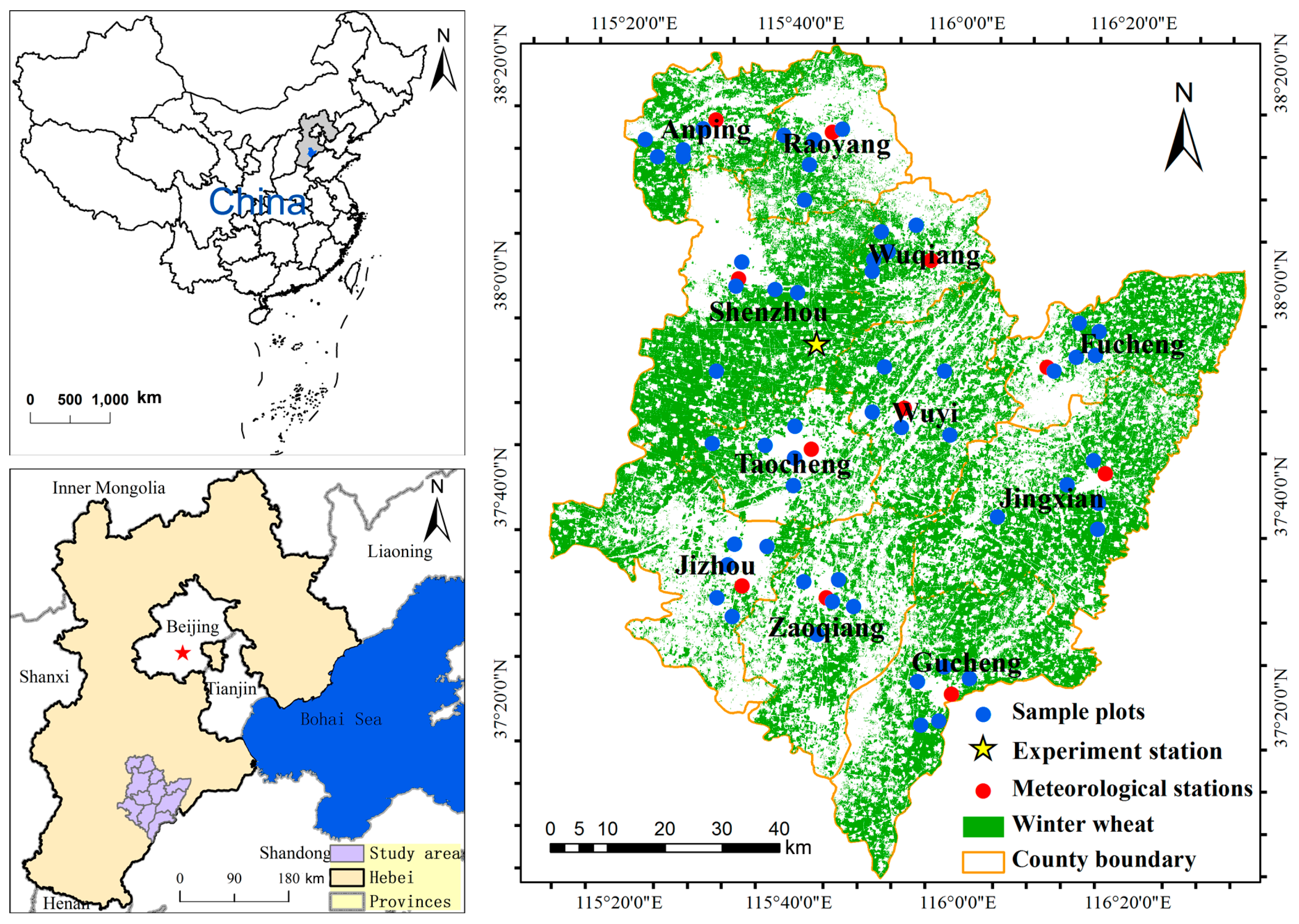
2.1. Study Area

The study was conducted in a planting area dominated by winter wheat in Hengshui City (37°03′–38°23′N, 115°10′–116°34′E), located in the southeast of Hebei province, China. This area covers approximately 8815 km² and consists of 11 counties. The topography of the region is characterized by alluvial plains, and the region of this study area is relatively flat, with an altitude that increases gradually from 12–30 m from southwest to northeast. The climate is a temperate sub-humid continental monsoon climate with average precipitation ranging from 500–900 mm, the annual average temperature ranging from 12–13° C, the annual cumulative temperature above 0 °C ranging from 4200–5500 °C and the annual cumulative radiation ranging from 5.0 × 10³–5.2 × 10³ MJ·m⁻². The soil types mainly consist of the fluvo-aquic soil, sandy fluvo-aquic soil and wet fluvo-aquic soil. The main crops include winter wheat, maize and cotton. High winter wheat yields are traditionally reported from this region, where the soil, climate conditions and adequate irrigation from groundwater make the region suitable for winter wheat growth [6]. For winter wheat, the developmental period occurs from early October to early or mid-June of the next year. The green-up period begins in early March; the jointing stage and elongation stages last from the end of March until mid-April; the booting and heading stages last from the end of April until early May; the anthesis and grain-filling stages begin in early to mid-May; and the harvest usually occurs in early or mid-June. Figure 1 shows the study area and the distribution of the meteorological stations and field sample plots.

2.2. Data Preparation

2.2.1. Field Observation Data

A mechanistic model of CERES-Wheat to simulate crop growth was chose in this study. To calibrate and validate the model for use in our study region, field experiments were performed at the dryland farming and water saving agricultural experimental station, Hebei Academy of Agriculture and Forestry Science, which is located north of Hujiachi Town, in Shenzhou City (Figure 1). Seven field plots were used to derive the crop growth model. The field observations contained the important crop management information (i.e., the dates of planting and harvest, the planting depth and spacing, the planting density, irrigation dates and volumes, fertilization dates and volumes, phenological calendar) and observational yields.

To acquire the growth conditions and validate the inverted LAI for winter wheat at a regional scale during different growth stages, 55 sample plots of the homogenous wheat areas (Figure 1) and seven key phenological stages were selected from March–May 2014: green-up stage (early March), jointing stage (late March), elongation stage (early April), booting stage (late April), heading stage (early May), anthesis stage (mid-May) and maturity (early June). The selected sample plots were located at least 100 m away from roads, residential areas or trees to avoid their influence on the measurements. The area of each sample plot was more than 90 m × 90 m, with three 5 m × 5 m areas measured in each plot, and a Trimble GeoXT3000 GPS from Trimble Navigation, Ltd., Sunnyvale, California, United States of America (USA), was used to locate their position in the field. The wheat LAI were non-destructively measured using an LAI-2000 plant canopy analyzer from LI-COR Inc. (Lincoln, NE, USA) [59]. To prevent direct sunlight on the sensor and minimize the illumination conditions and boundary effects, all measurements were made with the Sun behind the operator, and the operator used a view restrictor of 45°. Finally, LAI values from the three areas were averaged to represent the unique LAI value in each sample plot.

The winter wheat yields in the 55 sample plots were manually measured after harvesting in early June of 2014.

2.2.2. Remote Sensing Data

The optical remotely-sensed data in this study included the images of Chinese Gaofen-1 high-resolution satellite Wide Field Camera (GF-1 WFV), the China environment and disaster monitoring and forecasting small satellite constellation 1A/B satellites charge coupled device (HJ-1A/B CCD) and the Landsat 8 Operational Land Imager (Landsat-8 OLI). The primary sensor characteristics are shown in the

Table 1. The GF-1 WFV (Wide Field Camera), HJ-1 CCD (Charge Coupling Device)and Landsat-8 OLI (Operational Land Imager) specifications.

Sensor	Band	Wavelength Range (μm)	Radiometric Resolution (bit)	Spatial Resolution (m)	Swath (km)	Revisit Period (days)
GF-1 WFV	Blue (1)	0.450–0.520	10	16	200 (1CCD) 800 (4CCD)	4
	Green (2)	0.520–0.590
	Red (3)	0.630–0.690
	Nir (4)	0.770–0.890
HJ-1 CCD	Blue (1)	0.430–0.520	8	30	360 (1CCD) 720 (2CCD)	4
	Green (2)	0.520–0.600
	Red (3)	0.630–0.690
	Nir (4)	0.760–0.900
Landsat-8 OLI	Blue (2)	0.450–0.515	16	30	170 × 185	16
	Green (3)	0.525–0.600
	Red (4)	0.630–0.680
	Nir (5)	0.845–0.885

. Compared with the commonly-used optical remote sensing data, such as the Moderate Resolution Imaging Spectroradiometer (MODIS), these images have good spatial resolutions of less than 30 m, which makes it more suitable to map winter wheat LAI with relatively fragmented areas in Hengshui city. The combination of these multiple sensor images makes it possible to obtain more optical images to cover the study area during the growth periods of winter wheat. In this study, 16 images covering the study area with a high overall quality between March and June in 2014 were acquired, which are listed in

Table 2. Image acquisition information (θ: zenithal angle; ϕ: azimuthal angle).

	Data	Sensor	Time UTC	θsun	ϕsun	θSensor	ϕSensor
1	4 March 2014	HJ-1B CCD2	01 h 58 min	55.97	315.70	12.75	97.00
2	23 March 2014	HJ-1B CCD2	01 h 45 min	49.80	310.44	32.00	97.00
3	3 April 2014	GF-1 WFV4	03 h 42 min	55.67	162.79	63.44	285.08
4	4 April 2014	HJ-1B CCD2	01 h 55 min	45.97	306.82	15.00	98.00
5	8 April 2014	HJ-1B CCD2	01 h 58 min	44.76	305.55	12.70	98.00
6	13 April 2014	Landsat-8 OLI	02 h 54 min	34.85	141.18	0	90
7	14 April 2014	GF-1 WFV1	03 h 12 min	58.12	149.88	63.41	101.48
8	29 April 2014	Landsat-8 OLI	02 h 54 min	38.09	136.81	0	90
9	5 May 2014	HJ-1B CCD2	01 h 54 min	37.93	296.64	22.0	98.00
10	7 May 2014	HJ-1A CCD2	01 h 55 min	37.05	296.71	24.00	97.00
11	12 May 2014	HJ-1A CCD1	02 h 23 min	33.21	298.83	13.00	283.00
12	15 May 2014	Landsat-8 OLI	02 h 54 min	25.33	131.37	0	90
13	17 May 2014	GF-1 WFV2	03 h 18 min	68.51	144.80	74.43	101.31
14	21 May 2014	GF-1 WFV1	03 h 16 min	68.27	141.16	63.39	101.47
15	29 May 2014	HJ-1B CCD1	02 h10 min	31.14	293.58	12.40	282.00
16	5 June 2014	HJ-1B CCD2	01 h 50 min	33.43	286.39	13.30	98.00

.

A series of pre-processing steps was performed using ENVI 5.3 software (Exelis Visual Information Solutions Inc., 4990 Pearl East Cir, Boulder, CO, USA), including radiometric calibration, atmospheric correction and geometric correction, to convert the radiance to reflectance with the correct geographic information.

2.2.3. Soil, Weather and Crop Information

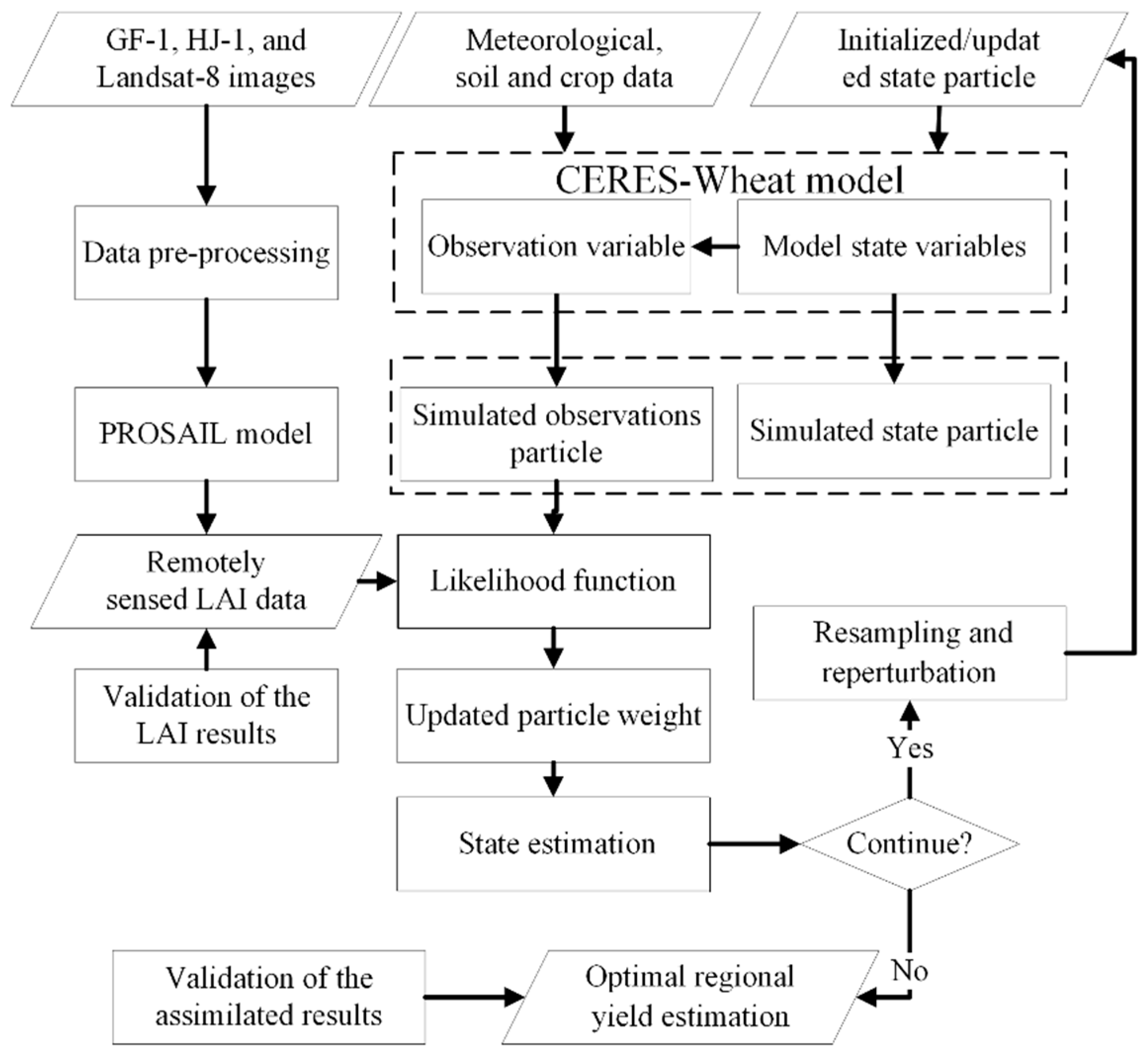
The soil map for the study area was derived from Chinese Soil Science Database for primary Hengshui data at a scale of 1:1,000,000. The map data were compiled based on the soil survey and reference system of the Chinese genetic soil classification system [60,61]. Physical and chemical data from the soil profiles were also obtained from the Chinese Soil Science Database and Soil species of Hebei province [62].

Meteorological data were important external input data to run the CERES-Wheat model and derived from the National Meteorological Information Center, China Meteorological Administration (http://nmic.cn/web/index.htm). The meteorological data observed from 11 meteorological stations at the county level in 2013–2014 included daily maximum and minimum air temperatures, sunshine duration and precipitation. The daily hours of sunshine required conversion into the solar radiation based on the following equations [63]:

$$Q={\mathrm{Q}}_0\left(a+bS/S_0\right)$$

(1)

$$S_0=\frac{24}{\pi }\arccos \left(-\tan \left(\phi \right)\tan \left(\delta \right)\right)$$

(2)

$$a=0.10+0.24S/S_0$$

(3)

$$b=0.38+0.08S/S_0$$

(4)

where a and b are empirical coefficients dependent on the climate and the locality. S/S₀ represents the ratio of actual to potential duration of sunshine. $\phi$ is the geographic latitude of the meteorological stations, while δ represents the declination. Q is the actual daily radiation, and the Q₀ is the incident radiation of the aeropause calculated using the FAO-56 guide [64]. Meteorological information was from reliable meteorological stations, monitored daily, and the study area was relative small. Consequently, the effects of meteorological elements were not considered in this experiment. To regionalize the crop model, the daily meteorological inputs for the study area were spatialized as a raster map with 1-km grid cells using ANUSPLIN software [65].

The spatial distribution map of winter wheat in 2014 was derived from the Key Laboratory of Agri-informatics, Ministry of Agriculture, Beijing, China. The classification results were received based on the GF-1 images and field investigations, and the overall accuracy was higher than 90%.

The regional statistical yields in 2014 for 11 counties were obtained from the agricultural extension stations of Hengshui.

3. Method

3.1. Crop Growth Model

3.1.1. Description of the Crop Growth Model

The CERES-Wheat model was developed and integrated into the Decision Support System for Agro-technology Transfer (DSSAT) software in the International Benchmark Sites for Agro-technology Transfer project (IBSNAT) sponsored by the United States Department of Agriculture (USDA) [58]. The model is a mechanistic process-based model and uses a generic process description that is suitable for large-scale and regional simulations by the strategy of data assimilation. The model has been widely applied to assess potential crop productivity, determine the influences of climate change on grain yields, farmland water and fertilizer management [66,67]. Thus, this model was selected to estimate the yield of winter wheat in this study.

Driven by input data on soil, meteorological data, genetic information and field management, the CERES-Wheat model can simulate daily phenological development, vegetative and reproductive plant developmental stages, biomass accumulation and ultimate yield [22,33]. In this model, the yield is simulated as a function of the grain weight. Grain growth is developmentally dependent on the wheat daily growth, which is a function of the mean daily temperature and daily cumulative solar radiation, a temperature control factor, vegetation biomass and the model parameters [68]. Given the way in which the model develops the vegetation and grain components of the wheat plant, the LAI will determine yield based on the vegetation biomass [33].

3.1.2. Calibration of Crop Growth Model

The CERES-Wheat model requires data on a range of parameters (containing at least four meteorological parameters, 18 soil parameters, nine management parameters and 33 crop parameters) for each cell in the grid to simulate the spatial distribution of crop yield [58]. Before using a crop model for a given region, the calibration should be firstly carried out, and the performance of the calibration should be evaluated to ensure that the model can accurately simulate the crop growth process by accounting for the variability of various local environmental parameters and the characteristics of the wheat [6].

Sensitivity analysis is an effective way to solve the above issues and to evaluate the uncertainty of the crop model quantitatively. This method investigates how the uncertainties of the model’s estimates are related to its input parameters, so as to rank the parameters' influence on the uncertainty of the model's output and finding the key parameters. In this study, a global sensitivity analysis was performed using the extended Fourier amplitude sensitivity test method (EFAST) [69] to analyze the most sensitive parameters in the CERES-Wheat model, with the goal of identifying the most important parameters to be calibrated. Using Simlab software from Joint Research Centre, Ispra, Italy, eight crop initial condition parameters and seven cultivar parameters with sensitivity of the CERES-Wheat model to wheat yield were obtained (

Table 3. Parameter values used for calibration of the Crop Environment Resource Synthesis for Wheat (CERES-Wheat) model.

Parameters	Descriptions	Calibrated Values	Ranges	Units
Crop Initial Condition Parameters
PDATE	Sowing date	282	275–290	day of year
PPOP	Sowing population	450	200–500	plant/m2
IDATE & FDATE 1	Irrigation and fertilization date 1	90	80–110	day of year
IDATE 2	Irrigation date 2	130	111–140	day of year
IRVAL	Irrigation amount	80	60–150	mm
FAMN	Nitrogen fertilizer at sowing	120	0–300	kg·ha−1
FAMN1	Nitrogen fertilizer at date 1	170	60–280	kg·ha−1
Cultivar parameters
P1V	Vernalization duration, which is the number of days of optimum temperature necessary for vernalization	50	0–60	days
P1D	Photoperiod response, which is the percent reduction in photosynthesis for every 10 h reduction in the photoperiod	55	0–200	%
P5	Grain-filling phase duration in growing degree days	559	100–1000	°C … days
G1	Number of kernels per unit plant weight	35	10–50	number/g
G2	Standard kernel size	40	10–80	mg
G3	Standard tiller weight	1	1–8	g
PHINT	Photoperiod interval between leaf tip appearances	95	30–150	°C … days

) and then calibrated.

To calibrate the crop model in an accurate simulation, forcing data (i.e., meteorological data, soil) and observations (i.e., flowering date, maturity date and yield ) during the winter wheat growing season at agricultural experimental stations were used, and an iterative process of adjusting the cultivar parameters (Table 3) was conducted until the best agreement between the modeled variables and observed parameters, such as the date of flowering, date of maturity, leaf area index, biomass and yield, was achieved and until the best-performing parameter values were generated. Field validation showed that the relative errors of the CERES-Wheat model-simulated anthesis, maturity and yield were 0.97 days, 1.81 days and 131 kg·ha⁻¹, respectively. The calibration results indicated that simulation with the CERES-Wheat model agreed well with the measured phenological and yield data at the field scale.

3.2. LAI Inversion by the PROSAIL Radiative Transfer Model

Numerous models have been developed to invert the LAI, but all models are associated with a rather limited number of input variables [26]. The canopy radiative transfer simulation model, PROSAIL (a combination of the PROSPECT leaf optical properties model and SAIL (scattering by arbitrarily inclined leaves) canopy reflectance model), is one of the most commonly-used models, and it has been widely validated in the scientific community in terms of its stability and robustness in the study of plant canopy spectral reflectance and vegetation bio-physical variables [70,71].Therefore, PROSAIL was selected to retrieve LAI in this study.

The main input variables of the PROSAIL model are summarized in

Table 4. Ranges and distributions of the PROSAIL input parameters used to generate the LUT.

Variables	Abbr.	Unit	Min	Mean	Max	Std.Dev	Distribution
Leaf structural parameter	Ni	-	1.2	1.5	1.8	0.3	Gauss
Chlorophyll a + b content	Cab	μg·cm−2	30	50	70	7.5	Gauss
Equivalent water thickness	Cw	cm	0.60	0.75	0.85	-	Uniform
Dry matter content	Cm	g·cm−2	0.003	0.007	0.011	0.002	Gauss
Brown pigments content	Cbp	μg·cm−2	0	0	0.2	0.3	Gauss
Leaf area index	LAI	-	0	5	8	-	Uniform
Average leaf inclination angle	ALIA	°	30	60	80	5	Gauss
Hot spot parameter	hspot	-	0.1	0.3	0.5	0.2	Gauss
Soil brightness parameter	psoil	-	0.5	1.2	3.5	2.0	Gauss
Fraction of diffuse incoming solar radiation	skyl	%	-	10	-	-	Fixed
Solar zenith angle	tts	°	25	46	70	-	Fixed
View zenith angle	tto	°	0	32	80	-	Fixed
Relative azimuth angle	psi	°	−120	90	120	-	Fixed

, and the estimation of LAI is based on a look-up table (LUT) approach in this study [72]. To build the LUT, input parameter combinations were randomly generated and used in the forward calculation of the PROSAIL model to simulate the broadband reflectance in the visible and near-infrared wavelengths associated with the multispectral sensors. To achieve an appropriate representation, a total number of 200,000 reflectance data for LUT has been generated in this study. To overcome an ill-posed inversion problem resulting from measurement errors and a similar response of radiometric signals to different variable combinations in the LUT, the solution should be the average of the parameter combinations that yield the smallest values of the cost function between the remotely-sensed reflectance and the simulated reflectance [73,74]. In this study, the 10% threshold of the sorted smallest value in the LUT size of 200,000 was used to select the entries from the LUT. The 10% threshold is feasible for balancing computer resources and the accuracy of the variable estimates and is consistent with the optimal number adopted by previous studies [74,75,76,77].

To eliminate inversion distortions from clouds, moisture, aerosols, sensor errors and mixed pixels, a Savitzky–Golay (S-G) filter [78,79] was used to smooth the noise of LAI time series imagery, and the adequate LAI trajectory from the phenological stage of green-up to maturity was received.

3.3. Particle Filter Assimilation

A particle filter (PF) is a fully non-linear filter with Bayesian conditional probability estimation based on Monte Carlo simulations [22,80]. The basic idea is that the PF generates a set of probability-weighted posterior random samples (called ‘particles’) through the direct evaluation of the minimum variance of finite particles to approximate the posterior probability density function (PDF). When increasing the number of particles, the PDF of the particles gradually approaches the PDF of the state variables, so that the state reaches optimal Bayesian estimations.

The PF is a method of sequential assimilation, in which every observation at one time is used to solve only one “analysis” in a recursive approximation process. In this study, the algorithm of residual resampling PF was used to assimilate the observed LAI into the CERES-Wheat model to estimate the winter wheat yield. The whole calculation process mainly includes the stages of forecast, update, resampling and state estimation. The detailed process was reported previously [22,78], and the flowchart is shown in Figure 2.

For the dynamic state-space model of CERES-Wheat, the LAI is not a state variable because its value is calculated independently at each time step as a function of the plant leaf area. The plant leaf area is grown dependent on a temperature control factor and has a potential value that is set by the number of plant leaves [68]. Thus, the plant leaf area is considered as a state variable, while the observational LAI was used as an observation vector in the data assimilation process in this study.

With respect to the traditional PF method, particle degradation phenomenon is widespread, which could lead to an extensive computational burden for updating the PDF of particles with no contribution. Residual resampling is a critical operation to solve the degeneracy problem with particle filters. However, residual resampling can also bring the problems of sample impoverishment or lack of particle diversity when the particles with lager weight are copied many times, and the particles with smaller weight are ruled out after many iterations [45,48]. To solve these above problems, we applied an approach of Gaussian repetitious perturbation to the resampled model states’ particles. Based on this perturbation method, the imposing time variant model errors are more representative of model uncertainty, and the analysis deviation will be reduced.

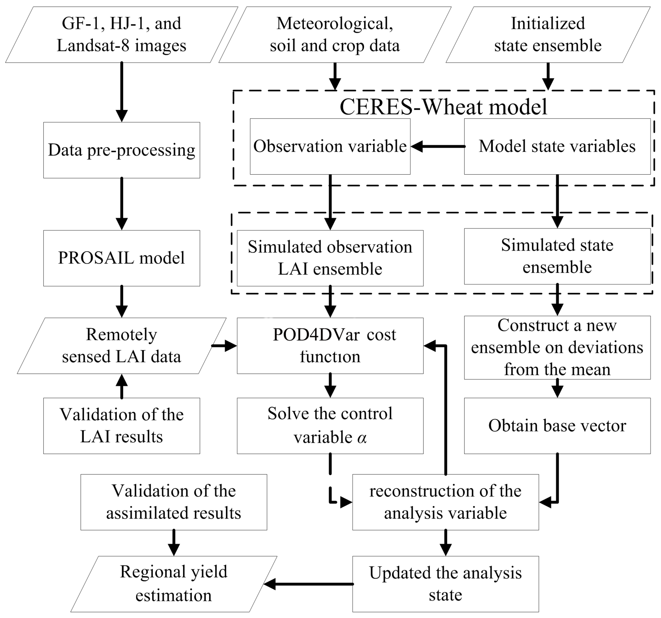
3.4. Ensemble-Based Four-Dimensional Variational Data Assimilation

The POD4DVar transforms an implicit optimization problem into an explicit functional minimization problem by merging the POD technique and the Monte Carlo method into the traditional 4DVar [81]. The basic idea is that a four-dimensional ensemble is firstly obtained from the forecast ensembles using the Monte Carlo method. Then, the POD is used to approximate the four-dimensional ensemble using a set of the orthogonal base vectors, which could capture the spatial structure of the state and temporal evolution. After the model states are represented by a truncated expansion of the base vectors, the control variables in the cost function appear explicit so that the optimal simulation results could be obtained, and the tangent linear or adjoint model is no longer required [9,81].

Compared to the PF strategy, the POD4DVar is a non-recursive process in which all observations at multiple times are used to solve all “analyses” in an assimilation process. In this study, the POD4DVar was also used to assimilate the observed LAI into the CERES-Wheat model to estimate the winter wheat yield. The whole calculation process mainly includes the stages of constructing a new ensemble matrix on deviations from the mean, computing the POD modes matrix and reconstruction of the analysis variable, reconstructing the cost function, solving the control variable and state estimation. The detailed process was reported previously [9], and the flowchart is shown in Figure 3.

The same as the PF assimilation strategy, the plant leaf area and observational LAI are both considered as state variables and observation vectors, respectively, in the POD4DVar data assimilation process.

4. Results

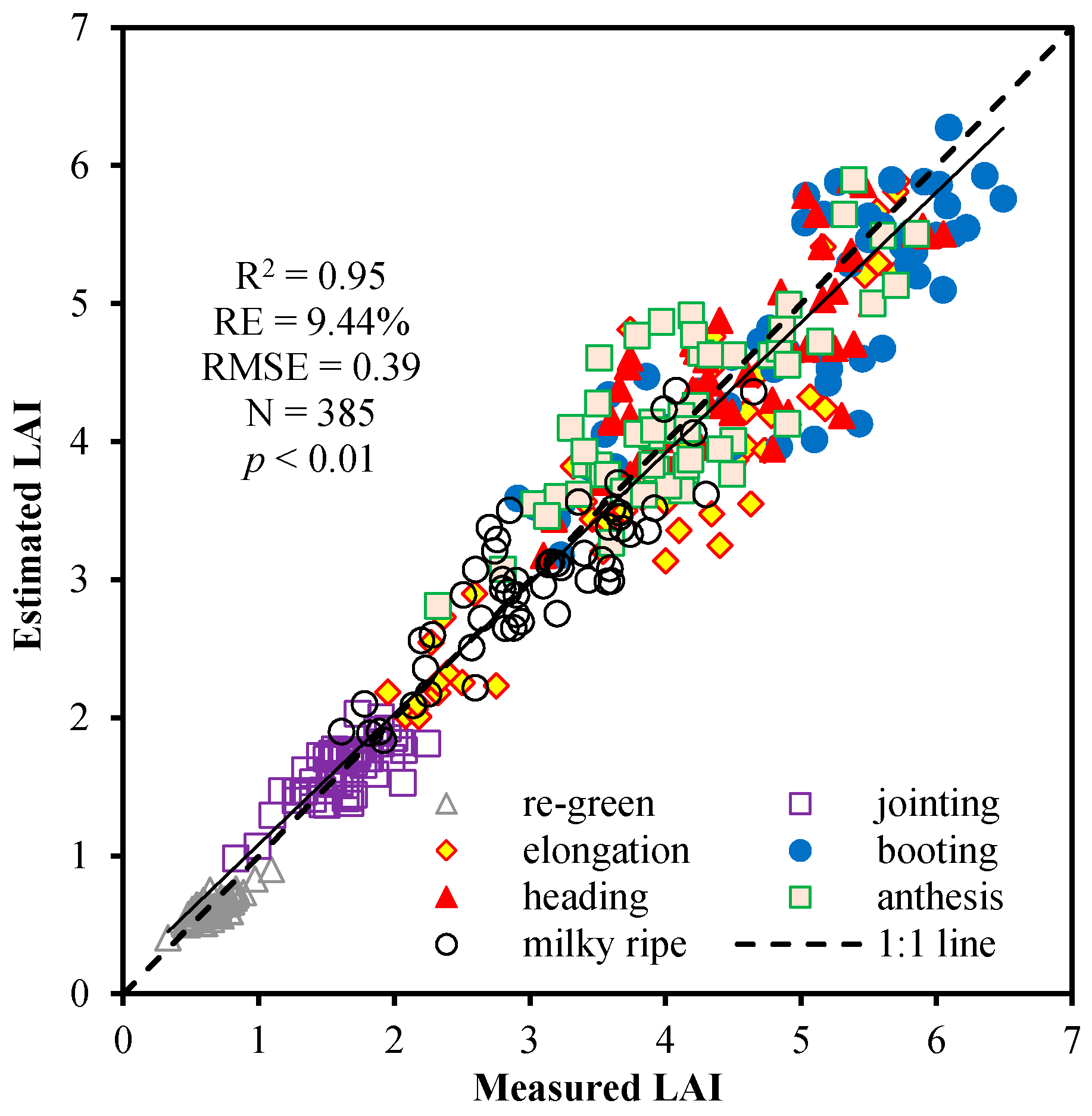
4.1. Remotely-Sensed LAI Estimates

In this study, 16 images with a high overall quality between green-up and maturity in 2014 were acquired, and the inversion of LAI was carried out by the PROSAIL radiation model based on the LUT method. The LAI estimated maps were validated by comparing the LAI values measured in the 55 sample plots at seven phenological stages with the corresponding values estimated from the LAI maps. The results (

Table 5. Validation of winter wheat LAI at different phenological stages. RE, relative error.

	Green-up	Jointing	Elongation	Booting	Heading	Anthesis	Maturity
R2	0.66	0.54	0.83	0.74	0.64	0.66	0.78
RE (%)	12.18	9.33	9.74	8.97	7.75	9.37	8.77
RMSE	0.09	0.19	0.46	0.51	0.45	0.44	0.32

) showed that the estimated LAI at seven key phenological stages have high correlation with the measured LAI, with an R² value of >0.54. A t-test [82] was used to determine whether the fitting curves between the measured LAI and the estimated LAI were the best fit. The linear regression formulas all passed the t-test (p < 0.05) with no significant difference. The accuracies of the estimated LAI were also all high, with the relative error (RE) values of <12.18% and the RMSE values of <0.51. Additionally, the total accuracy of the estimated LAI is also high, with an RE value of 9.44% and an RMSE value of 0.39 (Figure 4). The validation results showed that the remotely-sensed LAI maps accurately represented the LAI values during the given time periods and the temporal changes in LAI and could be employed in crop model data assimilations.

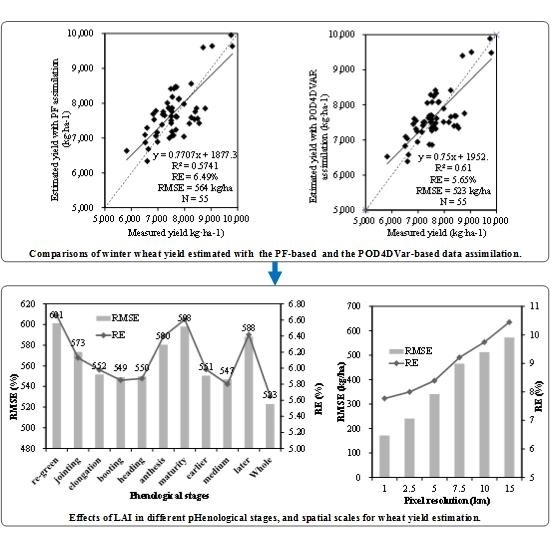
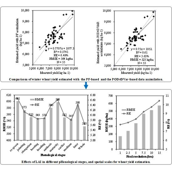
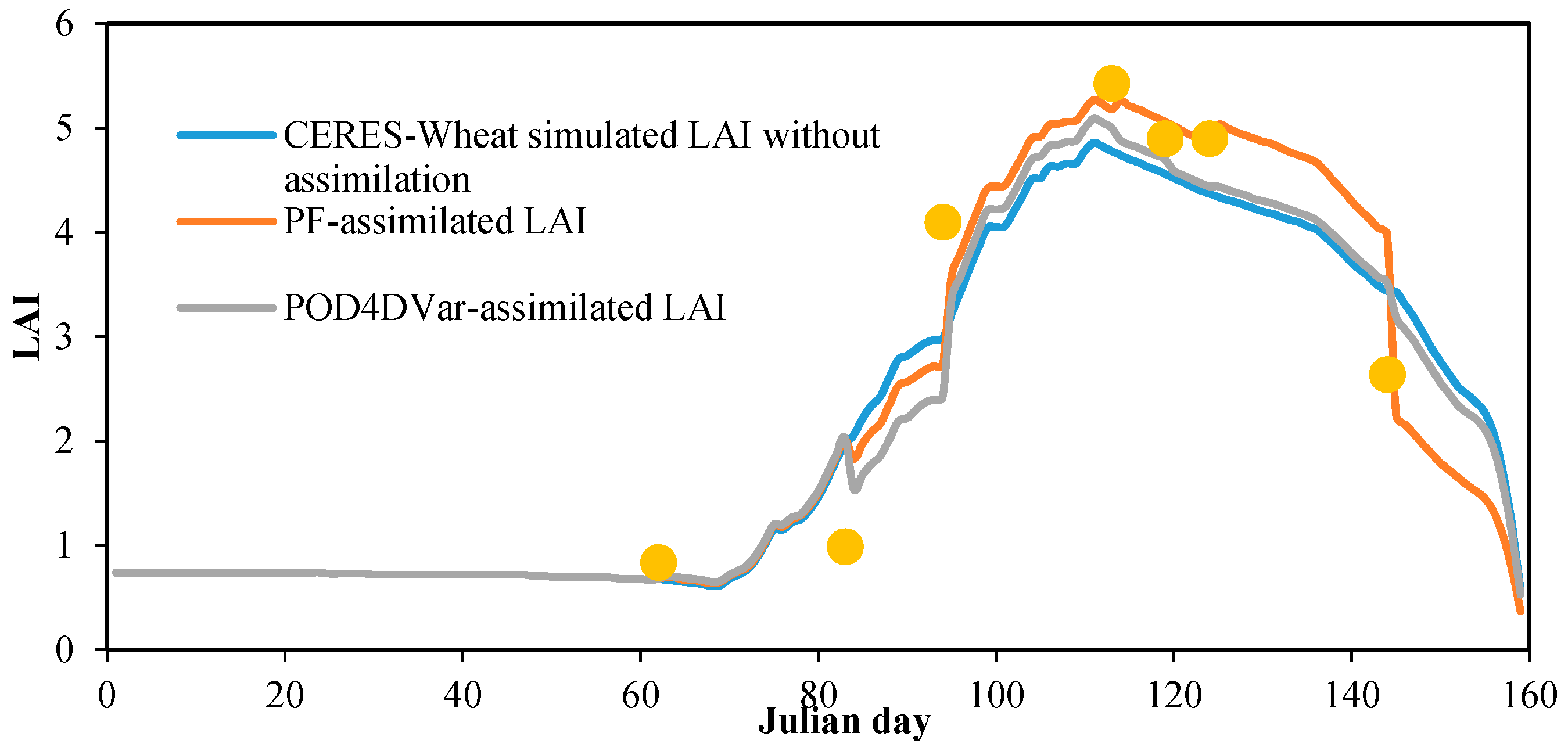
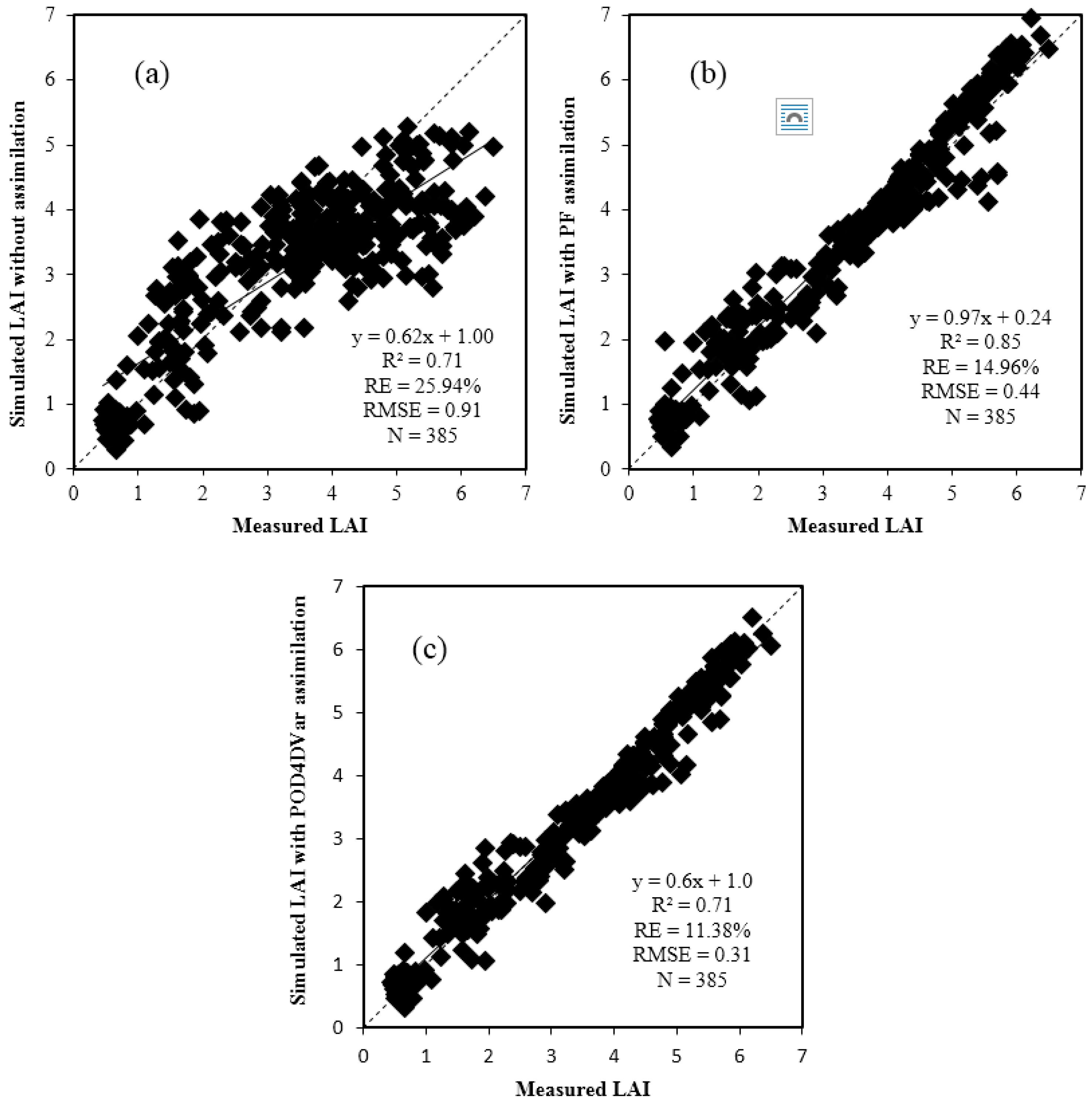
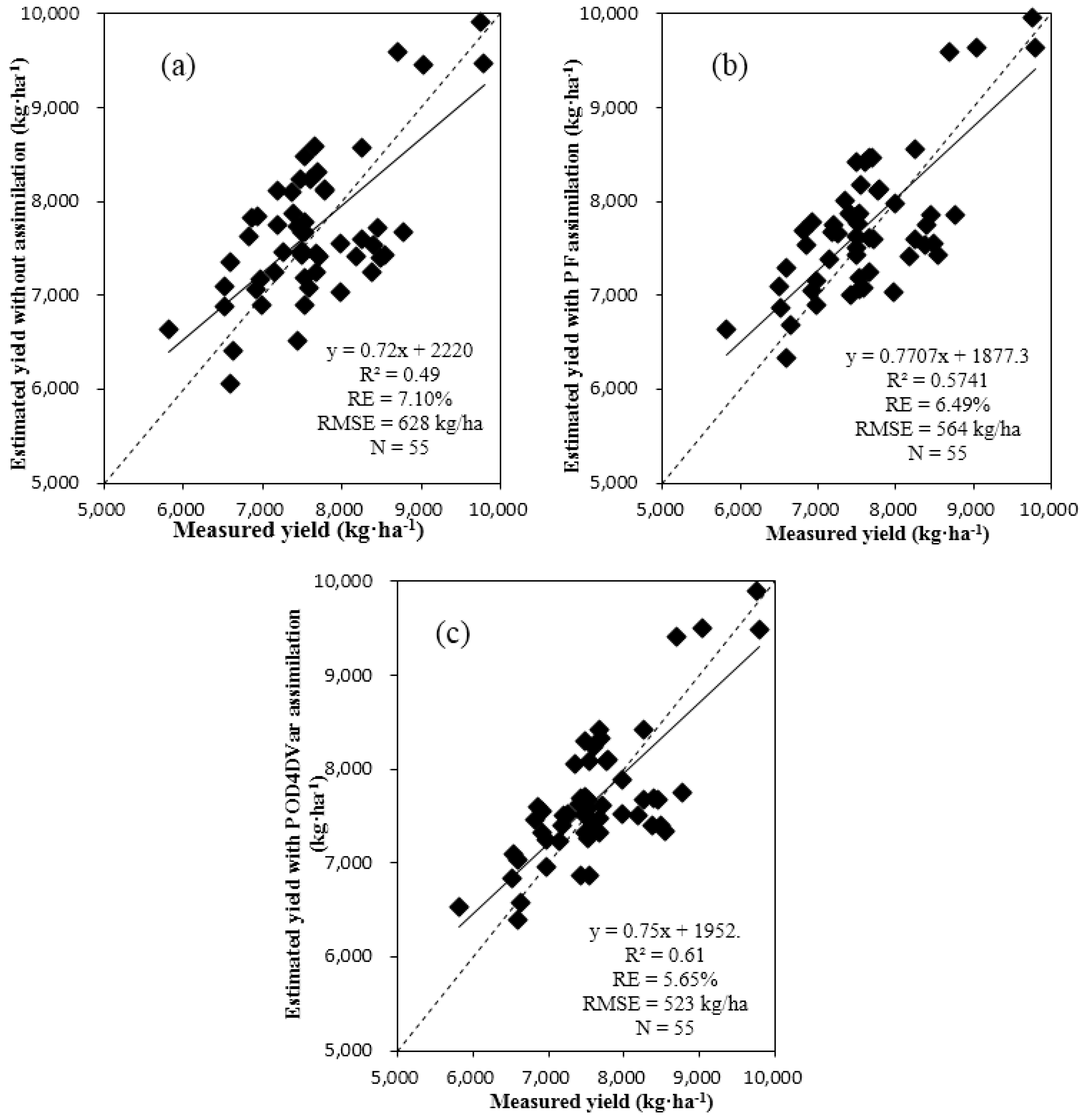
4.2. Comparison of Crop Yield Estimates Based on Data Assimilation at the Field Scale

To explore the performances and uncertainty between different assimilation algorithms, two assimilation algorithms (PF and POD4DVar) were applied to the crop model data assimilation at the field scale, respectively. To compare the performance of the PF-based and POD4DVar-based data assimilation strategies, both methods were performed with the same simulation conditions, including model inputs, initial conditions and seven assimilating LAIs measured at each field plot. Additionally, the ensemble/particle size was set to 100 to accurately and stably estimate the crop yield [10,16,40,66], and the standard deviation of the observation (10% of the observational LAI) was calculated from the measured observations.

We firstly compared the three assimilated LAI trajectories with PF-based, POD4DVar-based and without assimilation at the field scale (Figure 5). The results show that the simulated LAI trajectories with the two assimilation strategies are closer to the observations than the simulation curve without assimilation. Then, we compared the simulated LAIs with measured LAI (Figure 6). The accuracy is relatively low with an R² of 0.71, an RMSE of 0.91 and an RE of 25.94% between the simulated LAI without assimilation and observations at the field scale. Compared to the simulated LAI process without data assimilation, it was evident that the assimilation strategy dramatically improved the LAI estimates. The improved LAI estimates were observed with an R² of 0.85, an RMSE of 0.44 and an RE of 14.96% for the PF-based assimilation strategy and with an R² of 0.71, an RMSE of 0.31 and an RE of 11.38% for the POD4DVar-based assimilation strategy. The results show that the POD4DVar-based assimilation strategy provides a better promising approach for improving the wheat LAI estimation.

Consequently, the yield estimates were dramatically improved because of the optimization of the LAI simulation process (Figure 7). Compared with the simulated yields with no assimilation (Figure 6a), the estimated yields with the PF-based assimilation better predicted the measured yields, with an R² of 0.57, an RMSE of 564 kg·ha⁻¹ and an RE of 6.49% (Figure 7b). Comparing the three processes, the estimated yields with the POD4DVar-based assimilation predicted the measured yields better, with an R² of 0.61, an RMSE of 523 kg·ha⁻¹ and an RE of 5.65% (Figure 7c). Furthermore, less computing time was required for the POD4DVar-based assimilation (4.41 s over an assimilation window) than the PF-based assimilation (35.69 s). A comparison of the yield estimate experiments without assimilation and assimilation with the two algorithms indicated that the employed crop model data assimilation provides a promising approach for improving the wheat yield estimation. The experimental results also support the practical feasibility of the POD4DVar-based crop model data assimilation, especially in terms of yield estimation accuracy and computational efficiency. Thus, the subsequent simulations all used the POD4DVar-based assimilation strategy.

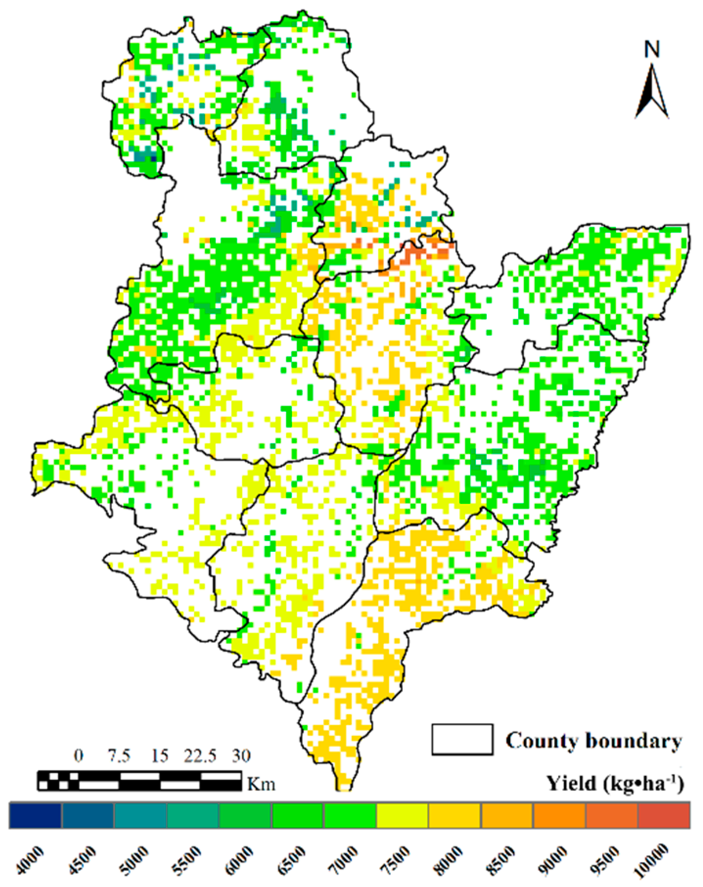
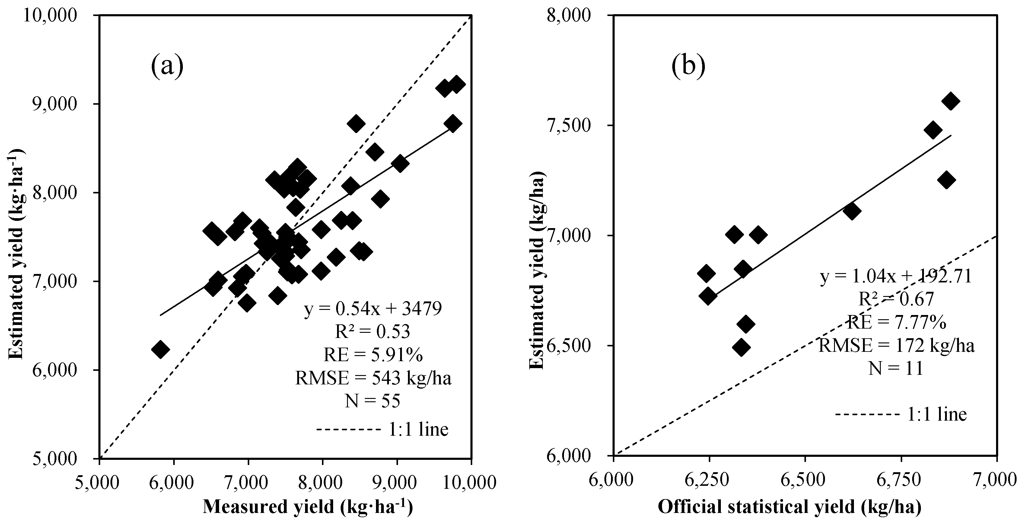
4.3. Assimilation of Remotely-Sensed LAI at the Regional Scale

Remotely-sensed LAI are an important information source for describing the growth of regional winter wheat. In addition, these data are the main source of information for correcting the crop model simulation process. To map the regional winter wheat yield, 16 remotely-sensed LAI data from the crop growing season were averaged to allow scaling up to a 1-km spatial resolution and then assimilated into the CERES-Wheat model using the POD4DVar-based strategy. The yield map showed that the yield per unit area generally decreased from south to north of Hengshui (Figure 8). The average yield over the study region was 6996 kg·ha⁻¹; the yield range was from 4480–9558 kg·ha⁻¹. The maximum productive capacity was observed in Gucheng County (7611 kg·ha⁻¹), followed by Wuyi (7479 kg·ha⁻¹) and Wuqiang (7253 kg·ha⁻¹) counties. The minimum yield was 6493 kg·ha⁻¹ in Raoyang County.

The accuracy of the crop yield estimation was evaluated at the pixel and county scales. The estimated yields of the 55 pixels closely agreed with the actual yields of the field plots with an R² of 0.53, an RMSE of 543 kg·ha⁻¹ and an RE of 5.91% (Figure 9a). Then, the estimated yields with a 1-km spatial resolution were aggregated at the county level so that the results could be validated using regional official yield statistics, which are compiled at the county level. The statistical mean yields of 11 counties showed that the R² was 0.67, the RMSE was 172 kg·ha⁻¹ and the RE was 7.77% (Figure 9b). The results also showed that the estimated yields are generally slightly higher than the official statistical yields. The reasons are mainly because most of the field plots’ observational yields (five of seven plots) in the agricultural experiment station were slightly higher than the official statistical yields, which led to the higher simulated yields and assimilated yields after the calibration of the crop model. However, on the whole, the estimated statistical mean yields own small deviations with the official statistical yields, and the accuracy is relatively high. These results suggest that the POD4DVar-based assimilation of remotely-sensed LAI significantly improved the simulation of yields with CERES-Wheat at the pixel and county scales.

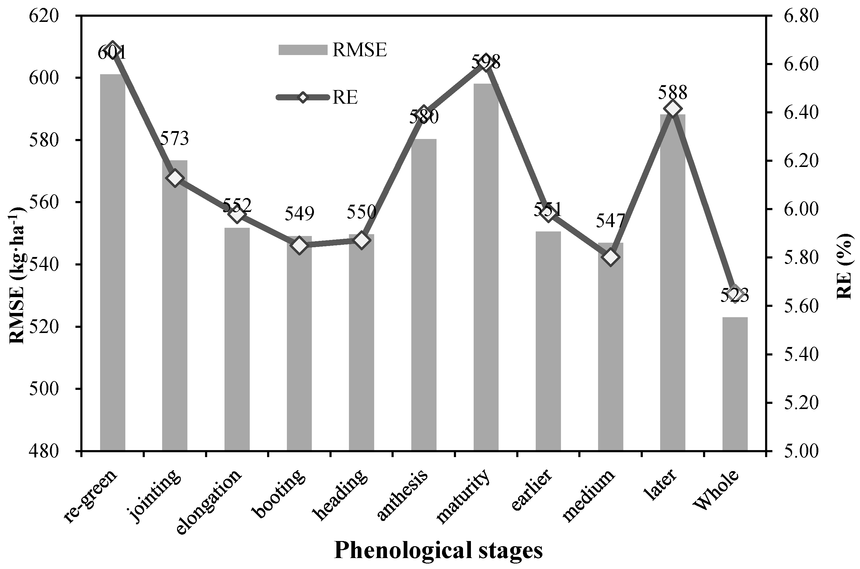
4.4. Effects of LAI in Different Phenological Stages for Wheat Yield Estimation at the Field Scale

To analyze the impacts of LAI in different phenological stages, the measured LAI during the seven individual phenological stages, earlier stage (green-up and jointing), medium stage (booting, heading and flowering), later stage (anthesis and maturity) and whole period (all seven phenological stages) in the 55 sample plots at the field scale were all simulated. Wheat yield estimation experiments with different phenological stages (Figure 10) showed that the LAIs at booting and heading both played the most critical roles with RE of 5.85% and 5.87%, RMSE of 549 kg·ha⁻¹ and 550 kg·ha⁻¹ and both R² of 0.59, when considering only individual stages. Canopy LAI values of wheat at these two stages are at a maximum and closely related to the final yields. In addition to the above two stages, the order is followed by the LAI during the elongation, jointing, anthesis, maturity and green-up stages. The least importance of the LAI values during the maturity and green-up stages is because they do not adequately represent the temporal variability of the LAI trajectory. Crop yield estimation experiments with four different combining stages (Figure 10) showed that the worst performance was the assimilation of observations at the later stage, with the RE of 6.42%, RMSE of 588 kg·ha⁻¹ and R² of 0.54. In contrast, the LAI during the medium stages showed better performances, with the RE of 5.80%, normalized RMSE of 547 kg·ha⁻¹ and R² of 0.59. Overall, assimilating the measured LAI with whole phenological stages achieved the best accuracy compared with any single phenological stage or the earlier, medium or later stages. Thus, it is important to obtain observations between jointing and anthesis as much as possible (particularly for the elongation, booting and heading stage) to improve the accuracies of the crop yield estimation when observing scarcity.

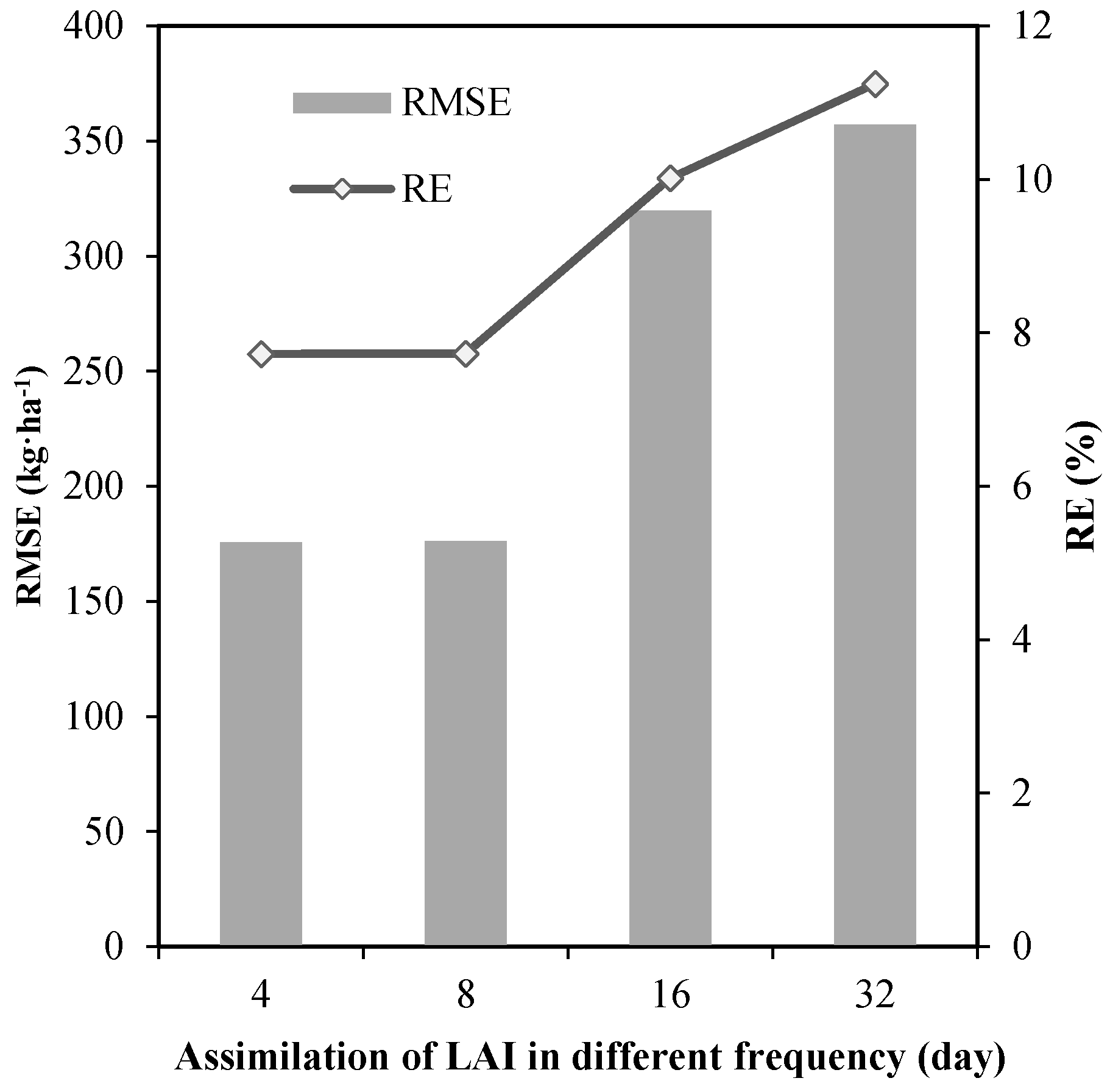
4.5. Effects of LAI in Different Temporal Frequencies for Wheat Yield Estimation at the Regional Scale

In consideration of LAI in different phenological periods affecting the assimilating yield, the LAI at different temporal frequencies also affects the simulated results. To analyze the impacts of the temporal frequency of LAI for yield estimates, the smooth remotely-sensed LAI trajectory from green-up to maturity after S-G filtering was divided into four different frequencies (four days with 24 images, eight days with 12 images, 16 days with six images and 32 days with three images) to assess the accuracies of the yield estimates, respectively. The assimilation of LAI during the growing season could effectively correct the simulated trajectory of LAI in CERES-Wheat, and the simulated LAI curve would move gradually closer to the real LAI curve during the growing season. Hence, modest increases in the frequency of assimilating observations may improve yield estimations. The results (Figure 11) showed that the accuracies of the assimilated yields tended to gradually drop as the frequency of assimilating LAI decreased from 32 days to four, the RE increased from 7.72%–11.24% and the RMSE increased from the 176–357 kg·ha⁻¹, especially for the frequency of 16 days and 32 days, whereas the computation time that is required for the yield estimation of a given pixel decreased. The estimated yield from the assimilating frequency of four days to eight days seems to have a similar accuracy, with an RE of 7.723%–7.726% and an RMSE of 175 kg·ha⁻¹–176 kg·ha⁻¹. Therefore, selecting a reasonable frequency of assimilating LAI (e.g., eight days) could improve the computational efficiency and accuracy of regional crop yield estimations.

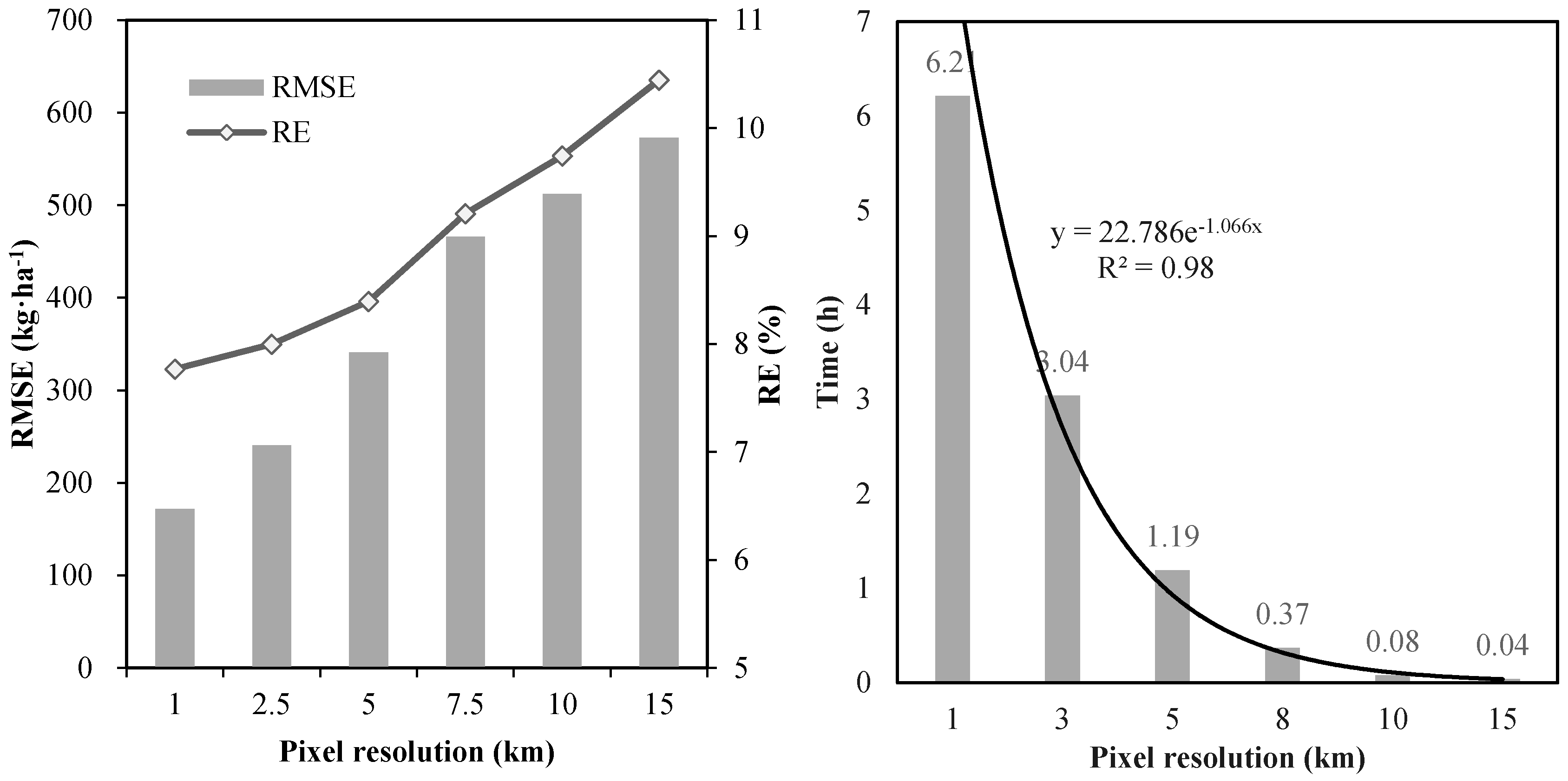
4.6. Effects of LAI at Different Spatial Scales for Wheat Yield Estimation

Regional crop yield estimates mainly rely on remotely-sensed LAIs during the crop growth season. In addition to the effects of LAI in different temporal scales (containing the phenological stages and temporal frequency), the spatial scale of LAI also affects the accuracy of regional yield estimations. For example, coarser pixels with abundant mixed landscape patterns usually result in greater spatial scale errors of LAI values obtained from more heterogeneous surface, which increase the errors of regional crop yield estimates. In addition, the abundant and detailed information that is supplied by remote sensing data with high spatio-temporal resolution is limited by high computational costs. To analyze the impacts of LAI at different spatial scales, six spatial scales of LAI (with pixel sizes of 1 km, 2.5 km, 5 km, 7.5 km, 10 km and 15 km) were aggregated based on the nearest neighbor algorithm by using the remotely-sensed LAI data and assimilated into a crop model using the POD4DVar-based strategy to estimate regional yield. The results (Figure 12) showed that the accuracies of the assimilated yields at the county scale tended to gradually decrease as the pixel resolution of assimilating LAI decreased from 1 km–15 km, the RE increased from 7.77%–10.45% and the RMSE increased from the 172–573 kg·ha⁻¹, respectively. In contrast, the computation time decreased from 6.21 h down to 0.04 h. Consequently, it is important to select a reasonable pixel size for remotely-sensed observations to compromise between the accuracy and efficiency of operational regional crop yield estimation systems.

5. Discussion

Crop growth models often oversimplify actual crop growth conditions. Some uncertainty is introduced by the model’s structure, the model assumed, observation errors and meteorological parameters, resulting in a biased simulation of the true growth process. Without altering the crop models’ structure, the uncertainties of the crop model can be reduced using the assimilation of observational LAI during the crop growing season. To obtain better estimates of regional crop information, a series of remotely-sensed LAIs during the crop growing season must also be accurately estimated [6]. Unfortunately, current remote sensing LAIs have several shortcomings in their temporal and spatial resolutions due to the limits of the revisit circle, the cloud coverage and/or mixed pixels, which may result in poor performance of the assimilation process. To reduce these uncertainties in observation errors, we retrieved LAIs using the PROSAIL model with multiple sensors’ optical data (i.e., Landsat OLI, HJ-1 and GF-1) to improve accuracy and increase the effective temporal resolution of remotely-sensed LAI. On the other hand, we constructed two strategies (PF and POD4DVar) to assimilate the observed LAI directly into the CERES-Wheat model and compared the performances of these two strategies at the field scale. It was found that the employed POD4DVar-based assimilation strategy is the better approach for improving the wheat modeled LAI and yield estimation. Then, based on the POD4DVar-based assimilation framework, we analyzed the performance of crop model assimilation of LAI at different temporal scales (phenological stages and temporal frequencies) and spatial scales.

Compared with traditional EnKF-based strategy and re-recalibration strategies (e.g., SCE-UA [5]), the PF-based strategy can sample particles and update particle weights according to any distribution function and is able to express the model estimation as a recursive process that avoids the higher dimensions of control variables and a high computational burden [22]. In this study, the resampling and reperturbation of the resampled particles were used to avoid the particle degeneracy and lack of particle diversity under the constraints of the model by using fewer particles. However, the particles would increase exponentially in order for the posterior mean from the particle filter to have an expected error smaller than either the prior or the observations [83]. This study provides new progress and challenges that will be addressed in our future work. Compared with the EnKF-based strategy, the POD4DVar-based strategy can perfectly solve the issues in non-Gaussian dynamic distributions and nonlinear models, which avoids the greater dimensions of control variables and computational costs, so as to obtain higher accuracy and lower computational costs than EnKF [9]. By merging the Monte Carlo and POD into the 4DVar method, the POD4DVar-based strategy retains the main advantages of the traditional 4DVar (i.e., dynamic constraint and assimilation of multiple time observations) [40] and need not maintain and update the adjoint or tangent linear models of the forecast models [9]. Compared with the PF-based strategies, our results indicated that the POD4DVar-based assimilation strategy results in better performance and higher computational efficiency of the assimilation process and is the better approach for improving the wheat modeled LAI and yield estimation. However, the uncertainty of the ensemble size and the initial perturbation fields on the assimilated results were not shown in this study and will be addressed in our future work.

Unfortunately, few studies have focused on the application of PF-based and POD4DVar-based assimilation strategies to yield estimations. In this study, the uncertain effects of the LAI in different temporal scales (phenological stages and temporal frequencies) and spatial scales were given greater emphasis. The optimal yield estimates may be highly dependent on the reasonable spatio-temporal resolution of assimilating LAI. Observations between jointing and anthesis stages (particularly for the elongation, booting and heading stage) play important roles in improving the accuracies of the crop yield estimation when observing scarcity. This finding is similar to the observations of Huang et al. [6], in which the MODIS-LAI model was assimilated into the WOFOST (World Food Studies) model. In addition to this, LAI with a high frequency and spatial resolution significantly improved the accuracy of crop yield estimations, although the increased computing time may be problematic for regional applications. This finding is similar to the observations of Jiang et al. [22], in which the HJ-LAI model was assimilated into the CERES-Wheat model. Thus, the use of the POD4DVar-based strategy to assimilate LAI with moderate spatial resolution (e.g., 1 km), phenological stages between jointing and anthesis stages and an assimilation temporal frequency of eight days appears to be a promising assimilation approach with reasonable spatio-temporal scale to achieve a tradeoff between accuracy and effectiveness in regional wheat estimate applications.

When remotely-sensed LAIs are used to replace the value of a model-simulated state variable in a data assimilation system, one assumes that the remotely-sensed LAIs are free of error or assumes that the level of data error is acceptable to be propagated within the simulated system [53]. To reduce the errors, the remotely-sensed LAIs were retrieved using the PROSAIL model from multiple sensors’ optical data (i.e., Landsat OLI, HJ-1 and GF-1) and accurately obtained the results. However, the uncertainty effects of the remotely-sensed observations’ errors on assimilated yield estimates based on the method of error perturbation are not shown in this study and will be addressed in our future work.

In this study, the independent assimilation of LAI was a preferred method for optimally estimating the crop yields from plots with relatively wet soils that were extensively irrigated during the crop growth season. This finding is similar to the observations of Nearing et al. and Ines et al. [53,68], in which the LAI and soil moisture were assimilated into the decision support system for the agro-technology transfer-cropping system (DSSAT-CSM) model. This finding is also similar to the observations of Huang et al. [5], in which the MODIS LAI and ET products were assimilated into the WOFOST model. Thus, assimilating LAI, evapotranspiration (ET) and/or soil moisture represents another important area of research that will be investigated further, especially in arid and semi-arid areas.

Although the POD4DVar-based assimilation method achieved good results in 2014, the capabilities about the method presented in prediction mode with other years were not shown in this study. An extension of multiple years to validate the assimilation method and determine how well it accounts for the inter-annual variability in crop yield prediction is needed and will be addressed in our future work.

6. Conclusions

In this study, the data assimilation methods of PF and POD4DVar were used to improve the performance of the CERES-Wheat model for yield estimates. Compared with traditional assimilations of crop models, we mainly focus on the uncertainties of wheat yield estimates due to different assimilation strategies and multi-source errors, such as the remotely-sensed LAIs, assimilation strategies, temporal scales (phenological stages and temporal frequencies) and the spatial scale.

The experimental results showed that the accuracy and temporal resolution of remotely-sensed LAI can be improved and increased by using the PROSAIL model with multi-sensors’ optical data (i.e., Landsat OLI, HJ-1 and GF-1). The inversed LAIs could be employed in crop model data assimilations. Compared with the crop model without assimilation, the crop model with the PF-based and POD4DVar-based strategies provides significantly better regional crop yield estimates, especially for the POD4DVar-based strategy, which resulted in greater performance of the assimilation model. Although the best yield estimates were obtained when all of the observed LAIs during the crop growing season were assimilated into the crop model, an acceptable estimate of crop yield could also be achieved by assimilating fewer observations between the jointing and anthesis periods of the crop growth season. Good performance was observed when the frequency of the assimilation observations increased from four to 32 days, and the assimilation temporal frequency of eight days also appears to be a reasonable tradeoff between the accuracy and effectiveness in regional wheat estimate applications. In contrast, the accuracy of the regional crop yield estimates generally decreased as the spatial resolution of the LAI decreased from 15 km down to 1 km. Conversely, the computation times were lower for the assimilation of observations with lower spatial resolution. Thus, the use of the POD4DVar-based strategy to assimilate LAI with moderate spatial resolution (e.g., 1 km), phenological stages between jointing and anthesis stages and assimilation of the temporal frequency of eight days appears to be a reasonable tradeoff between accuracy and effectiveness in regional wheat estimates.

References

1. Rae, A.; Pardey, P. Global food security-introduction. Aust. J. Agric. Resour. Econ. 2014, 58, 499–503. [Google Scholar] [CrossRef]
2. Lipper, L.; Thornton, P.; Campbell, B.M.; Baedeker, T.; Braimoh, A.; Bwalya, M.; Caron, P.; Cattaneo, A.; Garrity, D.; Henry, K. Climate-smart agriculture for food security. Nat. Clim. Chang. 2014. [Google Scholar] [CrossRef]
3. Zhao, Y.; Chen, S.; Shen, S. Assimilating remote sensing information with crop model using ensemble kalman filter for improving LAI monitoring and yield estimation. Ecol. Model. 2013, 270, 30–42. [Google Scholar] [CrossRef]
4. Li, Y.; Zhou, Q.; Zhou, J.; Zhang, G.; Chen, C.; Wang, J. Assimilating remote sensing information into a coupled hydrology-crop growth model to estimate regional maize yield in arid regions. Ecol. Model. 2014, 291, 15–27. [Google Scholar] [CrossRef]
5. Huang, J.; Ma, H.; Su, W.; Zhang, X.; Huang, Y.; Fan, J.; Wu, W. Jointly assimilating MODIS LAI and ET products into the swap model for winter wheat yield estimation. IEEE J. Sel. Top. Appl. Earth Obs. Remote Sens. 2015, 8, 4060–4071. [Google Scholar] [CrossRef]
6. Huang, J.; Tian, L.; Liang, S.; Ma, H.; Becker-Reshef, I.; Huang, Y.; Su, W.; Zhang, X.; Zhu, D.; Wu, W. Improving winter wheat yield estimation by assimilation of the leaf area index from Landsat Tm and MODIS data into the WOFOST model. Agric. For. Meteorol. 2015, 204, 106–121. [Google Scholar] [CrossRef]
7. Fang, H.; Liang, S.; Hoogenboom, G. Integration of MODIS LAI and vegetation index products with the CSM–CERES–Maize model for corn yield estimation. Int. J. Remote Sens. 2011, 32, 1039–1065. [Google Scholar] [CrossRef]
8. Doraiswamy, P.C.; Moulin, S.; Cook, P.W.; Stern, A. Crop yield assessment from remote sensing. Photogramm. Eng. Remote Sens. 2003, 69, 665–674. [Google Scholar] [CrossRef]
9. Jiang, Z.; Chen, Z.; Chen, J.; Ren, J.; Li, Z.; Sun, L. The estimation of regional crop yield using ensemble-based four-dimensional variational data assimilation. Remote Sens. 2014, 6, 2664–2681. [Google Scholar] [CrossRef]
10. De Wit, A.J.W.; van Diepen, C.A. Crop model data assimilation with the ensemble kalman filter for improving regional crop yield forecasts. Agric. For. Meteorol. 2007, 146, 38–56. [Google Scholar] [CrossRef]
11. Srivastava, A.K.; Gaiser, T. Simulating biomass accumulation and yield of yam (Dioscorea alata) in the upper ouémé basin (Benin Republic)-I. Compilation of physiological parameters and calibration at the field scale. Field Crop. Res. 2010, 116, 23–29. [Google Scholar] [CrossRef]
12. Van der Velde, M.; Wriedt, G.; Bouraoui, F. Estimating irrigation use and effects on maize yield during the 2003 heatwave in France. Agric. Ecosyst. Environ. 2010, 135, 90–97. [Google Scholar] [CrossRef]
13. Rinaldi, M.; de Luca, D. Application of EPIC model to assess climate change impact on sorghum in southern Italy. Ital. J. Agron. 2012. [Google Scholar] [CrossRef]
14. Confalonieri, R.; Acutis, M.; Bellocchi, G.; Donatelli, M. Multi-metric evaluation of the models warm, cropsyst, and WOFOST for rice. Ecol. Model. 2009, 220, 1395–1410. [Google Scholar] [CrossRef]
15. De Wit, A.J.W.; Boogaard, H.L.; van Diepen, C.A. Spatial resolution of precipitation and radiation: The effect on regional crop yield forecasts. Agric. For. Meteorol. 2005, 135, 156–168. [Google Scholar] [CrossRef]
16. Wang, J.; Li, X.; Lu, L.; Fang, F. Estimating near future regional corn yields by integrating multi-source observations into a crop growth model. Eur. J. Agron. 2013, 49, 126–140. [Google Scholar] [CrossRef]
17. De Wit, A.; Duveiller, G.; Defourny, P. Estimating regional winter wheat yield with WOFOST through the assimilation of green area index retrieved from MODIS observations. Agric. For. Meteorol. 2012, 164, 39–52. [Google Scholar] [CrossRef]
18. Vazifedoust, M.; van Dam, J.C.; Bastiaanssen, W.G.M.; Feddes, R.A. Assimilation of satellite data into agrohydrological models to improve crop yield forecasts. Int. J. Remote Sens. 2009, 30, 2523–2545. [Google Scholar] [CrossRef]
19. Launay, M.; Guerif, M. Assimilating remote sensing data into a crop model to improve predictive performance for spatial applications. Agric. Ecosyst. Environ. 2005, 111, 321–339. [Google Scholar] [CrossRef]
20. Luo, Y.; Ogle, K.; Tucker, C.; Fei, S.; Gao, C.; LaDeau, S.; Clark, J.S.; Schimel, D.S. Ecological forecasting and data assimilation in a data-rich era. Ecol. Appl. 2011, 21, 1429–1442. [Google Scholar] [CrossRef] [PubMed]
21. Ma, G.; Huang, J.; Wu, W.; Fan, J.; Zou, J.; Wu, S. Assimilation of MODIS-LAI into the WOFOST model for forecasting regional winter wheat yield. Math. Comput. Model. 2013, 58, 634–643. [Google Scholar] [CrossRef]
22. Jiang, Z.W.; Chen, Z.X.; Chen, J.; Liu, J.; Ren, J.Q.; Li, Z.N.; Sun, L.; Li, H. Application of crop model data assimilation with a particle filter for estimating regional winter wheat yields. IEEE J. Sel. Top. Appl. Earth Obs. Remote Sens. 2014, 7, 4422–4431. [Google Scholar] [CrossRef]
23. Cheng, Z.; Meng, J.; Wang, Y. Improving spring maize yield estimation at field scale by assimilating time-series HJ-1 CCD data into the WOFOST model using a new method with fast algorithms. Remote Sens. 2016, 8, 303. [Google Scholar] [CrossRef]
24. Dong, T.; Liu, J.; Qian, B.; Zhao, T.; Jing, Q.; Geng, X.; Wang, J.; Huffman, T.; Shang, J. Estimating winter wheat biomass by assimilating leaf area index derived from fusion of Landsat-8 and MODIS data. Int. J. Appl. Earth Obs. 2016, 49, 63–74. [Google Scholar] [CrossRef]
25. Huang, J.; Sedano, F.; Huang, Y.; Ma, H.; Li, X.; Liang, S.; Tian, L.; Zhang, X.; Fan, J.; Wu, W. Assimilating a synthetic Kalman filter leaf area index series into the WOFOST model to estimate regional winter wheat yield. Agric. For. Meteorol. 2016, 216, 188–202. [Google Scholar] [CrossRef]
26. Ines, A.V.M.; Hansen, J.W.; Robertson, A.W. Enhancing the utility of daily GCM rainfall for crop yield prediction. Int. J. Climatol. 2011, 31, 2168–2182. [Google Scholar] [CrossRef]
27. Dorigo, W.A.; Zurita-Milla, R.; de Wit, A.J.W.; Brazile, J.; Singh, R.; Schaepman, M.E. A review on reflective remote sensing and data assimilation techniques for enhanced agroecosystem modeling. Int. J. Appl. Earth Obs. 2007, 9, 165–193. [Google Scholar] [CrossRef]
28. Ma, Y.; Wang, S.; Zhang, L.; Hou, Y.; Zhuang, L.; He, Y.; Wang, F. Monitoring winter wheat growth in North China by combining a crop model and remote sensing data. Int. J. Appl. Earth Obs. 2008, 10, 426–437. [Google Scholar]
29. Powell, M.J.D. An efficient method for finding the minimum of a function of several variables without calculating derivatives. Comput. J. 1964, 7, 155–162. [Google Scholar] [CrossRef]
30. Fang, H.; Liang, S.; Hoogenboom, G.; Teasdale, J.; Cavigelli, M. Corn-yield estimation through assimilation of remotely sensed data into the CSM-CERES-Maize model. Int. J. Remote Sens. 2008, 29, 3011–3032. [Google Scholar] [CrossRef]
31. Kirkpatrick, S.; Gelatt, C.D.; Vecchi, M.P. Optimization by simulated annealing. Science 1983, 220, 671–680. [Google Scholar] [CrossRef] [PubMed]
32. Duan, Q.Y.; Gupta, V.K.; Sorooshian, S. Shuffled complex evolution approach for effective and efficient global minimization. J. Optim. Theory Appl. 1993, 76, 501–521. [Google Scholar] [CrossRef]
33. Dente, L.; Satalino, G.; Mattia, F.; Rinaldi, M. Assimilation of leaf area index derived from ASAR and MERIS data into CERES-Wheat model to map wheat yield. Remote Sens. Environ. 2008, 112, 1395–1407. [Google Scholar] [CrossRef]
34. Sabater, J.M.; Rüdiger, C.; Calvet, J.C.; Fritz, N.; Jarlan, L.; Kerr, Y. Joint assimilation of surface soil moisture and LAI observations into a land surface model. Agric. For. Meteorol. 2008, 148, 1362–1373. [Google Scholar] [CrossRef] [Green Version]
35. Ma, H.; Huang, J.; Zhu, D.; Liu, J.; Su, W.; Zhang, C.; Fan, J. Estimating regional winter wheat yield by assimilation of time series of HJ-1 CCD NDVI into WOFOST–ACRM model with ensemble kalman filter. Math. Comput. Model. 2013, 58, 759–770. [Google Scholar] [CrossRef]
36. Li, R.; Li, C.; Dong, Y.; LIU, F.; Wang, J.; Yang, X.; Pan, Y. Assimilation of remote sensing and crop model for LAI estimation based on ensemble kaiman filter. Agric. Sci. Chin. 2011, 10, 1595–1602. [Google Scholar] [CrossRef]
37. Evensen, G. The ensemble kalman filter: Theoretical formulation and practical implementation. Ocean Dyn. 2003, 53, 343–367. [Google Scholar] [CrossRef]
38. Li, Z.; Zhao, L.; Fu, Z. Estimating net radiation flux in the tibetan plateau by assimilating MODIS LST products with an ensemble kalman filter and particle filter. Int. J. Appl. Earth Obs. 2012, 19, 1–11. [Google Scholar] [CrossRef]
39. Arulampalam, M.S.; Maskell, S.; Gordon, N.; Clapp, T. A tutorial on particle filters for online nonlinear/non-Gaussian Bayesian tracking. IEEE Trans. Signal Proc. 2002, 50, 174–188. [Google Scholar] [CrossRef]
40. Moore, A.M.; Arango, H.G.; Broquet, G.; Powell, B.S.; Weaver, A.T.; Zavala-Garay, J. The regional ocean modeling system (ROMS) 4-dimensional variational data assimilation systems part I—System overview and formulation. Prog. Oceanogr. 2011, 91, 34–49. [Google Scholar] [CrossRef]
41. Curnel, Y.; de Wit, A.J.W.; Duveiller, G.; Defourny, P. Potential performances of remotely sensed LAI assimilation in WOFOST model based on an OSS experiment. Agric. For. Meteorol. 2011, 151, 1843–1855. [Google Scholar] [CrossRef]
42. Tian, X.; Xie, Z.; Sun, Q. A pod-based ensemble four-dimensional variational assimilation method. Tellus A 2011, 63, 805–816. [Google Scholar] [CrossRef]
43. Tian, X.; Xie, Z.; Dai, A.; Shi, C.; Jia, B.; Chen, F.; Yang, K. A dual-pass variational data assimilation framework for estimating soil moisture profiles from AMSR-E microwave brightness temperature. J. Geophys. Res. 2009. [Google Scholar] [CrossRef]
44. Moradkhani, H.; De Chant, C.M.; Sorooshian, S. Evolution of ensemble data assimilation for uncertainty quantification using the particle filter-markov chain Monte Carlo method. Water Resour. Res. 2012. [Google Scholar] [CrossRef]
45. Leisenring, M.; Moradkhani, H. Analyzing the uncertainty of suspended sediment load prediction using sequential data assimilation. J. Hydrol. 2012, 468, 268–282. [Google Scholar] [CrossRef]
46. Nagarajan, K.; Judge, J.; Graham, W.D.; Monsivais-Huertero, A. Particle filter-based assimilation algorithms for improved estimation of root-zone soil moisture under dynamic vegetation conditions. Adv. Water Resour. 2011, 34, 433–447. [Google Scholar] [CrossRef]
47. Leisenring, M.; Moradkhani, H. Snow water equivalent prediction using Bayesian data assimilation methods. Stoch. Environ. Res. Risk Assess. 2011, 25, 253–270. [Google Scholar] [CrossRef]
48. Montzka, C.; Moradkhani, H.; Weihermueller, L.; Franssen, H.H.; Canty, M.; Vereecken, H. Hydraulic parameter estimation by remotely-sensed top soil moisture observations with the particle filter. J. Hydrol. 2011, 399, 410–421. [Google Scholar] [CrossRef]
49. Chen, Y.; Cournède, P.H. Data assimilation to reduce uncertainty of crop model prediction with convolution particle filtering. Ecol. Model. 2014, 290, 165–177. [Google Scholar] [CrossRef]
50. Cao, Y.; Zhu, J.; Navon, I.M.; Luo, Z. A reduced-order approach to four-dimensional variational data assimilation using proper orthogonal decomposition. Int. J. Numer. Methods Fluids 2007, 53, 1571–1583. [Google Scholar] [CrossRef]
51. Tian, X.; Xie, Z. Effects of sample density on the assimilation performance of an explicit four-dimensional variational data assimilation method. Sci. China Earth Sci. 2009, 52, 1849–1856. [Google Scholar] [CrossRef]
52. Hansen, J.W.; Challinor, A.; Ines, A.; Wheeler, T.; Moron, V. Translating climate forecasts into agricultural terms: Advances and challenges. Clim. Res. 2007, 33, 27–41. [Google Scholar] [CrossRef]
53. Ines, A.V.M.; Das, N.N.; Hansen, J.W.; Njoku, E.G. Assimilation of remotely sensed soil moisture and vegetation with a crop simulation model for maize yield prediction. Remote Sens. Environ. 2013, 138, 149–164. [Google Scholar] [CrossRef]
54. Claverie, M.; Demarez, V.; Duchemin, B.; Hagolle, O.; Ducrot, D.; Marais-Sicre, C.; Dejoux, J.; Huc, M.; Keravec, P.; Béziat, P.; et al. Maize and sunflower biomass estimation in southwest france using high spatial and temporal resolution remote sensing data. Remote Sens. Environ. 2012, 124, 844–857. [Google Scholar] [CrossRef] [Green Version]
55. Plummer, S.; Arino, O.; Ranera, F.; Tansey, K.; Chen, J.; Dedieu, G.; Eva, H.; Piccolini, I.; Leigh, R.; Borstlap, G.; et al. The globcarbon initiative—Global biophysical products for terrestrial carbon studies. In Proceedings of the 2007 IEEE International Geoscience and Remote Sensing Symposium, Barcelona, Spain, 23–28 July 2007.
56. Champeaux, J.L.; Masson, V.; Chauvin, R. Ecoclimap: A global database of land surface parameters at 1 km resolution. Meteorol. Appl. 2005, 12, 29–32. [Google Scholar] [CrossRef]
57. Yang, W.; Tan, B.; Huang, D.; Rautiainen, M.; Shabanov, N.V.; Wang, Y.; Privette, J.L.; Huemmrich, K.F.; Fensholt, R.; Sandholt, I.; et al. MODIS leaf area index products: from validation to algorithm improvement. IEEE Trans. Geosci. Remote. 2006, 44, 1885–1898. [Google Scholar] [CrossRef]
58. Jones, J.W.; Hoogenboom, G.; Porter, C.H.; Boote, K.J.; Batchelor, W.D.; Hunt, L.A.; Wilkens, P.W.; Singh, U.; Gijsman, A.J.; Ritchie, J.T. The DSSAT cropping system model. Eur. J. Agron. 2003, 18, 235–265. [Google Scholar] [CrossRef]
59. LI-COR Inc. LAI-2200 Plant Canopy Analyzer, Introduction Manual; LI-COR Inc.: Lincoln, NE, USA, 2010. [Google Scholar]
60. Shi, X.Z.; Yu, D.S.; Warner, E.D.; Sun, W.X.; Petersen, G.W.; Gong, Z.T.; Lin, H. Cross-reference system for translating between genetic soil classification of china and soil taxonomy. Soil Sci. Soc. Am. J. 2006, 70, 78–83. [Google Scholar] [CrossRef]
61. Shi, X.Z.; Yu, D.S.; Warner, E.D.; Pan, X.Z.; Petersen, G.W.; Gong, Z.G.; Weindorf, D.C. Soil database of 1:1,000,000 digital soil survey and reference system of the Chinese genetic soil classification system. Soil Surv. Horiz. 2004, 45, 129–136. [Google Scholar] [CrossRef]
62. Ding, D. Soil Species of Hebei Province; Hebei Science and Technology Press: Shijiazhuang, China, 1992. [Google Scholar]
63. Al-Sadah, F.H.; Ragab, F.M. Study of global daily solar radiation and its relation to sunshine duration in bahrain. Sol. Energy 1991, 47, 115–119. [Google Scholar] [CrossRef]
64. Allen, R.G.; Pereira, L.S.; Raes, D.; Smith, M. Crop Evapotranspiration: Guidelines for Computing Crop Water Requirements; FAO Irrigation and Drainage Paper No. 56; FAO: Rome, Italy, 1998. [Google Scholar]
65. Hutchinson, M.F. ANUSPLIN Version 4.37 User Guide. Available online: http://fennerschool.anu.edu.au/files/anusplin437.pdf (accessed on 18 July 2007).
66. Singh, A.K.; Tripathy, R.; Chopra, U.K. Evaluation of CERES-Wheat and CropSyst models for water-nitrogen interactions in wheat crop. Agric. Water Manag. 2008, 95, 776–786. [Google Scholar] [CrossRef]
67. Dettori, M.; Cesaraccio, C.; Motroni, A.; Spano, D.; Duce, P. Using CERES-Wheat to simulate durum wheat production and phenology in southern Sardinia, Italy. Field Crop. Res. 2011, 120, 179–188. [Google Scholar] [CrossRef]
68. Nearing, G.S.; Crow, W.T.; Thorp, K.R.; Moran, M.S.; Reichle, R.H.; Gupta, H.V. Assimilating remote sensing observations of leaf area index and soil moisture for wheat yield estimates: An observing system simulation experiment. Water Resour. Res. 2012, 48, 213–223. [Google Scholar] [CrossRef]
69. Saltelli, A.; Tarantola, S.; Chan, K. A quantitative model-independent method for global sensitivity analysis of model output. Technometrics 1999, 41, 39–56. [Google Scholar] [CrossRef]
70. Pasolli, L.; Asam, S.; Castelli, M.; Bruzzone, L.; Wohlfahrt, G.; Zebisch, M.; Notarnicola, C. Retrieval of leaf area index in mountain grasslands in the alps from MODIS satellite imagery. Remote Sens. Environ. 2015, 165, 159–174. [Google Scholar] [CrossRef]
71. Darvishzadeh, R.; Atzberger, C.; Skidmore, A.; Schlerf, M. Mapping grassland leaf area index with airborne hyperspectral imagery: A comparison study of statistical approaches and inversion of radiative transfer models. ISPRS J. Photogramm. 2011, 66, 894–906. [Google Scholar] [CrossRef]
72. Darvishzadeh, R.; Skidmore, A.; Schlerf, M.; Atzberger, C. Inversion of a radiative transfer model for estimating vegetation LAI and chlorophyll in a heterogeneous grassland. Remote Sens. Environ. 2008, 112, 2592–2604. [Google Scholar] [CrossRef]
73. Richter, K.; Atzberger, C.; Vuolo, F.; D’Urso, G. Evaluation of sentinel-2 spectral sampling for radiative transfer model based LAI estimation of wheat, sugar beet, and maize. IEEE J. Sel. Top. Appl. Earth Obs. Remote Sens. 2011, 4, 458–464. [Google Scholar] [CrossRef]
74. Nigam, R.; Bhattacharya, B.K.; Vyas, S.; Oza, M.P. Retrieval of wheat leaf area index from awifs multispectral data using canopy radiative transfer simulation. Int. J. Appl. Earth Obs. 2014, 32, 173–185. [Google Scholar] [CrossRef]
75. Duan, S.; Li, Z.; Wu, H.; Tang, B.; Ma, L.; Zhao, E.; Li, C. Inversion of the prosail model to estimate leaf area index of maize, potato, and sunflower fields from unmanned aerial vehicle hyperspectral data. Int. J. Appl. Earth Obs. 2014, 26, 12–20. [Google Scholar] [CrossRef]
76. Darvishzadeh, R.; Matkan, A.A.; Dashti Ahangar, A. Inversion of a radiative transfer model for estimation of rice canopy chlorophyll content using a lookup-table approach. IEEE J. Sel. Top. Appl. Earth Obs. Remote Sens. 2012, 5, 1222–1230. [Google Scholar] [CrossRef]
77. Dorigo, W.A. Improving the robustness of cotton status characterisation by radiative transfer model inversion of multi-angular chris/proba data. IEEE J. Sel. Top. Appl. Earth Obs. Remote Sens. 2012, 5, 18–29. [Google Scholar] [CrossRef]
78. Aplin, P. Image analysis, classification and change detection in remote sensing, with algorithms for envi/idl. Int. J. Geogr. Inf. Sci. 2009, 23, 129–130. [Google Scholar]
79. Savitzky, A.; Golay, M.J.E. Smoothing and differentiation of data by simplified least squares procedures. Anal. Chem. 1964, 36, 1627–1639. [Google Scholar] [CrossRef]
80. Li, H.; Chen, Z.; Wu, W.; Jiang, Z.; Liu, B.; Hasi, T. Crop model data assimilation with particle filter for yield prediction using leaf area index of different temporal scales. In Proceedings of the Fourth International Conference on Agro-Geoinformatics, Istanbul, Turkey, 20–24 July 2015.
81. Tian, X.; Xie, Z.; Dai, A. An ensemble-based explicit four-dimensional variational assimilation method. J. Geophys. Res. 2008, 113, 6089. [Google Scholar] [CrossRef]
82. Boneau, C.A. The effects of violations of assumptions underlying the t test. Psychol. Bull. 1960, 57, 49–64. [Google Scholar] [CrossRef] [PubMed]
83. Snyder, C.; Bengtsson, T.; Bickel, P.; Anderson, J. Obstacles to high-dimensional particle filtering. Mon. Weather Rev. 2008, 136, 4629–4640. [Google Scholar] [CrossRef]
Figure 1. Location of the study area, experimental and meteorological stations, sample plots and the spatial distribution of winter wheat in 2014.
Remotesensing 09 00190 g001
Figure 2. The flowchart of CERES-Wheat model data assimilation with PF.
Remotesensing 09 00190 g002
Figure 3. Flowchart of the proper orthogonal decomposition-based ensemble four-dimensional variational (POD4DVar) strategy with the CERES-Wheat crop model.
Remotesensing 09 00190 g003
Figure 4. Comparison of the observed and inverted LAIs during critical growth periods of winter wheat.
Remotesensing 09 00190 g004
Figure 5. Comparison of the LAI curves with PF-based assimilation, POD4DVar-based assimilation and without assimilation at the field scale.
Remotesensing 09 00190 g005
Figure 6. Comparisons of winter wheat LAI with (a) no data assimilation; (b) the PF-based data assimilation and (c) the POD4DVar-based data assimilation.
Remotesensing 09 00190 g006
Figure 7. Comparisons of winter wheat yield estimated by the CERES-Wheat model with (a) no data assimilation, (b) the PF-based data assimilation and (c) the POD4DVar-based data assimilation.
Remotesensing 09 00190 g007
Figure 8. Distribution of winter wheat yield estimates with a 1-km scale using POD4DVar.
Remotesensing 09 00190 g008
Figure 9. Comparisons between the measured and estimated yields at the pixel (a) and county scales (b).
Remotesensing 09 00190 g009
Figure 10. Accuracy of the estimated wheat yield using LAI from different phenological stages or combinations of these stages compared with the measured yield at the field scale.
Remotesensing 09 00190 g010
Figure 11. Accuracy of estimated wheat yield using LAI from a different temporal frequency compared with the official statistical yields at the regional scale.
Remotesensing 09 00190 g011
Figure 12. Accuracy and computation time of estimated wheat yield using LAI from a different spatial scales compared with the official statistical yields.
Remotesensing 09 00190 g012