Towards a Universal Hyperspectral Index to Assess Chlorophyll Content in Deciduous Forests

Abstract

The reflectance properties of leaves are influenced by diverse biochemical components including chlorophyll, one of the key indicators related to plant photosynthesis and plant stress. Although a number of hyperspectral indices have been proposed for quantifying leaf chlorophyll concentrations, their applications are largely restricted to where they were developed and can hardly provide satisfactory results in other cases. In this study, universally applicable hyperspectral indices calculated from both original and first-order derivative spectra were identified for quantifying leaf chlorophyll concentrations in deciduous forests. Using the main criteria of the ratio of performance to deviation (RPD) and the widely applicable information criterion (WAIC), new hyperspectral indices were proposed for quantifying chlorophyll concentrations in four independent datasets. The results revealed that the normalized derivative difference between the green peak (520–540 nm) and the end of the red edge (720–740 nm) were effective. The normalized difference type of index using reflectance derivatives at 522 and 728 nm, dND (522, 728), was the most effective index for quantifying chlorophyll concentrations, with an R² of 0.807 and a lowest root mean square error of 8.67 μg/cm², n = 816. This index was also validated based on a simulated dataset generated from the model of PROpriétés SPECTrales Version 5 (PROSPECT 5). Its applicability for assessing chlorophyll content in various deciduous forests was hence demonstrated. We foresee its wide application in the future.

1. Introduction

Chlorophyll content is one of the most important biochemical materials, closely related to the photosynthetic process and with protective activity against a variety of degenerative diseases [1]. Changes in the chlorophyll content of leaves may thus indicate effects of disease and nutritional and environmental stresses [2]. Increasing attention to global issues over the recent past requires quick evaluation of chlorophyll content on a large scale in order to assess various biogeochemical processes. Although there are several instruments available to provide in situ measurements of chlorophyll content (e.g., soil plant analysis development, SPAD, chlorophyll meter), remote sensing (especially hyperspectral remote sensing) remains as one of the most attractive options for large-scale chlorophyll content monitoring, if not the only attractive option, based on which many easy-to-apply vegetation indices calculated from hyperspectral reflectance have been developed [3].

There are two main approaches for quantifying leaf chlorophyll concentrations using hyperspectral remote sensing; the first is through the numerical inversion of radiative transfer models, and another is through the application of hyperspectral indices. Compared with the inversion approach, the application of hyperspectral indices is convenient and may be potentially applied for large-scale monitoring if general ones are developed.

It is widely known that chlorophyll strongly absorbs light at blue (400–500 nm) and red (600–700 nm) spectra and does not include light in the green and orange (500–600 nm) spectra [4]. The differences in reflectance between healthy and stressed vegetation can be detected in changes to the green peak and the red edge [5]. As a result, most hyperspectral indices for assessing chlorophyll content generally use the wavelength domain ranging from 400 to 860 nm, on either original reflectance or derivative spectra. They may also be categorized roughly into two types: one is original or derivative value-based indices, and the other is spectral feature based, which generally uses spectral patterns, mainly based on the properties of the red-edge such as the point of maximum slope [6,7,8,9] or a sum of derivative values [10,11].

Although numerous vegetation indices for estimating chlorophyll content have been proposed, no consensus has ever been reached, since most indices are only applicable to where and when they are developed. Our previous study on deciduous forests revealed that most indices may be categorized into two groups: shade-oriented or sunlit leaf-oriented indices, which performed poorly with the other leaf type [12]. Deciduous forests generally have two distinctive leaf groups with different biochemical, biophysical and physiological properties, and we found no hyperspectral index in a total of 86 published indices for chlorophyll content applicable to both leaf types and different deciduous species in the cold temperate climate zone.

The main aim of this study is therefore oriented towards developing general applicable indices for quantifying chlorophyll concentrations in deciduous forests. This is based on two distinctive datasets with synchronous measurements of leaf chlorophyll and reflectance. One dataset was obtained from natural beech (Fagus creanata) leaves (sunshade and sunlit) in Mount Naeba, (Niigata Prefecture, Japan) and the other with a total of 29 different deciduous species in Nakagawane (Shizuoka Prefecture, Japan). In addition, two independent online datasets including 23 different deciduous species from the Joint Research Centre Leaf Optical Properties Experiment (LOPEX) [13] and 23 different deciduous species from ANGERS [14], which is the dataset measured in 2003 at INRA in Angers (France), were used for validations. Furthermore, an additional evaluation was also conducted using a simulated dataset generated from the popular leaf scale radiative transfer model PROpriétés SPECTrales Version 5 (PROSPECT 5) [14], which was calibrated using randomly selected samples for the four independent datasets, to examine the robustness of the proposed indices.

Furthermore, hyperspectral data are currently available from Hyperion onboard Earth Observing-1 (EO-1), with 10-nm spectral information from 350 to 2500 nm [15], and several other missions, such as the Hyper-spectral Imager SUIte (HISUI) composed of 185 spectral bands in the visible and near-infrared to shortwave infrared region at 30-m spatial resolution [16,17]. Thus, the robustness of hyperspectral indices related to downscaled spectral resolution should also be evaluated in order to apply the hyperspectral data obtained from the sensors onboard satellites as opposed to spectroscopy data.

In order to develop a robustness index for quantifying chlorophyll concentration, we applied the ratio of performance to deviation (RPD), which is an indicator for assessing the goodness of fit and expressed as a ratio of standard error in prediction to the standard deviation of the samples [18], as the primary criterion to determine the optimal index. Based on the RPD, all indices were categorized into three ranks, namely category A: RPD > 2.0, category B: RPD 1.4–2.0 and category C: RPD < 1.4. Those evaluated as C were generally not applicable. In this study, only those indices categorized as ‘B’ or above for each of four independent datasets were selected. However, a selection solely based on RPD sometimes may lead to a wrong decision [19]. As thus, the widely applicable information criterion (WAIC) [20] was adopted to make the final selection of the best indices.

2. Materials and Methods

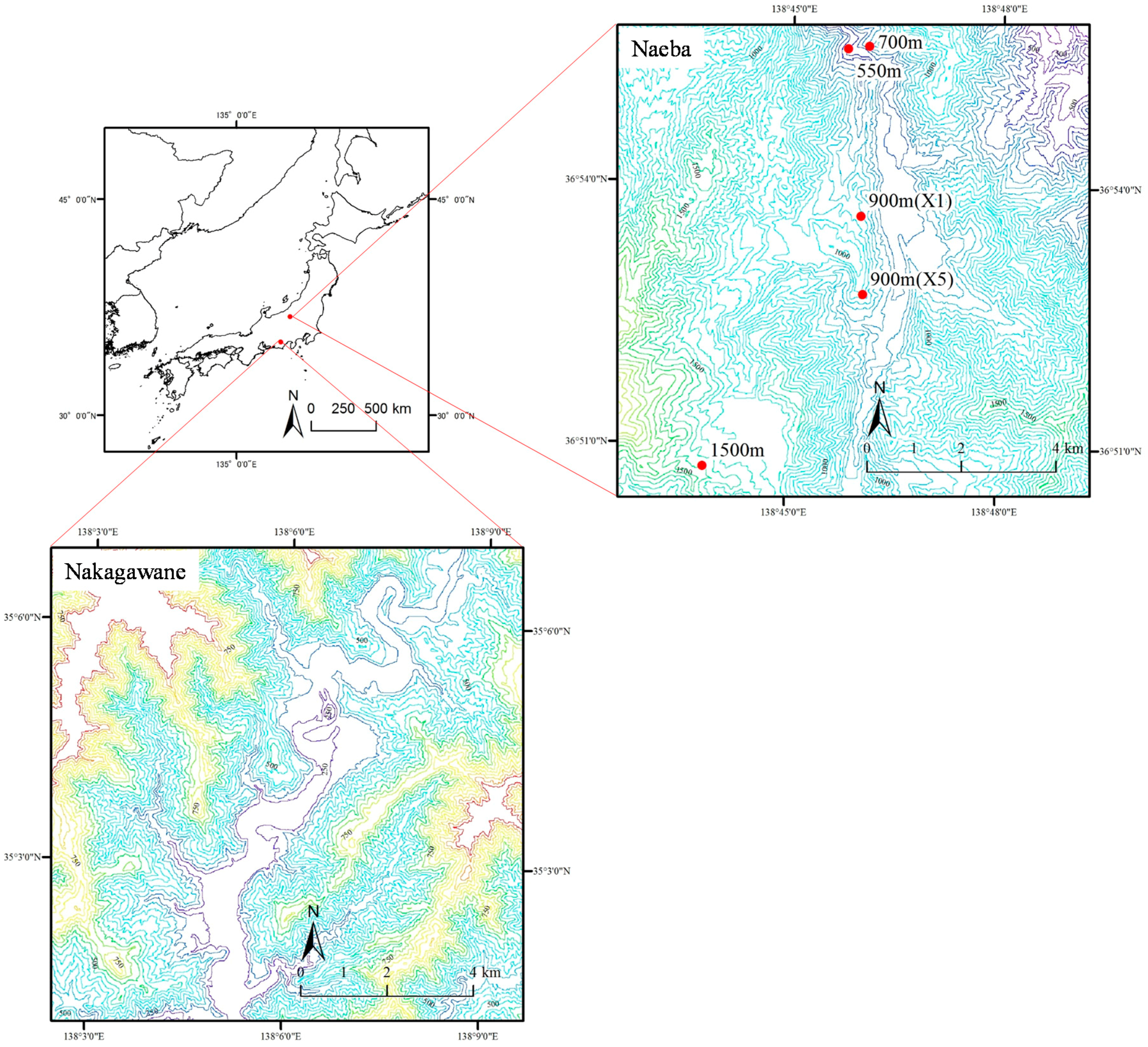
2.1. Study Sites

In this study, two independent field datasets acquired respectively from two typical alpine cold-temperate climate areas (see Figure 1 for locations) were used. The first site is located in the Naeba Mountains, Niigata (Japan; latitude 36°50′N and longitude 138°41′E, adjacent to the Sea of Japan), where both sunlit and shaded leaves of beech (Fagus crenata, the dominant species at this site) were collected. This region has high precipitation of approximately 2000 mm·year⁻¹ and is characterized by heavy snowfall. The annual mean air temperature is between 10.1 and 12.7 °C [21]. It has also been an important site for SpecNet (Spectral Network), which is an international network of cooperating investigators and sites linking optical measurements with flux sampling [22]. Various leaf properties, including various types of pigments, nitrogen, maximum rate of carboxylation (V_cmax), equivalent water thickness (EWT), leaf thickness, leaf mass area (LMA) and leaf anatomy, have been measured continuously since 2000 [23]. In this study, beech leaves sampled at 900 m X1, 700 m and 550 m were used.

The second site is located in Nakagawane, one of the university forests of Shizuoka University (Japan; lat. 35°04′N and long. 138°06′E, facing the Pacific Ocean coast), where 29 deciduous species (Acer argutum, Acer capillipes, Acer micranthum, Acer mono, Acer nipponicum, Acer rufinerve, Acer sieboldianum, Carpinus japonica, Clethra barbinervis, Enkianthus campanulatus, Euptelea polyandra, Ilex macropoda, Kalopanax septemlobus, Lindera praecox, Lindera umbellata, Magnolia obovata, Pourthiaea villosa var. zollingeri, Prunus buergeriana, Prunus maximowiczii, Pterostyrax hispida, Quercus crispula, Rhododendron dilatatum, Rhododendron quinquefolium, Styrax japonica, Styrax shiraianus, Symplocos coreana, Tilia japonica, Viburnum furcatum and Viburnum wrightii) were collected. The site is at an elevation of between 390 and 1560 m and is characterized by high precipitation of approximately 2500 mm·year⁻¹. The annual mean air temperature is ca. 16 °C [21].

It has been reported that the forests expanded from each refugia along the Sea of Japan or the Pacific Ocean [24] after the last glacial maximum, and the vegetation histories were different between the area adjacent to the Sea of Japan and that adjacent to the Pacific Ocean [25]. The two sites hence have different vegetation histories and different climate characteristics and should be useful to evaluate hyperspectral indices.

2.2. Measurements and Field Datasets

The detached branch method [26,27] was applied for leaf sampling. Leaf sampling for this study was conducted from June 2007 to August 2013 in Mt. Naeba but only in the summer of 2014 at the Nakagawane site. Spectral reflectance measurements and biochemical analysis of leaf samples were carried out within three days after sampling. Before that, all samples were kept in a dark environment. A FieldSpec spectrometer (Analytical Spectral Devices Inc., Boulder, CO, USA) adopted with a leaf clip in order to obtain reflectance data with low error, which is related to the effects of broadband illumination, was used for the reflectance measurements. Leaf discs for chlorophyll concentration measurements were punched after leaf reflectance measurements and then frozen in liquid nitrogen before they were analyzed using dual-beam scanning ultraviolet-visible spectrophotometers (Ultrospec 3300 pro, Amersham Biosciences, Piscataway, NJ, USA). Arnon’s method [28] was applied to calculate chlorophyll content after absorption.

In addition, those data of broadleaf species containing two online datasets compiled from two experimental campaigns were used for further validation: one is LOPEX [13], which includes the measurements of 23 broadleaf species, namely Acer pseudoplatanus, Alnus glutinosa, Betula pendula, Castanea sativa, Corylus avellana, Fagus sylvatica, Ficus carica, Fraxinus excelsior, Hedera helix, Juglans regia, Morus alba, Morus nigra, Populus tremula, Populus x canadensis, Prunus armeniaca, Prunus serotina, Quercus pubescens, Quercus rubra, Robinia pseudoacacia, Salix alba, Tilia platyphyllos, Ulmus glabra and Vitis vinifera; the other is called ANGERS [14], which contains the measurements of 23 broadleaf species including Acer negundo, Acer pseudoplatanus, Alnus glutinosa, Calicarpa bodinieri, Castanea sativa, Cercis siliquastrum, Cornus alba, Corylus maxima, Cotinus coggygria, Hydrangea macrophylla, Liquidambar styraciflua, Liriodendron tulipifera, Parthenocissus tricuspidata, Populus alba, Quercus palustris, Rhus typhina, Robinia pseudoacacia, Salix atrocinerea, Syringa vulgaris, Tilia tomentosa, Viburnum plicatum, Vitis vinifera and Weigela florida.

As in LOPEX, five repetitions of the spectral measurement were conducted for each physical and biological measurement [13], their averaged reflectance values were hence adopted for further analysis in this study.

2.3. Simulated Dataset

To further evaluate the robustness of the indices, a simulated dataset generated from PROSPECT-5 was used in this study. This version was expressed as a function of leaf structure index (N), leaf chlorophyll content, carotenoid content, leaf water content (EWT, g/cm²) and leaf mass area (LMA, g/m²) and simulated leaf spectral reflectance and transmittance from 400 to 2500 nm with an interval of 1 nm. Before applying it to generate the reflectance dataset, the coefficients were calibrated according to the calibration algorithm of Feret et al. [14]. The simulation was conducted using these statistics (total chlorophyll content, carotenoid content, EWT, LMA, and N) and followed the procedure proposed by Pavan et al. [29].

2.4. Development of New Indices

Most published indices are expressed as reflectance or a first-order derivative at a given wavelength (R) [30,31,32], wavelength difference (D) [33,34], simple ratio (SR) [2,31,35,36,37,38,39,40,41,42,43,44,45,46,47,48,49], normalized difference (ND) [35,36,50,51,52] or double differences (DDn) [52,53]. Inverse reflectance differences (ID) such as the anthocyanin reflectance index (ARI) or carotenoid reflectance index (CRI) [54,55] have been proposed as well. Thus, six common types of indices based on either original reflectance or derivative spectra, as follows, were screened in this study:

$$\mathrm{R}\left({\lambda }_1\right)=R_{{\lambda }_1}$$

(1)

$$\mathrm{D}\left({\lambda }_1,{\lambda }_2\right)=R_{{\lambda }_1}-R_{{\lambda }_2}$$

(2)

$$\mathrm{SR}\left({\lambda }_1,{\lambda }_2\right)=R_{{\lambda }_1}/R_{{\lambda }_2}$$

(3)

$$\mathrm{ND}\left({\lambda }_1,{\lambda }_2\right)=(R_{{\lambda }_1}-R_{{\lambda }_2})/(R_{{\lambda }_1}+R_{{\lambda }_2})$$

(4)

$$\mathrm{DDn}\left({\lambda }_1,\Delta \mathsf{\lambda }\right)=2R_{{\lambda }_1}-R_{{\lambda }_1-\Delta \lambda }-R_{{\lambda }_1+\Delta \lambda }$$

(5)

$$\mathrm{ID}\left({\lambda }_1,{\lambda }_2\right)=1/R_{{\lambda }_1}-1/R_{{\lambda }_2}$$

(6)

and

$$\mathrm{dR}\left({\lambda }_1\right)=d{R}_{{\lambda }_1}$$

(7)

$$\mathrm{dD}\left({\lambda }_1,{\lambda }_2\right)=d{R}_{{\lambda }_1}-d{R}_{{\lambda }_2}$$

(8)

$$\mathrm{dSR}\left({\lambda }_1,{\lambda }_2\right)=d{R}_{{\lambda }_1}/d{R}_{{\lambda }_2}$$

(9)

$$\mathrm{dND}\left({\lambda }_1,{\lambda }_2\right)=(d{R}_{{\lambda }_1}-d{R}_{{\lambda }_2})/(d{R}_{{\lambda }_1}+d{R}_{{\lambda }_2})$$

(10)

$$\mathrm{dDDn}\left({\lambda }_1,\Delta \mathsf{\lambda }\right)=2d{R}_{{\lambda }_1}-d{R}_{{\lambda }_1-\Delta \lambda }-d{R}_{{\lambda }_1+\Delta \lambda }$$

(11)

$$\mathrm{dID}\left({\lambda }_1,{\lambda }_2\right)=1/d{R}_{{\lambda }_1}-1/d{R}_{{\lambda }_2}$$

(12)

where R is reflectance, dR is first-order derivative spectra and the suffixes (λ₁ or λ₂) are wavelength (nm). In the entire wavelength domain ranging from 400 to 2500 nm, these indices were evaluated by regression analysis with chlorophyll concentrations.

2.5. Statistical Criteria

The premier criterion of the ratio of performance to deviation (RPD), an indicator for assessing the goodness of fit and expressed as a ratio of the standard error in prediction to the standard deviation of the samples [18], was calculated from

$$\mathrm{RPD}=\mathrm{Sd}/\mathrm{SEP}$$

(13)

where SEP is standard error of prediction and Sd is standard deviation of the chlorophyll content.

The indices were then assigned to categories A, B and C accordingly, for which category A (RPD > 2.0), category B (1.4 ≤ RPD ≤ 2.0) and category C (RPD < 1.4) were defined [56]. It has been claimed that category B can be improved by using different calibration strategies, but properties in category C may not be reliably predicted [56]. Next, those indices ranked ‘B’ or better for the datasets from Naeba and Nakagawane were extracted, and their robustness was evaluated using the datasets from LOPEX and ANGERS, as well as the simulated dataset generated from a calibrated version of PROSPECT 5 covering the entire range of chlorophyll content in the four independent datasets.

The final selection of the best indices was based on the widely applicable information criterion (WAIC) [20], which is asymptotically equivalent to the leave-one-out cross-validation in Bayes estimation and is defined by

$$\mathrm{WAIC}=T_n+\raisebox{1ex}{$V_n$}\!\left/ \!\raisebox{-1ex}{$n$}\right.$$

(14)

where n is the number of training samples, T_n is the training loss, and V_n is the functional variance. These parameters are defined with posterior distribution on parameter w (E_w[]), the probability distribution ($p\left(X_i|w\right)$) and the predictive distribution defined by the model ($p^{*}\left(X_i|w\right)$).

$$T_n=-\frac{1}{n}{\displaystyle \sum }_{i=1}^n\log p^{*}\left(X_i|w\right)$$

(15)

$$V_n={\displaystyle \sum }_{i=1}^n\left\{E_w\left[{\left(\log p\left(X_i|w\right)\right)}^2\right]-E_w{\left[\log p\left(X_i|w\right)\right]}^2\right\}$$

(16)

Besides WAIC, the root mean square errors (RMSE) and the coefficient of determination (R²) were also calculated for assessment.

3. Results

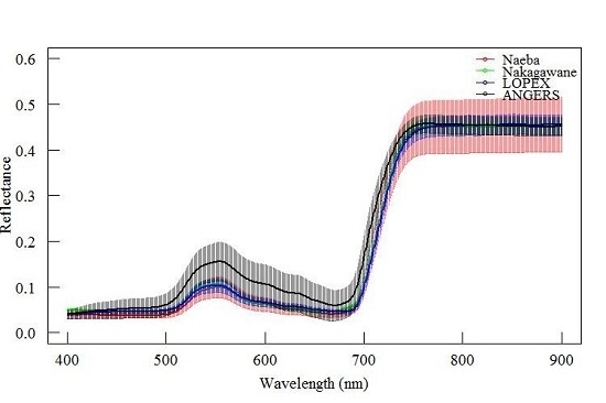
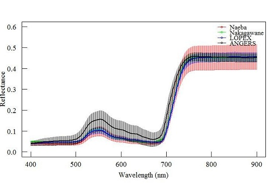
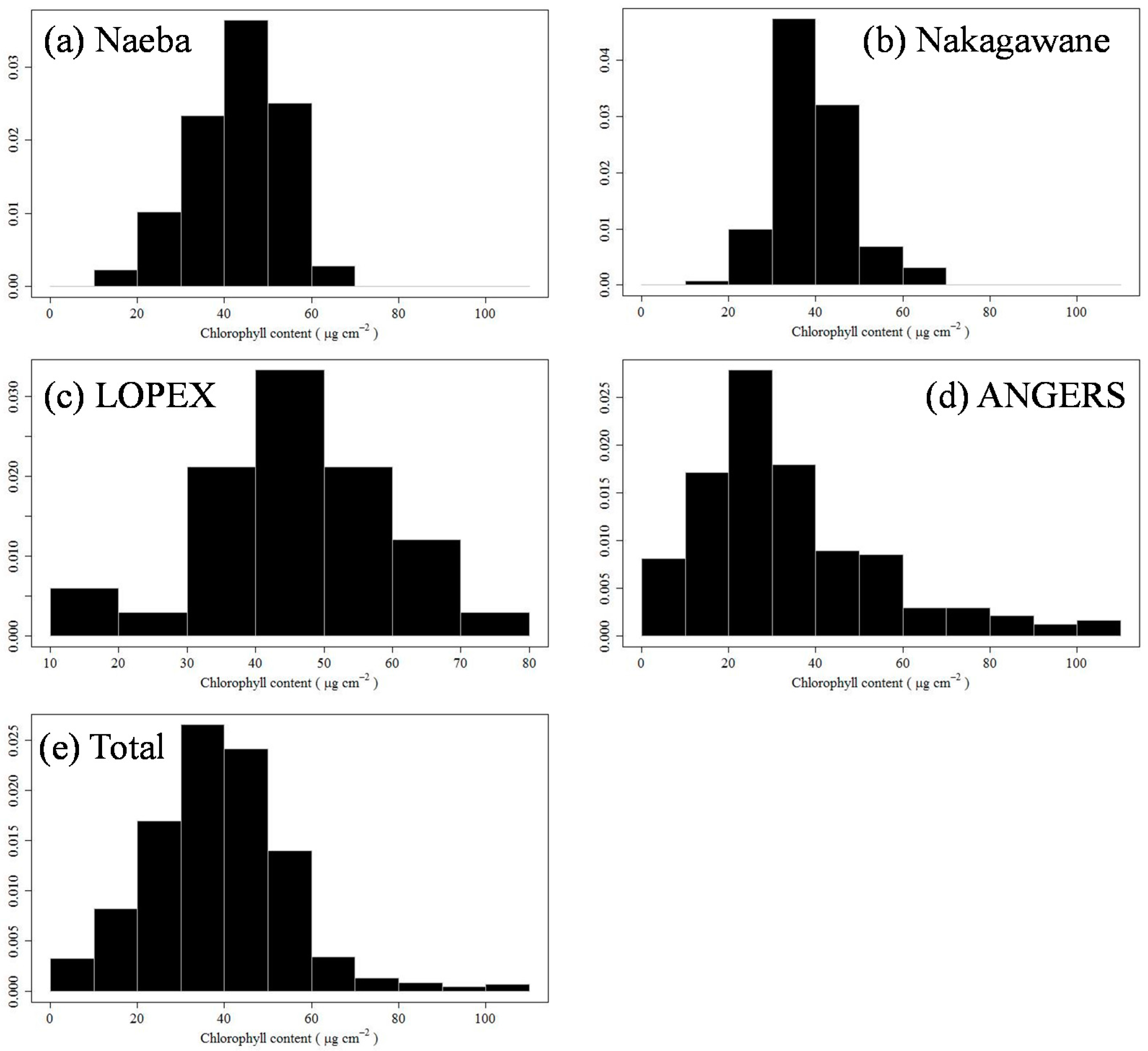
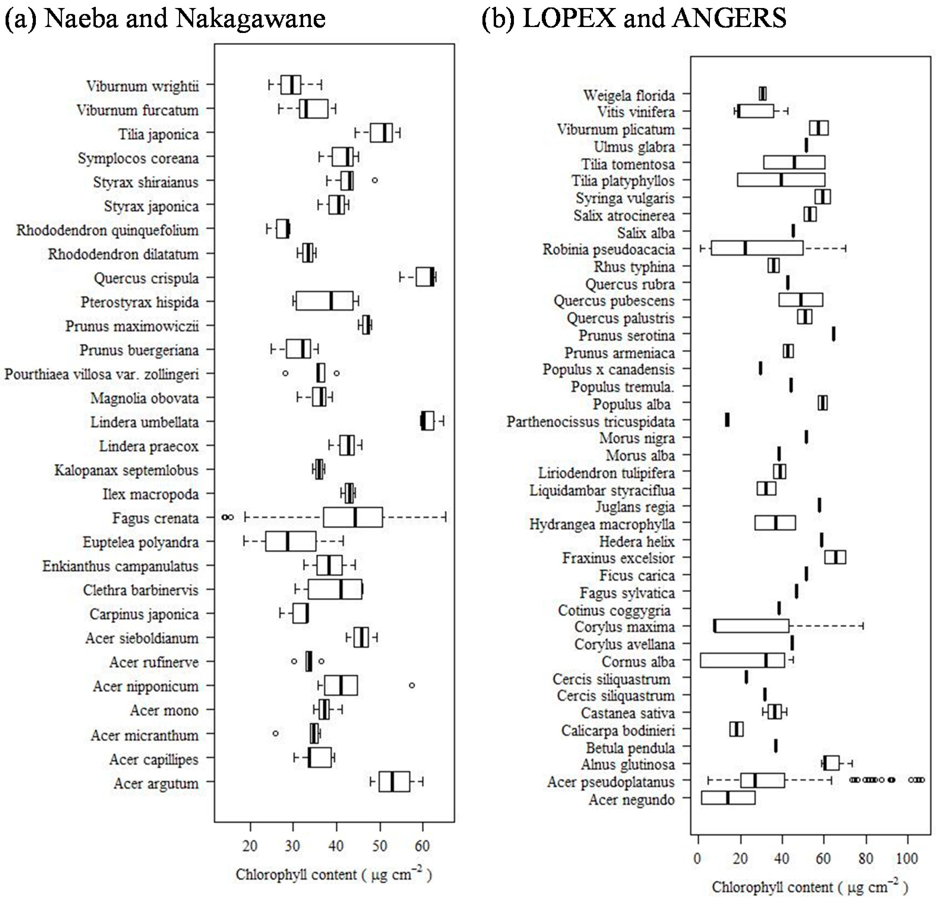
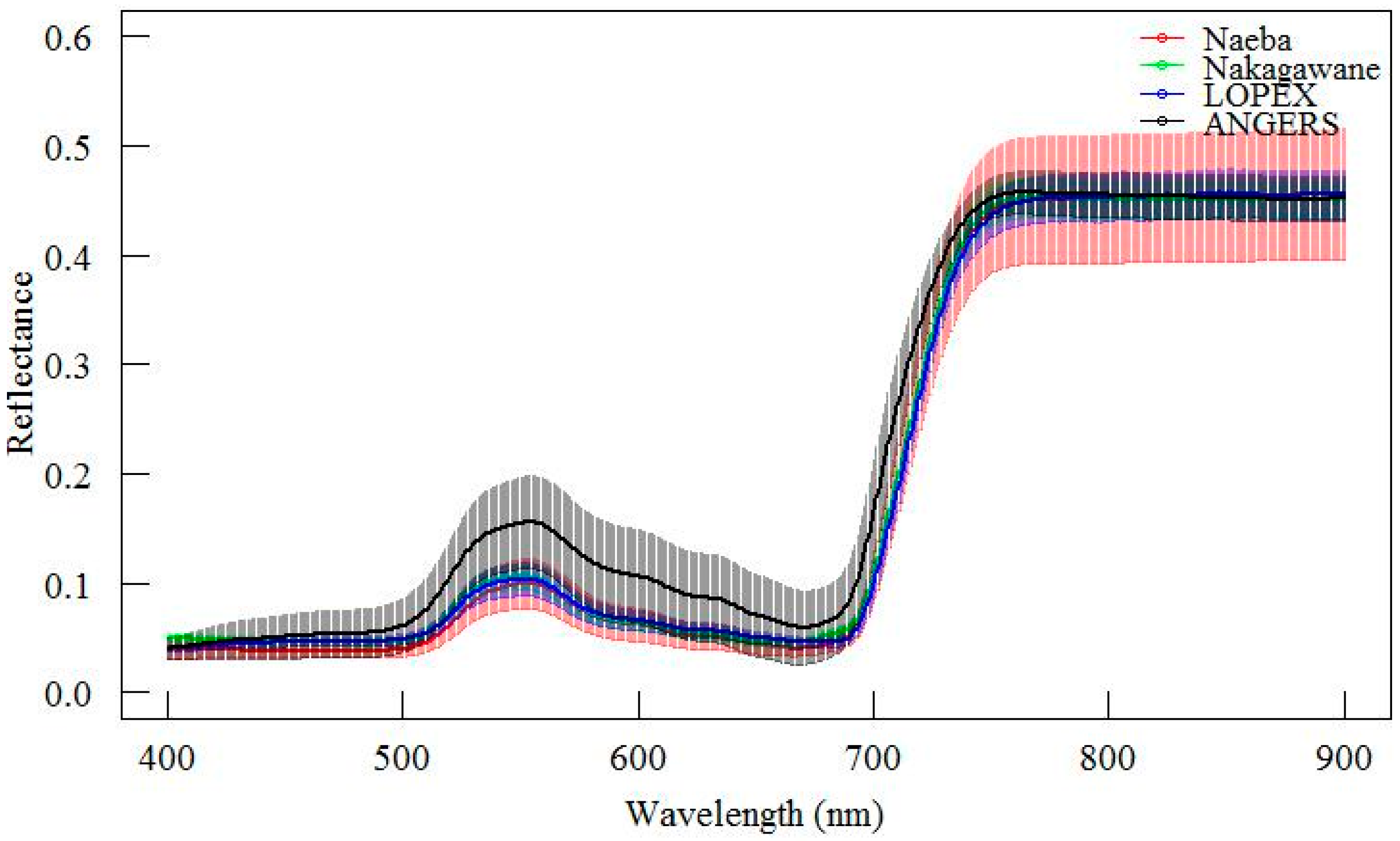
3.1. Chlorophyll Content of Each Dataset

Figure 2 shows the histogram distributions of chlorophyll concentrations of different broadleaf species for each dataset. For the measurements obtained in Naeba, the chlorophyll ranged from 13.94 to 65.18 μg/cm² with a median of 44.22 μg/cm². The mean value was estimated to be 42.88 μg/cm² and had a skewness of −0.538. Its standard deviation reached 10.50 μg/cm². As a comparison, the chlorophyll data obtained in Nakagawane, ranging from 18.58 to 64.76 μg/cm², had relatively lower values than in Naeba, with a lower median of 37.89 μg/cm², and a lower mean of 39.33 μg/cm² as well. Skewness was 0.661, and the standard deviation was 8.67 μg/cm², also lower than that of the data in Naeba.

For the two datasets obtained online, the chlorophyll concentrations in LOPEX covered a range from 18.49 to 70.39 μg/cm² with a median of 44.71 μg/cm², mean of 45.81 μg/cm², skewness of −0.189, and standard deviation of 12.20 μg/cm². For ANGERS, the chlorophyll concentrations covered a wider range, from 0.78 to 106.70 μg/cm² with median of 27.97 μg/cm², much smaller than that of LOPEX. Its mean value was also lower than that of LOPEX (33.15 μg/cm²), but a much larger standard deviation of 21.50 μg/cm² was found.

Figure 3 shows the descriptive statistics of chlorophyll content for each species. The lowest values were observed in Fagus crenata (13.94 μg/cm²) or Cornus alba (0.78 μg/cm²) for the two datasets and the online datasets, respectively. The largest values were also observed in Fagus crenata (65.18 μg/cm²) in the two field datasets, while Acer pseudoplatanus (106.71 μg/cm²) had the largest values for the online datasets. In the two field datasets, the variance of Fagus crenata was the largest among all the measurements, including other reported results in Japan (variance of 109.54). Corylus maxima had the largest variance among the online datasets, but it had only three measurements (variance of 1116.36). A significant difference was identified for the two field datasets and the two online datasets using the Tukey–Kramer test (p < 0.05), which yielded average values of 41.36 μg/cm² and 34.72 μg/cm², respectively.

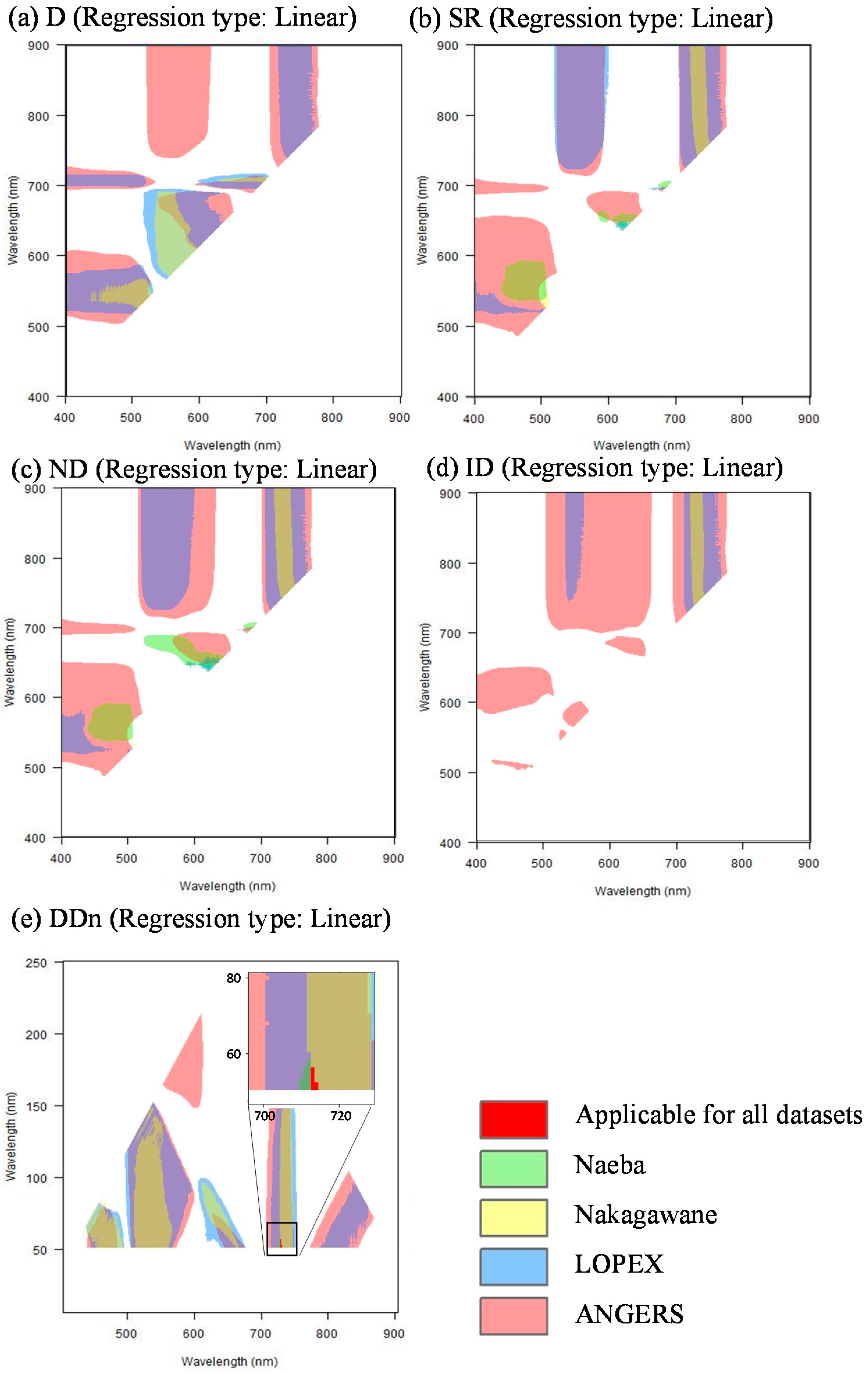
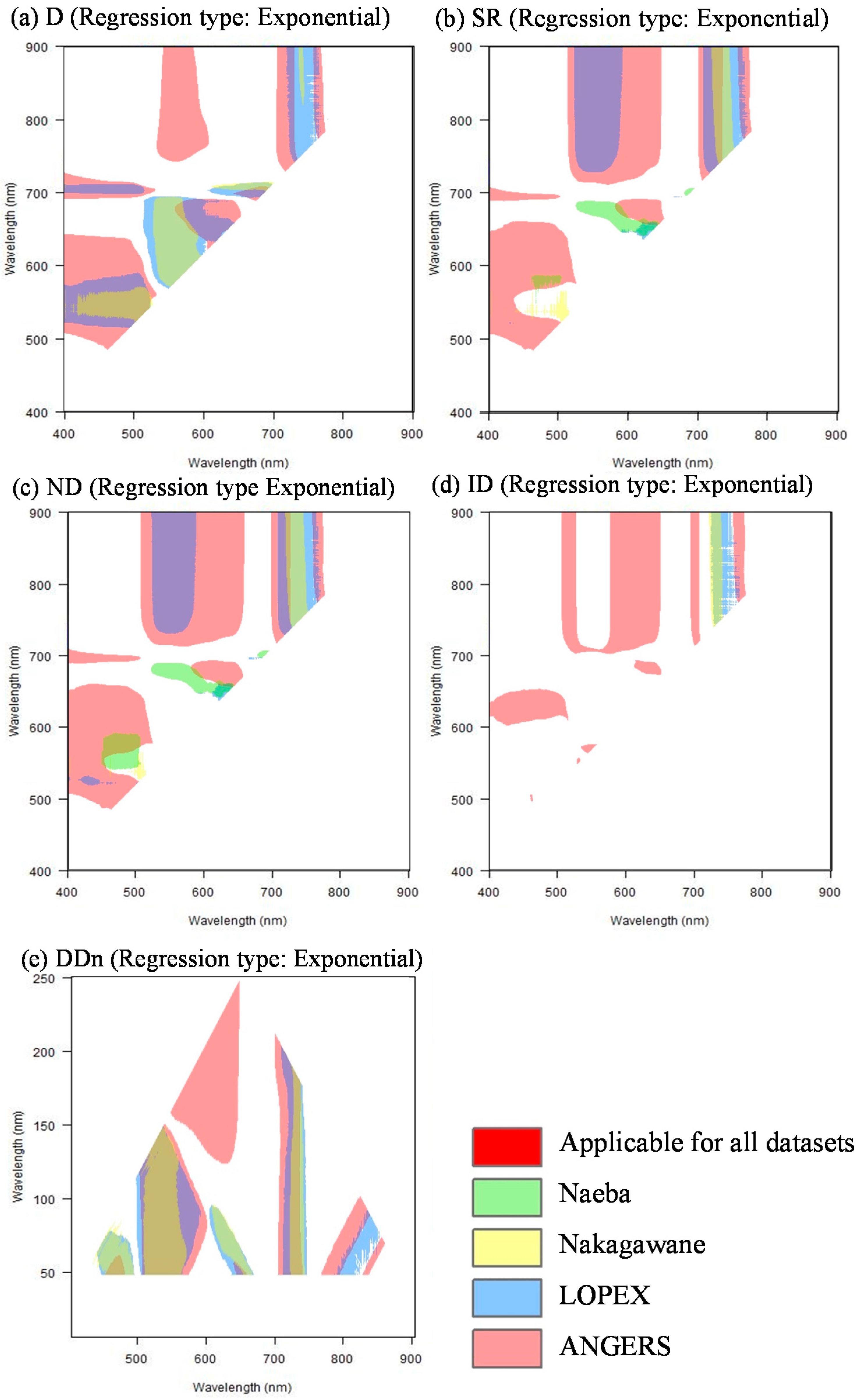
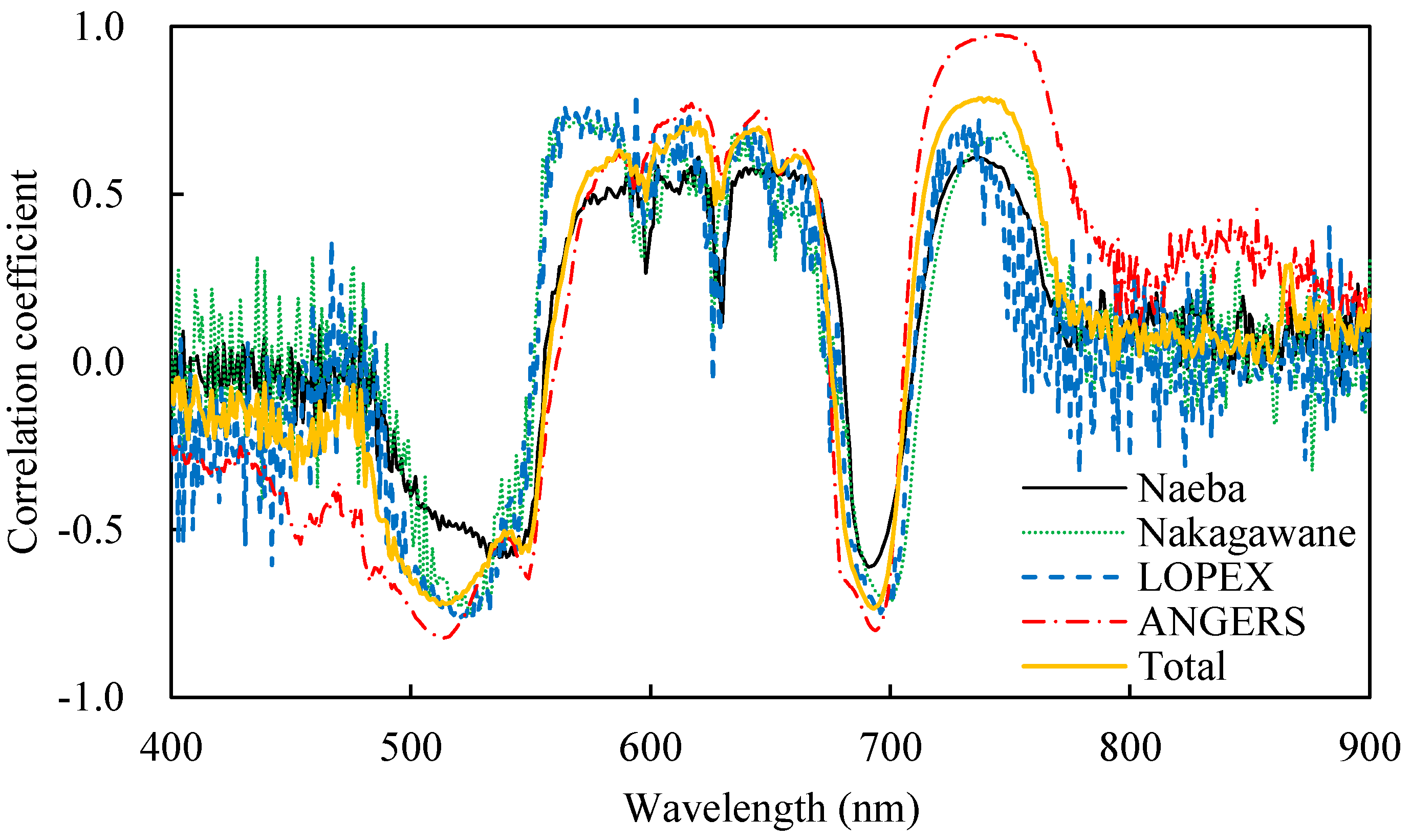
3.2. Identification of Optimal Indices for Estimating Chlorophyll Content Based on Original Spectra

Six common types of indices calculated from the original reflectance spectra were examined for their applications for each dataset. Linear and exponential regression types were examined for each index as well. Only those that were ranked as ‘A’ or ‘B’ for each dataset were illustrated (Figure 4 and Figure 5).

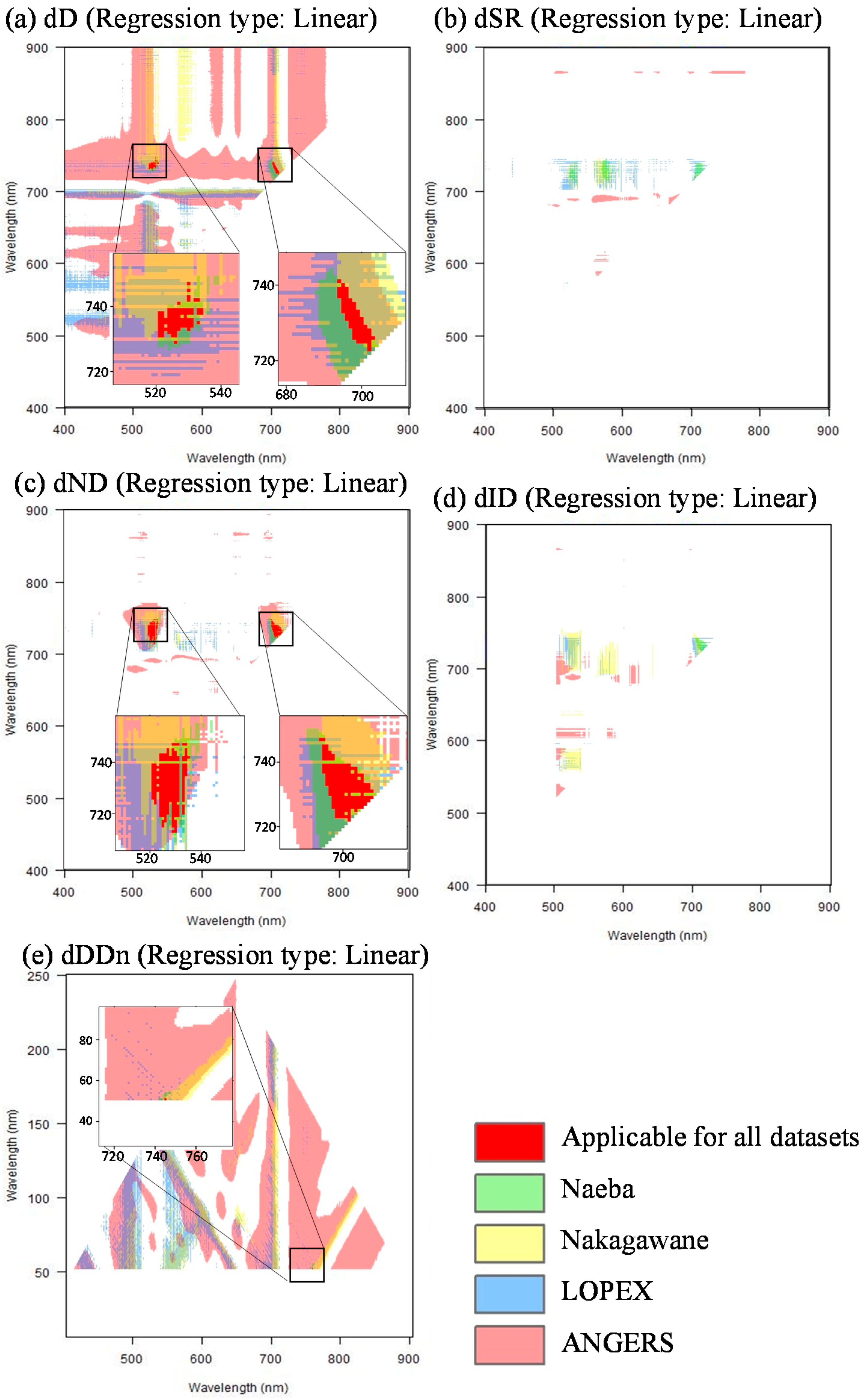
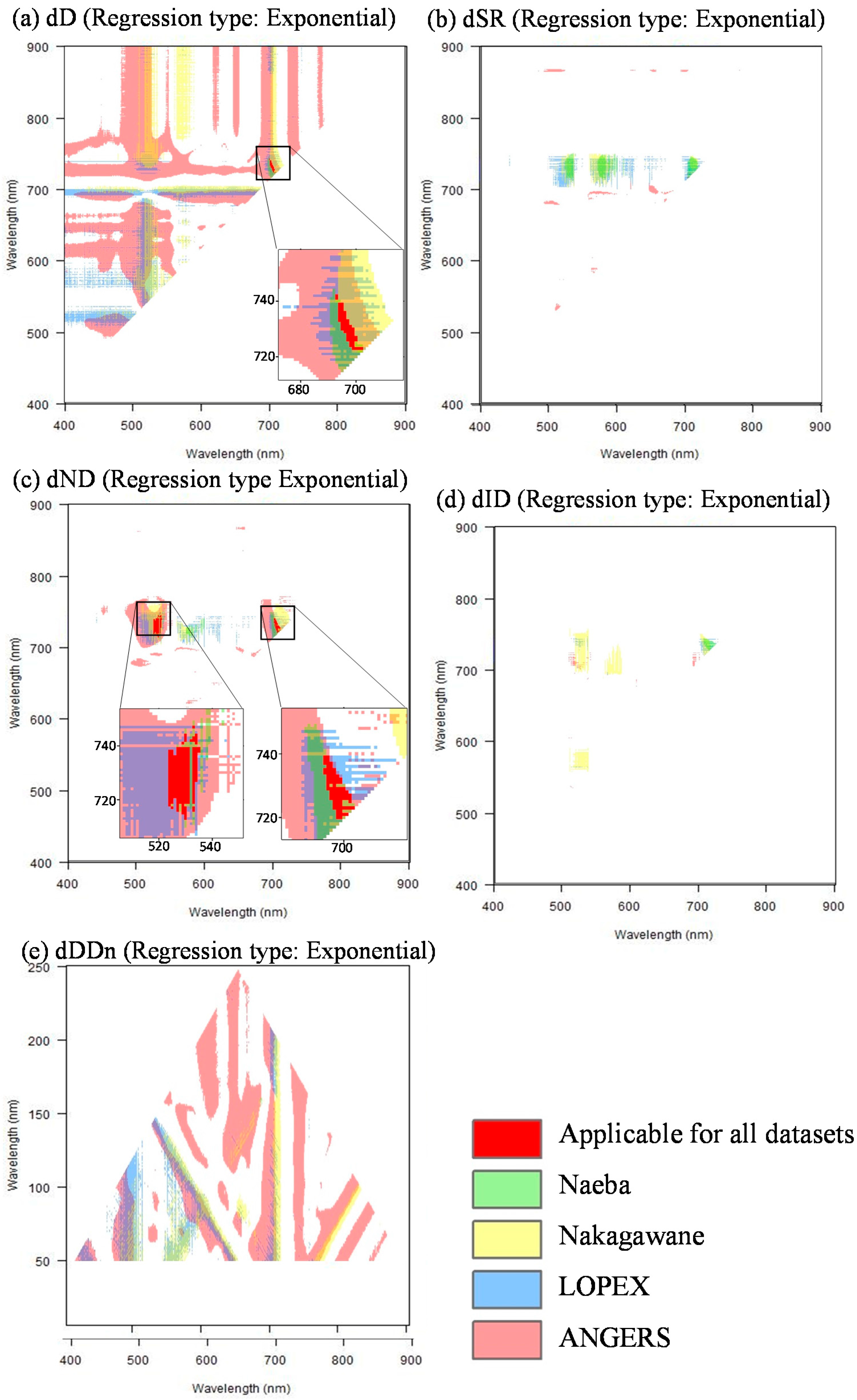
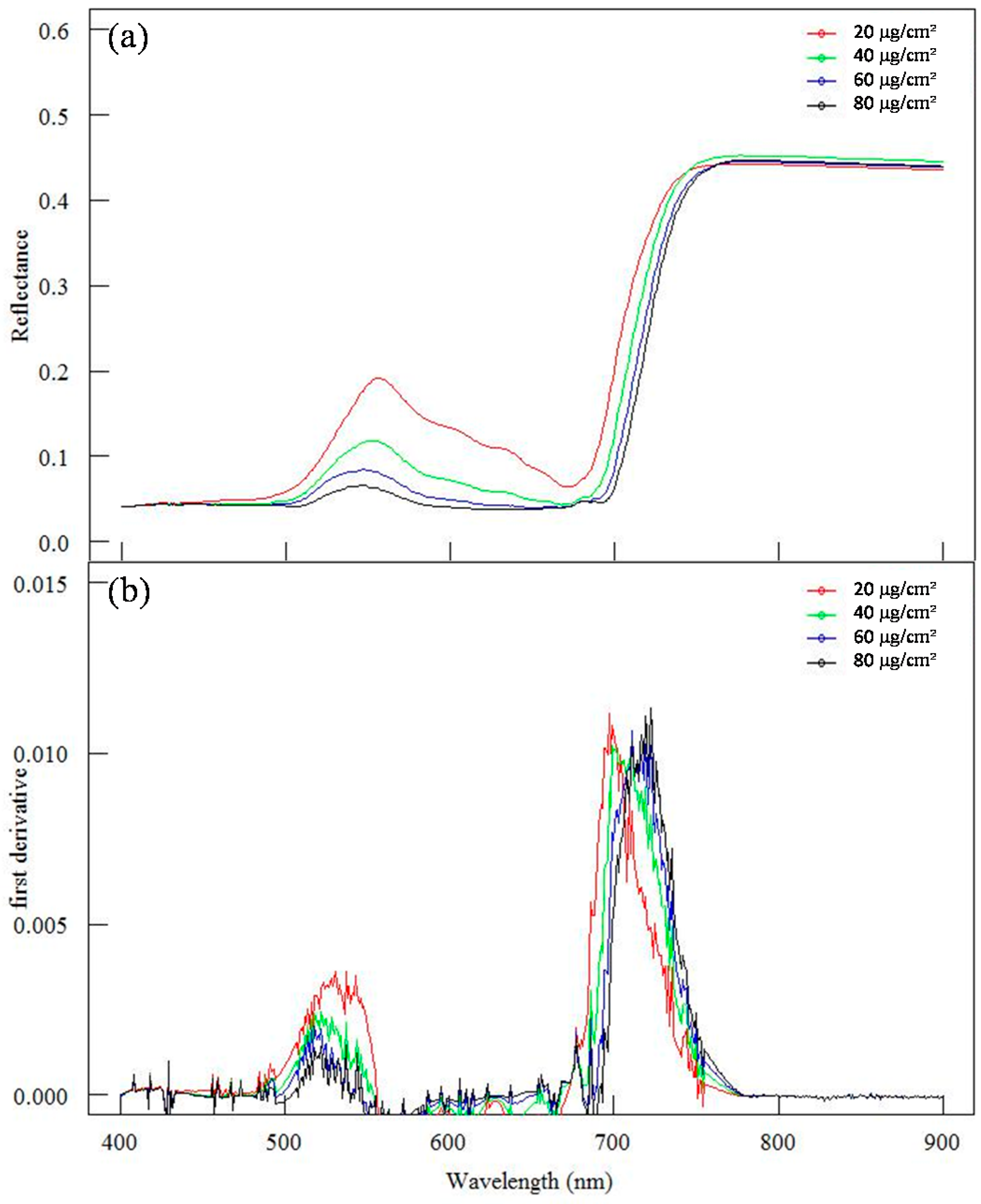
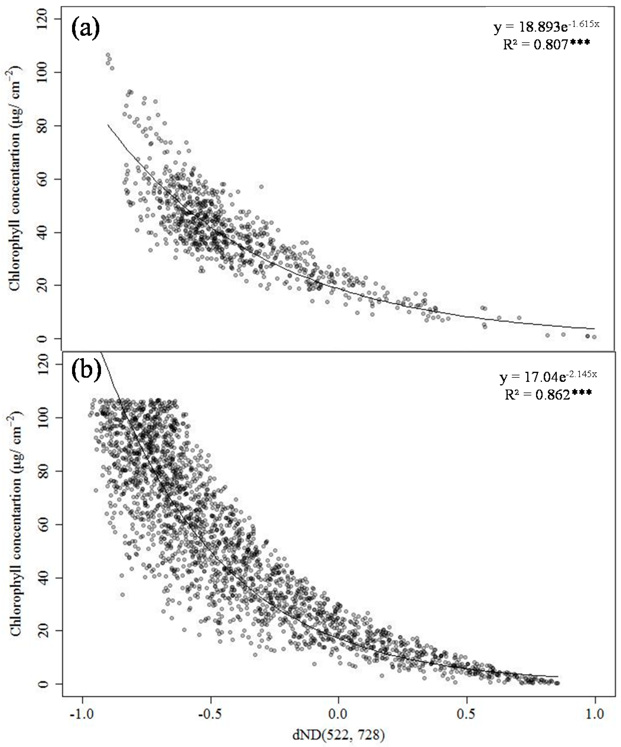
3.3. Identification of Optimal Indices Based on First-Order Derivative Spectra

Although there were many more combinations of each type of indices, most of them were not applicable for the other datasets beyond the datasets from which they had been developed, as revealed from Figure 4 and Figure 5. Instead, more indices that were applicable for all datasets were identified when using the first-order derivative-based indices (Figure 6 and Figure 7). Furthermore, the index types that performed best were different for those indices calculated from the original reflectance or first-order derivative spectra. In particular, the dD and dND index types were generally applicable for all datasets for those indices that used the combinations of reflectance near 740 nm and that near 520 or 695 nm, which were effective for qualifying chlorophyll concentrations (superior than B for both sites and leaf types). As a comparison, there were no applicable indices for the dSR or dID types; this was true for all datasets. Based on the RPD criterion, the indices including 174 combinations of dD types, 1 combination of dDDn type and 518 combinations of dND types were finally identified. Among them, those of the dND-type indices had RPD values higher than 1.9 when the four datasets were composited together.

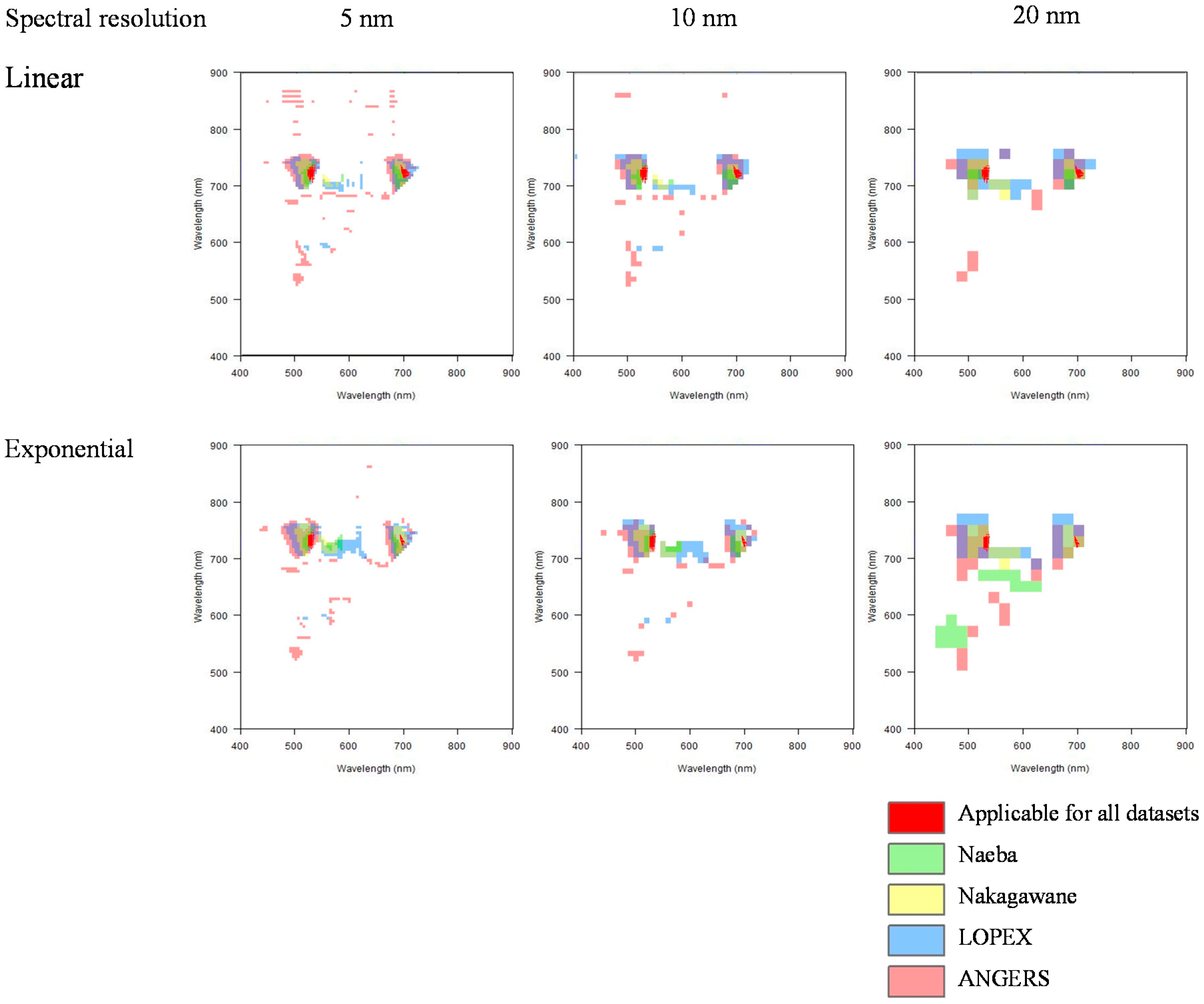
3.4. Evaluation of Indices with Down-Scaled Resolutions

The RPD changes with different spectral resolutions at 5, 10 or 20 nm. The trends for identified indices were analyzed in order to evaluate their consistence and the potential for the applications using reflectance information gathered from sensors on board satellites or aircraft. Generally, RPD values became lower with downscaled resolutions, and the relationships between chlorophyll concentrations and indices faded away gradually. Even so, the indices based on normalized differences (ND type) using first-order derivative spectra between the green peak (520–540 nm) and the end of the red edge (720–740 nm) proved to be the most robust indices, even when the resolution was downscaled to 20 nm. We were able to quantify chlorophyll concentrations for all datasets (Figure 8).

4. Discussion

4.1. Best indices for Each Dataset

Although respective best indices of ND (678, 698) (R² = 0.626, p < 0.001, WAIC = 2994.3), dID (533, 748) (R² = 0.640, p < 0.001, WAIC = 806.8), ND (741, 856) (R² = 0.776, p < 0.001, WAIC = 215.8) and ND (731,822) (R² = 0.960, p <0.001, WAIC = 1341.7) for Naeba, Nakagawane, LOPEX and ANGERS were identified by screening all combinations of different wavelengths using six index types, unfortunately, they were not applicable with other datasets beyond the one they were developed from (Figure 4, Figure 5, Figure 6 and Figure 7), which clearly indicates their specificity and lack of generality.

To discover the reasons for this, we first examined different spectra contained in the four datasets (a total of 816 measurements). Mean reflected spectra and their standard deviations for each dataset are presented in Figure 9. The results illustrate that although reflectance patterns are generally assembling, the reflectance values for the ANGERS dataset were higher than those of other datasets in visible and red-edge domains, resulting in the indices based on reflectance not being applicable for quantifying chlorophyll concentrations. Furthermore, different spectrophotometers used in various datasets might have caused serious bias on spectral data and thus affected the performance of identified indices from one dataset to other datasets (Perkin Elmer Lambda 19 double-beam spectrophotometer for LOPEX, ASD FieldSpec for other datasets) [14].

In contrast, the first-order derivative spectra, which may be calculated approximately by dividing the difference in reflectance between successive wavebands, can eliminate background noise and resolve overlapping spectral features [58]. This approach is effective in enhancing weak spectral features and extracting critical wavelengths by reducing the influence of trends or low-frequency noise [59]. It may therefore provide a solution towards identifying a general applicable index. Our results confirmed that, because the indices that performed best were applicable to all datasets, generally in different types based on the first-order derivative spectra. However, there were a few combinations of dID that were not suitable, especially LOPEX (Figure 6 and Figure 7).

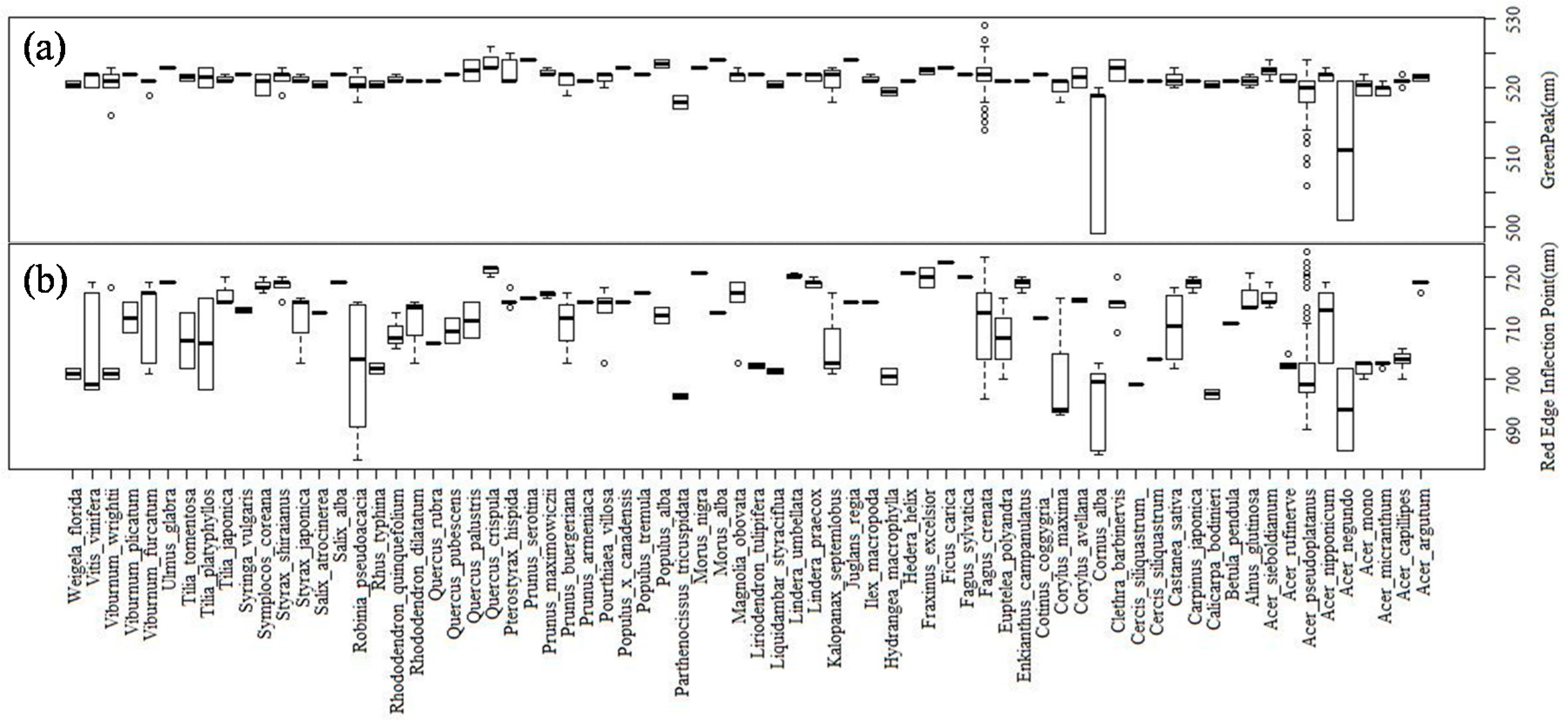
4.2. Most Popular Wavelengths Used in Indices That Performed Well

Figure 10 shows the correlations of each wavelength of first-order derivative spectra with chlorophyll content. Several peaks (positive correlations) and troughs (negative correlations) can be identified. Among them, one similar peak after 700 nm appeared at each dataset (peak wavelengths of 737, 748, 737, 744 and 741 nm for Naeba, Nakagawane, LOPEX, ANGERS and the total data when all four datasets were composed together, respectively). Two common troughs were found close to 520 nm (537, 525, 521, 513 and 512 nm for Naeba, Nakagawane, LOPEX, ANGERS and the total, respectively) and 695 nm (691, 698, 696, 694 and 693 nm for Naeba, Nakagawane, LOPEX, ANGERS and the total, respectively). Interestingly, all identified best indices generally used one wavelength that had a strong positive correlation (near the peak of 740 nm) and another wavelength that had a strong negative correlation (wavelengths near 520 or 695 nm), with the combinations of the wavelengths near 740 nm. Those near 520 nm had better performances, except for ANGERS.

The reflectance near 740 nm was located at the end of the red edge, and this position was also frequently used in feature indices for estimating chlorophyll content [60]. The reflectance at 550 nm was applied for estimating chlorophyll content in previous studies, where it is frequently noted as the green peak [31,39,61,62]. However, few studies have ever reported the effectiveness of reflectance near 520 nm. Actually, the wavelength of 520 nm corresponds to the maximum of the first-order derivative in the green domain for most deciduous species that were investigated in this study (Figure 11a). The difference in the green peak might be caused by different materials, since Carter and Knapp [31] report the shift among deciduous species. For the deciduous species, the reflectance near 695 nm was related to the red edge inflection point (REIP) (Figure 11b). Although the reflectance near 740 nm was related to the red edge position and adopted in previous studies [47], the red edge positions of deciduous species contained in this study were generally shorter than 740 nm. Its variation with different species was larger than that observed for the green peak positions of different species. That might be a reason that the green peak was superior to the red edge inflection point for quantifying chlorophyll concentrations.

4.3. Results from Measured Datasets vs. the Simulated Dataset

Figure 12 represents the reflectance and the first-order derivative spectra of the simulated dataset of 2500 samples. For simulated spectra, the green peak, which is a notable hill at 520–540 nm, became tiny with higher chlorophyll concentrations (Figure 12a). Furthermore, the red edge has shifted to longer wavelengths with higher chlorophyll concentrations (Figure 12b).

The tendencies observed in all datasets (Figure 10) were also noted and the peaks of positive correlations appeared at the wavelengths of 617 nm (R = 0.870) and 774 nm (R = 0.963), while those of negative correlations were observed at the wavelengths of 525nm (R = −0.778) and 689 nm (R = −0.863). The chlorophyll concentrations were again found to be significantly correlated with the first derivatives at the wavelengths of 522 nm (R = −0.707) and 728 nm (R = 0.811). Furthermore, the determination coefficient of 0.862 (p < 0.001, RMSE = 15.69 μg/cm², WAIC = 18507.6) between chlorophyll concentrations and the dND (522, 728), which had the best performance for all measured datasets, has confirmed the applicability of the index (Figure 13).

5. Conclusions

Diverse types of hyperspectral indices (reflectance at a given wavelength (R), wavelength difference (D), simple ratios (SR), normalized differences (ND) and double differences (DDn)) based on either original reflectance or first-order derivative spectra have been developed to quantify chlorophyll concentration using two datasets collected in situ from two typical cold-temperate mountainous sites in Japan and two online datasets (LOPEX and ANGERS). Furthermore, the best indices identified have further been evaluated using a simulated dataset generated from PROSPECT 5.

The robustness of identified indices among different datasets was evaluated using RPD values. These identified indices were generally from a combination of two wavelengths, in which one had a strong positive correlation and the other had a strong negative correlation with chlorophyll concentration. Overall, dND (522,728) proved to be the most effective index for quantifying chlorophyll concentrations (R² = 0.807, p < 0.001, RMSE = 8.67 μg/cm², WAIC = 5829.7) and was confirmed using the simulated dataset from PROSPECT 5 (R² = 0.862, p < 0.001, RMSE = 15.69 μg/cm², WAIC = 18507.6). Furthermore, the dND-type indices based on the first-order derivative spectra at the green peak (520–540 nm) and the end of the red edge (720–740 nm) were effective even for down-scaled resolutions (to 5, 10 and 20 nm), demonstrating great potential for the use of satellite data. The new understandings obtained in this study may thus help to improve the potential of hyperspectral remote sensing for quantifying chlorophyll concentrations.

References

1. Korus, A. Effect of preliminary and technological treatments on the content of chlorophylls and carotenoids in kale (Brassica oleracea L. Var. Acephala). J. Food Process. Preserv. 2013, 37, 335–344. [Google Scholar] [CrossRef]
2. Datt, B. Visible/near infrared reflectance and chlorophyll content in eucalyptus leaves. Int. J. Remote Sens. 1999, 20, 2741–2759. [Google Scholar] [CrossRef]
3. Atzberger, C.; Guerif, M.; Baret, F.; Werner, W. Comparative analysis of three chemometric techniques for the spectroradiometric assessment of canopy chlorophyll content in winter wheat. Comput. Electron. Agric. 2010, 73, 165–173. [Google Scholar] [CrossRef]
4. Mattos, E.R.; Singh, M.; Cabrera, M.L.; Das, K.C. Enhancement of biomass production in scenedesmus bijuga high-density culture using weakly absorbed green light. Biomass Bioenergy 2015, 81, 473–478. [Google Scholar] [CrossRef]
5. Zarco-Tejada, P.J.; Miller, J.R.; Noland, T.L.; Mohammed, G.H.; Sampson, P.H. Scaling-up and model inversion methods with narrowband optical indices for chlorophyll content estimation in closed forest canopies with hyperspectral data. IEEE Trans. Geosci. Remote Sens. 2001, 39, 1491–1507. [Google Scholar] [CrossRef]
6. Collins, W. Remote sensing of crop type and maturity. Photogramm. Eng. Remote Sens. 1978, 44, 43–55. [Google Scholar]
7. Filella, I.; Amaro, T.; Araus, J.L.; Penuelas, J. Relationship between photosynthetic radiation-use efficiency of barley canopies and the photochemical reflectance index (PRI). Physiol. Plant. 1996, 96, 211–216. [Google Scholar] [CrossRef]
8. Horler, D.N.H.; Dockray, M.; Barber, J. The red edge of plant leaf reflectance. Int. J. Remote Sens. 1983, 4, 273–288. [Google Scholar] [CrossRef]
9. Miller, J.R.; Hare, E.W.; Wu, J. Quantitative characterisation of the red edge reflectance 1. An inverted-gaussian model. Int. J. Remote Sens. 1990, 11, 1755–1773. [Google Scholar] [CrossRef]
10. Elvidge, C.D.; Chen, Z.K. Comparison of broad-band and narrow-band red and near-infrared vegetation indices. Remote Sens. Environ. 1995, 54, 38–48. [Google Scholar] [CrossRef]
11. Filella, I.; Serrano, L.; Serra, J.; Penuelas, J. Evaluating wheat nitrogen status with canopy reflectance indices and discriminant analysis. Crop Sci. 1995, 35, 1400–1405. [Google Scholar] [CrossRef]
12. Sonobe, R.; Wang, Q. Hyperspectral indices for quantifying leaf chlorophyll concentrations performed differently with different leaf types in deciduous forests. Ecol. Inform. 2017, 37, 1–9. [Google Scholar] [CrossRef]
13. Hosgood, B.; Jacquemoud, S.; Andreoli, G.; Verdebout, J.; Pedrini, G.; Schmuck, G. Leaf Optical Properties Experiment 93 (Lopex93); European Commission—Joint Research Centre: Ispra, Italy, 1994; p. 20. [Google Scholar]
14. Féret, J.-B.; Francois, C.; Asner, G.P.; Gitelson, A.A.; Martin, R.E.; Bidel, L.P.R.; Ustin, S.L.; le Maire, G.; Jacquemoud, S. PROSPECT-4 and 5: Advances in the leaf optical properties model separating photosynthetic pigments. Remote Sens. Environ. 2008, 112, 3030–3043. [Google Scholar] [CrossRef]
15. Marshall, M.; Thenkabail, P. Advantage of hyperspectral EO-1 Hyperion over multispectral IKONOS, GeoEye-1, WorldView-2, Landsat ETM plus, and MODIS vegetation indices in crop biomass estimation. ISPRS J. Photogramm. Remote Sens. 2015, 108, 205–218. [Google Scholar] [CrossRef]
16. Yamamoto, H.; Kouyama, T.; Obata, K.; Tsuchida, S. Assessment of hisui radiometric performance using vicarious calibration and cross-calibration. In Proceedings of the 2015 IEEE International Geoscience and Remote Sensing Symposium, Milan, Italy, 26–31 July 2015; pp. 2805–2808.
17. Yamamoto, H.; Nakamura, R.; Tsuchida, S. Radiometric Calibration Plan for the Hyperspectral Imager Suite (HISUI) Instruments. In Proceedings of the Conference on Multispectral, Hyperspectral, and Ultraspectral Remote Sensing Technology, Techniques and Applications IV, Kyoto, Japan, 30–31 October 2012.
18. Williams, P. Variables affecting near-infraredreflectance spectroscopic analysis. In Near-Infrared Technology in the agricultural and Food Industries; Williams, P., Norris, K., Eds.; American Association of Cereal Chemists Inc.: St. Paul, MN, USA, 1987; pp. 143–167. [Google Scholar]
19. Minasny, B.; McBratney, A. Why you don’t need to use RPD. Pedometron 2013, 33, 14–15. [Google Scholar]
20. Watanabe, S. Asymptotic equivalence of bayes cross validation and widely applicable information criterion in singular learning theory. J. Mach. Learn. Res. 2010, 11, 3571–3594. [Google Scholar]
21. Japan Meteorological Agency. Available online: http://www.data.jma.go.jp/ (accessed on 23 January 2017).
22. Gamon, J.A.; Rahman, A.F.; Dungan, J.L.; Schildhauer, M.; Huemmrich, K.F. Spectral Network (SpecNet)-What is it and why do we need it? Remote Sens. Environ. 2006, 103, 227–235. [Google Scholar] [CrossRef]
23. Wang, Q.; Iio, A.; Tenhunen, J.; Kakubari, Y. Annual and seasonal variations in photosynthetic capacity of Fagus crenata along an elevation gradient in the Naeba Mountains, Japan. Tree Physiol. 2008, 28, 277–285. [Google Scholar] [CrossRef]
24. Iwasaki, T.; Aoki, K.; Seo, A.; Murakami, N. Comparative phylogeography of four component species of deciduous broad-leaved forests in japan based on chloroplast dna variation. J. Plant Res. 2012, 125, 207–221. [Google Scholar] [CrossRef] [PubMed]
25. Takahara, H.; Takeoka, M. Vegetation history since the last glacial period in the Mikata lowland, the Sea of Japan area, western Japan. Ecol. Res. 1992, 7, 371–386. [Google Scholar] [CrossRef]
26. Foley, S.; Rivard, B.; Sanchez-Azofeifa, G.A.; Calvo, J. Foliar spectral properties following leaf clipping and implications for handling techniques. Remote Sens. Environ. 2006, 103, 265–275. [Google Scholar] [CrossRef]
27. Richardson, A.D.; Berlyn, G.P. Changes in foliar spectral reflectance and chlorophyll fluorescence of four temperate species following branch cutting. Tree Physiol. 2002, 22, 499–506. [Google Scholar] [CrossRef] [PubMed]
28. Arnon, D.I. Copper enzymes in isolated chloroplasts. Polyphenoloxidase in beta vulgaris. Plant Physiol. 1949, 24, 1–15. [Google Scholar] [CrossRef] [PubMed]
29. Pavan, G.; Jacquemoud, S.; Bidel, L.; Francois, C.; de Rosny, G.; Rambaut, J.P.; Frangi, J.P. Ramis: A new portable field radiometer to estimate leaf biochemical content. In Proceedings of the 7th International Conference on Precision Agriculture and Other Precision Resources Management, Minneapolis, MN, USA, 25–28 July 2004; p. 14.
30. Boochs, F.; Kupfer, G.; Dockter, K.; Kuhbauch, W. Shape of the red edge as vitality indicator for plants. Int. J. Remote Sens. 1990, 11, 1741–1753. [Google Scholar] [CrossRef]
31. Carter, G.A.; Knapp, A.K. Leaf optical properties in higher plants: Linking spectral characteristics to stress and chlorophyll concentration. Am. J. Bot. 2001, 88, 677–684. [Google Scholar] [CrossRef] [PubMed]
32. Gamon, J.A.; Surfus, J.S. Assessing leaf pigment content and activity with a reflectometer. New Phytol. 1999, 143, 105–117. [Google Scholar] [CrossRef]
33. Tanaka, S.; Kawamura, K.; Maki, M.; Muramoto, Y.; Yoshida, K.; Akiyama, T. Spectral Index for Quantifying Leaf Area Index of Winter Wheat by Field Hyperspectral Measurements: A Case Study in Gifu Prefecture, Central Japan. Remote Sens. 2015, 7, 5329–5346. [Google Scholar] [CrossRef]
34. Sonobe, R.; Wang, Q. Assessing the xanthophyll cycle in natural beech leaves with hyperspectral reflectance. Funct. Plant Biol. 2016, 43, 438–447. [Google Scholar] [CrossRef]
35. Blackburn, G.A. Spectral indices for estimating photosynthetic pigment concentrations: A test using senescent tree leaves. Int. J. Remote Sens. 1998, 19, 657–675. [Google Scholar] [CrossRef]
36. Blackburn, G.A. Quantifying chlorophylls and caroteniods at leaf and canopy scales: An evaluation of some hyperspectral approaches. Remote Sens. Environ. 1998, 66, 273–285. [Google Scholar] [CrossRef]
37. Carter, G.A. Ratios of leaf reflectances in narrow wavebands as indicators of plant stress. Int. J. Remote Sens. 1994, 15, 697–703. [Google Scholar] [CrossRef]
38. Chappelle, E.W.; Kim, M.S.; McMurtrey, J.E. Ratio analysis of reflectance spectra (RARS): An algorithm for the remote estimation of the concentrations of chlorophyll A, chlorophyll B, and carotenoids in soybean leaves. Remote Sens. Environ. 1992, 39, 239–247. [Google Scholar] [CrossRef]
39. Datt, B. Remote sensing of chlorophyll a, chlorophyll b, chlorophyll a+b, and total carotenoid content in eucalyptus leaves. Remote Sens. Environ. 1998, 66, 111–121. [Google Scholar] [CrossRef]
40. Datt, B. A new reflectance index for remote sensing of chlorophyll content in higher plants: Tests using eucalyptus leaves. J. Plant Physiol. 1999, 154, 30–36. [Google Scholar] [CrossRef]
41. Gitelson, A.A.; Merzlyak, M.N. Signature analysis of leaf reflectance spectra: Algorithm development for remote sensing of chlorophyll. J. Plant Physiol. 1996, 148, 494–500. [Google Scholar] [CrossRef]
42. Jordan, C.F. Derivation of leaf-area index from quality of light on the forest floor. Ecology 1969, 50, 663–666. [Google Scholar] [CrossRef]
43. Lichtenthaler, H.K.; Lang, M.; Sowinska, M.; Heisel, F.; Miehe, J.A. Detection of vegetation stress via a new high resolution fluorescence imaging system. J. Plant Physiol. 1996, 148, 599–612. [Google Scholar] [CrossRef]
44. McMurtrey, J.E.; Chappelle, E.W.; Kim, M.S.; Meisinger, J.J.; Corp, L.A. Distinguishing nitrogen fertilization levels in field corn (Zea mays L.) with actively induced fluorescence and passive reflectance measurements. Remote Sens. Environ. 1994, 47, 36–44. [Google Scholar] [CrossRef]
45. Penuelas, J.; Filella, I.; Biel, C.; Serrano, L.; Save, R. The reflectance at the 950–970 nm region as an indicator of plant water status. Int. J. Remote Sens. 1993, 14, 1887–1905. [Google Scholar] [CrossRef]
46. Smith, R.C.G.; Adams, J.; Stephens, D.J.; Hick, P.T. Forecasting wheat yield in a mediterranean-type environment from the noaa satellite. Aust. J. Agric. Res. 1995, 46, 113–125. [Google Scholar] [CrossRef]
47. Vogelmann, J.E.; Rock, B.N.; Moss, D.M. Red edge spectral measurements from sugar maple leaves. Int. J. Remote Sens. 1993, 14, 1563–1575. [Google Scholar] [CrossRef]
48. Zarco-Tejada, P.J.; Miller, J.R.; Haboudane, D.; Tremblay, N.; Apostol, S. Detection of chlorophyll fluorescence in vegetation from airborne hyperspectral casi imagery in the red edge spectral region. In Proceedings of the 2003 IEEE International Geoscience and Remote Sensing Symposium, Toulouse, France, 21–25 July 2003; pp. 598–600.
49. Zarco-Tejada, P.J.; Pushnik, J.C.; Dobrowski, S.; Ustin, S.L. Steady-state chlorophyll a fluorescence detection from canopy derivative reflectance and double-peak red-edge effects. Remote Sens. Environ. 2003, 84, 283–294. [Google Scholar] [CrossRef]
50. Gandia, S.; Fernández, G.; Moreno, J. Retrieval of vegetation biophysical variables from chris/proba data in the sparc campaign. In Proceedings of the 2nd CHRIS/Proba Workshop, Frascati, Italy, 28–30 April 2004; ESA/ESRIN: Frascati, Italy; pp. 40–48.
51. Gitelson, A.; Merzlyak, M.N. Spectral reflectance changes associated with autumn senescence of Aesculus hippocastanum L. and Acer platanoides L. Leaves. Spectral features and relation to chlorophyll estimation. J. Plant Physiol. 1994, 143, 286–292. [Google Scholar] [CrossRef]
52. le Maire, G.; Francois, C.; Soudani, K.; Berveiller, D.; Pontailler, J.Y.; Breda, N.; Genet, H.; Davi, H.; Dufrene, E. Calibration and validation of hyperspectral indices for the estimation of broadleaved forest leaf chlorophyll content, leaf mass per area, leaf area index and leaf canopy biomass. Remote Sens. Environ. 2008, 112, 3846–3864. [Google Scholar] [CrossRef]
53. Wang, Q.; Li, P. Identification of robust hyperspectral indices on forest leaf water content using prospect simulated dataset and field reflectance measurements. Hydrol. Process. 2012, 26, 1230–1241. [Google Scholar] [CrossRef]
54. Gitelson, A.A.; Merzlyak, M.N.; Chivkunova, O.B. Optical properties and nondestructive estimation of anthocyanin content in plant leaves. Photochem. Photobiol. 2001, 74, 38–45. [Google Scholar] [CrossRef]
55. Gitelson, A.A.; Zur, Y.; Chivkunova, O.B.; Merzlyak, M.N. Assessing carotenoid content in plant leaves with reflectance spectroscopy. Photochem. Photobiol. 2002, 75, 272–281. [Google Scholar] [CrossRef]
56. Chang, C.W.; Laird, D.A.; Mausbach, M.J.; Hurburgh, C.R. Near-infrared reflectance spectroscopy-principal components regression analyses of soil properties. Soil Sci. Soc. Am. J. 2001, 65, 480–490. [Google Scholar] [CrossRef]
57. Scott, D. Multivariate Density Estimation: Theory, Practice, and Visualization; Wiley: New York, NY, USA, 1992. [Google Scholar]
58. Lawley, V.; Lewis, M.; Clarke, K.; Ostendorf, B. Site-based and remote sensing methods for monitoring indicators of vegetation condition: An australian review. Ecol. Indic. 2016, 60, 1273–1283. [Google Scholar] [CrossRef]
59. Inoue, Y.; Sakaiya, E.; Zhu, Y.; Takahashi, W. Diagnostic mapping of canopy nitrogen content in rice based on hyperspectral measurements. Remote Sens. Environ. 2012, 126, 210–221. [Google Scholar] [CrossRef]
60. Sanches, I.D.A.; Souza Filho, C.R.; Kokaly, R.F. Spectroscopic remote sensing of plant stress at leaf and canopy levels using the chlorophyll 680 nm absorption feature with continuum removal. ISPRS J. Photogramm. Remote Sens. 2014, 97, 111–122. [Google Scholar] [CrossRef]
61. Broge, N.H.; Leblanc, E. Comparing prediction power and stability of broadband and hyperspectral vegetation indices for estimation of green leaf area index and canopy chlorophyll density. Remote Sens. Environ. 2001, 76, 156–172. [Google Scholar] [CrossRef]
62. Gitelson, A.A.; Kaufman, Y.J.; Merzlyak, M.N. Use of a green channel in remote sensing of global vegetation from eos-modis. Remote Sens. Environ. 1996, 58, 289–298. [Google Scholar] [CrossRef]
Figure 1. Locations of Mount Naeba and Nakagawane in Japan.
Remotesensing 09 00191 g001
Figure 2. Histograms of chlorophyll content for (a) Naeba; (b) Nakagawane; (c) the Joint Research Centre Leaf Optical Properties Experiment (LOPEX); (d) the dataset measured in 2003 at INRA in Angers, France (ANGERS) and (e) Total. The histograms were expressed using Scott’s method [57].
Remotesensing 09 00191 g002
Figure 3. Changes in chlorophyll content for each species; (a) our datasets (Naeba and Nakagawane) and (b) published datasets (LOPEX and ANGERS). Boxes encompass the 25% and 75% quartiles of the entire dataset. The central solid line represents the median. Bars extend to the 95% confidence limits. Dots represent outliers.
Remotesensing 09 00191 g003
Figure 4. Categories based on ratio of performance to deviation (RPD) with different type indices using original reflectance (linear regression). D: wavelength difference; SR: simple ratios; ND: normalized difference; DDn: double differences; ID: inverse reflectance differences.
Remotesensing 09 00191 g004
Figure 5. Categories based on RPD with different type indices using original reflectance (exponential regression).
Remotesensing 09 00191 g005
Figure 6. Categories based on RPD with different type indices using first-order derivative spectra (linear regression).
Remotesensing 09 00191 g006
Figure 7. Categories based on RPD with different types of indices using first-order derivative spectra (exponential regression).
Remotesensing 09 00191 g007
Figure 8. RPD changes with resolution down. Colored areas represent useful combinations for quantifying chlorophyll concentrations for each dataset (categorized ‘A’ or ‘B’ based on RPD values).
Remotesensing 09 00191 g008
Figure 9. Mean reflectance spectra and standard deviations. Solid lines represent mean reflectance and thinner zones represent standard deviations.
Remotesensing 09 00191 g009
Figure 10. Correlations between first-order derivative spectra and chlorophyll content.
Remotesensing 09 00191 g010
Figure 11. (a) Green peak and (b) red edge positions for deciduous species considered in this study.
Remotesensing 09 00191 g011
Figure 12. (a) Mean reflectance spectra and (b) first-order derivative spectra simulated by PROpriétés SPECTrales Version 5 (PROSPECT 5).
Remotesensing 09 00191 g012
Figure 13. The relationship between dND (522, 728) and chlorophyll content (a) for measured datasets and (b) a simulated dataset from PROpriétés SPECTrales (PROSPECT) Version 5 (*** indicates p < 0.001).
Remotesensing 09 00191 g013