Article

An Improved Automatic Algorithm for Global Eddy Tracking Using Satellite Altimeter Data

1
College of Information Science and Engineering, Ocean University of China, Qingdao 266100, China
2
Laboratory for Regional Oceanography and Numerical Modeling, Qingdao National Laboratory for Marine Science and Technology, Qingdao 266100, China
*
Author to whom correspondence should be addressed.
Remote Sens. 2017, 9(3), 206; https://doi.org/10.3390/rs9030206
Submission received: 3 November 2016 / Revised: 21 February 2017 / Accepted: 22 February 2017 / Published: 25 February 2017

Abstract

:
In this paper, we propose a new hybrid mesoscale eddy tracking method to enhance the eddy tracking accuracy from global satellite altimeter data. This method integrates both physical and geometric eddy properties (including the distance between eddies, the area and amplitude of eddy, and the shape of the eddy edge) via the output of detection and the calculation of Hausdorff distance, which could describe the similarity between eddy boundaries. We applied the proposed hybrid method to several previously reported eddies and compared the results with those from two traditional tracking methods. A quantitative comparison indicates that the hybrid algorithm can better reveal eddy signals in terms of their spatial scale, amplitude, lifespan, and splitting. The hybrid method was used for global mesoscale eddies tracking from 1993 to 2015. Global distributions of net eddy numbers revealed that the sources of eddies are located along the eastern boundaries of the world oceans, while the sinks of eddies are located along the western boundaries. The lifespan distribution of eddies exhibited steep growth from high and low latitudes to middle latitudes. A clear divergent pathway demonstrates that cyclonic/anticyclonic eddies tend to travel poleward/equatorward in the world oceans.

1. Introduction

Mesoscale eddies are large bodies of swirling water with scales ranging from ten to hundreds of kilometres and with lifespans ranging from days to years [1,2,3]. They are ubiquitous in the world oceans and play a major role in the kinetic energy balance of the ocean, primary production, heat transfer and air-sea interactions [4,5,6,7,8,9]. Accurate detecting and tracking eddies is a key preliminary step in gaining a better understanding of their physical properties, transport, circulation, evolution, decay and their impact on other ocean processes.
Satellite altimeter data from 23 years allows us to carry out mesoscale eddy investigations in large-scale and long time series. In the literature, methods for detecting and tracking mesoscale eddies have been developed. The eddy detection methods are mainly categorized into three types: (1) methods based on eddy inherit parameters, such as the Okubo-Weiss (OW) method; (2) eddy geometry-based methods, including the eddy-induced sea level anomaly (SLA)-based method; and (3) hybrid methods, which use both physical parameters and flow pattern associated with eddies. The eddy tracking methods have attracted a great deal of attention to understand different scientific problems [10,11,12,13,14,15,16]. The first school of tracking methods is referred to as the similarity method. Penven et al. [17] first used the Euclidean distance of non-dimensional eddy properties to describe and match eddy similarities in two sets of successive altimeter data. This method and its improved version have been widely used for mesoscale eddy tracking globally [2,18,19,20,21]. The second type of popular eddy tracking methods adopted by [2,22] consist of finding the closest eddy centre and using loose limitations to constrain the search results in two contiguous time steps [16,23]. This type of method (hereafter termed the CH11 method) differs from a similarity method because it uses only threshold limitations to end the tracking calculation. For example, Doglioli et al. [24] and Xiu et al. [25] employed the CH11 method to extract eddy signals to understand characteristics of regional eddies.
Many studies have shown that eddies are more of a subsurface phenomenon [26,27,28,29,30]. Therefore, eddy signals may disappear from the surface, leading to eddy tracking uncertainties. To address this transient “disappearance” problem, some interesting studies [31,32,33] have allowed eddies to transiently “disappear” for a certain time interval while continuing to track similar eddies in the next time step.
Based on the studies mentioned above and considering algorithm computational efficiency and cost, we adopted an SLA-based method similar to that used in Mason et al. [21], which belongs to one of the geometry-based detection methods, to identify mesoscale eddies. This study involved four main parts: (1) We proposed using a combination of the physical parameters setting from CH11 method and the geometry shape of eddy edge during tracking as a new hybrid method to track 23 years of eddies: from 1 January 1993 to 31 December 2015; (2) In this hybrid method, we first considered the shape variations of the eddy boundary via Hausdorff distance (HD) during the eddy propagation. Based on the same identification results, CH11 and similarity tracking methods adopted from Chelton et al. [2] and Mason et al. [21] were also implemented for comparison. Furthermore, the differences in and influences of the different tracking methods in terms of the eddy properties’ statistics were also investigated by excluding the identification factor. In addition, we compared the mean properties of mesoscale eddies obtained using our method with those obtained using CH11 and similarity methods to examine the performance of the hybrid method and its ability to track eddies in detail; (3) The sources and sinks of global eddies are further discussed; (4) Globally, there is a clear divergent pathway with cyclonic eddies traveling poleward, while anticyclonic eddies move equatorward.
The remainder of this paper is organized as follows: Section 2 describes the data and method used in this study. Section 3 reports a comparison of the tracking algorithms and discusses the results, as well as the validation process. The global eddy propagation features, sources and sinks are also further described in this section. Finally, our conclusions are given in Section 4.

2. Materials and Methods

2.1. Data

In this study, the altimeter data were provided by the Archiving, Validation, and Interpretation of Satellite Oceanographic (AVISO, [34]). From the database is a combination of data from TOPEX/Poseidon, Jason-1, Jason-2 and Environmental Satellite (Envisat) [34]. The altimeter data products are daily two-sat merged global SLA with a 0.25° × 0.25° spatial resolution from January 1993 to December 2015. Interpolated daily 25 km resolution microwave sea surface temperature (SST) data were acquired from Remote Sensing Systems (RSS, [35]). The SST data were used here to validate the tracking results, while the altimeter data were adopted to detect and track mesoscale eddies.

2.2. Eddy Detection

The method for detecting mesoscale eddies adopted here was from Liu et al. [36] and similar to that used in Mason et al. [21]. The detection procedures are as follows. First, a global SLA map is divided into several regions. Second, the SLA field is spatially high-pass filtered using a zonal distance of 20° and a meridional distance of 10° to remove large-scale features from the data field [2]. The zonal and meridional components (u and v, respectively) of the surface geostrophic velocity were computed using the following geostrophic balance equations:
u = g f h y ,
v = g f h x ,
V 2 = u 2 + v 2 ,
where g is the gravitational acceleration, f is the Coriolis parameter, h is the filtered SLA, and V is the geostrophic current speed. Then, the local maximum (minimum) SLA pixel is searched for a possible anticyclonic(cyclonic) eddy core by looking for locations at which the SLA pixel is higher (lower) than the nearest eight pixels. SLA contours are computed and searched in 0.25 cm intervals for levels from the minimum/maximum SLA value of all the possible cyclonic/anticyclonic cores. Four criteria are assigned to test each ”searching” closed contour [36]. First, they must contain only one eddy core. Second, the size of the closed contour is between 8 and 1000 SLA pixels. Third, eddy shape test with an error of 55% (the error is the ratio between the areal sum of the closed SLA contour deviations from its fitted circle and the area of that fitted circle). Fourth, Amplitude of an eddy (A) is between 1 cm and 150 cm. If all four criteria are satisfied, the outermost closed SLA contour and related possible eddy core are selected as the effective edge and core of the eddy. A is calculated as A = | H core H 0 | , where H core is the SLA value at the eddy core, and H 0 is the average SLA value of the outermost closed SLA contour. Meanwhile, the maximum average geostrophic speed (rotational speed, the average value of the speed around the speed-based contour) is computed from Equations (1)–(3) and recorded while searching the SLA contour. Finally, regional eddy merging is conducted by removing the smaller eddy when two eddies share the same eddy core. Using 23 years’ worth of SLA data, we identified more than 21 million cyclonic and 20 million anticyclonic eddy signals globally. Figure 1 presents a geographical distribution of the 23 years’ worth of eddy numbers in each 1° square; the left side displays the anticyclonic eddy signals, and the right side shows the cyclonic eddy signals.

2.3. Eddy Tracking

Currently, eddy tracking is primarily based on “similarity” matching. Depending on the similarity, different studies have used different parameters to compute the similarities between eddies. However, there is no unique criterion for the tracking parameter selection. Furthermore, the geometrical shape of the eddy boundary was not taken into consideration when automatic tracking methods were implemented. Recently, some studies have evaluated their identification and tracking results against those from an “expert” visual method [13,14,15,16,18,33,37], which tracks eddies based on the shape, size and location of two successive images. Based on this “expert” visual idea, we propose to use the HD to replace the “expert” step. Thus, we can automatically consider shape variations while tracking, especially for global long time-series tracking.
The HD is a non-linear operator that measures the mismatch between two point sets. The HD has been widely used in image matching and shape comparison tasks and can be applied to measure the similarity between two patterns of points in images denoting edges [38,39,40]. Given two finite point sets A = {a1, a2, a3... am} and B = {b1, b2, b3... bn}, the HD is defined as follows:
H ( A , B ) = max ( h ( A , B ) , h ( B , A ) )
h ( A , B ) = max a A   b B   m i n | | a b | |
where | | * | | is the basic norm of the points A and B . The HD distance H ( A , B ) is the maximum value of h ( A , B ) and h ( B , A ) . The larger the distance, the more dissimilar the two objects are. Since the HD is sensitive to the “outlying” points of AA or BB, the eddy detection algorithm implements a shape-testing algorithm. To pass the shape test, the error must be less than 55% [21].
The proposed hybrid tracking algorithm comprises the following steps (also see Figure 2):
(i)
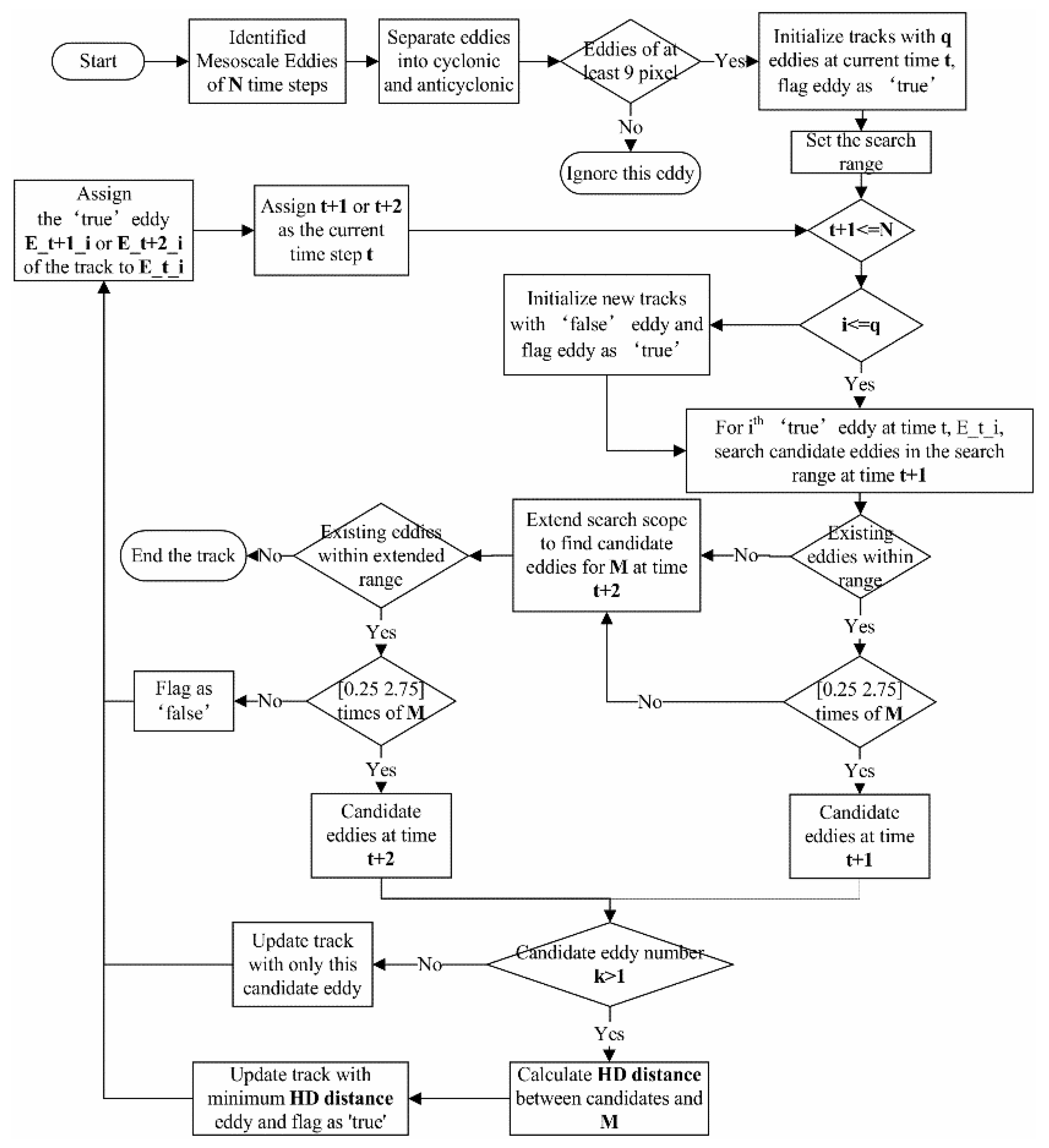
Initialization: Initialize the global eddy tracks using the eddy cores identified in the first time step, t.
(ii)
Searching: Search for each eddy at time t; then, search for the next candidate eddies in the next time step (t+1) within a specific range. The search area is an “ellipse” with a zonally oriented major axis. The western boundary of the ellipse is the distance from the eddy core, which is determined from the maximum value between 1.75 times the daily long Rossby wave propagation distance [41] and the mean mesoscale eddy propagation distance on the order of 10 km per day [42,43]. However, since 150 km was set as the minimum search range for weekly data by Chelton et al. [2] and we used daily data, the maximum daily travel distance of an eddy should be approximately 21 km. Furthermore, the altimeter data resolution is approximately 25 km; the eddy might “jump” or “disappear” because of sampling errors and measurement noise [2]. Thus, we extended the minimum search range of the western, eastern, southern and northern boundaries to 50 km.
(iii)
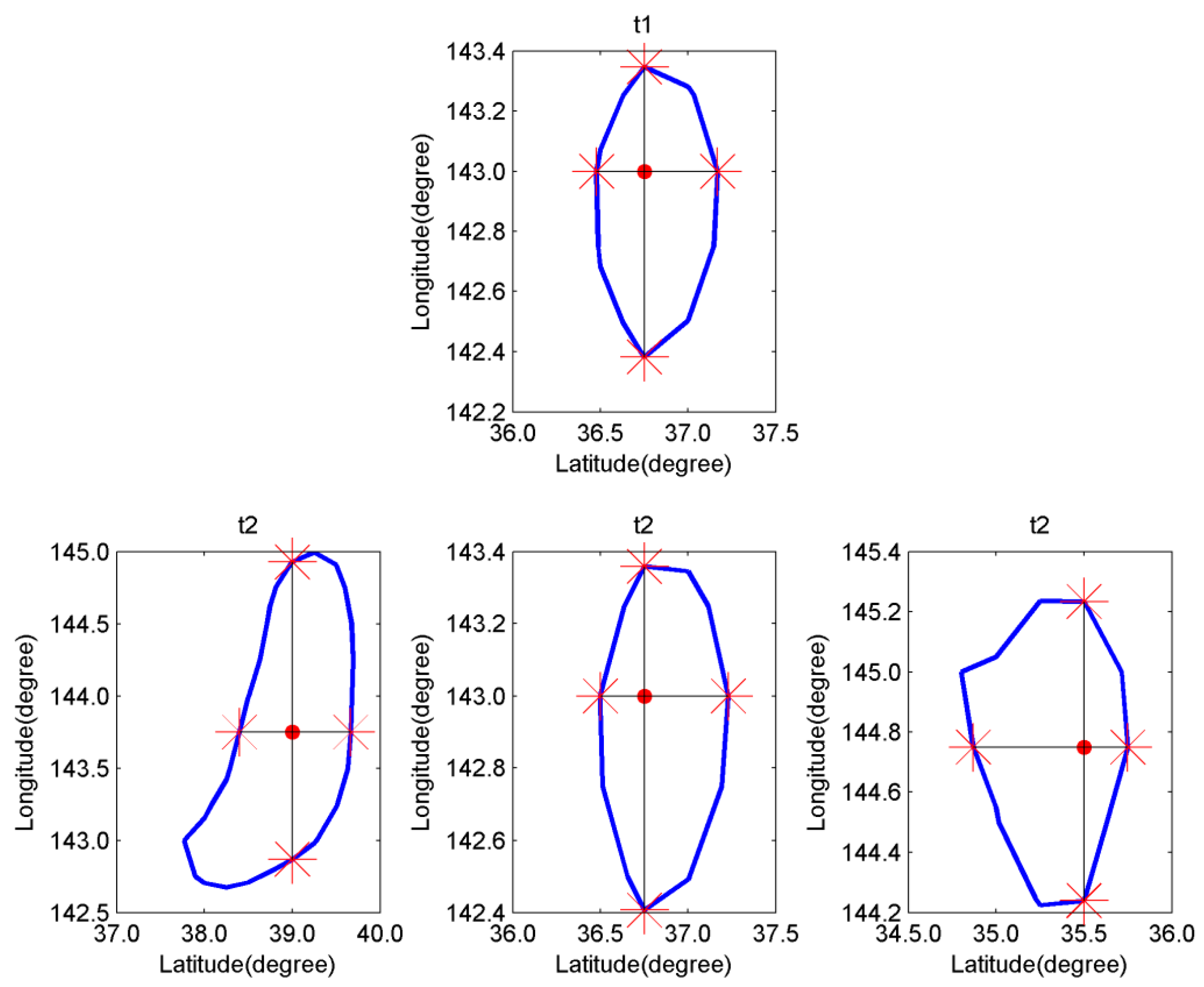
Selecting: After setting the search range, a selection procedure is carried out. Eddies within the search range at time step t+1 are candidate eddies if their area and amplitude are between 0.25 and 2.75 times those of the current eddy. When candidate eddies exist, the HD is calculated between the boundary of each candidate eddy and the current eddy boundary, and the candidate eddy with the minimum HD is selected as the next eddy. To account for the transient “disappearance” of the mesoscale eddies from the sea surface, we also allow eddies to “disappear” for one time step while tracking. Meanwhile, we expand the search area based on the propagation distance. Of course, we could perform the calculation using a larger number of time steps, but that is not the point of this paper. When no candidate eddy exists at time step t+1, a similar selection process is conducted at time step t+2 to find the next eddy. When no eligible eddy can be found at time step t+1 or t+2, the track of this eddy is stopped at time t. During this procedure, the selected eddy is flagged as true, while non-selected eddies are flagged as false.
(iv)
Updating: We update the recorded tracks at time t with the next selected eddies. Subsequently, if some eddies are still flagged as false at time t+1, then new tracks are initiated with each of these eddies, repeating the preceding steps to complete the long time series tracking of global eddies until the property limitations are exceeded.
For comparison, we also implemented the CH11 and similarity tracking methods for the same identified eddy dataset. To investigate the influences of eddy geometry, we also coded the CH11 and similarity tracking methods to allow eddies to “disappear” for one time step. Thus, the influence of a “disappearance” factor is excluded. Figure 3 shows the tracking results of the hybrid method for anticyclonic and cyclonic eddies.
The biggest difference between our tracking method and the other two methods (CH11 and similarity) lies in the selection of the next eddy. We take the experiment shown in the schematic diagram (Figure 4) as an example. The top single panel shows the current eddy at time t1, and the lower panels show three eddies that satisfy the area and amplitude criteria while searching nearby eddies during the next time step, t2. For CH11, the area and amplitude of nearby eddies match, and the first encountered eddy is selected if the two eddies have the same distance. This approach was also adopted by Faghmous et al. [33]. However, in this approach, the first selection depends on the loops in the routine instead of on the practical situation and may lead to a “jump” between eddy tracks. For the similarity method, it depends largely on the similarity of the physical properties of the eddies, whereas the proposed hybrid method considers the loose physical property limitations adopted from CH11 and the variation of the eddy boundary via HD. The HD distances between the t1 and t2 eddies were 2.97, 0.08, and 2.53. The result of this selection process is similar to that of “expert” tracking, and this process selects the middle eddy shown in the lower panels that has the smallest HD. Detailed comparison results are described in Section 3.

3. Global Long Time Series Comparison and Discussion
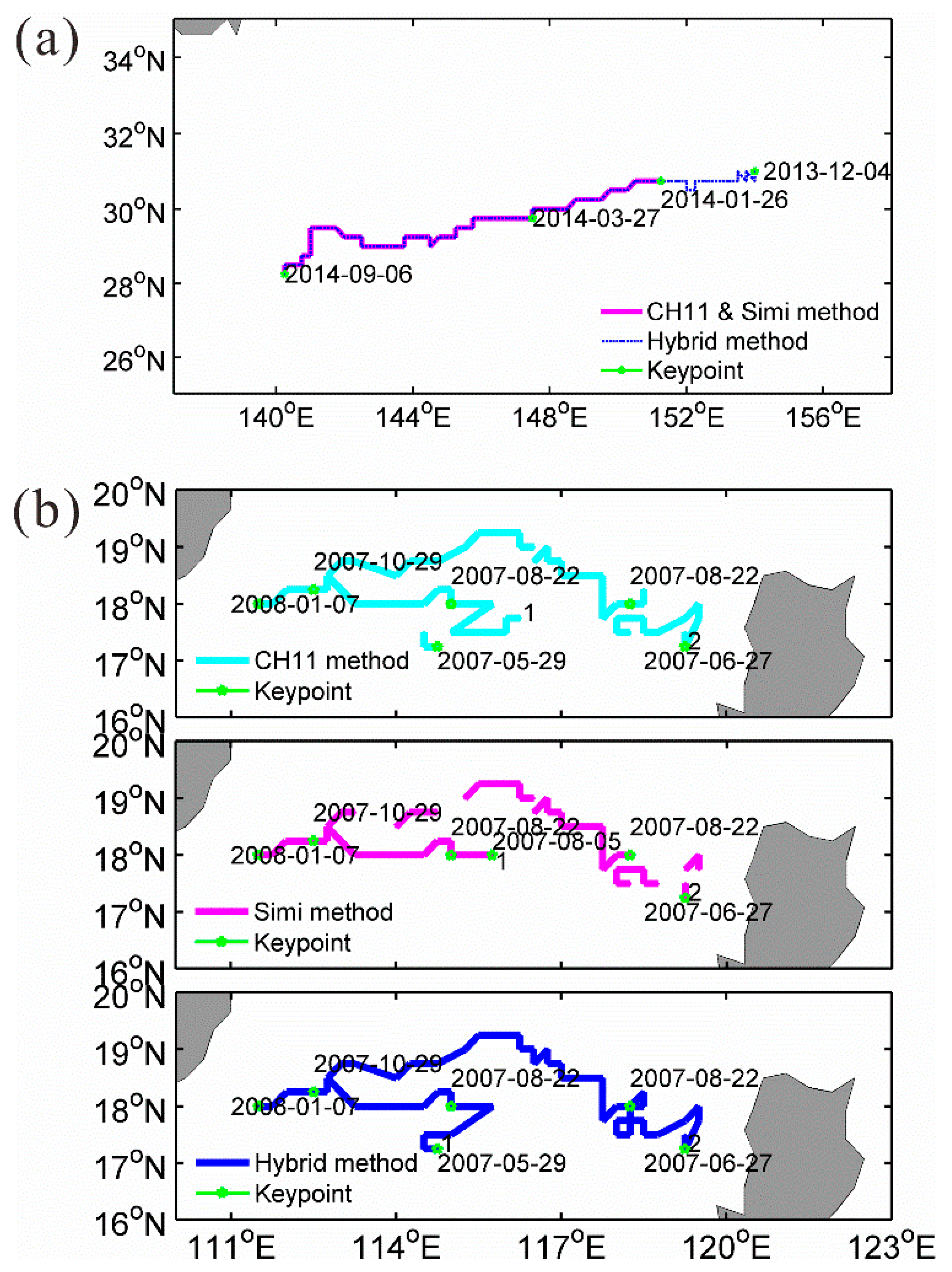
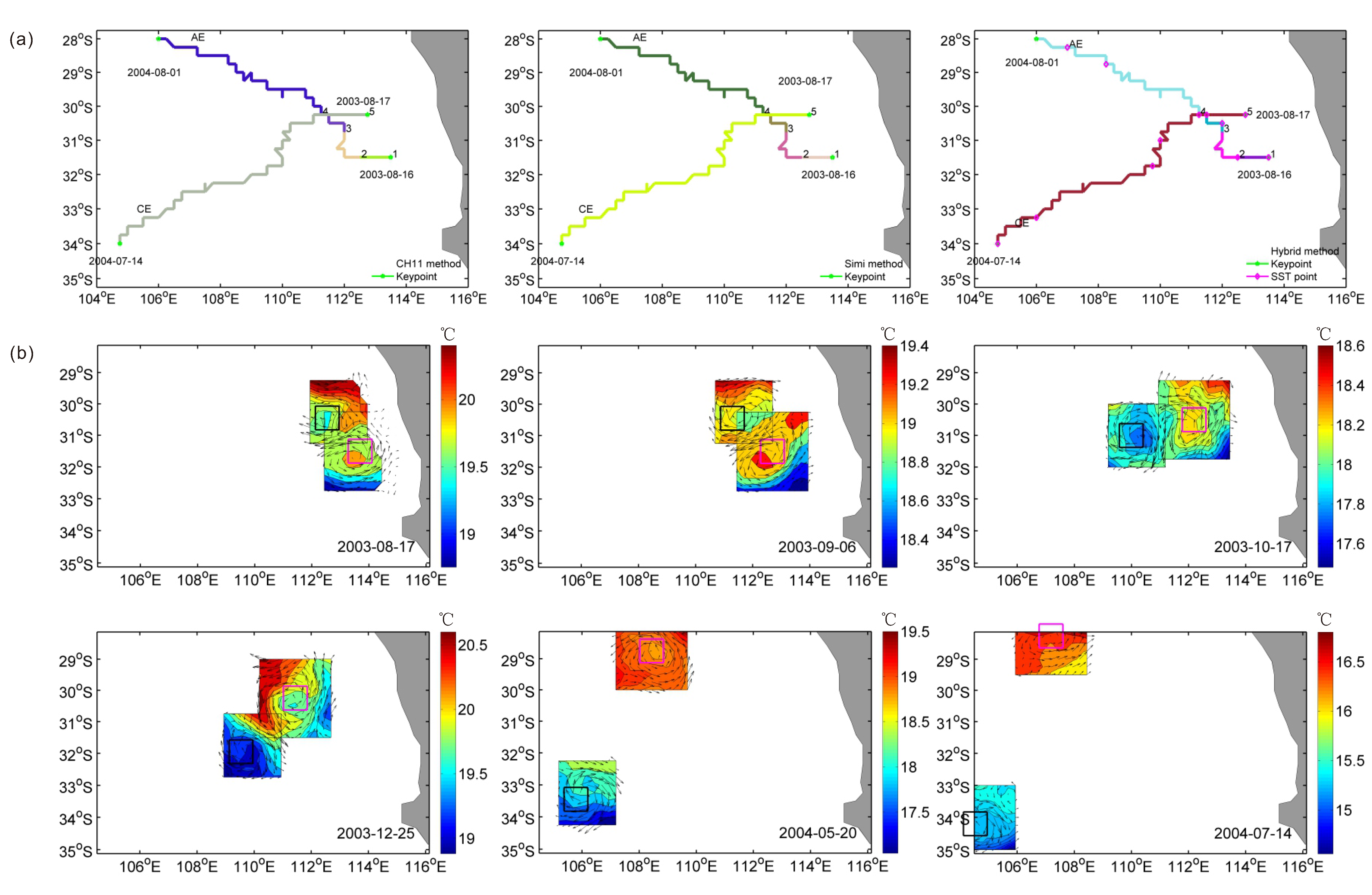
We tracked global mesoscale eddies with lifetimes longer than 10 days from 1993 to 2015 using three methods. Both the consistencies and discrepancies of the statistical results will be discussed in detail.
Table 1 shows the statistics for the detected eddy properties. We found that the values of the number, mean amplitude and rotational speed of cyclonic eddies are larger than those of anticyclonic eddies. In contrast, the values of the mean lifespan and radius of anticyclonic eddies are larger than those of cyclonic eddies. The discrepancies lie in the different values of the mean and maximum eddy properties tracked by the different methods. For instance, the hybrid method finds much longer-lived eddies, with a mean duration of approximately 31 days for cyclonic eddies and 32 days for anticyclonic eddies, while other methods indicate a duration of approximately 29 days for both cyclonic and anticyclonic eddies. The results from the three tracking methods show that the mean and maximum lifespans of anticyclonic eddies are longer than those of cyclonic eddies. The hybrid method results are more consistent with the mean and maximum results from the physical similarity method, which more reasonably selects the next candidate eddy.

3.1. Validation

Limited by the spatiotemporal resolution of satellite data, validation of eddy trajectories is performed in different ways. Some studies have reported paths inferred from sequential infrared imagery and drifting buoy trajectories [16,44], while some regional studies have compared the tracking results with “expert” visual results, as mentioned by Isern-Fontanet et al. [23].
In this paper, some reported eddies were used to validate the tracking results. Furthermore, SST and surface geostrophic currents (Equations (1)–(3)) were also adopted to further validate the tracking accuracy. Xu et al. [45] deployed 17 Argo floats to track an anticyclonic eddy from 27 March 2014 to 10 September 2014 in the North Pacific Ocean. Three tracking methods were applied to track this anticyclonic eddy. This specific eddy was also visually tracked by several “experts” as a comparison. In fact, visual inspection revealed that this eddy had existed since 4 December 2013. All three automatic algorithms could track this eddy. However, the hybrid method appeared to track the eddy for the longest period of time, as shown in Figure 5a. The CH11 and similarity methods achieved the same tracking results, tracking the eddy for 224 days, from 26 January 2014, to 6 September 2014. In contrast, as shown in the figure, the hybrid method tracked the eddy for 277 days, from 4 December 2013, to 6 September 2014 comparable to the visual tracking result. Figure 5b shows the eddies reported by Nan et al. [46] in the South China Sea, among which are two longer-lived eddies. These two eddies were generated on 5 August 2007, and 27 June 2007 and disappeared in January of 2008 and at the end of October of 2007 (tracks labelled 1 and 2), respectively. The algorithms had different performances in tracking these two eddies. The two traditional algorithms could achieve part-time tracking but regarded one eddy as several eddies, whereas the hybrid method could keep tracking of the eddy signals.
We detected an eddy off the west coast of the South Atlantic Ocean with a lifespan from early July to mid-December, 2006 (Figure 6). The existence of this eddy was further validated by the SST and surface geostrophic current field (Figure 6b). From the SST and current field, we can see that this eddy split into small-scale features on 21 September 2006 and finally merged into the background current on 12 December 2006. However, the hybrid method kept tracking signals as one main eddy maintaining its shape similar to the original eddy shape, while other methods regarded it as several eddies. The similarity method appears to be more vulnerable than the CH11 and hybrid methods, in mistakenly splitting one eddy into multiple smaller eddies during tracking (Figure 6a).
Another example involves eddies from the eastern South Pacific Ocean, as shown in Figure 7. Several eddies were tracked in this area from August 2003 to July 2004. All the algorithms detected these eddies and yielded the same result. Anticyclonic eddies and one cyclonic eddy in this area travelled equatorward and poleward. This divergent path of the anticyclonic and cyclonic eddies is a general feature of the world ocean and will be discussed in Section 3.3. The trajectories of the anticyclonic eddies consisted of different eddies that exceeded the amplitude or area limitation of the algorithm, although they were geographically connected. Additionally, note the SST patterns around the eddy centres in Figure 7b; the anticyclonic and cyclonic eddies last for a long time. SST along the anticyclonic eddy trajectories varies from time to time. The SST pattern also verifies that the anticyclonic eddies should not be considered as one eddy. In this eddy tracking example, the results of the hybrid method are comparable to those of the CH11 and similarity methods.
Overall, the hybrid method can track eddies for a longer period of time and detect eddy signals more robustly by taking the eddy boundary shape into consideration while tracking. Moreover, the hybrid method performed better when tracking splitting eddies.

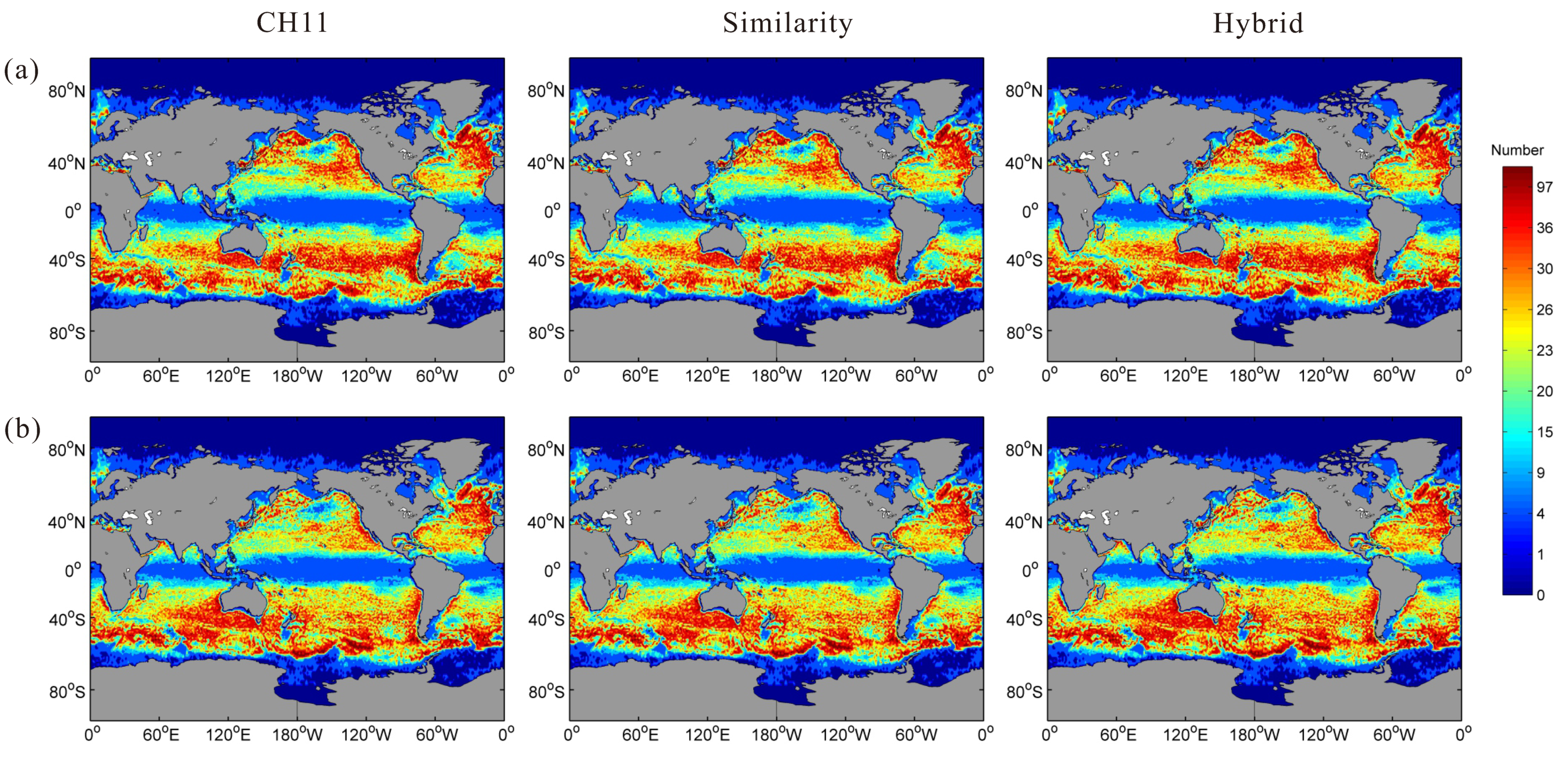
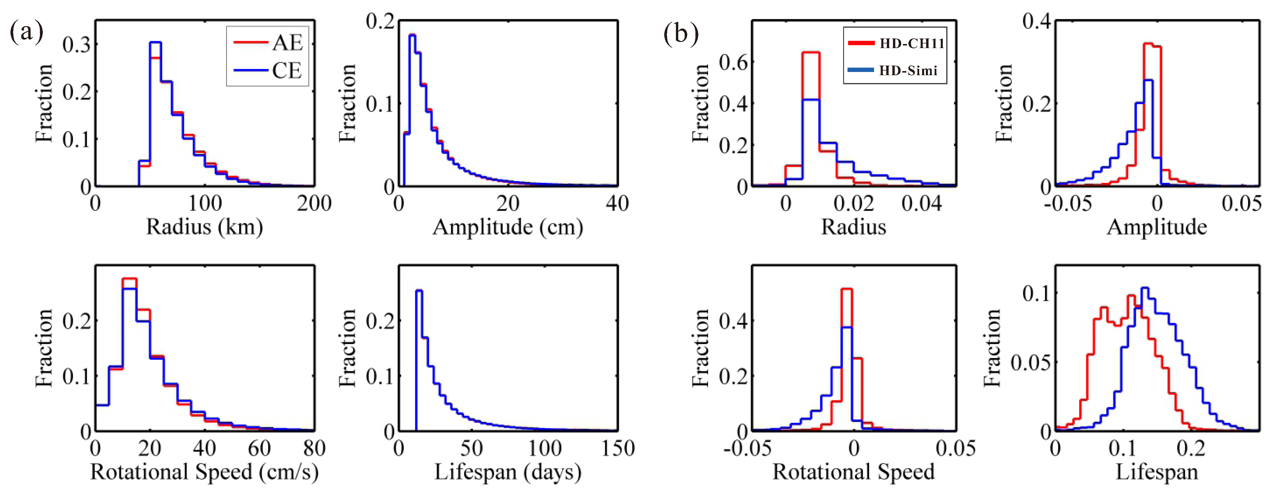
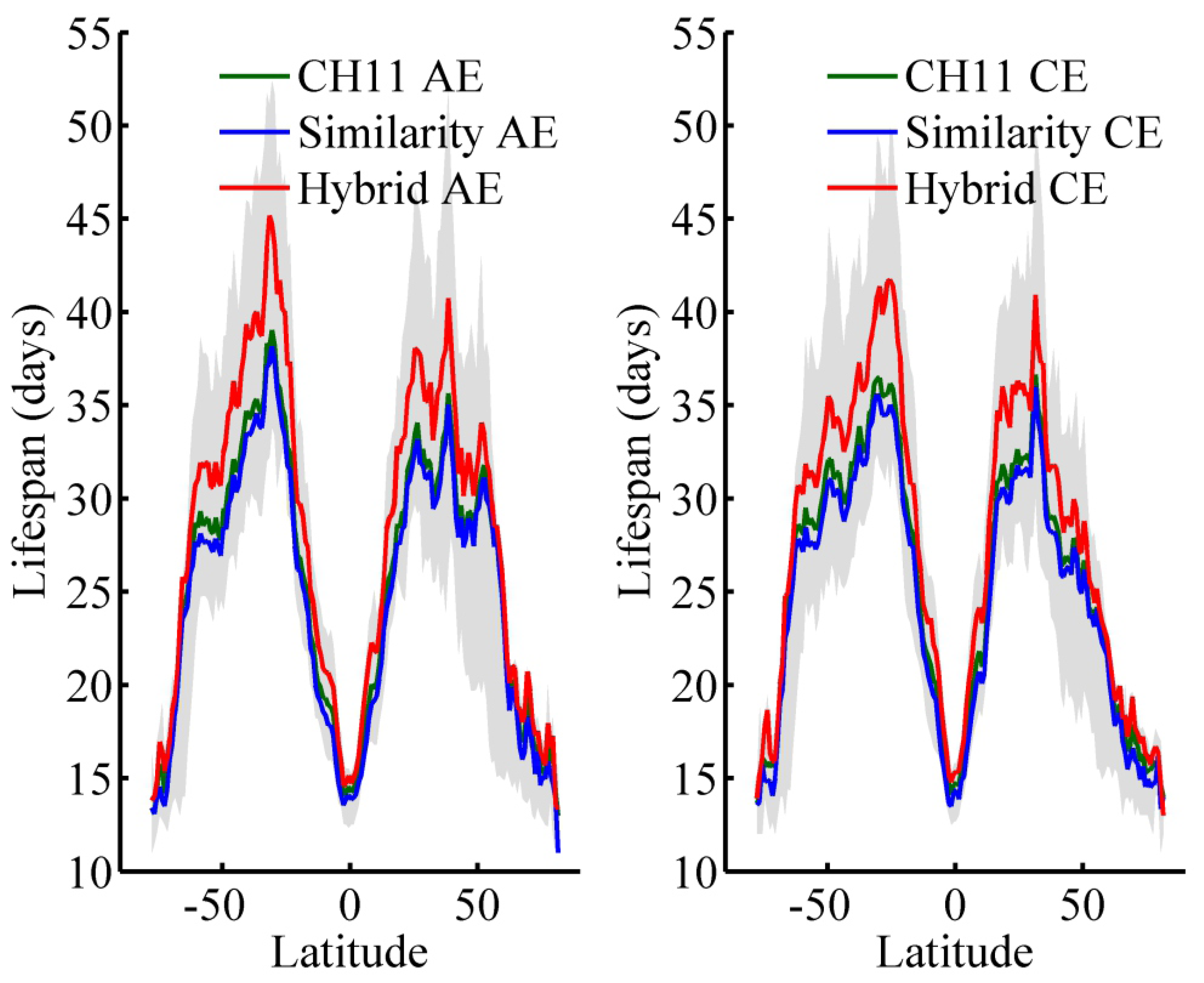
3.2. Eddy Frequency, Radius, Amplitude

Figure 8 presents the geographical distribution of the anticyclonic (Figure 8a) and cyclonic (Figure 8b) eddy frequency contained in the trajectories in each 1° × 1° region. The frequency of an eddy is the number of eddy occurrences along a track. The global distribution features from the three methods present similar eddy-rich areas located in the eastern North Pacific Ocean, eastern North Atlantic Ocean, Kuroshio Extension, Sea of Japan, and most parts of the Southern Ocean. These results have also been reported by Wooster and Reid [47], Chelton et al. [2], Heywood and Somayajulu [48], and Isoda [49]. The relative discrepancy, filtered by the Laplace filter between the hybrid and other methods, is shown in Figure 9. The hybrid method reveals greater eddy frequencies in most areas of the world oceans, but the relative differences are mostly within 5%. However, the hybrid method can track more eddy signals along trajectories in the equatorial and high-latitude areas because it considers variations in eddy shape.
The geographical distributions of the mean eddy properties are shown in Figure 10. The three methods show similar distributions of eddy properties. A clear large-scale distribution can be observed near the equator, where the radius reaches more than 200 km (Figure 10a,b). Large-amplitude eddy distributions are located in strong current areas, including the Kuroshio Current and its extension, the Gulf Stream and its extension, the Loop Current in the Gulf of Mexico, the Agulhas Current, the Agulhas Return Current, the Brazil–Malvinas Confluence Zone, the East Australia Current, the Antarctic Circumpolar Current and some areas near the Antarctic continent. These results are consistent with results by Chelton et al. [2]. The relative discrepancies in the radius and amplitude between the hybrid method and the other methods are small as shown in light green or light blue colours in Figure 11a,b. The differences in the average eddy radius and amplitude are 78.4 km and 10 cm, respectively. The differences are larger around the equator and in high-latitude regions, which may be related to the property distribution of the hybrid method averaged over the higher eddy occurrences in most areas of the ocean, especially in the equatorial and high-latitude regions.
Based on the geographical distribution of the consistencies and discrepancies between the three methods, histograms of the mean properties of eddies are shown separately for anticyclonic and cyclonic eddies in Figure 12a. Anticyclonic and cyclonic eddies show similar distributions. However, anticyclonic eddies have more large-scale signals than that of cyclonic eddies (here, “large-scale” refers to an eddy radius greater than 100 km). Approximately 98% of the mesoscale eddies have a radius smaller than 150 km, and approximately 70% have an amplitude less than 12 cm. Regarding the rotational speed, eddies with higher rotational speeds (higher than 25 cm/s) tend to be cyclonic. Most of the mesoscale eddies have a rotational speed of less than 40 cm/s. Approximately 90% of the eddy, either cyclonic or anticyclonic, have lifespans shorter than 50 days. Histograms of the relative differences are shown in Figure 12b for comparison. The relative differences in the radius, amplitude and rotational speeds derived from different methods are within 5%. However, the lifespan exhibits greater differences. According to the radius and lifespan, the hybrid method not only tracks eddies for longer durations but also preserves larger-scale eddy signals.

3.3. Propagation

The geographical distribution of the eddy rotational speed is shown in Figure 10c. High rotational speed eddies appear in the strong unstable current areas. The hybrid method produces a higher eddy rotational speed, an average of 92 cm/s higher (Figure 11c), in most areas, except in areas with strong currents such as the Kuroshio Current and its extension, the Antarctic circumpolar current region, the Gulf Stream and the Brazil–Malvinas confluence zone. Since unstable mesoscale eddies are difficult to track continuously, the consideration of the eddy boundary shape in the hybrid method tends to select the relatively stable signals whose properties vary less in this area. With less variation of eddy properties but with relatively more stable signals included in the strong current area of the hybrid method, the average property values will tend to be slightly smaller than those of other methods.
The lifespan distribution is calculated based on the birth location of each eddy and its track length. Therefore, we can closely inspect the generation sites where longer-lived eddies are produced. The lifespan distribution result plotted in Figure 10d shows the general variations. The relative differences in the lifespan distributions shown in Figure 11d indicate that the hybrid method tracks eddies with longer lifespans in most areas of the world oceans. The largest difference in the average eddy lifespan is 114 days. In addition, the CH11 and similarity methods show that approximately 88% of the eddy lifespans are shorter than 50 days, while the hybrid method derives smaller percentages. The ability of the hybrid method to perform continuous tracking is further illustrated by the mean latitudinal dependence, which is calculated by averaging the sum of the lifespan length over the eddy genesis number in each 1° latitude band (Figure 13). Steep growth is observed from high and low latitudes to the mid-latitudes.
Eddies with a lifespan equal to or longer than 16 weeks that crossed at least 10° longitudes were selected to investigate the propagation properties. There were 375, 291, and 736 anticyclonic and 452, 362, and 905 cyclonic eddies for the CH11, similarity, and hybrid methods. The chosen criterion was based on Chelton et al. [2] to obtain stable eddy signals. A composite analysis was performed by placing all the eddies at the same starting point (0, 0), as shown in Figure 14. Most eddies propagate westward, but the anticyclonic and cyclonic eddy trajectories apparently diverge. Cyclonic and anticyclonic eddies notably prefer poleward and equatorward trajectories, respectively. This observation was also mentioned by Morrow et al. [50] in their regional eddy study. The poleward deflection of cyclonic eddies was 73%, while the equatorward deflection was about 23% for the three methods. The equatorward deflections of the anticyclonic eddies were 85%, 87%, and 78%, and the poleward deflections were 12%, 10%, and 18% for the CH11, similarity, and hybrid tracking methods. The eddies propagate westward with meridional deflections caused by the β effect, which was confirmed by Morrow et al. [50]. When eddies rotate, they generate advection in the surrounding fluid in the same direction, leading small eddies toward the flanks of the large eddies. The combination of generated small eddies with a large eddy will result in meridional drift. Moreover, Early [51] mentioned that the finite spreads of the distributions of azimuths in the right column of Figure 14 may originate from eddy–eddy interactions. Beyond that, Chelton et al. [2] also mentioned that the influence of eddy–flow interactions might also cause the divergence of eddy paths.

3.4. EddySources and Sinks

Previous studies (e.g., Xu et al. [52] and Yang et al. [53]) have investigated eddy energy sources and sinks globally and regionally. In this study, we address the sources and sinks from the perspective of eddy numbers. The source of an eddy is defined as the starting of each eddy track. Similarly, the sink of an eddy is defined as the ending of each eddy track. Thus, the net eddy numbers can be calculated from the difference between 23 years’ worth of sources and sinks in each 1°× 1° region. The geographical distribution of the eddy sources and sinks based on the hybrid method is shown in Figure 15. Note that the eddy sources tend to be located along the eastern boundaries of ocean basins, whereas the eddy sinks are located close to the western boundaries of ocean basins. Xu et al. [52] mentioned that a high eddy energy generation/dissipation rate occurs along eastern boundaries and in regions with complex topography and current interactions. Most eddies propagate westward after being generated and then dissipate or transfer energy vertically into higher modes near the western boundary [2,22,54]. Our results are consistent with the above-mentioned literature results.

4. Conclusions

This paper proposed a hybrid method to automatically track global mesoscale eddies using identified mesoscale eddy datasets from 23 years of satellite altimeter data. The integration of both the physical and geometric properties of eddies was adopted to select the next eddies while tracking. We used Hausdorff distance (HD) to calculate the variations of eddy boundaries. The hybrid method improved the accuracy and the continuous tracking of eddies—even of splitting eddies. These results were validated by in situ eddy information datasets. In addition, our tracking results were geographically and statistically compared to those of other methods in terms of the eddy radius, amplitude, rotational speed and lifespan. Both the consistencies and discrepancies between the tested methods were discussed in detail. We found consistent geographical distributions among the methods in terms of the eddy radius, amplitude and rotational speed on a global scale. However, there were obvious discrepancies in the eddy lifespans, with relative differences of more than 10%. Based on the radius and lifespan data, the hybrid method not only tracks eddies longer but also maintains tracking of larger-scale eddy signals. The sources of eddies are along the eastern ocean boundaries, while the sinks of eddies are along the western boundaries. The lifespan distribution exhibited steep growth from high and low latitudes to middle latitudes. A clear divergent pathway shows that cyclonic eddies tend to travel poleward while anticyclonic eddies tend to travel equatorward. Our analysis shows that there are more cyclonic eddies than anticyclonic eddies in the world oceans.
The proposed hybrid method can provide technical support for in situ tracking and measurement of the structures of robust eddies. Furthermore, the generally consistent distribution of the tracking results could help discover the rules of mesoscale eddies. The limitations of this work are related to the lack of regional studies and comparisons for the investigation of specific regional eddy formation and propagation mechanisms. One issue is that the sampling quality of satellite altimeters in the AVISO SLA field may lead to inaccurate locations of eddy cores which may result in discontinuities of eddy trajectories and tracking errors. Due to the lack of additional in situ data, complete validation of the tracking results still requires further information.

Acknowledgments

The authors are grateful to the reviewers for their work and constructive comments. This research was jointly supported by the Natural Science Foundation of China under Grant No. U1406404, 41331172 and 61361136001, and the Scientific and Technological Innovation Project of the Qingdao National Laboratory for Marine Science and Technology under Grant No. 2015ASKJ01. The altimeter data were freely downloaded from the AVISO website (http://www.aviso.altimetry.fr/en/home.html).

Author Contributions

G.C. and F.T. conceived and designed the experiments; M.S. performed the experiments; M.S. and Y.L. analyzed the data; M.S. wrote the paper. G.C. and F.T. helped modify the manuscript.

Conflicts of Interest

The authors declare no conflict of interest.

References

  1. Bryden, H.L.; Brady, E.C. Eddy momentum and heat fluxes and their effects on the circulation of the equatorial Pacific Ocean. J. Mar. Res. 1989, 47, 55–79. [Google Scholar] [CrossRef]
  2. Chelton, D.B.; Schlax, M.G.; Samelson, R.M. Global observations of nonlinear mesoscale eddies. Prog. Oceanogr. 2011, 91, 167–216. [Google Scholar] [CrossRef]
  3. McGillicuddy, D.J.; Anderson, L.A.; Bates, N.R.; Bibby, T.; Buesseler, K.O.; Carlson, C.A.; Davis, C.S.; Ewart, C.; Falkowski, P.G.; Goldthwait, S.A.; et al. Eddy/wind interactions stimulate extraordinary mid-ocean plankton blooms. Science 2007, 316, 1021–1026. [Google Scholar] [CrossRef] [PubMed]
  4. Holloway, G. Estimation of oceanic eddy transports from satellite altimetry. Nature 1986, 323, 243–244. [Google Scholar] [CrossRef]
  5. McWilliams, J. Parameterizing eddy-induced tracer transports in ocean circulation models. J. Phys. Oceanogr. 1995, 25, 463–474. [Google Scholar]
  6. Stammer, D. On eddy characteristics, eddy transports, and mean flow properties. J. Phys. Oceanogr. 1998, 28, 727–739. [Google Scholar] [CrossRef]
  7. Morrow, R.; Fang, F.; Fieux, M.; Molcard, R. Anatomy of three warm-core Leeuwin Current eddies. Deep Sea Res. Part II Top. Stud. Oceanogr. 2003, 50, 2229–2243. [Google Scholar] [CrossRef]
  8. Volkov, D.L.; Lee, T.; Fu, L.L. Eddy-induced meridional heat transport in the ocean. Geophys. Res. Lett. 2008, 35. [Google Scholar] [CrossRef]
  9. Early, J.J.; Samelson, R.; Chelton, D.B. The evolution and propagation of quasigeostrophic ocean Eddies. J. Phys. Oceanogr. 2011, 41, 1535–1555. [Google Scholar] [CrossRef]
  10. Krauß, W.; Böning, C.W. Lagrangian properties of eddy fields in the northern North Atlantic as deduced from satellite-tracked buoys. J. Mar. Res. 1987, 45, 259–291. [Google Scholar] [CrossRef] [Green Version]
  11. Pingree, R. Winter warming in the southern Bay of Biscay and Lagrangian eddy kinematics from a deep-drogued Argos buoy. J. Mar. Biol. Assoc. UK 1994, 74, 107–128. [Google Scholar] [CrossRef]
  12. Crawford, W.R.; Whitney, F.A. Mesoscale eddy aswirl with data in Gulf of Alaska. Eos Trans. Am. Geophys. Union 1999, 80, 365–370. [Google Scholar] [CrossRef]
  13. Sadarjoen, I.A.; Post, F.H. Detection, quantification, and tracking of vortices using streamline geometry. Comput. Graph. 2000, 24, 333–341. [Google Scholar] [CrossRef]
  14. Wade, I.P.; Heywood, K.J. Tracking the PRIME eddy using satellite altimetry. Deep Sea Res. Part II Top. Stud. Oceanogr. 2001, 48, 725–737. [Google Scholar] [CrossRef]
  15. Puillat, I.; Letage, I.T.; Millot, C. Algerian eddies lifetime can near 3 years. J. Mar. Syst. 2002, 31, 245–259. [Google Scholar] [CrossRef]
  16. Fontanet, J.I.; Ladona, E.G.; Font, J. Identification of marine eddies from altimetric maps. J. Atmos. Ocean. Technol. 2003, 20, 772–778. [Google Scholar] [CrossRef]
  17. Penven, P.; Echevin, V.; Pasapera, J.; Colas, F.; Tam, J. Average circulation, seasonal cycle, and mesoscale dynamics of the Peru Current System: A modeling approach. J. Geophys. Res. Oceans 2005, 110. [Google Scholar] [CrossRef]
  18. Chaigneau, A.; Gizolme, A.; Grados, C. Mesoscale eddies off Peru in altimeter records: Identification algorithms and eddy spatio-temporal patterns. Prog. Oceanogr. 2008, 79, 106–119. [Google Scholar] [CrossRef]
  19. Chaigneau, A.; Eldin, G.; Dewitte, B. Eddy activity in the four major upwelling systems from satellite altimetry (1992–2007). Prog. Oceanogr. 2009, 83, 117–123. [Google Scholar] [CrossRef]
  20. Chen, G.; Hou, Y.; Chu, X. Mesoscale eddies in the South China Sea: Mean properties, spatiotemporal variability, and impact on thermohaline structure. J. Geophys. Res. Oceans 2011, 116. [Google Scholar] [CrossRef]
  21. Mason, E.; Pascual, A.; McWilliams, J.C. A new sea surface height–based code for oceanicmesoscale eddy tracking. J. Atmos. Ocean. Technol. 2014, 31, 1181–1188. [Google Scholar] [CrossRef]
  22. Chelton, D.B.; Schlax, M.G.; Samelson, R.M.; de Szoeke, R.A. Global observations of large oceanic eddies. Geophys. Res. Lett. 2007, 34. [Google Scholar] [CrossRef]
  23. Fontanet, J.I.; Ladona, E.G.; Font, J. Vortices of the Mediterranean Sea: An altimetric perspective. J. Phys. Oceanogr. 2006, 36, 87–103. [Google Scholar] [CrossRef]
  24. Doglioli, A.; Blanke, B.; Speich, S.; Lapeyre, G. Tracking coherent structures in a regional ocean model with wavelet analysis: Application to Cape Basin eddies. J. Geophys. Res. Oceans 2007, 112. [Google Scholar] [CrossRef]
  25. Xiu, P.; Chai, F.; Shi, L.; Xue, H.; Chao, Y. A census of eddy activities in the South China Sea during 1993–2007. J. Geophys. Res. Oceans 2010, 115. [Google Scholar] [CrossRef]
  26. Fontanet, J.I.; Lapeyre, G.; Klein, P.; Chapron, B.; Hecht, M.W. Three-dimensional reconstruction of oceanic mesoscale currents from surface information. J. Geophys. Res. Oceans 2008, 113. [Google Scholar] [CrossRef]
  27. Chaigneau, A.; Le Texier, M.; Eldin, G.; Grados, C.; Pizarro, O. Vertical structure of mesoscale eddies in the eastern South Pacific Ocean: A composite analysis from altimetry and Argo profiling floats. J. Geophys. Res. Oceans 2011, 116. [Google Scholar] [CrossRef]
  28. Dong, C.; Lin, X.; Liu, Y.; Nencioli, F.; Chao, Y.; Guan, Y.; Chen, D.; Dickey, T.; McWilliams, J.C. Three-dimensional oceanic eddy analysis in the Southern California Bight from a numerical product. J. Geophys. Res. Oceans 2012, 117. [Google Scholar] [CrossRef]
  29. Yang, G.; Wang, F.; Li, Y.; Lin, P. Mesoscale eddies in the northwestern subtropical Pacific Ocean: Statistical characteristics and three-dimensional structures. J. Geophys. Res. Oceans 2013, 118, 1906–1925. [Google Scholar] [CrossRef]
  30. Lin, X.; Dong, C.; Chen, D.; Liu, Y.; Yang, J.; Zou, B.; Guan, Y. Three-dimensional properties of mesoscale eddies in the South China Sea based on eddy-resolving model output. Deep Sea Res. Part I Oceanogr. Res. Pap. 2015, 99, 46–64. [Google Scholar] [CrossRef]
  31. Nencioli, F.; Dong, C.; Dickey, T.; Washburn, L.; McWilliams, J.C. A vector geometry-based eddy detection algorithm and its application to a high-resolution numerical model product and high-frequency radar surface velocities in the Southern California Bight. J. Atmos. Ocean. Technol. 2010, 27, 564–579. [Google Scholar] [CrossRef]
  32. Kurczyn, J.; Beier, E.; Lavín, M.; Chaigneau, A. Mesoscale eddies in the northeastern Pacific tropical-subtropical transition zone: Statistical characterization from satellite altimetry. J. Geophys. Res. Oceans 2012, 117. [Google Scholar] [CrossRef] [Green Version]
  33. Faghmous, J.H.; Frenger, I.; Yao, Y.; Warmka, R.; Lindell, A.; Kumar, V. A daily global mesoscale ocean eddy dataset from satellite altimetry. Sci. Data 2015, 2. [Google Scholar] [CrossRef] [PubMed]
  34. AVISO. SSALTO/DUACS User Handbook: (M) SLA and (M) ADT Near-Real Time and Delayed Time Products. Available online: http://www.aviso.altimetry.fr/fileadmin/documents/data/tools/hdbk_duacs.pdf (accessed on 23 February 2017).
  35. Remote Sensing Systems. Available online: http://www.remss.com/measurements/sea-surface-temperature (accessed on 23 February 2017).
  36. Liu, Y.; Chen, G.; Sun, M.; Tian, F. A Parallel SLA-Based Algorithm for Global Mesoscale Eddy Identification. J. Atmos. Ocean. Technol. 2016, 33, 2743–2754. [Google Scholar] [CrossRef]
  37. Segond, M. Algorithmes Bio-mimétiques pour la Reconnaissance de Formesetl’apprentissage. Ph.D. Thesis, Universite du Littoral, Calais, France, 8 December 2006. [Google Scholar]
  38. De Carvalho, F.D.A.; de Souza, R.M.; Chavent, M.; Lechevallier, Y. Adaptive Hausdorff distances and dynamic clustering of symbolic interval data. Pattern Recognit. Lett. 2006, 27, 167–179. [Google Scholar] [CrossRef]
  39. Huttenlocher, D.P.; Klanderman, G.A.; Rucklidge, W.J. Comparing images using the Hausdorff distance. IEEE Trans. Pattern Anal. Mach. Intell. 1993, 15, 850–863. [Google Scholar] [CrossRef]
  40. Qiang, H.Q.; Qian, C.H.; Gong, S.R. Similarity Measure for Image Retrieval Based on Hausdorff Distance. In Applied Mechanics and Materials; Trans Tech Publications: Zurich, Switzerland, 2014; Volume 635, pp. 1039–1044. [Google Scholar]
  41. Chelton, D.B.; Deszoeke, R.A.; Schlax, M.G.; El Naggar, K.; Siwertz, N. Geographical variability of the first baroclinic Rossby radius of deformation. J. Phys. Oceanogr. 1998, 28, 433–460. [Google Scholar] [CrossRef]
  42. Lentini, C.A.; Olson, D.B.; Podestá, G.P. Statistics of Brazil Current rings observed from AVHRR: 1993 to 1998. Geophys. Res. Lett. 2002, 29. [Google Scholar] [CrossRef]
  43. Zhang, W.Z.; Xue, H.; Chai, F.; Ni, Q. Dynamical processes within an anticyclonic eddy revealed from Argo floats. Geophys. Res. Lett. 2015, 42, 2342–2350. [Google Scholar] [CrossRef]
  44. Font, J.; Isert-Fontanet, J.; De Jesus Salas, J. Tracking a big anticyclonic eddy in the western Mediterranean Sea. Sci. Mar. 2004, 68, 331–342. [Google Scholar] [CrossRef]
  45. Xu, L.; Li, P.; Xie, S.P.; Liu, Q.; Liu, C.; Gao, W. Observing mesoscale eddy effects on mode-water subduction and transport in the North Pacific. Nat. Commun. 2016, 7. [Google Scholar] [CrossRef] [PubMed]
  46. Nan, F.; He, Z.; Zhou, H.; Wang, D. Three long-lived anticyclonic eddies in the northern South China Sea. J. Geophys. Res. Oceans 2011, 116. [Google Scholar] [CrossRef]
  47. Wooster, W.S.; Reid, J. Eastern boundary currents. Sea 1963, 2, 253–280. [Google Scholar]
  48. Heywood, K.J.; Somayajulu, Y.K. Eddy activity in the South Indian Ocean from ERS-1 altimetry. In Proceedings of the Third ERS Symposium on Space at the service of our Environment, Florence, Italy, 14–21 March 1997.
  49. Isoda, Y. Interaction of a warmeddy with the coastal current at the eastern boundary area in the Tsushima Current region. Cont. Shelf Res. 1996, 16, 1149–1163. [Google Scholar] [CrossRef]
  50. Morrow, R.; Birol, F.; Griffin, D.; Sudre, J. Divergent pathways of cyclonic and anti-cyclonic ocean eddies. Geophys. Res. Lett. 2004, 31. [Google Scholar] [CrossRef]
  51. Early, J.J. Mathematical Approaches to the Physics of Mesoscale Oceanography. Ph.D. Thesis, Oregon State University, 22 October 2009. [Google Scholar]
  52. Xu, C.; Shang, X.D.; Huang, R.X. Estimate of eddy energy generation/dissipation rate in the world ocean from altimetry data. Ocean Dyn. 2011, 61, 525–541. [Google Scholar] [CrossRef]
  53. Yang, H.; Wu, L.; Liu, H.; Yu, Y. Eddy energy sources and sinks in the South China Sea. J. Geophys. Res. Oceans 2013, 118, 4716–4726. [Google Scholar] [CrossRef]
  54. Zhai, X.; Johnson, H.L.; Marshall, D.P.; Wunsch, C. On the wind power input to the ocean general circulation. J. Phys. Oceanogr. 2012, 42, 1357–1365. [Google Scholar] [CrossRef]
Figure 1. Geographical distribution of the identified (a) anticyclonic and (b) cyclonic eddy signals in each 1° × 1° region over a period of 23 years from 1993 to 2015.
Remotesensing 09 00206 g001
Figure 2. Hybrid algorithm workflow.
Remotesensing 09 00206 g002
Figure 3. Geographical distribution of long-lived (longer than 16 weeks) (a) Anticyclonic and (b) Cyclonic eddytracks identifiedusing the hybrid method over a period of 23 years from 1993 to 2015.
Remotesensing 09 00206 g003
Figure 4. Example eddy at the t1 time step and its candidate eddies at the t2 time step.
Remotesensing 09 00206 g004
Figure 5. (a) For a reported Western Pacific eddy, the CH11 and similarity methods produce the same track (magenta line), while the hybrid method tracks the eddy for a longer period of time (blue dotted line). The green star denotesthe milestone points along the track. The dates are as follows: “2013-12-04” denotes where and when this eddy formed and the beginning of the hybrid method tracking,“2014-01-26” denotes the point at which the CH11 and similarity tracking began,“2014-03-27” denotes where and when the 17 Argo floats were deployed, and “2014-09-06” denotes when and where the tracking ended; (b) Tracking results of the three algorithms for eddies reported in the South China Sea. Numbers “1” and “2” represent two eddies named Eddy1 and Eddy2. Eddy1 was tracked using the hybrid method from “2007-05-29” to “2007-10-29”, and Eddy2 was tracked from“2007-06-27” to “2008-01-07”. This result is consistent with former validated work. The other two methods resulted in different tracks along the eddy paths.
Remotesensing 09 00206 g005
Figure 6. (a) Anticyclonic eddy off the west coast of the South Atlantic Ocean tracked using three methods (CH11, similarity and hybrid methods, from left to right) in 2006; (b) SST and geostrophic current field extracted from the eddy region. This eddy splits into two parts while propagating. Only the hybrid method could tolerate the split and continue tracking it using the major feature of the “mother” eddy.
Remotesensing 09 00206 g006
Figure 7. Two eddies tracked in the eastern South Pacific Ocean from August 2003, to August 2004. (a) Tracking paths from the three methods; (b) Corresponding SST and geostrophic current field along the trajectory of the hybrid method.
Remotesensing 09 00206 g007
Figure 8. Comparison of the geographical distribution of (a) Anticyclonic and (b) Cyclonic eddy frequencies along eddy trajectories determined using the three tracking methods in each 1° × 1° region.
Remotesensing 09 00206 g008
Figure 9. Relative differences between the geographical distributions of (a) anticyclonic and (b) cyclonic eddies determined using the hybrid and CH11 methods (left column) and using the hybrid and similarity methods (right column) in each 1° × 1° region.
Remotesensing 09 00206 g009
Figure 10. Average eddy properties, including the (a) radius (km); (b) amplitude (cm); (c) rotational speed (cm/s) and (d) lifespan (days), for eddies with lifespans longer than 10 days for each 1° × 1° region from(from left to right) the CH11, similarity and hybrid methods.
Remotesensing 09 00206 g010
Figure 11. Relative differences in the average eddy properties of (a) radius (km); (b) amplitude (cm); (c) rotational speed (cm/s) and (d) lifespan (days) between the hybrid and CH11 methods and the hybrid and similarity methods(left to right)for eddies with lifespans longer than 10 days in each 1° × 1° region.
Remotesensing 09 00206 g011
Figure 12. (a) Global eddy statistics for cyclonic (CE) and anticyclonic (AE) eddies tracked by the hybrid method; (b) Relative difference between the hybrid and CH11 methods and the hybrid and similarity methods.
Remotesensing 09 00206 g012
Figure 13. Meridional profiles of the average (solid lines) eddy lifespans (in days) as tracked by the three methods and the interquartile range of the distribution from the hybrid method (grey shading) in 1° latitude bands.
Remotesensing 09 00206 g013
Figure 14. Meridional deflections of anticyclonic (left column panels) and cyclonic (middlecolumn panels) eddies with lifetimes longer than 16 weeks that propagated westward for a minimum of 10° longitude based on the three methods: (a) CH11; (b) Similarity and (c) Hybrid. The left and middle panels show the changes in longitude (negative westward) and latitude (positive for poleward and negative for equatorward due west) relative to the (0, 0) location for anticyclonic and cyclonic eddies. The right panels show histograms of the average azimuth of each eddy trajectory, defined in the left and middle columns. The labels in the right panels indicate the percentages of negative (left) and positive (right) eddy azimuths.
Remotesensing 09 00206 g014
Figure 15. Geographical distribution of the sources and sinks of eddies with lifespans longer than 10 days tracked by the hybrid method in each 1° × 1° region.
Remotesensing 09 00206 g015
Table 1. Properties of eddies with lifespans longer than 10 days obtained using the three tracking algorithms.
Tracking MethodTrack NumberMean Lifespan (Days)Max Lifespan (Days)Mean Amplitude (cm)Max Amplitude (cm)Mean Radius (km)Max Radius (km)Mean Rotational Speed (cm/s)Max Rotational Speed (cm/s)
CH11_CE552,31028.78535.598.467.0246.616.2162.5
CH11_AE537,75328.99405.296.169.4293.315.4157.1
Simi_CE552,21728.78535.978.168.8245.916.6150.8
Simi_AE537,63228.99405.678.071.8274.915.8109.0
Hybrid_CE528,91631.311135.878.069.0234.616.5150.8
Hybrid_AE512,44431.711625.569.272.0274.215.7106.0

