
A New Approach for Realistic 3D Reconstruction of Planar Surfaces from Laser Scanning Data and Imagery Collected Onboard Modern Low-Cost Aerial Mapping Systems


Abstract
: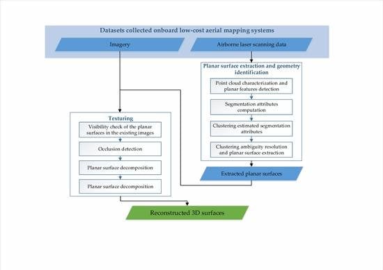
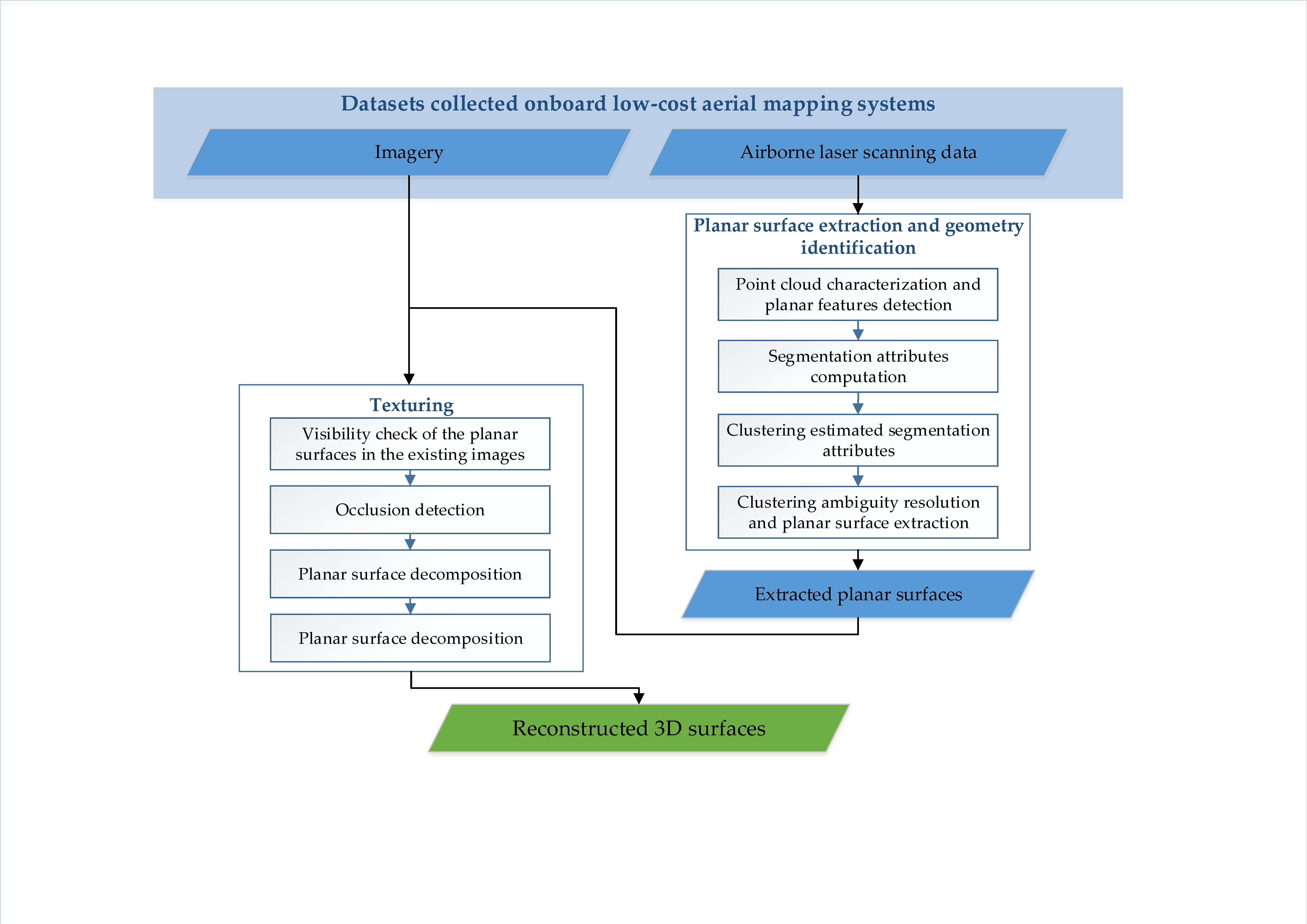
1. Introduction
2. Laser Scanning Data Segmentation and Planar Feature Extraction
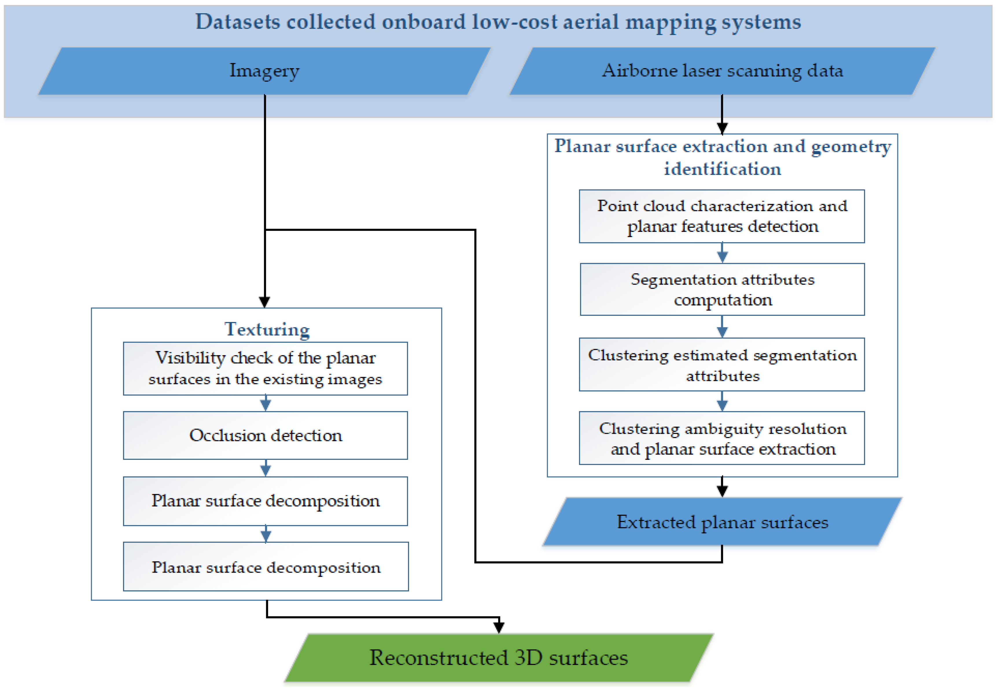
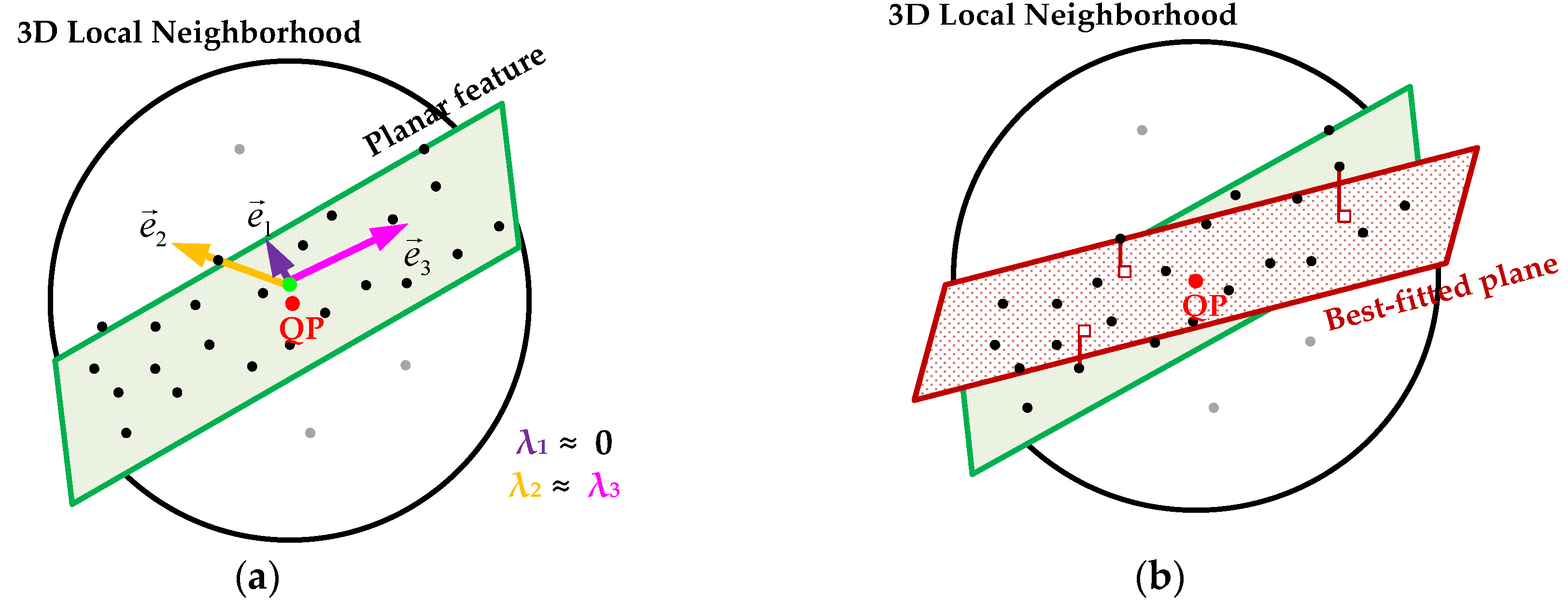
2.1. Point Cloud Characterization and Planar Features Detection
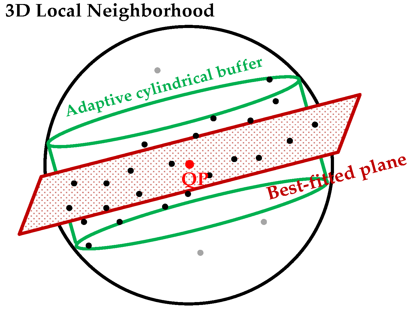
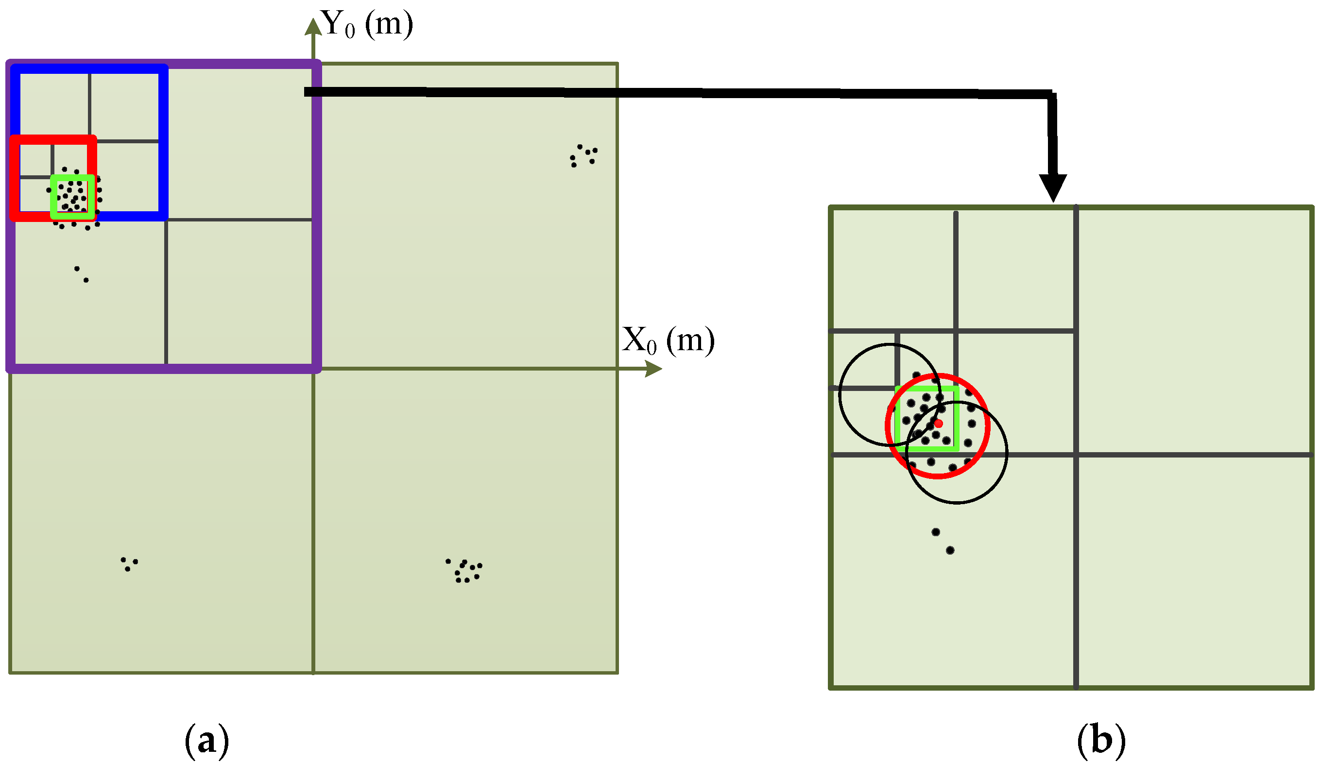
2.2. Segmentation Attributes Computation
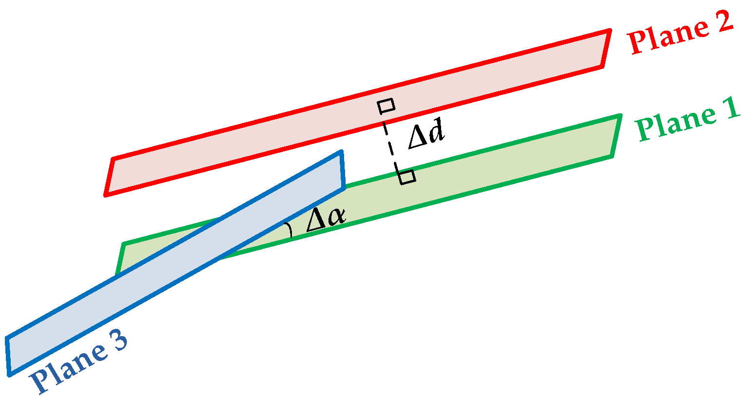
2.3. Clustering of the Estimated Attributes and Segmentation of Planar Surfaces
3. Texturing of Extracted Planar Surfaces from Laser Scanning Data
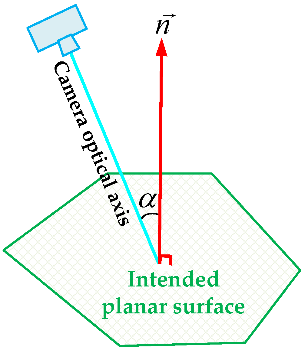
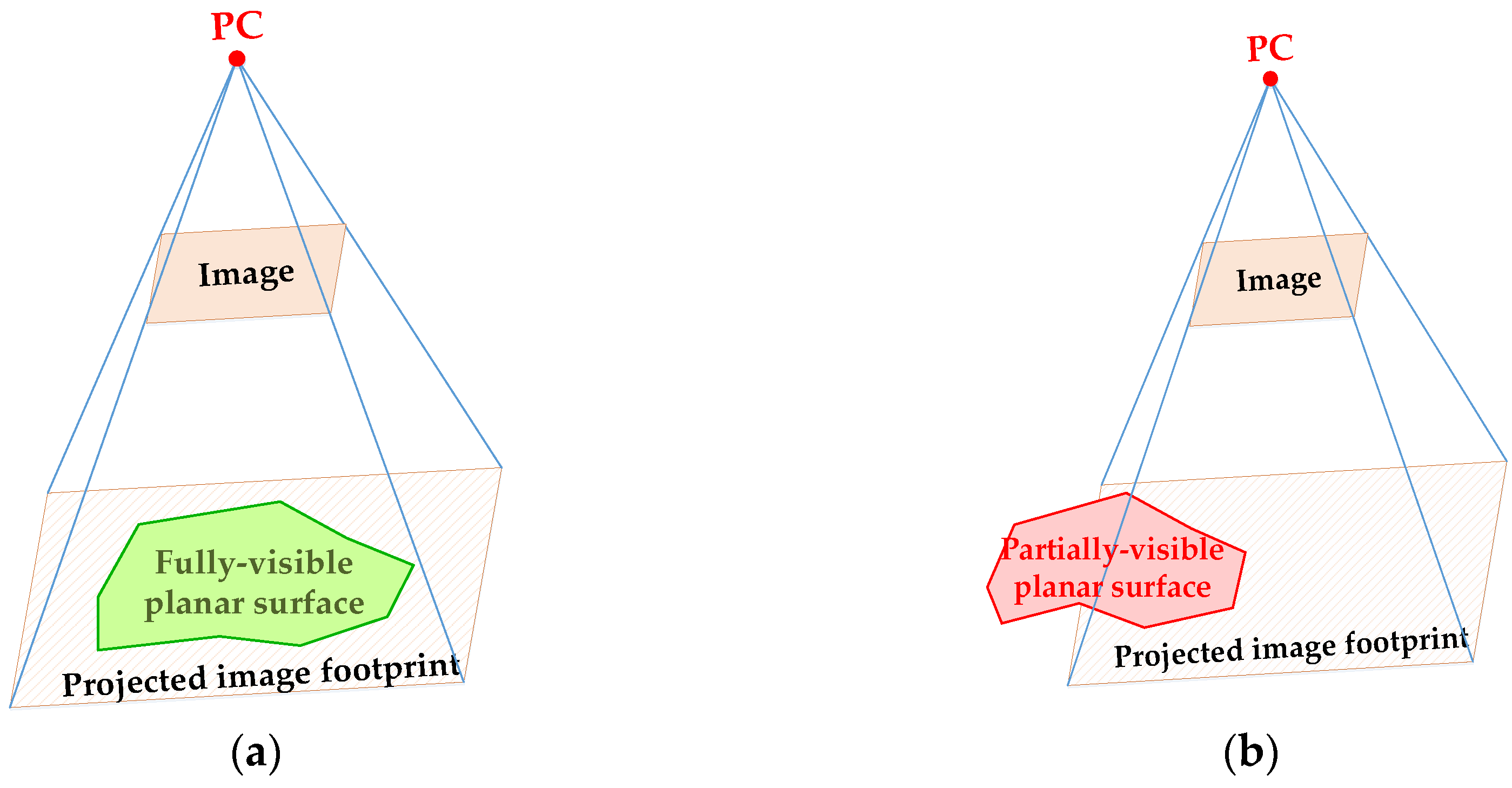
3.1. Visibility Check
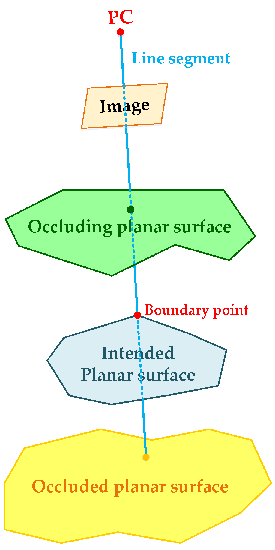
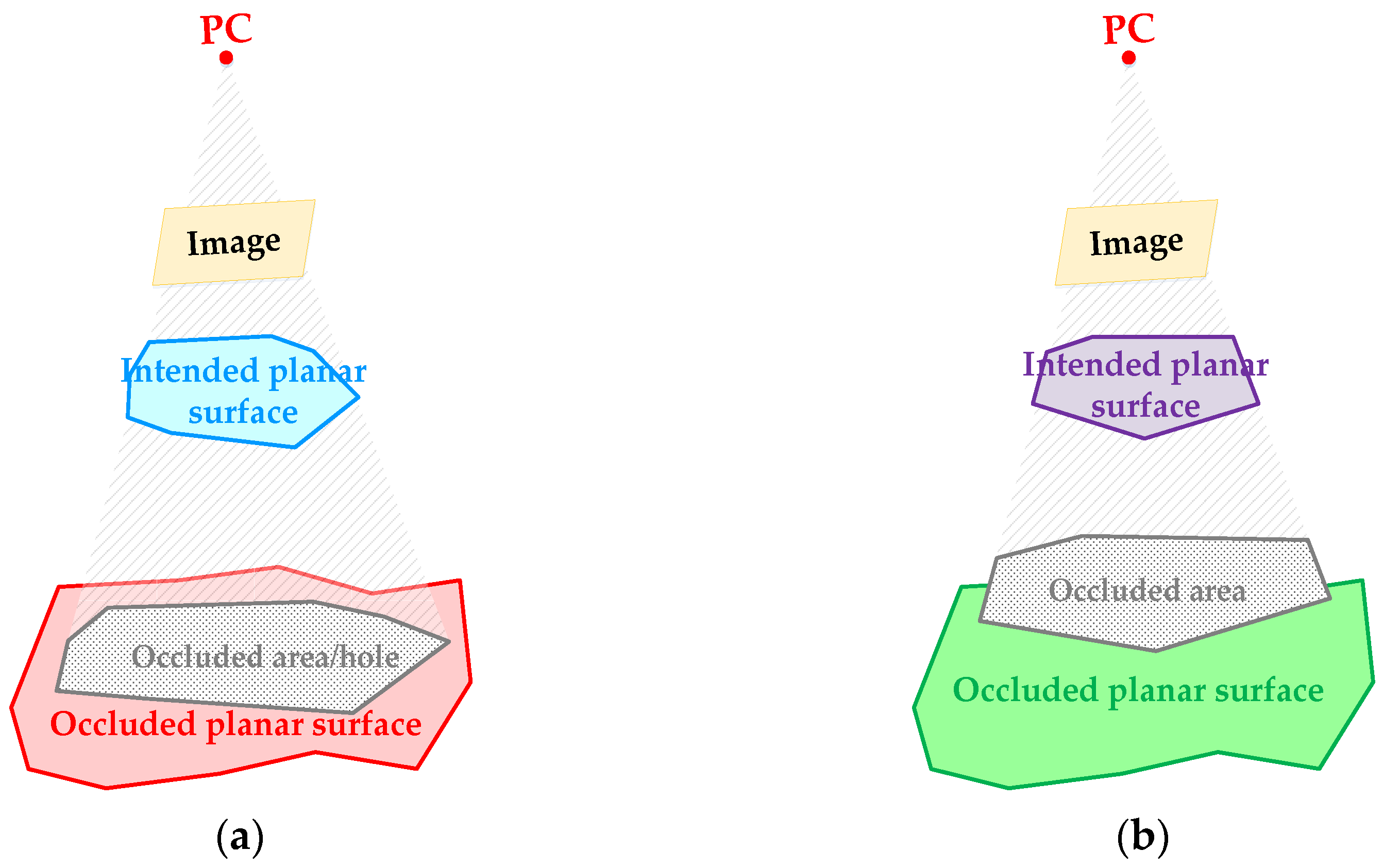
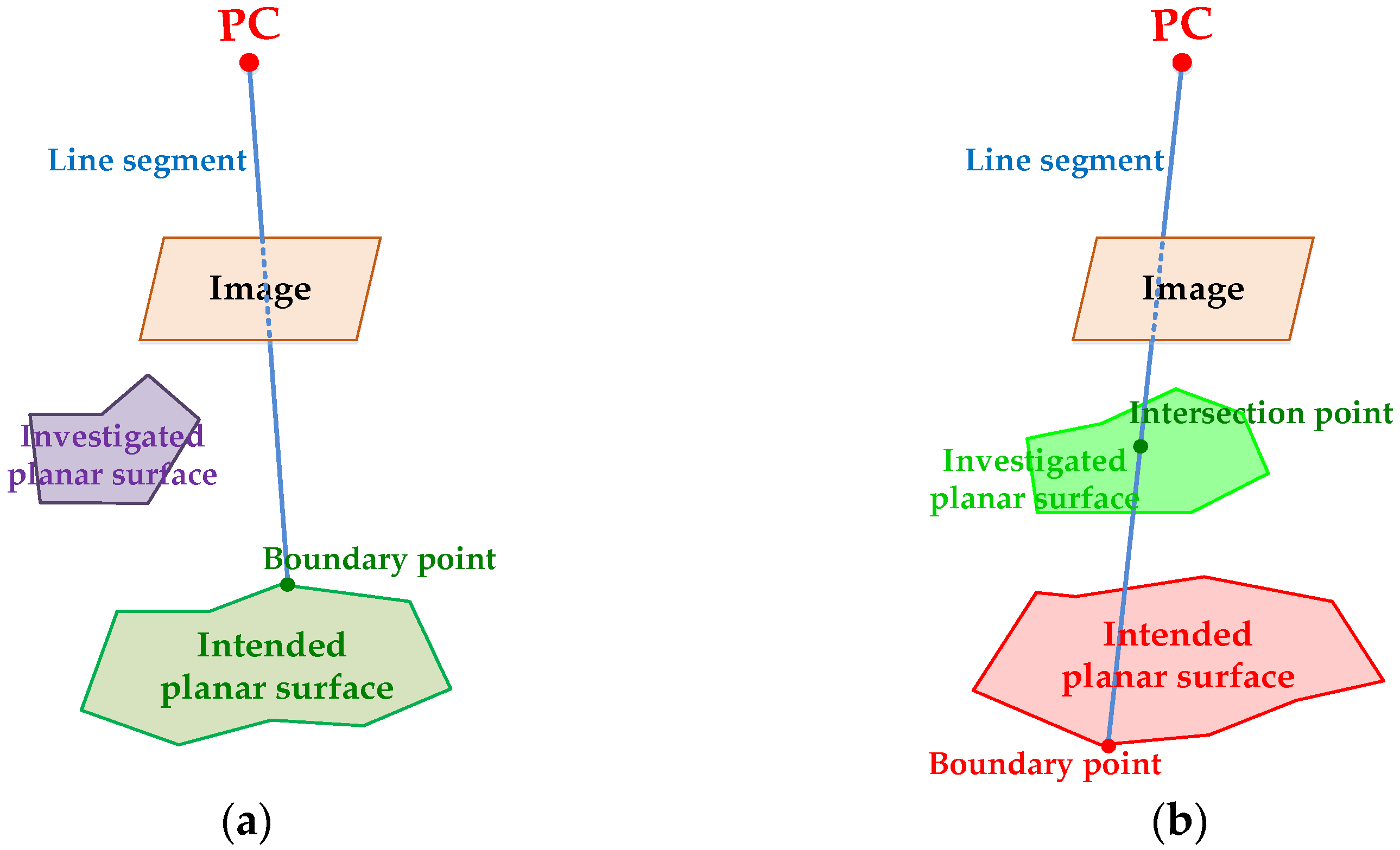
3.2. Occlusion Detection
- The boundary point (as well as its respective planar surface) is occluded by the intersecting planar surface if the latter is closer to the perspective center than the former (green plane in Figure 10).
- The boundary point (as well as its respective planar surface) is occluding the intersecting planar surface if the former is closer to the perspective center than the latter (yellow plane in Figure 10).
3.3. Planar Surface Decomposition
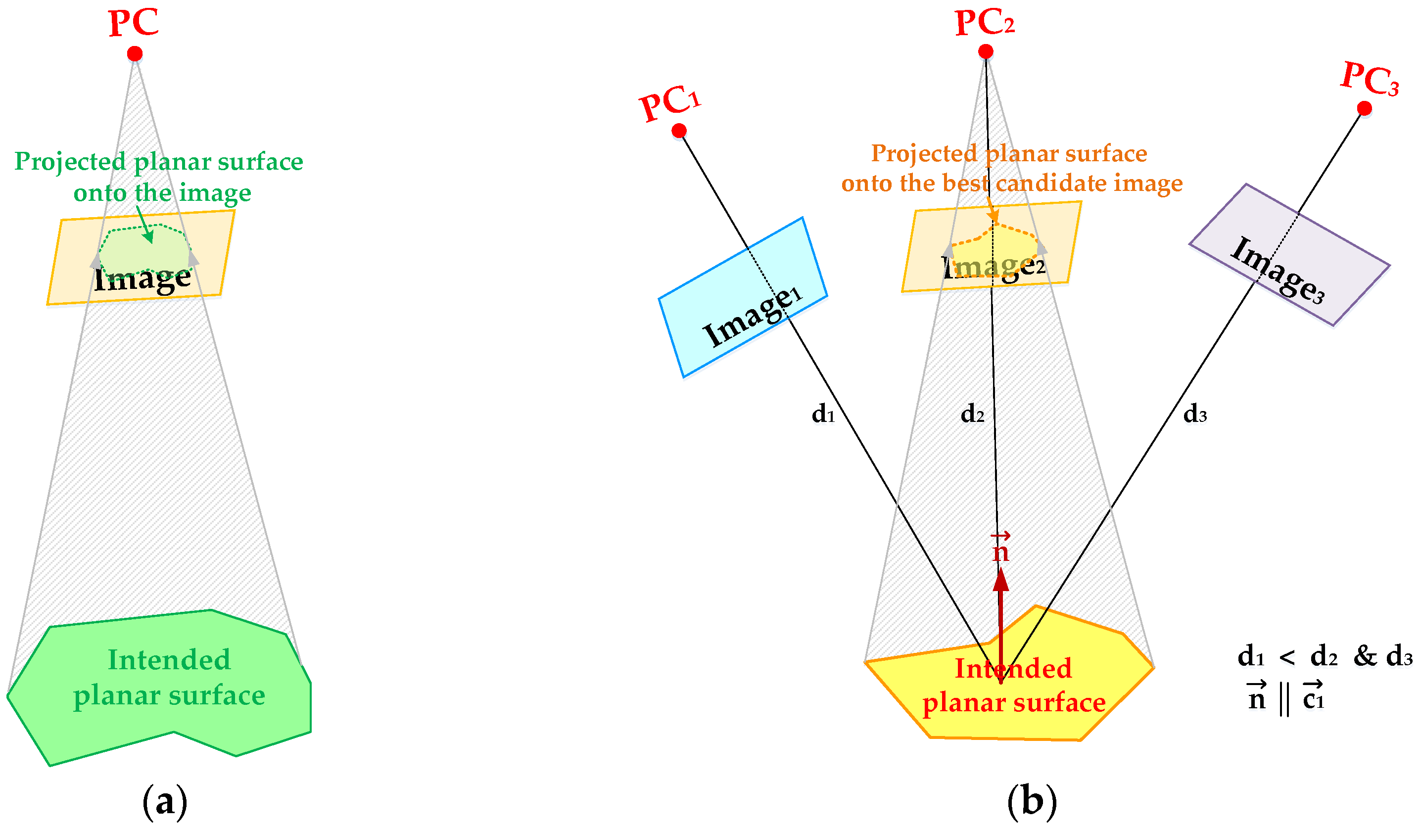
- In the first scenario, the intended planar surface is entirely visible in one or multiple images, which are appropriate for texturing that surface. For a planar surface, which is completely visible in a single image, the rendering procedure will be carried out using that image. However, for the planar surface, which is fully visible in more than one image, the rendering procedure is performed using the image which has the best sampling distance along that surface. This image (either nadir or oblique) is selected as the one which is within an acceptable distance from the surface’s centroid and its optical axis makes the smallest angle with the surface’s normal. In order to identify the best candidate image satisfying the above-mentioned conditions, a cost function is defined as in Equation (1):In this cost function, d is the distance between the perspective center of a candidate image and the centroid of the intended surface, dmax is the maximum allowable distance between the perspective center of an appropriate image and the centroid of the intended surface, is the candidate image’s optical axis, is the normal vector to the intended planar surface, and wd and wang are the weight parameters which determine the contribution of the distance and angle components in the selection of best candidate image. This cost function will be maximized for the image which has the closest distance to the intended surface and the smallest angle between its optical axis and normal to that surface. The respective image is used for rendering the intended surface. Once the most appropriate image for texturing procedure is selected, the boundary points of the intended planar surface are projected onto the chosen image and the part of the image within the projected boundary will be rendered onto the given surface (Figure 13).
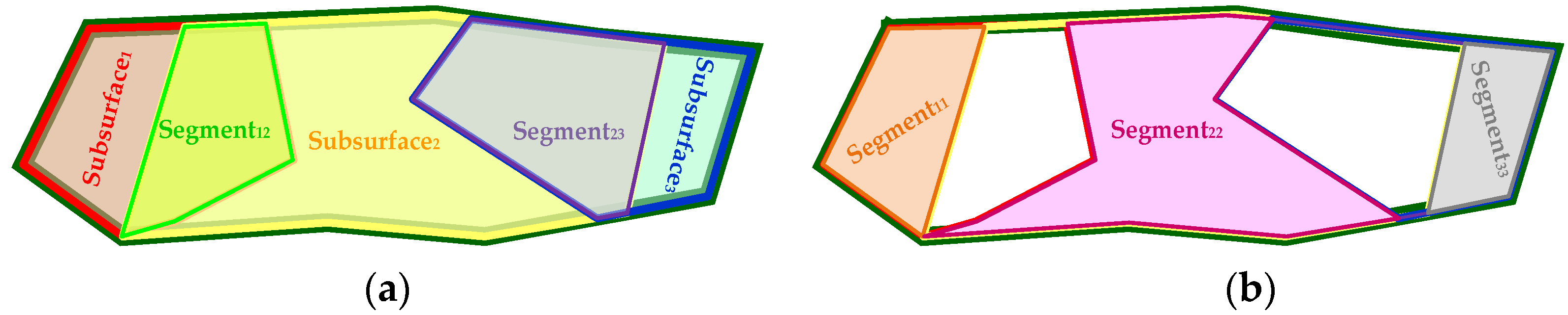
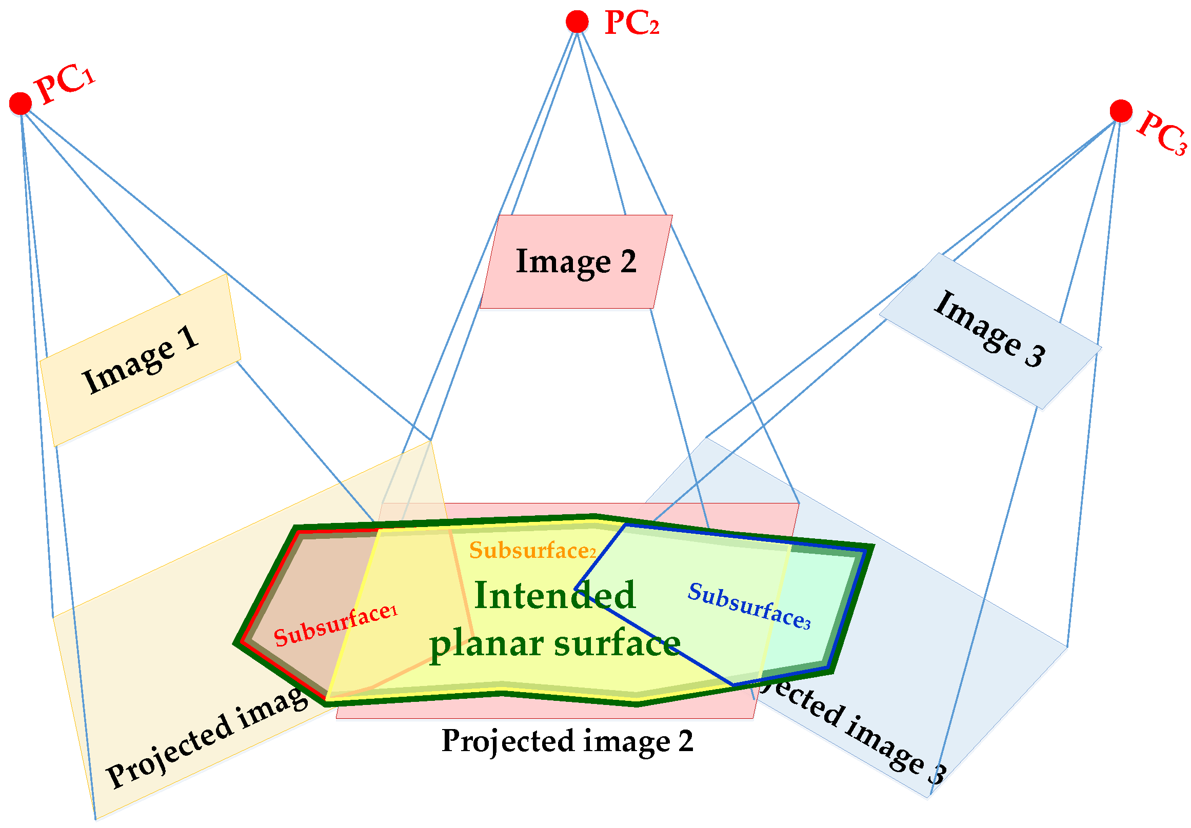
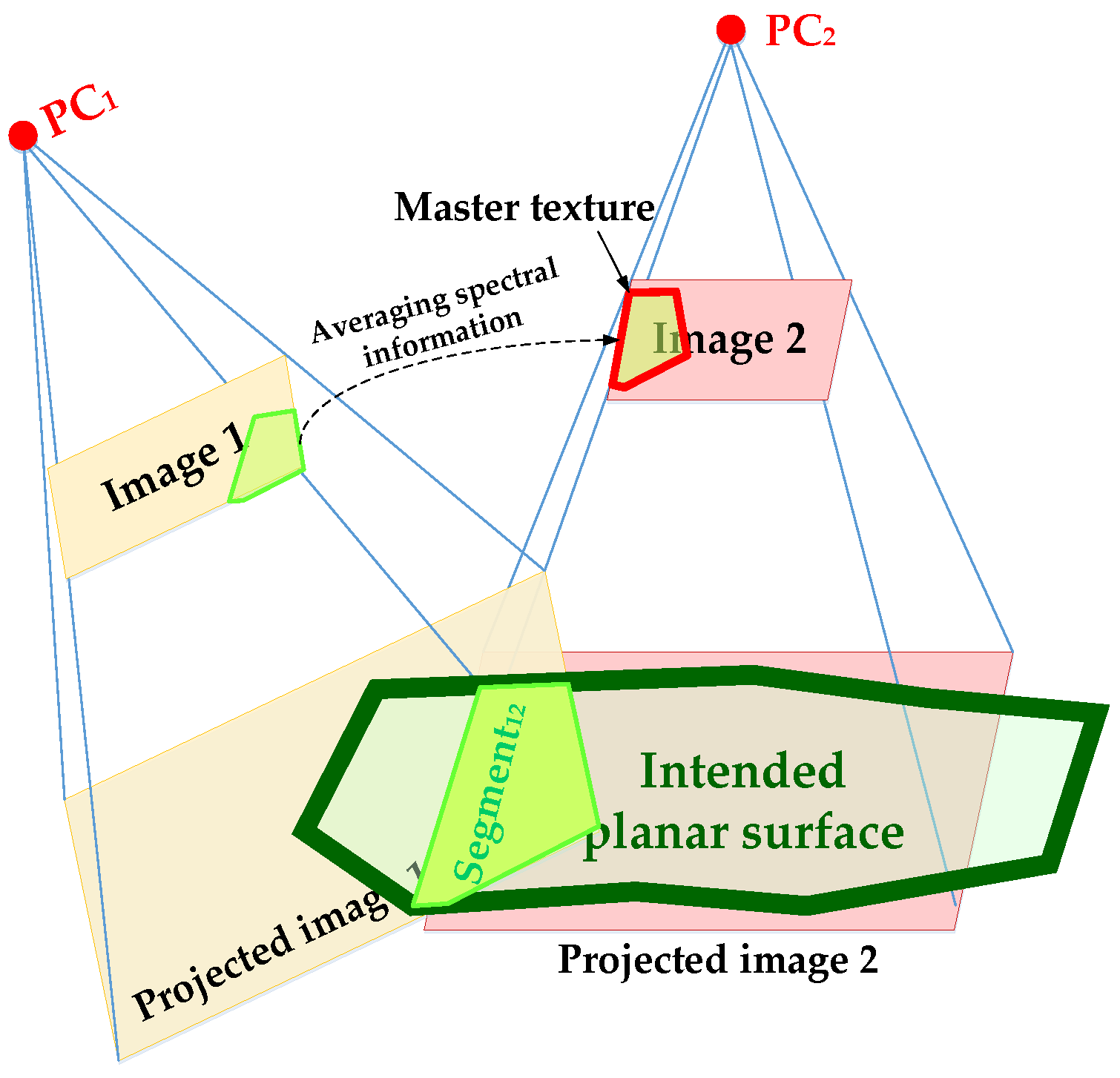
- In the second scenario, the intended surface is partially visible within multiple images. The rendering of such a surface is carried out by decomposing this surface into the segments which are visible in single or multiple appropriate images. In order to delineate these segments, visible/non-occluded parts of the intended surface within individual appropriate images (Figure 14) are first intersected together using the Weiler-Atheron algorithm [56]. The outcome of this polygon intersection procedure will be the segments, which are visible in a single image (e.g., segment11, segment22, and segment33 in Figure 15) or multiple images (e.g., segment12 and segment23 in Figure 15). Figure 15 shows the segments of the intended planar surface that are visible in single or multiple images.For the segments, which are visible in a single image (segment11, segment22, and segment33), the rendering procedure is carried out in the same way as the previous scenario. However, for the segments which are visible in multiple images, the rendering procedure is carried out using all appropriate images including those segments. Accordingly, the boundary points of such a segment are firstly projected onto all the appropriate images enclosing that segment. The projected boundary onto the best candidate image for texturing that segment is selected as the master texture and the spectral information from other enclosing images are incorporated into the identified master texture. In order to accurately integrate the spectral information from multiple images, the correspondence between the conjugate pixels within the projected boundary onto the relevant images is established using a 2D projective transformation (Equation (2)). The coefficients of this 2D projective transformation are derived using the image coordinates of corresponding boundary points projected onto the images through a least-squares adjustment procedure.The assigned color to a pixel within the master texture is ultimately derived by averaging the colors of its conjugate pixels within all images enclosing the intended segment as in Equation (3). This segment will ultimately be textured using the modified master texture. Figure 16 shows the rendering procedure for a segment which is visible in two images (segment12).
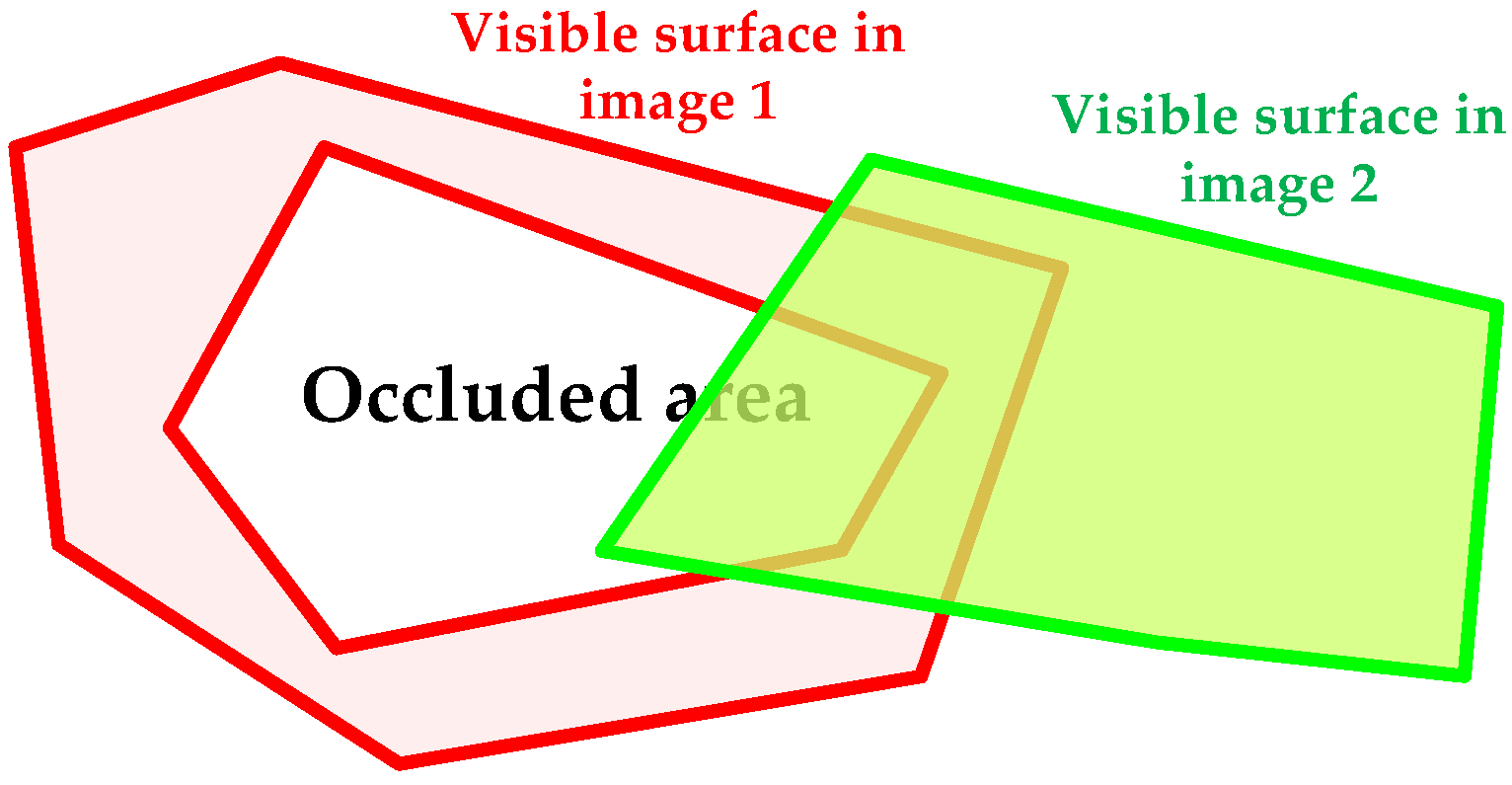
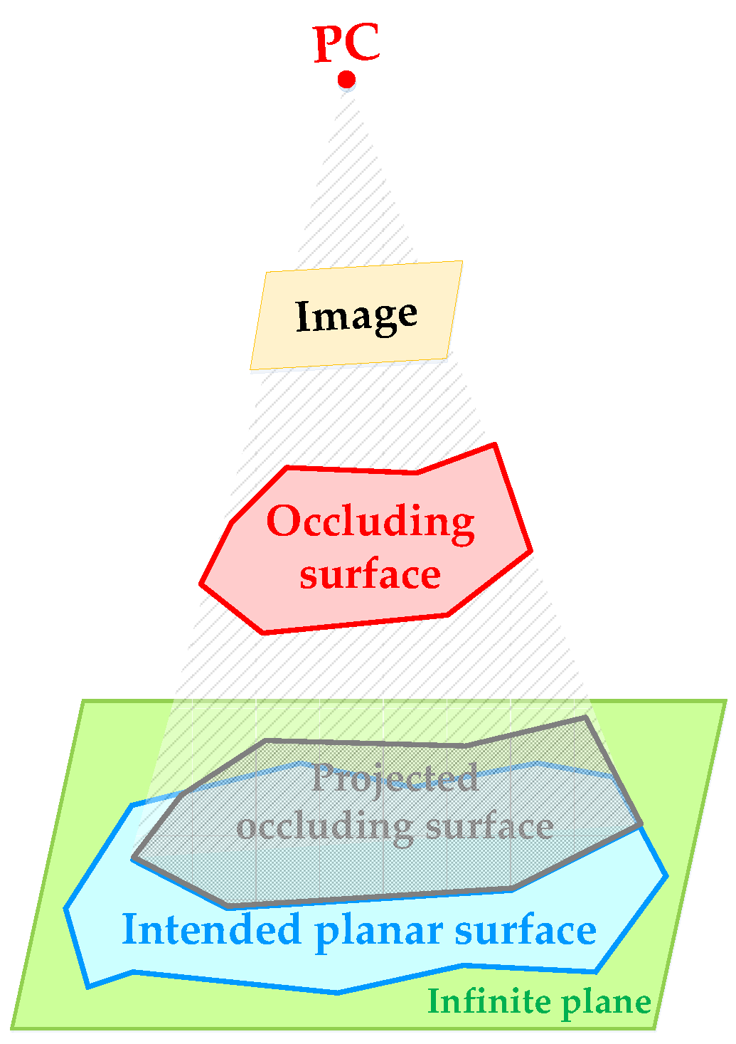
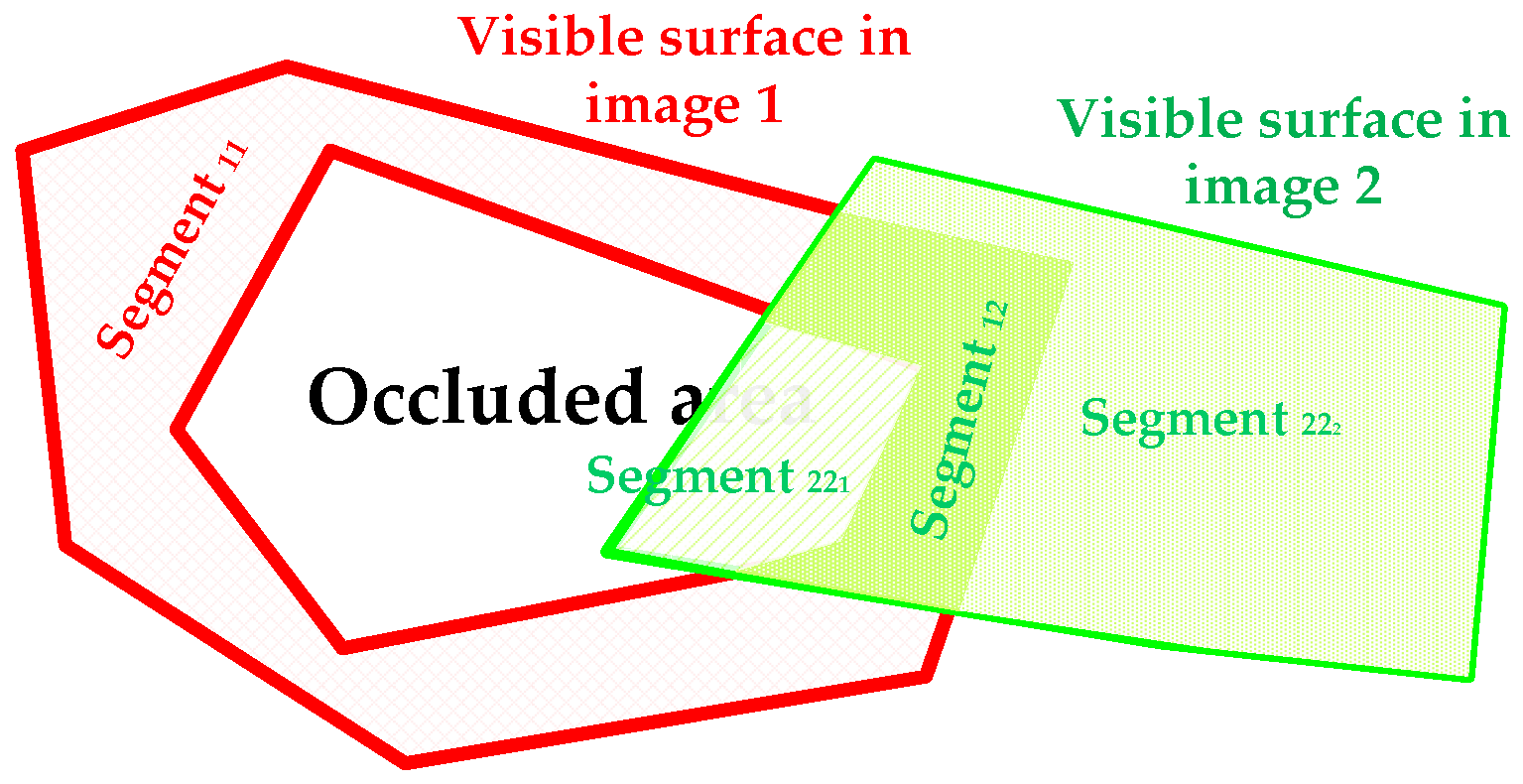
- In the third scenario, which occurs in special cases, a planar surface is partially occluded by other planar surface/surfaces in the field of view of the best candidate image for texturing that surface. In such a case, the rendering procedure for the intended surface is performed after excluding the occluded area from that surface. However, some parts of the occluded/excluded area might be visible in other images. Hence, the intersection between the visible surfaces within multiple images is carried out to determine the parts of the occluded area within a surface that can be textured using the other images. Figure 17 shows the intersection between two surfaces which are partially visible in two images, where one of them has an occluded area inside. Figure 18 shows the segments of these surfaces which are visible in single or multiple images. As seen in Figure 18, a part of the occluded area within visible surface in image 1 is covered by the visible surface in image 2 (segment222). Therefore, segment11 will be projected onto and textured using image 1, segment221 and segment222 will be projected onto and textured using image 2, and segment12 will be projected onto and textured using both images.
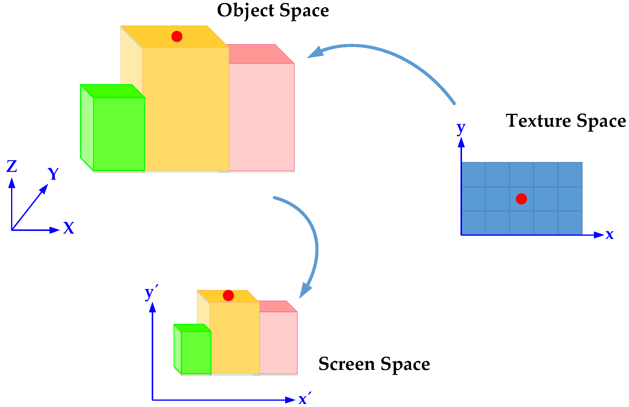
3.4. Rendering and Visualization
- Texture space (2D image space),
- 3D object space, and
- 2D screen space.
3.4.1. Tessellation
- No other vertex lies within the interior of any of the circumcircles of the triangles constructed by three nearby vertices in the planar surface (Figure 21).
- The minimum interior angle is maximized, and the maximum is minimized. Therefore, triangles are generated as equiangular as possible and long and thin triangles are avoided.
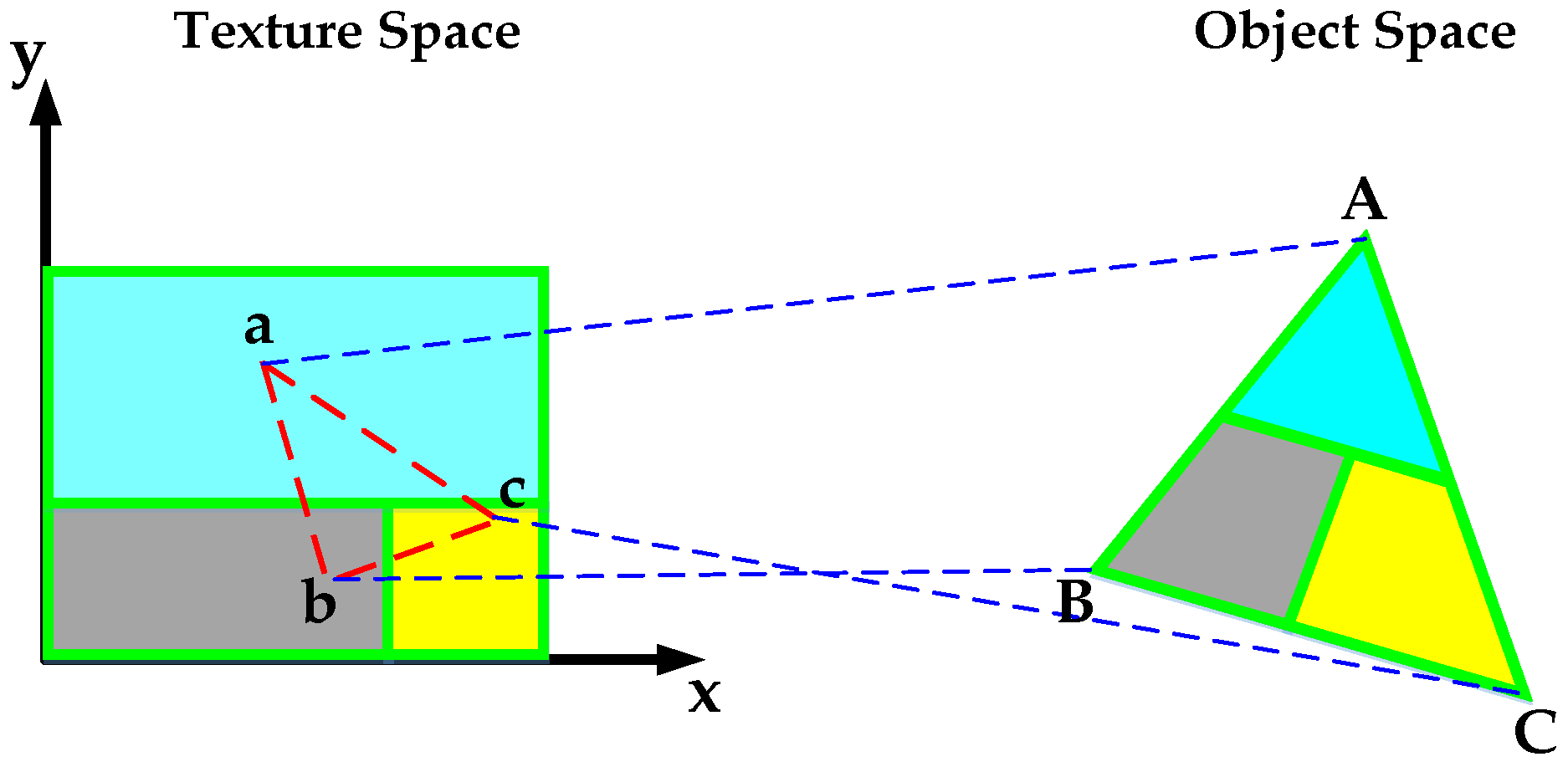
3.4.2. Texture Mapping
- Specification of the texture,
- Assignment of texture coordinates to the triangulated polygon vertices,
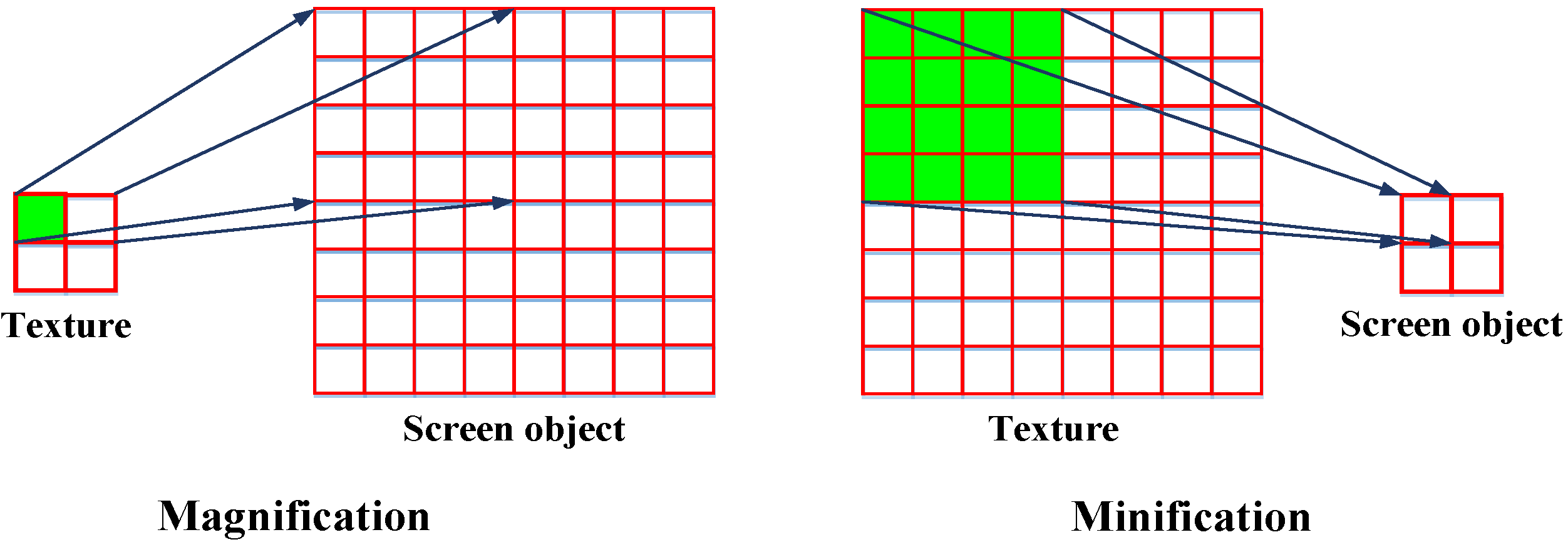
- Specification of filtering method, and
- Drawing the surfaces on the screen using geometric coordinates and texture images.
4. Experimental Results
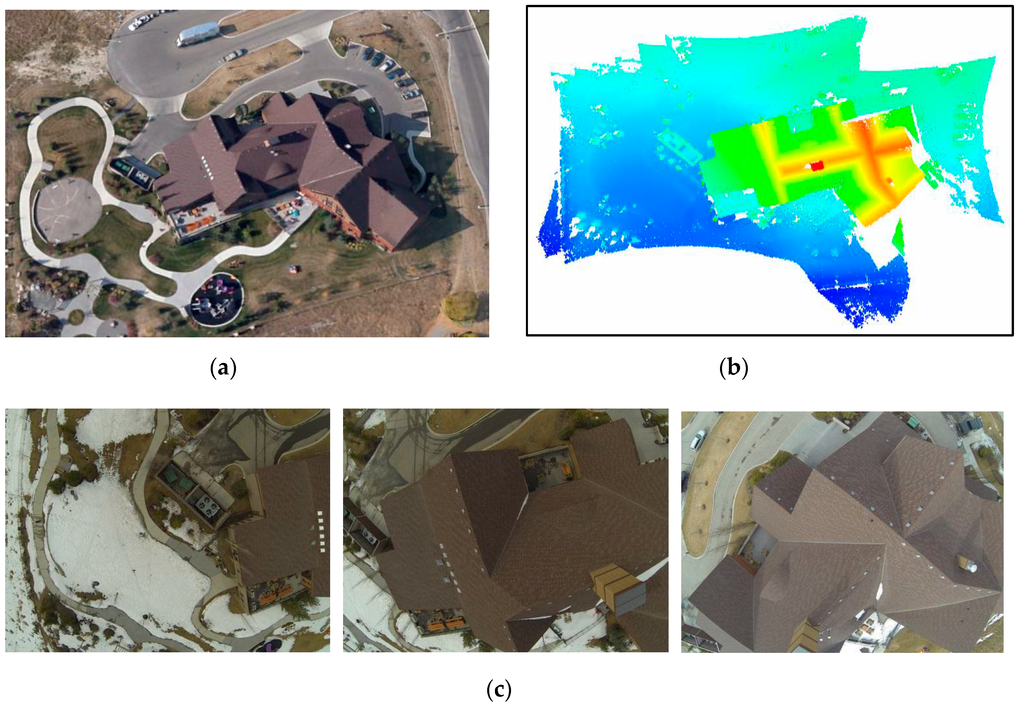
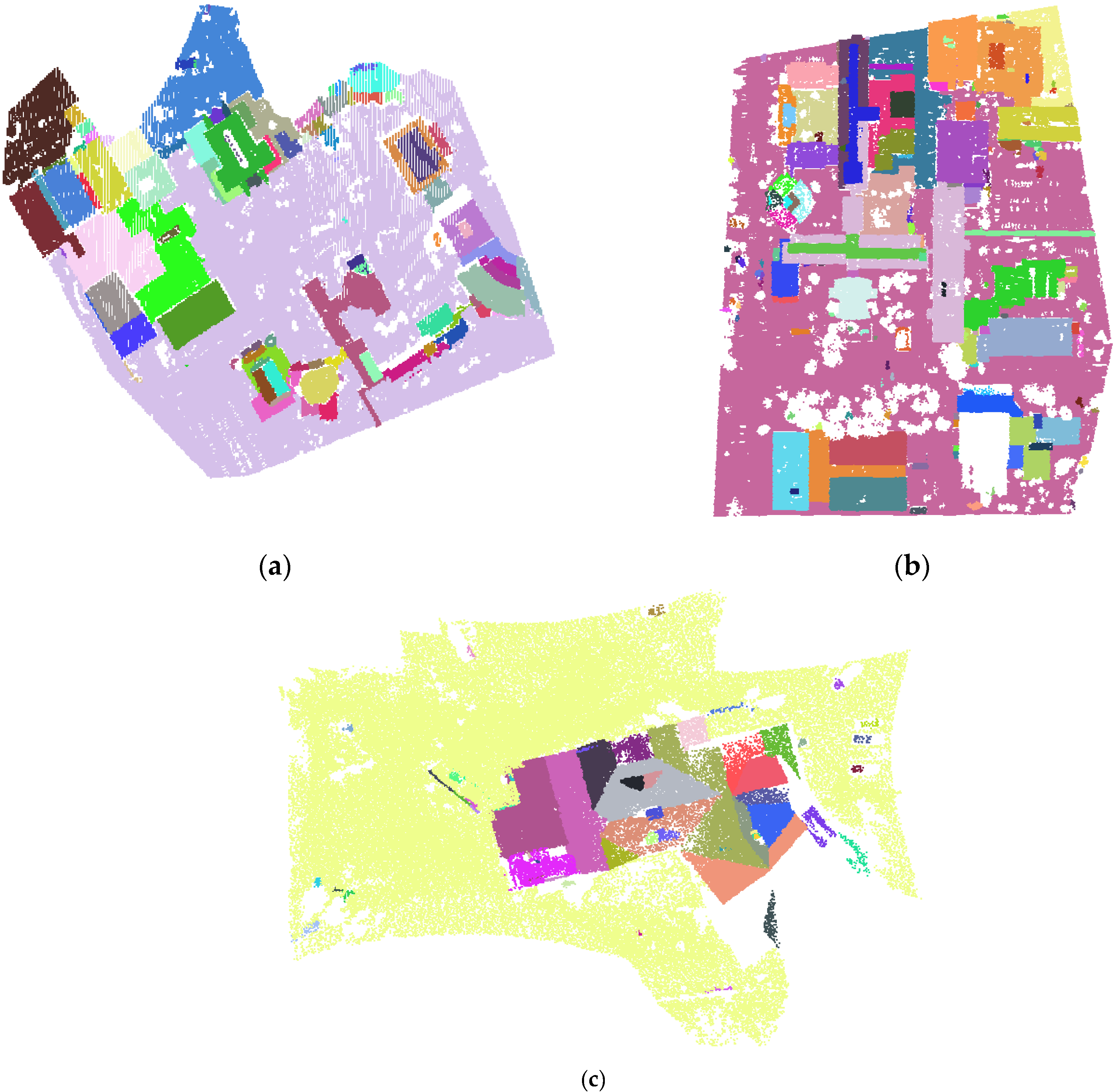
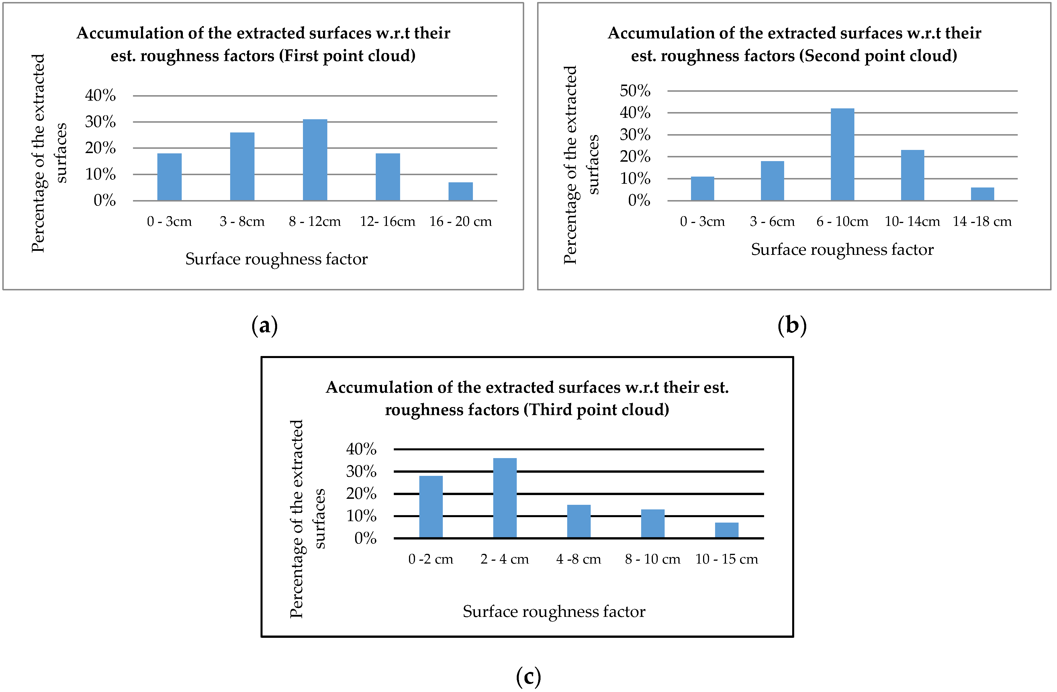
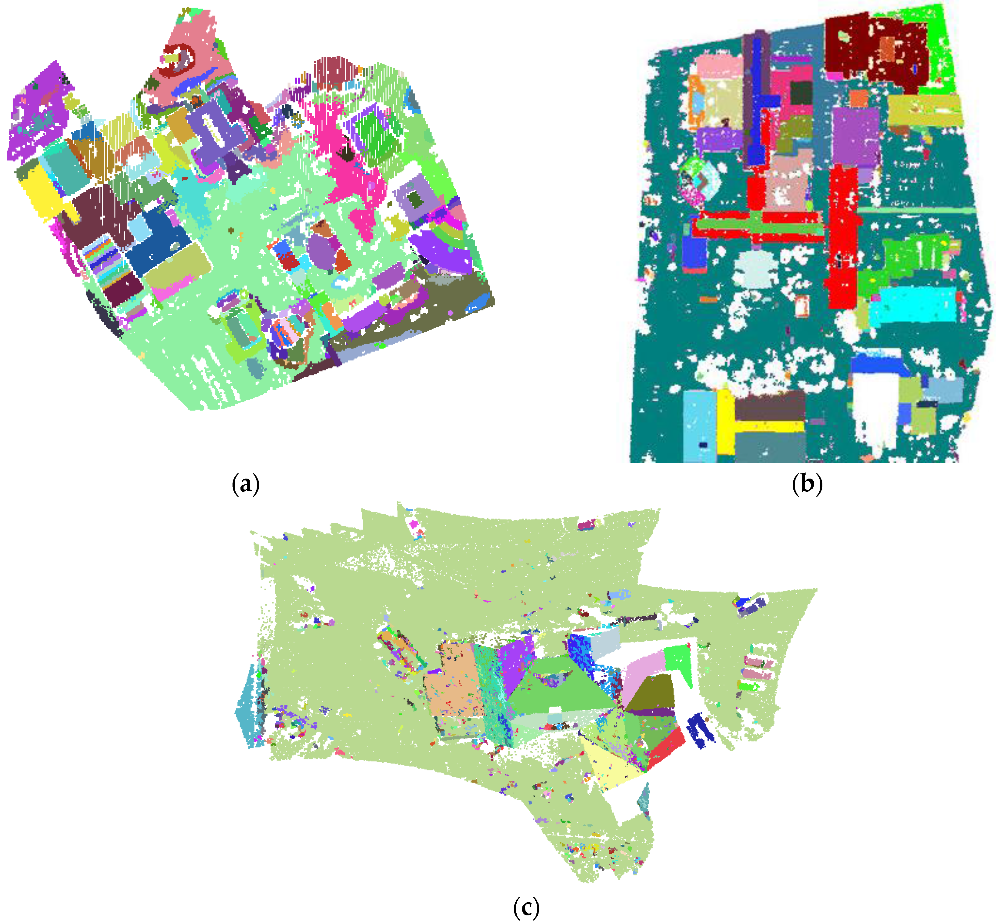
4.1. Quality Control of the Extracted Planar Surfaces from Laser Scanning Data
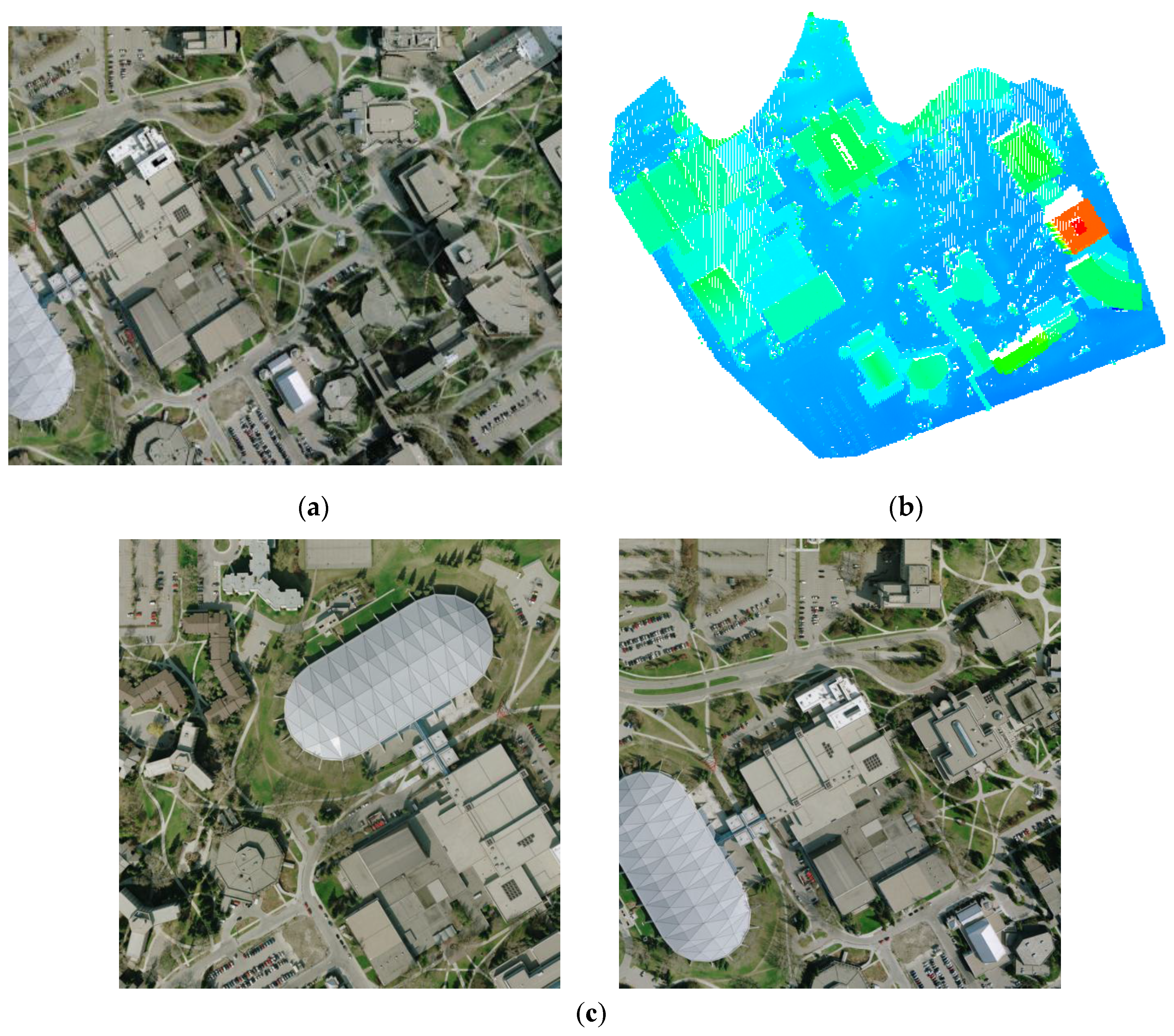
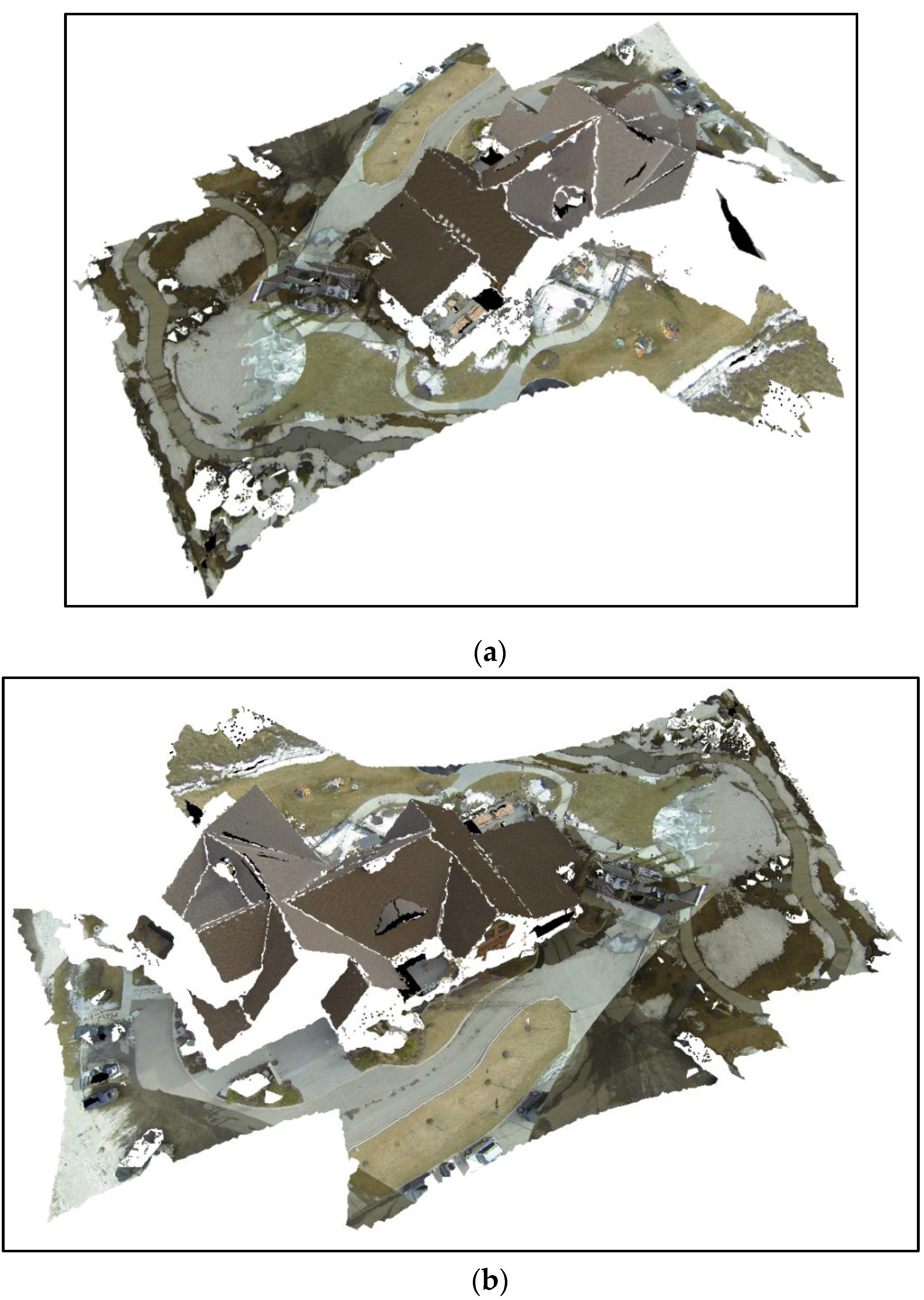
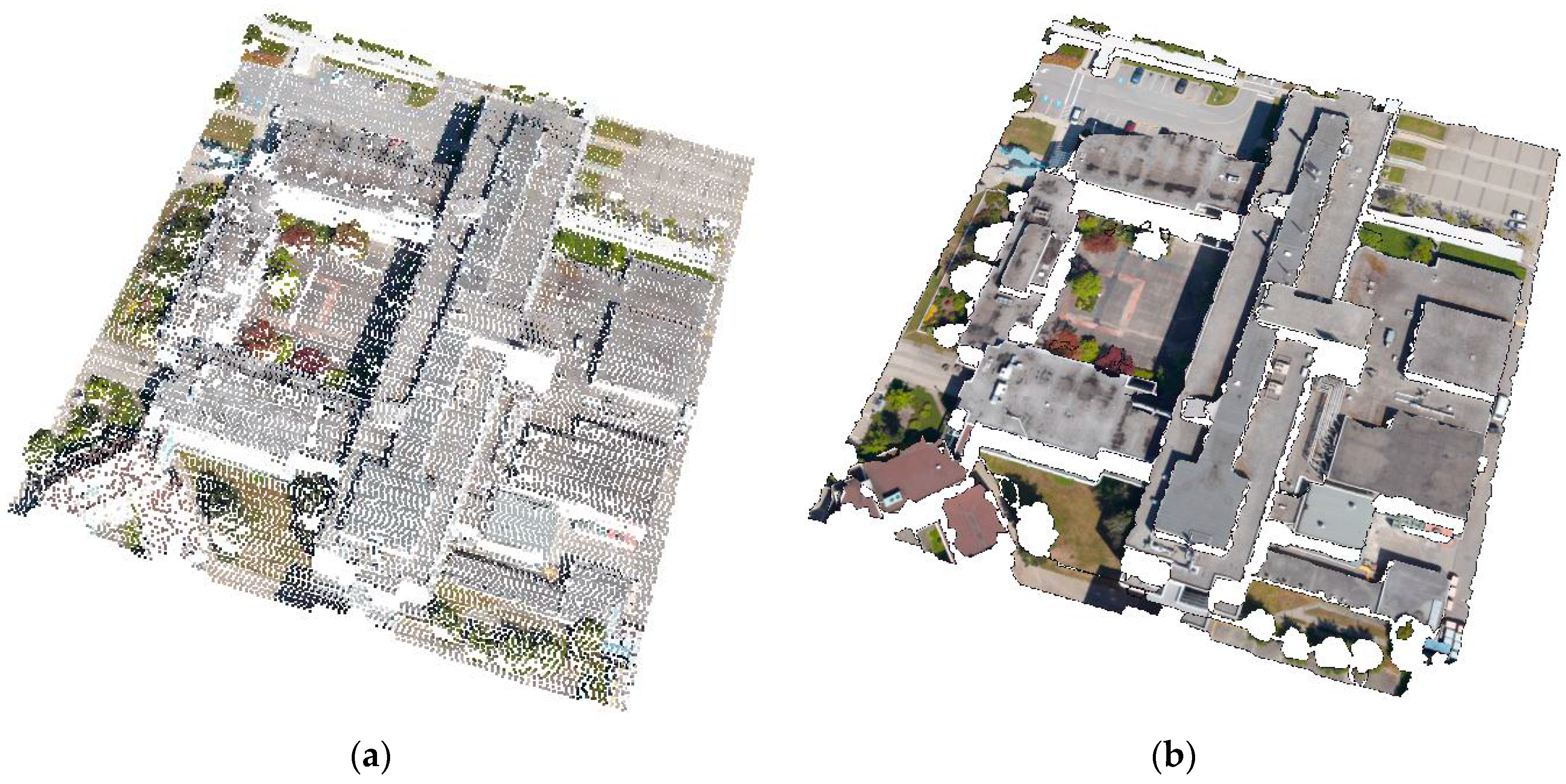
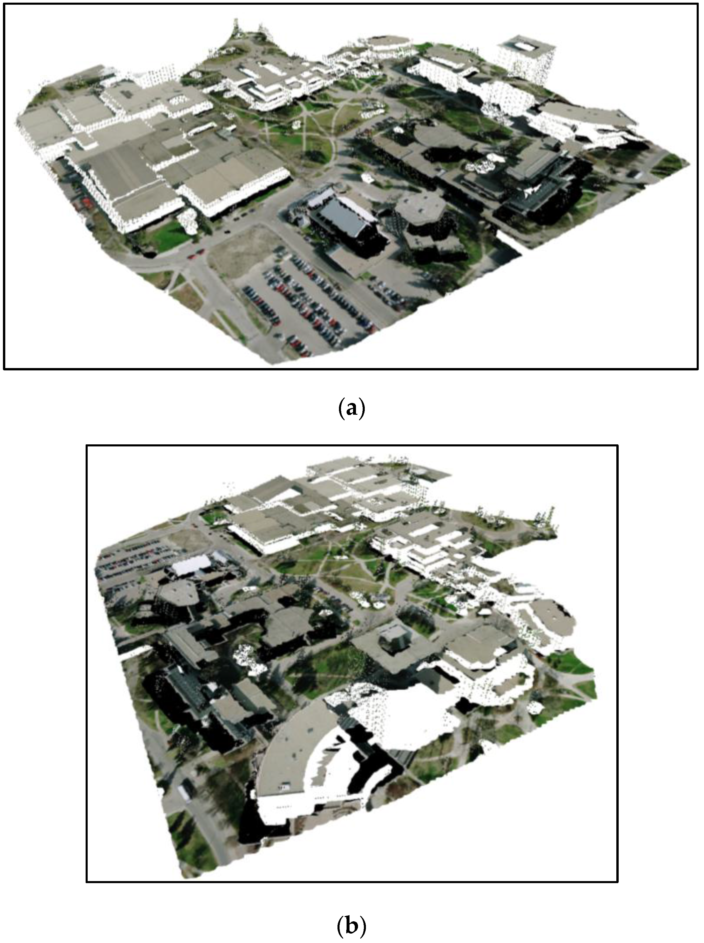
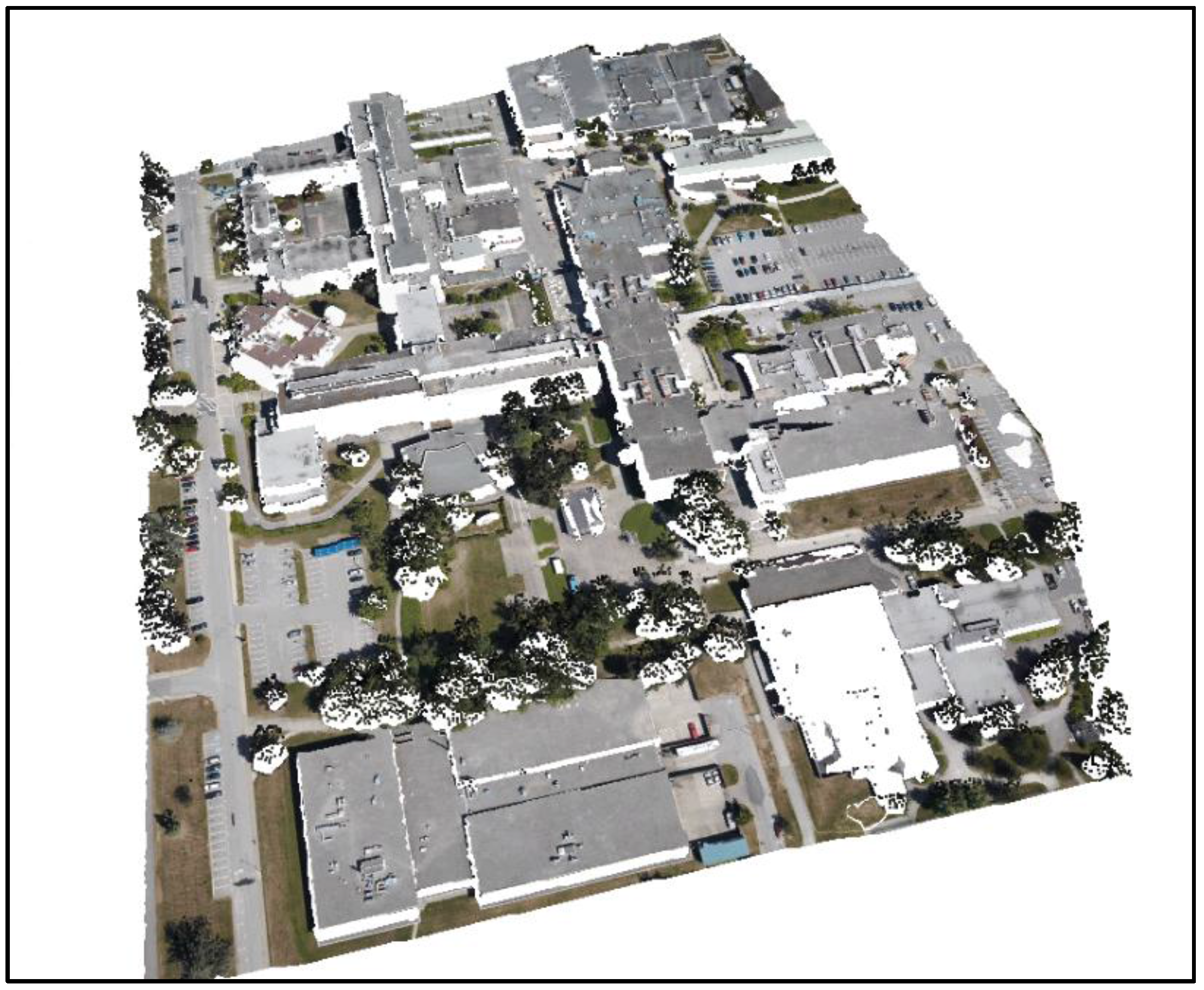
4.2. Evaluation of Realistic 3D Reconstruction of the Extracted Planar Surfaces Using Acquired Imagery
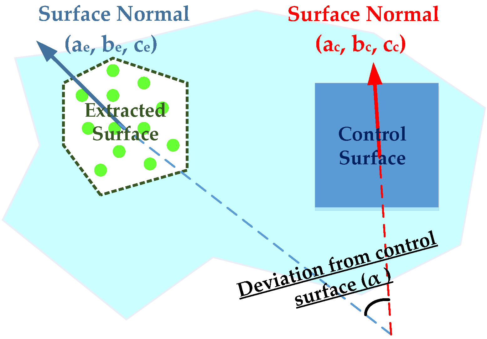
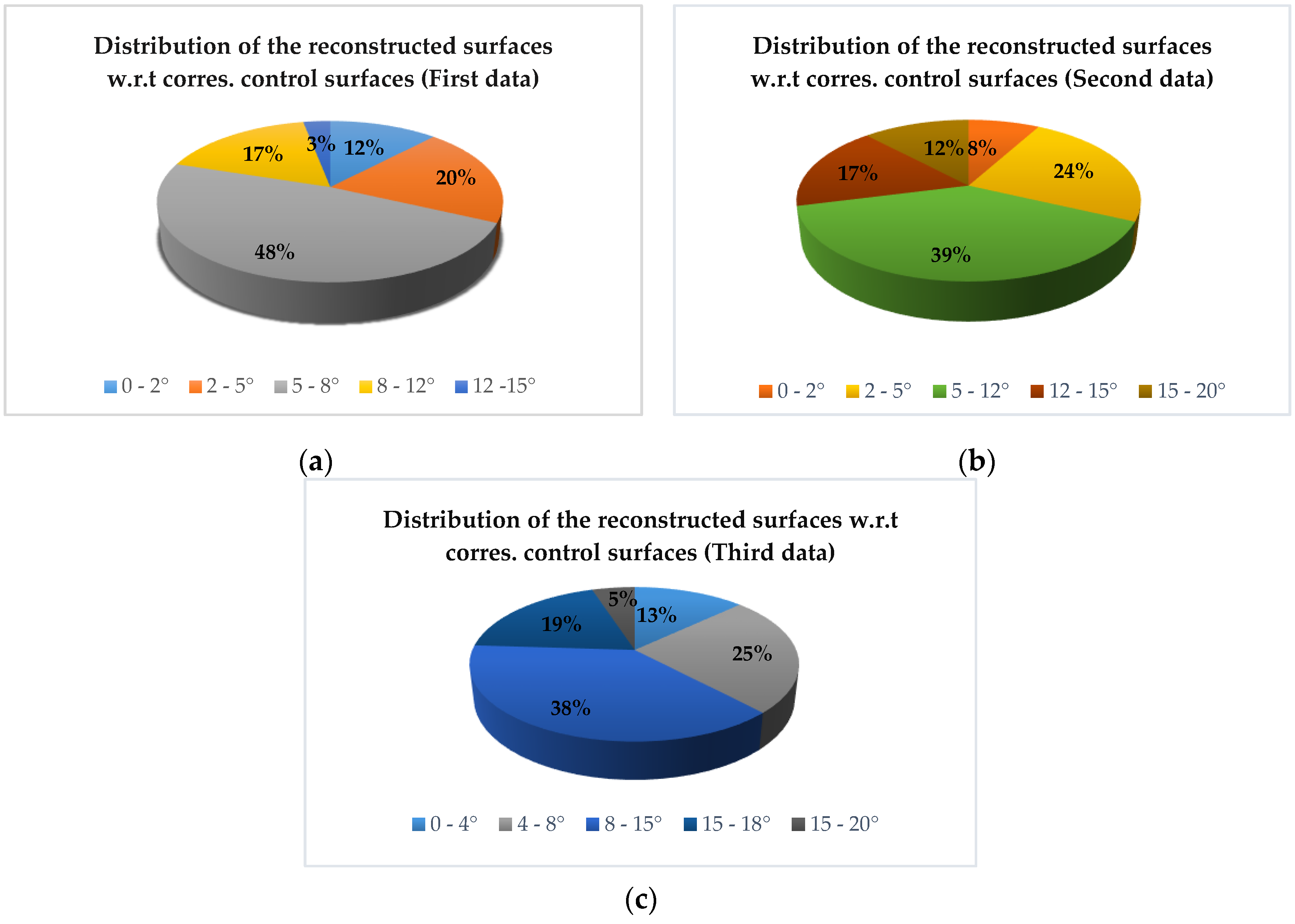
4.3. Quality Control of 3D Surface Reconstruction Outcome
4.4. Evaluation of the Computational Efficiency of the Proposed 3D Scene Reconstruction Technique
5. Conclusions and Recommendations for Future Research Work
- Implementation a surface-based 3D surface reconstruction procedure as opposed to previously-developed point-based techniques,
- Expansion of the occlusion/visibility analysis approaches to handle surface-based texturing procedure,
- Rendering the extracted surfaces using the images where they are fully or partially visible, and,
- Enhancement of the interpretability of the segmented planar surfaces.
Acknowledgments
Author Contributions
Conflicts of Interest
References
- Poullis, C.; You, S. 3D reconstruction of urban areas. In Proceedings of the Visualization and Transmission 2011 International Conference on 3D Imaging, Modeling, Processing, Visualization and Transmission, Hangzhou, China, 16–19 May 2011; pp. 33–40.
- Campos, R.; Garcia, R.; Alliez, P.; Yvinec, M. A surface reconstruction method for in-detail underwater 3D optical mapping. Int. J. Rob. Res. 2015, 34, 64–89. [Google Scholar] [CrossRef]
- Kwak, E.; Detchev, I.; Habib, A.; El-badry, M.; Hughes, C. Precise photogrammetric reconstruction using model-based image fitting for 3D beam deformation monitoring. J. Surv. Eng. 2013, 139, 143–155. [Google Scholar] [CrossRef]
- Remondino, F. Heritage recording and 3D Modeling with Photogrammetry and 3D Scanning. Remote Sens. 2011, 3, 1104–1138. [Google Scholar] [CrossRef] [Green Version]
- Zou, Y.; Chen, W.; Wu, X.; Liu, Z. Indoor localization and 3D scene reconstruction for mobile robots using the Microsoft Kinect sensor. In Proceedings of the IEEE 10th International Conference on Industrial Informatics, Beijing, China, 25–27 July 2012; pp. 1182–1187.
- Kemec, S.; Sebnem Duzgun, H.; Zlatanova, S. A conceptual framework for 3D visualization to support urban disaster management. In Proceedings of the Joint Symposium of ICA WG on CEWaCM and JBGIS Gi4DM, Praugue, Czech, 19–22 January 2009; pp. 268–278.
- Arefi, H. From LIDAR Point Clouds to 3D Building Models. Thesis, University of Tehran, Tehran, Iran, 2009. [Google Scholar]
- Vosselman, G.; Maas, H.-G. Airborne and Terrestrial Laser Scanning; Whittles Publishing: Dunbeath, Scotland, 2010. [Google Scholar]
- Lari, Z.; El-Sheimy, N. System considerations and challenges in 3d mapping and modelling using low-cost UAV images. ISPRS Int. Arch. Photogramm. Remote Sens. Spat. Inf. Sci. 2015, XL-3/W3, 343–348. [Google Scholar] [CrossRef]
- Nex, F.; Remondino, F. UAV for 3D mapping applications: A review. Appl. Geomat. 2014, 6, 1–15. [Google Scholar] [CrossRef]
- Lamond, B.; Watson, G. Hybrid rendering - a new integration of photogrammetry and laser scanning for image based rendering. In Proceedings of the Theory and Practice of Computer Graphics, Bournemouth, UK, 8–10 June 2004; pp. 179–186.
- Alshawabkeh, Y.; Haala, N. Automatic multi-image photo-texturing of complex 3D scenes. In Proceedings of the CIPA 2005 XX International Symposium, Torino, Italy, 26 September–1 October 2005.
- El-Omari, S.; Moselhi, O. Integrating 3D laser scanning and photogrammetry for progress measurement of construction work. Autom. Constr. 2008, 18, 1–9. [Google Scholar] [CrossRef]
- Koch, M.; Kaehler, M. Combining 3D laser-scanning and close-range Photogrammetry: An approach to exploit the strength of both methods. In Proceedings of the 37th International Conference on Computer Applications to Archaeology, Williamsburg, VA, USA, 22–26 March 2009; pp. 1–7.
- Kim, C.; Habib, A. Object-based integration of photogrammetric and LiDAR data for automated generation of complex polyhedral building models. Sensors 2009, 9, 5679–5701. [Google Scholar] [CrossRef] [PubMed]
- Nex, F.; Remondino, F.; Rinaudo, F. Integration of range and image data for building reconstruction. In Proceedings of the Videometrics, Range Imaging, and Applications XI 2011, Munich, Germany, 23 May 2011; Volume 8085, pp. 80850A:1–80850A:14.
- Lerma, J.L.; Navarro, S.; Cabrelles, M.; Seguí, A.E.; Haddad, N.; Akasheh, T. Integration of Laser Scanning and Imagery for Photorealistic 3D Architectural Documentation. In Laser Scanning, Theory and Applications; Wang, C.-C., Ed.; InTech: Rijeka, Croatia, 2011; pp. 413–430. [Google Scholar]
- Moussa, W. Integration of Digital Photogrammetry and Terrestrial Laser Scanning for Cultural Heritage Data Recording; University of Stuttgart: Stuttgart, Germany, 2014. [Google Scholar]
- Kwak, E.; Habib, A. Automatic representation and reconstruction of DBM from LiDAR data using Recursive Minimum Bounding Rectangle. ISPRS J. Photogramm. Remote Sens. 2014, 93, 171–191. [Google Scholar] [CrossRef]
- Lichtenauer, J.F.; Sirmacek, B. A semi-automatic procedure for texturing of laser scanning point cloouds with Google streetview images. ISPRS Int. Arch. Photogramm. Remote Sens. Spat. Inf. Sci. 2015, XL-3-W3, 109–114. [Google Scholar] [CrossRef]
- Habib, A.; Ghanma, M.; Mitishita, E.A. Co-registration of photogrammetric and LiDAR data: Methodology and case study. Braz. J. Cartogr. 2004, 56, 1–13. [Google Scholar]
- Chen, L.; Teo, T.; Shao, Y.; Lai, Y.; Rau, J. Fusion of LiDAR data and optical imagery for building modeling. Int. Arch. Photogramm. Remote Sens. Spat. Inf. Sci. 2004, 35 (Pt. B4), 732–737. [Google Scholar]
- Habib, A.; Schenk, T. New approach for matching surfaces from laser scanners and optical sensors. Int. Arch. Photogramm. Remote Sens. Spat. Inf. Sci. 1999, 32, 55–61. [Google Scholar]
- Vosselman, G.; Gorte, B.G.H.; Sithole, G.; Rabbani, T. Recognising structure in laser scanner point clouds. Int. Arch. Photogramm. Remote Sens. Spat. Inf. Sci. 2004, 8-W2, 33–38. [Google Scholar]
- Guelch, E. Advanced matching techniques for high precision surface and terrain models. In Proceedings of the Photogrammetric Week 2009, Heidelberg, Germany, 7–11 September 2009; pp. 303–315.
- Kazhdan, M.; Bolitho, M.; Hoppe, H. Poisson surface reconstruction. In Proceedings of the Symposium on Geometry Processing 2006, Sardinia, Italy, 26–28 June 2006; pp. 61–70.
- Kraus, K. Photogrammetry, Volume 1, Fundamentals and Standard Processes; Dummler Verlag: Bonn, Germany, 1993. [Google Scholar]
- Novak, K. Rectification of digital imagery. Photogramm. Eng. Remote Sens. 1992, 58, 339–344. [Google Scholar]
- Habib, A.; Kim, E.M.; Kim, C. New methodologies for true orthophoto generation. Photogramm. Eng. Remote Sens. 2007, 73, 25–36. [Google Scholar] [CrossRef]
- El-Hakim, S.F.; Remondino, F.; Voltolini, F. Integrating Techniques for Detail and Photo-Realistic 3D Modelling of Castles. GIM Int. 2003, 22, 21–25. [Google Scholar]
- Wang, L.; Kang, S.B.; Szeliski, R.; Sham, H.Y. Optimal texture map generation using multiple views. In Proceedings of the Computer Vision and Pattern Recognition, Kauai, HI, USA, 8–14 December 2001; pp. 347–354.
- Bannai, N.; Fisher, R.B.; Agathos, A. Multiple color texture map fusion for 3D models. Pattern Recognit. Lett. 2007, 28, 748–758. [Google Scholar] [CrossRef]
- Xu, L.; Li, E.; Li, J.; Chen, Y.; Zhang, Y. A general texture mapping framework for image-based 3D modeling. In Proceedings of the 17th IEEE International Conference on Image Processing (ICIP), Hong Kong, China, 26–29 September 2010; pp. 2713–2716.
- Zhu, L.; Hyyppä, J.; Kukko, A.; Kaartinen, H.; Chen, R. Photorealistic building reconstruction from mobile laser scanning data. Remote Sens. 2011, 3, 1406–1426. [Google Scholar] [CrossRef]
- Chen, Z.; Zhou, J.; Chen, Y.; Wang, G. 3D texture mapping in multi-view reconstruction. In Advances in Visual Computing; Lecture Notes in Computer Science; Springer: Berlin, Germany, 2012; pp. 359–371. [Google Scholar]
- Ahmar, F.; Jansa, J.; Ries, C. The generation of true orthophotos using a 3D building model in conjunction with a conventional DTM. Int. Arch. Photogramm. Remote Sens. Spat. Inf. Sci. 1998, 32(Pt. 4), 16–22. [Google Scholar]
- Watkins, G.S. A Real-Time Visible Surface Algorithm; Computer Science, University of Utah: Salt Lake City, UT, USA, 1970. [Google Scholar]
- Laine, S.; Karras, T. Two methods for fast ray-cast ambient occlusion. In Proceedings of the Eurographics Symposium on Rendering, Saarbrücken, Germany, 28–30 June 2010. [CrossRef]
- Heckbert, P.; Garland, M. Multiresolution modeling for fast rendering. In Proceedings of Graphics Interface ’94, Banff, AB, Canada, 18–20 May 1994; pp. 43–50.
- Mikhail, E.M.; Bethel, J.; McGline, C. Introduction to Modern Photogrammetry; Wiley and Sons: Hoboken, NJ, USA, 2001. [Google Scholar]
- Oliveira, H.C.; Galo, M. Occlusion detection by height gradient for true orthophoto generation using LiDAR data. ISPRS Int. Arch. Photogramm. Remote Sens. Spat. Inf. Sci. 2013, XL-1-W1, 275–280. [Google Scholar] [CrossRef]
- Kuzmin, Y.P.; Korytnik, S.A.; Long, O. Polygon-based true orthophoto generation. Int. Arch. Photogramm. Remote Sens. Spat. Inf. Sci. 2004, XXXV, 529–531. [Google Scholar]
- Chen, L.-C.; Teo, T.-A.; Wen, J.-Y.; Rau, J.-Y. Occlusion-compensated true orthorectification for high-resolution satellite images. Photogramm. Rec. 2007, 22, 39–52. [Google Scholar] [CrossRef]
- Tran, A.T.; Harada, K. Depth-aided tracking multiple objects under occlusion. J. Signal Inf. Process. 2013, 4, 299–307. [Google Scholar] [CrossRef]
- Kovalčík, V.; Sochor, J. Fast rendering of complex dynamic scenes. 2006, 81–87. [Google Scholar]
- Lari, Z.; Habib, A. An adaptive approach for the segmentation and extraction of planar and linear/cylindrical features from laser scanning data. ISPRS J. Photogramm. Remote Sens. 2014, 93, 192–212. [Google Scholar] [CrossRef]
- Bang, K.I. Alternative methodologies for LiDAR system calibration. Ph.D. Dissertation, University of Calgary, Calgary, AB, Canada, 2010. [Google Scholar]
- Habib, A.; Bang, K.I.; Kersting, A.P.; Lee, D.-C. Error budget of LiDAR systems and quality control of the derived data. Photogramm. Eng. Remote Sens. 2009, 75, 1093–1108. [Google Scholar] [CrossRef]
- Habib, A.F.; Kersting, A.P.; Bang, K.-I.; Zhai, R.; Al-Durgham, M. A strip adjustment procedure to mitigate the impact of inaccurate mounting parameters in parallel lidar strips. Photogramm. Rec. 2009, 24, 171–195. [Google Scholar] [CrossRef]
- Habib, A.; Bang, K.-I.; Kersting, A.P.; Chow, J. Alternative methodologies for LiDAR system calibration. Remote Sens. 2010, 2, 874–907. [Google Scholar] [CrossRef]
- Pauly, M.; Gross, M.; Kobbelt, L.P. Efficient simplification of point-sampled surfaces. In Proceedings of the Conference on Visualization (VIS); IEEE Computer Society: Washington, DC, USA, 2002; pp. 163–170. [Google Scholar]
- Filin, S.; Pfeifer, N. Neighborhood systems for airborne laser data. Photogramm. Eng. Remote Sens. 2005, 71, 743–755. [Google Scholar] [CrossRef]
- Lari, Z.; Habib, A. New approaches for estimating the local point density and its impact on LiDAR data segmentation. Photogramm. Eng. Remote Sens. 2013, 79, 195–207. [Google Scholar] [CrossRef]
- Samet, H. An overview of quadtrees, octrees, and related hierarchical data structures. In Theoretical Foundations of Computer Graphics and CAD; Earnshaw, D.R.A., Ed.; NATO ASI Series; Springer: Berlin, Germany, 1988; pp. 51–68. [Google Scholar]
- Lari, Z.; Habib, A. A new approach for segmentation-based texturing of laser scanning data. ISPRS - Int. Arch. Photogramm. Remote Sens. Spat. Inf. Sci. 2015, XL-5/W4, 115–121. [Google Scholar] [CrossRef]
- Weiler, K.; Atherton, P. Hidden surface removal using polygon area sorting. In Proceedings of the 4th Annual Conference on Computer Graphics and Interactive Techniques, San Jose, CA, USA, 20–22 July 1977; ACM: New York, NY, USA, 1977; pp. 214–222. [Google Scholar]
- Lari, Z. Adaptive Processing of Laser Scanning Data and Texturing of the Segmentation Outcome. Ph.D. Thesis, University of Calgary, Calgary, AB, USA, 2014. [Google Scholar]
- Shreiner, D. OpenGL Programming Guide: The Official Guide to Learning OpenGL, Versions 3.0 and 3.1, 7th ed.; Addison-Wesley Professional: Indianapolis, IN, USA, 2009. [Google Scholar]
- Bowyer, A. Computing Dirichlet tessellations. Comput. J. 1981, 24, 162–166. [Google Scholar] [CrossRef]
- Watson, D.F. Computing the n-dimensional Delaunay tessellation with application to Voronoi polytopes. Comput. J. 1981, 24, 167–172. [Google Scholar] [CrossRef]
- Subramanian, S.H. A novel algorithm to optimize image scaling in OpenCV: Emulation of floating point arithmetic in bilinear interpolation. Int. J. Comput. Electr. Eng. 2012, 260–263. [Google Scholar] [CrossRef]
- Lari, Z.; El-Sheimy, N. Quality analysis of 3D surface reconstruction using multi-platform photogrammetric systems. ISPRS - Int. Arch. Photogramm. Remote Sens. Spat. Inf. Sci. 2016, XLI-B3, 57–64. [Google Scholar] [CrossRef]
- Lari, Z.; Al-Durgham, K.; Habib, A. A novel quality control procedure for the evaluation of laser scanning data segmentation. ISPRS - Int. Arch. Photogramm. Remote Sens. Spat. Inf. Sci. 2014, 1, 207–210. [Google Scholar] [CrossRef]
- Habib, A.F.; Cheng, R.W.T. Surface matching strategy for quality control of LIDAR data. In Innovations in 3D Geo Information Systems; Abdul-Rahman, D.A., Zlatanova, D.S., Coors, D.V., Eds.; Lecture Notes in Geoinformation and Cartography; Springer: Berlin/Heidelberg, Germany, 2006; pp. 67–83. [Google Scholar]


| Dataset | Laser Scanning Data | Photogrammetric Data |
|---|---|---|
| System | Reigl LMS-Q1560 | Cannon Powershot S110 |
| Date acquired | 2006 | 2015 |
| Number of overlapping scans/images | 5 | 18 |
| Average point density (laser point cloud) Ground sampling distance (image) | 2 pts/m2 | 2.5 cm |
| Planimetric accuracy | 68 cm | 2.5 cm |
| Vertical accuracy | 8 cm | 15 cm |
| Dataset | Laser Scanning Data | Photogrammetric Data |
|---|---|---|
| System | Leica ALS50 | Rollei ACI Pro (P65+) |
| Date acquired | 2008 | 2011 |
| Number of overlapping scans/images | 6 | 36 |
| Average point density (laser point cloud) Ground sampling distance (image) | 4 pts/m2 | 5 cm |
| Planimetric accuracy | 41 cm | 5 cm |
| Vertical accuracy | 10 cm | 14 cm |
| Dataset | Laser Scanning Data | Photogrammetric Data |
|---|---|---|
| System | Optech ALTM 3100 | GoPro HERO 3 + black edition |
| Date acquired | 2013 | 2015 |
| Number of overlapping scans/images | 28 | 28 |
| Average point density (laser point cloud) Ground sampling distance (image) | 50 pts/m2 | 1.7 cm |
| Planimetric accuracy | 14 cm | 1.7 cm |
| Vertical accuracy | 6 cm | 15 cm |
| QC Measures | First Dataset | Second Dataset | Third Dataset |
|---|---|---|---|
| Unincorporated points | 15% | 18% | 22% |
| Over-segmentation | 12% | 14% | 21% |
| Under-segmentation | 0% | 0.3% | 3% |
| Invading/invaded surfaces segments | 1% | 0% | 2% |
| 3D Scene Reconstruction Approach | Total Number of Points | Number of Projected Points | Processing Time |
|---|---|---|---|
| Point-based | 45,370 | 45,370 | 5 min |
| Surface-based | 3449 | 69 s | |
| Image-based (dense matching) | 584,320 | NA | 12 min |
© 2017 by the authors. Licensee MDPI, Basel, Switzerland. This article is an open access article distributed under the terms and conditions of the Creative Commons Attribution (CC BY) license ( http://creativecommons.org/licenses/by/4.0/).
Share and Cite
Lari, Z.; El-Sheimy, N.; Habib, A. A New Approach for Realistic 3D Reconstruction of Planar Surfaces from Laser Scanning Data and Imagery Collected Onboard Modern Low-Cost Aerial Mapping Systems. Remote Sens. 2017, 9, 212. https://doi.org/10.3390/rs9030212
Lari Z, El-Sheimy N, Habib A. A New Approach for Realistic 3D Reconstruction of Planar Surfaces from Laser Scanning Data and Imagery Collected Onboard Modern Low-Cost Aerial Mapping Systems. Remote Sensing. 2017; 9(3):212. https://doi.org/10.3390/rs9030212
Chicago/Turabian StyleLari, Zahra, Naser El-Sheimy, and Ayman Habib. 2017. "A New Approach for Realistic 3D Reconstruction of Planar Surfaces from Laser Scanning Data and Imagery Collected Onboard Modern Low-Cost Aerial Mapping Systems" Remote Sensing 9, no. 3: 212. https://doi.org/10.3390/rs9030212