Article

Direct Digital Surface Model Generation by Semi-Global Vertical Line Locus Matching

1
School of Remote Sensing and Information Engineering, Wuhan University, Wuhan 430079, China
2
Institute of Geographical Spatial Information, Information Engineering University, Zhengzhou 450001, China
*
Author to whom correspondence should be addressed.
Remote Sens. 2017, 9(3), 214; https://doi.org/10.3390/rs9030214
Submission received: 22 January 2017 / Revised: 21 February 2017 / Accepted: 23 February 2017 / Published: 25 February 2017

Abstract

:
As the core issue for Digital Surface Model (DSM) generation, image matching is often implemented in photo space to get disparity or depth map. However, DSM is generated in object space with additional processes such as reference image selection, disparity maps fusion or depth maps merging, and interpolation. This difference between photo space and object space leads to process complexity and computation redundancy. We propose a direct DSM generation approach called the semi-global vertical line locus matching (SGVLL), to generate DSM with dense matching in the object space directly. First, we designed a cost function, robust to the pre-set elevation step and projection distortion, and detected occlusion during cost calculation to achieve a sound photo-consistency measurement. Then, we proposed an improved semi-global cost aggregation with guidance of true-orthophoto to obtain superior results at weak texture regions and slanted planes. The proposed method achieves performance very close to the state-of-the-art with less time consumption, which was experimentally evaluated and verified using nadir aerial images and reference data.

1. Introduction

1.1. Background and Related Works

Automatic DSM generation through dense image matching is a challenging task and has been studied for decades. Many image matching algorithms have been proposed, which can be classified into two categories with respect to the number of processing images: binocular stereo matching and multi-view stereo matching.
Binocular stereo matching is processed in the photo space, usually with two rectified images (epipolar images) as the input, and generates the disparity map of the reference image. Binocular stereo matching is intrinsically constrained with geometric projection due to the usage of rectified images which simplifies the matching task to a two frame correspondence and inspires a large number of algorithms [1,2,3,4,5,6,7,8,9,10]. Generally, binocular stereo matching consists of four steps [1]: cost calculation, cost aggregation, disparity optimization, and refinement. Cost calculation has essential effect on the result and has attracted a lot of researches [7] for decades. However, most of the researches focus on the cost aggregation and disparity optimization in recent years. According to the disparity optimization, local or non-local methods [2,3,4,5,8,9], which employ the cost aggregation followed by the “Winner Takes All” principle, and global methods [6,10], which tend to use the pixel-wise or object-wise cost function optimized by minimization of an energy function in the Markov Random Field (MRF) have been developed. However, most of state-of-the-art methods suffer common difficulties in certain cases such as object edges, weak or repetitive texture region, occluded region, etc. Fundamentally, the two frame correspondence is an ill-posed problem which should be relieved with additional prior constraints such as image segmentation [5,6], but the most essential constraint is to take more images into matching, namely, multi-view stereo matching. However, multi-view stereo matching by fusing pair-wise results of binocular stereo matching is computational redundancy and time costly. Moreover, the fusing process is nontrivial and affects the final result greatly [11,12,13].
Multi-view stereo matching employs more images in order to achieve more robust and accurate results and it has six fundamental properties [14]: scene representation, photo-consistency measure, visibility model, shape prior, reconstruction algorithm and initialization requirements. Generally, methods would have good performance by appropriately taking all the six properties into consideration. According to the scene representation, multi-view stereo matching methods can be categorized into classes including voxel based methods in the object space and depth maps based methods in the photo space. Many state-of-the-art multi-view stereo matching methods estimate the depth maps to represent the scene and merge the depth maps into a volume. Compared with binocular stereo matching, these depth maps based methods set a reference image and conduct matching with all the other visible images simultaneously, thus improve the photo-consistency measurement [15,16,17]. However, depth maps based methods require reference images selection and depth maps merging [11,12,13] to achieve good matching results. On the other aspect, a large number of voxel based methods have also been developed [18,19,20,21], which also refer to volumetric methods. These methods compute a voxel-wise cost function on a 3D volume, then extract a surface with optimization methods such as space carving [20], level sets [21], graph cuts [19], etc. Volumetric methods can easily integrate the six fundamental properties into a global optimization frame, thus tend to achieve a better result than depth maps based methods. However, volumetric methods cannot be used to handle large scenes due to the limitation of the computational and memory cost. In addition, Patch-based Multi-View Stereo (PMVS) [22] is another important multi-view stereo matching method, which, however, can only generate semi-dense point cloud. Recently, there have developed some improved methods of PMVS that can generate much denser point cloud [23,24].
In summary, most state-of-the-art DSM generation methods including all binocular stereo matching methods and most multi-view stereo matching methods, are implemented in the photo space. Thus, additional processes such as disparity map fusion or depth map merging are always necessary and nontrivial to achieve an accurate DSM. Therefore, a DSM is usually generated by a hierarchical workflow with certain complexity.

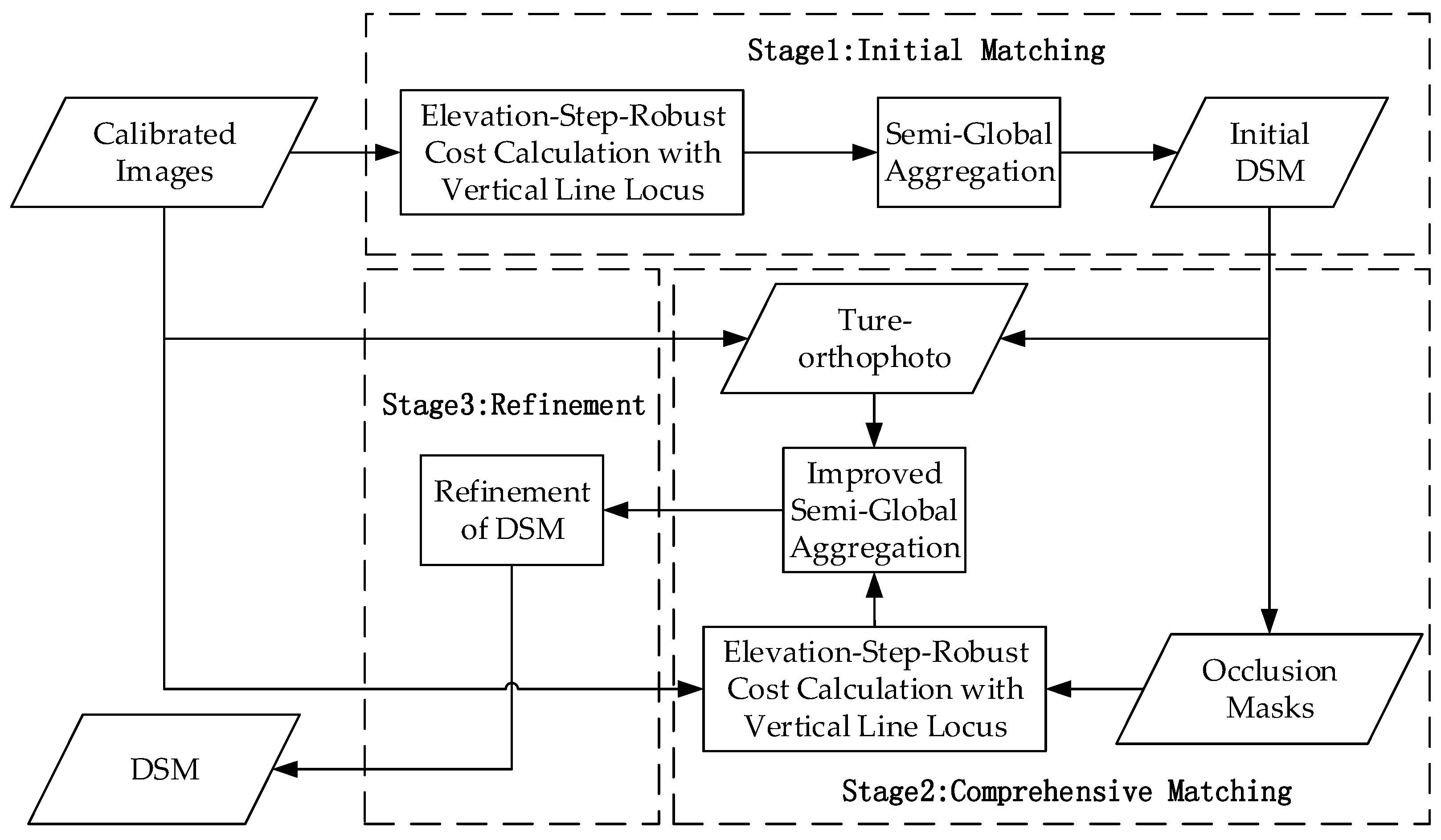
1.2. The Proposed Approach

We think the workflow of DSM generation can be simplified, so we reconsider the issue of DSM generation and focus on how to directly extract an accurate DSM with dense image matching in this paper.
DSM is actually 2.5D, thus there is a strong XY constraint for DSM generation. In other words, only Z is to be estimated with given X, Y. Hence, the generation of a DSM assigns elevation to each of the 2D planar grid points and the elevation of a grid point could be calculated by selecting the best photo-consistency of the visible images (Figure 1). This method is called the vertical line locus method (VLL) in photogrammetry [25]. However, the traditional VLL [25,26] is usually implemented with simple local window based method which tends to fail at regions with discontinuities, weak or repetitive texture, etc. In fact, photo-consistency could be evaluated by a 3D volume in the object space in order to get a robust photo-consistency measure and the surface can be extracted with non-local optimization in a 2D frame to get a smooth 2.5D DSM while keeping the discontinuities.
We propose a novel DSM generation method, called the semi-global vertical line locus matching (SGVLL), which is very different from the current standard workflow to generate a DSM. Basically, the proposed method is an improved version of standard VLL method. Our contribution includes two aspects: (1) A novel workflow for DSM generation is proposed. Compared with the workflow of DSM generation through image matching in the photo space, this one is equivalently robust but much simpler, thus reduces computation redundancy significantly. (2) Improvements including elevation-step-robust cost calculation with handling occlusion and an improved semi-global aggregation with guidance of true-orthophoto, promote the VLL method to be a practical and promising method for DSM generation.

2. Method

A flowchart of the proposed method is presented in Figure 2. The input data for SGVLL is a set of calibrated images while the output is a DSM. SGVLL method has three stages: (1) initial matching; (2) comprehensive matching; and (3) refinement. For the first stage, a robust cost function is calculated with vertical line locus in the object space, achieving a 3D cost matrix which is then semi-globally aggregated in order to generate an initial DSM with the “winner takes all” (WTA) principle. The second stage is comprehensive matching which is the main process of SGVLL. Specifically, the initial DSM is employed to obtain occlusion masks as well as a true-orthophoto. The former is used in cost function to improve photo-consistency measure while the latter is used to guide the semi-global aggregation of the cost matrix, and then WTA principle is employed again to generate a superior DSM. Finally, refinement is used to generate the final DSM with regarding the previous DSM as a 2D float image in the last stage.

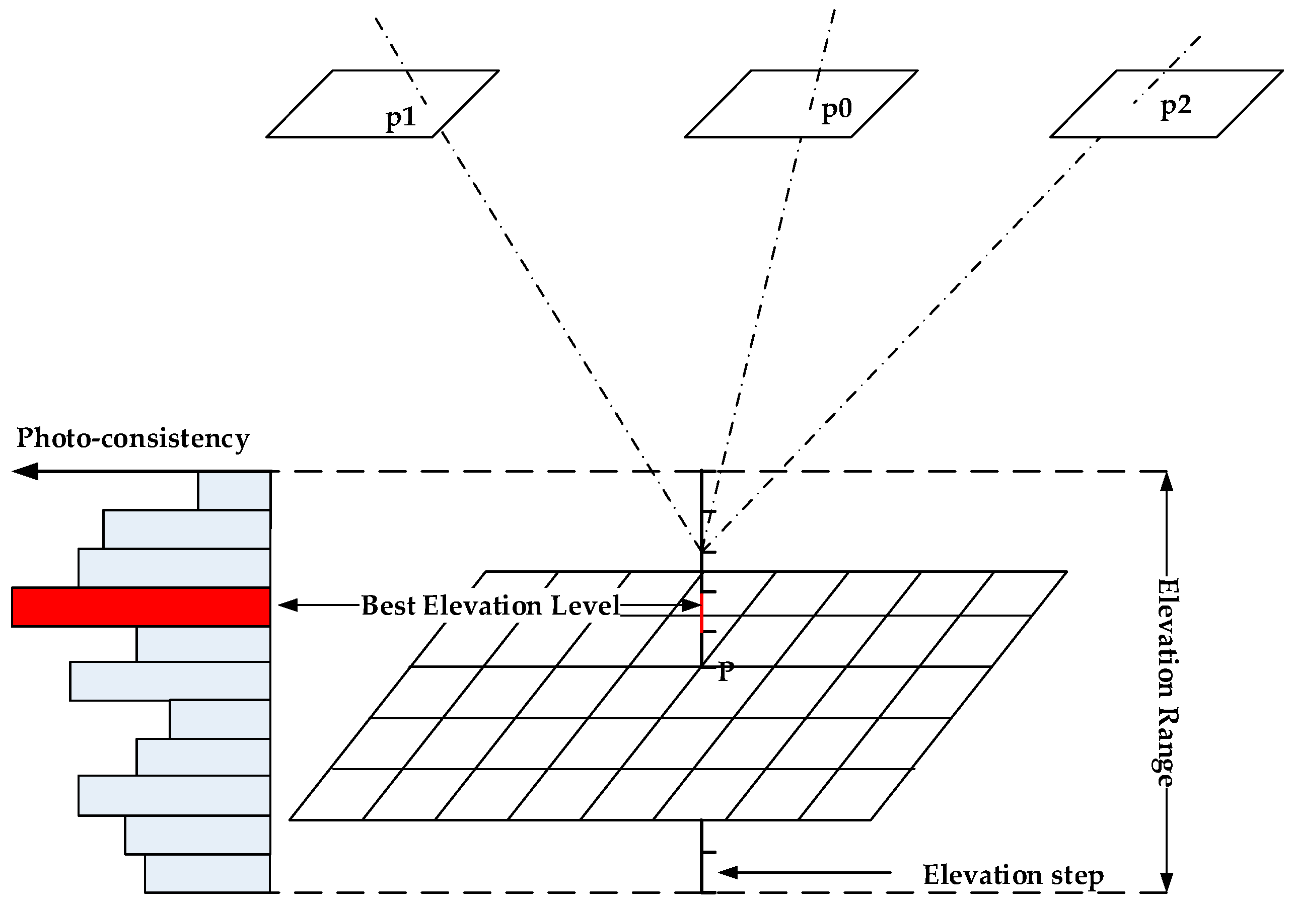
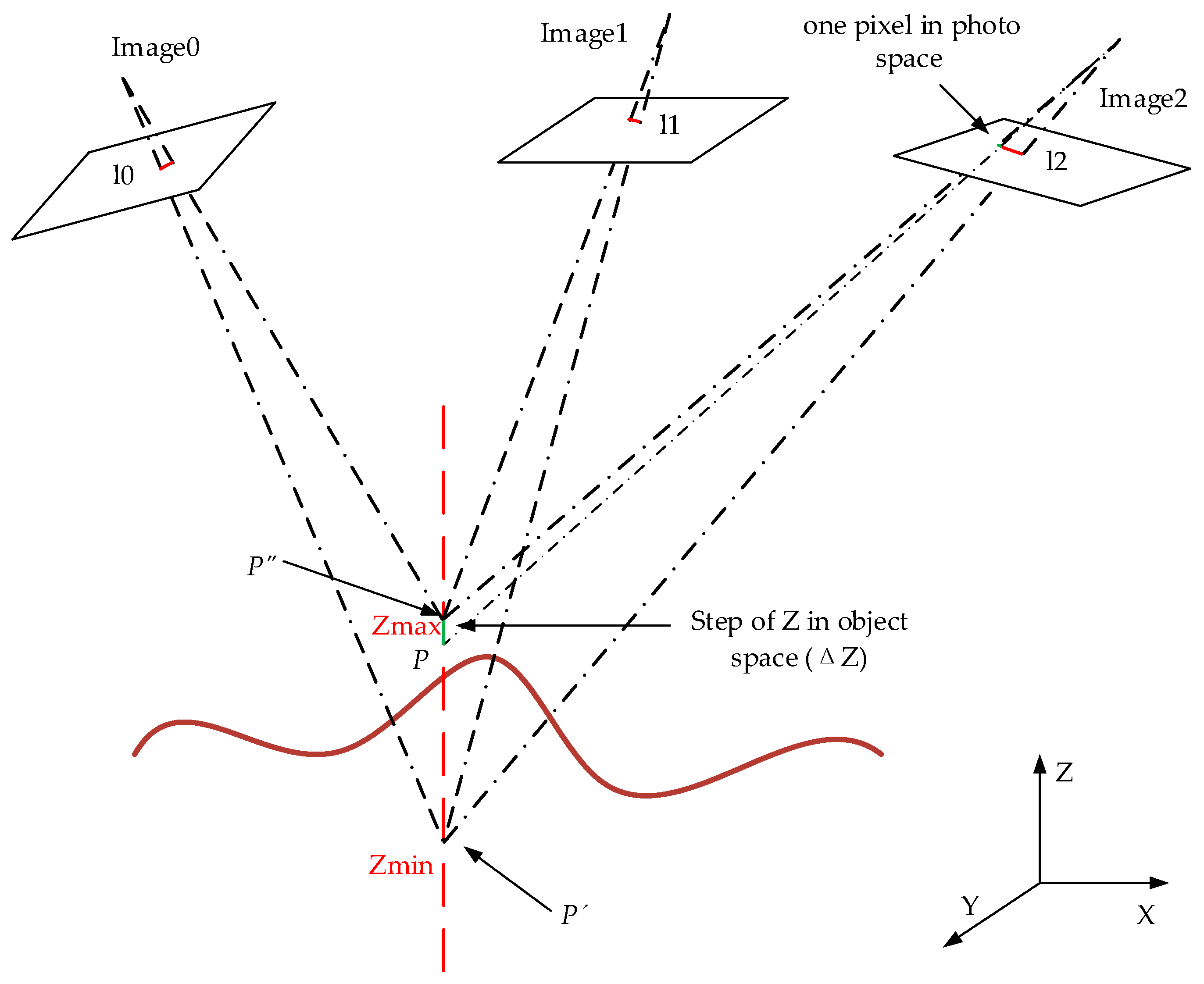
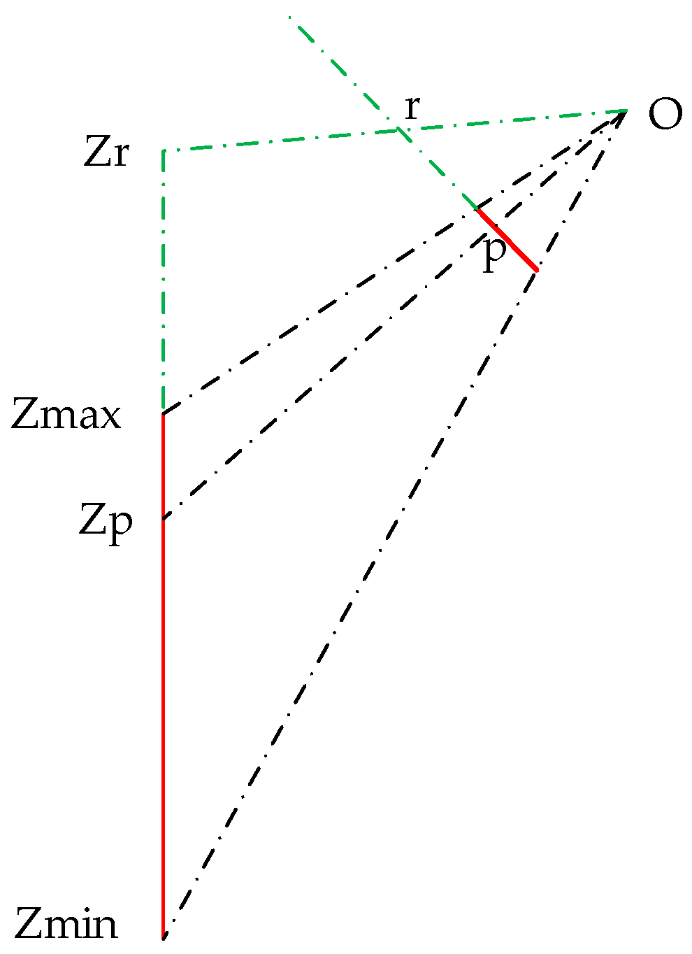
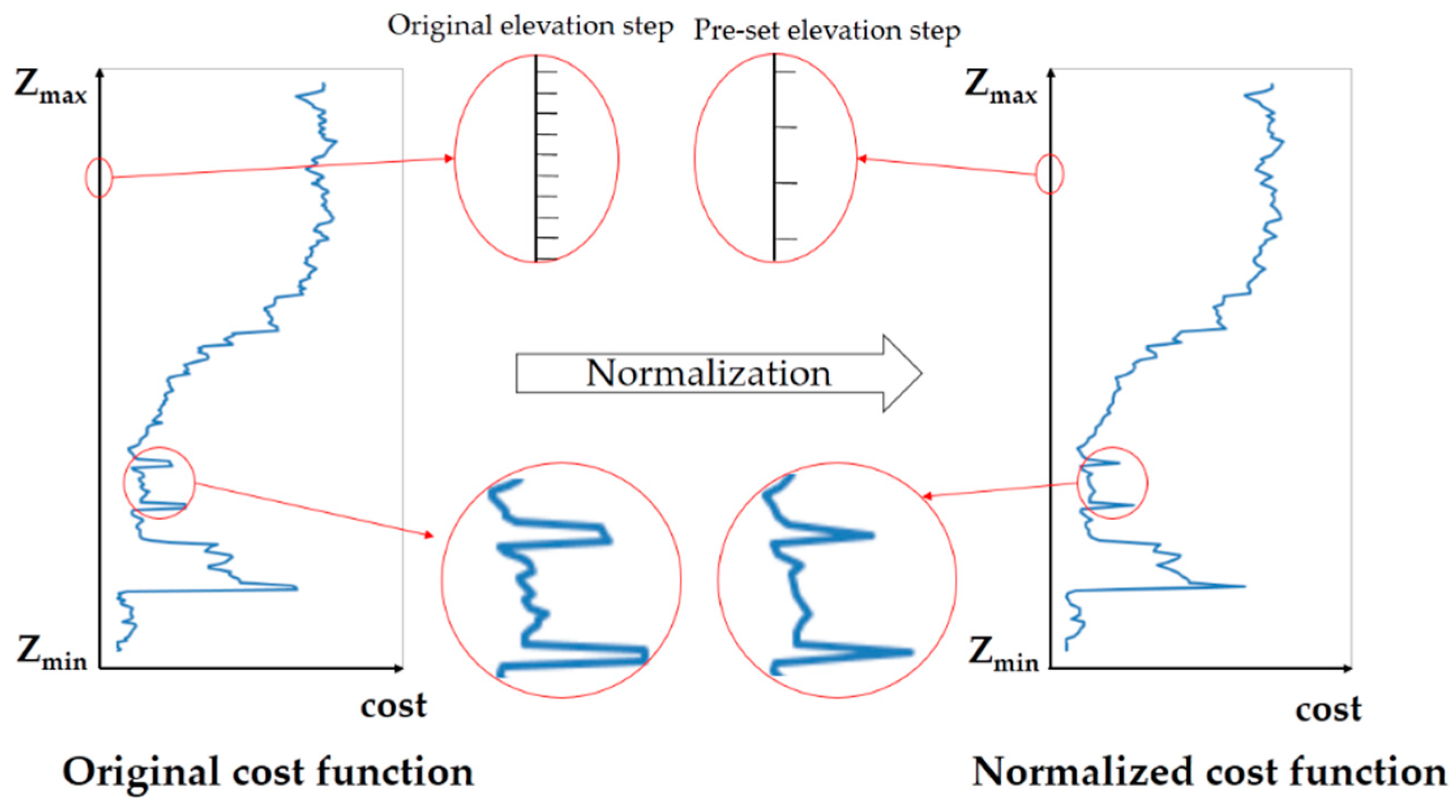
2.1. Elevation-Step-Robust Cost Calculation with Vertical Line Locus

Candidate elevations are given within an elevation range with an elevation step (∆Z, the same below) in VLL method for DSM generation (Figure 1). The elevation step determines how many elevation candidates need to be calculated. The VLL method uses a pre-set fixed step (empirically the ground sampling distance (GSD)), resulting in a poor performance because the small step leads to heavy computation, while the large step leads to a coarse discretization which might discard the projected points on the images of the correct Z value.
Actually, if the projected length of ∆Z on the image is less than one pixel, no correct candidate elevation would be missed. Every pixel in photo space strictly has different GSD due to perspective projection, and every grid point in objet space should have adaptive step to hold a pixel-wise or sub-pixel cost function. Thus, we propose a cost calculation method which is robust to ∆Z for VLL matching. A similar method which is called the point-wise correlation, has been proposed in [27]. In that paper, however, the details about how to calculate ∆Z was not illustrated and the method was different from the vertical line locus method discussed in this paper because points were not selected along the vertical line.
The proposed method consists of three steps: calculation of ∆Z corresponding to one pixel, calculation of cost function, and normalization of cost function. For the first step, given a grid point P(X, Y) and its possible elevation range (Zmin, Zmax), ∆Z corresponding to one pixel in photo space will be computed (Figure 3). Specifically, project the vertical line (from P′(X, Y, Zmin) to P″(X, Y, Zmax)) to all the visible images, thus a locus is generated on each image. Due to perspective projection model, the vertical line locus is a straight line. Then, the minimum pixel-wise back-projected distance of the longest locus will be utilized to calculate ∆Z. According to the theory of cross ratio invariance to perspective projection [28], the minimum pixel-wise projected distance of a locus must be located at P″(X, Y, Zmax). Therefore, the back-projected distance of the pixel projected from P″(X, Y, Zmax) is the minimum elevation step for P which would be utilized as ∆Z.
In detail, as Figure 4 shows, suppose Zr is a point along the vertical line in the object space and r is the projected points of Zr in the photo space. According to the theory of cross ratio invariance, the elevation step can be computed with Equation (1):
Δ Z = λ Z r γ λ Z r + γ 1 ( Z m a x Z m i n ) λ Z r = Z r Z m i n Z m a x Z m i n γ = λ p ( 1 λ r ) λ p λ r
In Equation (1), γ is the cross ratio of (Zmin, Zp, Zmax, Zr), and λ p and λ r are the ratio of projected point p and r, respectively to the locus on the image. For example, if the pixels number of the locus is N, then λ p = 1 N . Note that Δ Z is implicitly independent with Zr because the cross ratio is a projective invariant which intrinsically eliminates Zr with its projected point r. Therefore Zr can be arbitrary and we set Z r = Z m i n + 2 ( Z m a x Z m i n ) .
For the second step, cost of each grid point P(X, Y) is calculated with the following three steps in order to be robust to projection distortion. First, an image with the shortest locus is chosen as the reference image of P. Second, P is projected to the reference image by its object-space coordinate (X, Y) and candidate elevation and a rectangular window (window size is 5 × 5 in this paper) is obtained. The window is then back-projected to the object space, which is further projected to other input images. Third, matching cost of P is given by the average of the zero-mean normalized correlation coefficients (ZNCC) between the reference window and all other windows. Therefore, given a candidate elevation of P, Z P = Z m i n + L p Δ Z , the matching cost C ( P , Z P ) or C ( P , L P ) is calculated with Equation (2).
C ( P , Z P ) = 1 N 1 i N 1 ( 1 Z N C C i ( P , Z P ) ) = C ( P , L P )
where N is the number of the visible images, Z N C C i ( P , Z P ) denotes the zero-mean normalized correlation coefficient of P between the reference image and the i-th image at the elevation Z P (also the elevation level L P ).
For the last step, normalization of cost function is conducted because grid points have various elevation steps, which lead to different cost vector levels of each grid point (Figure 5). If the step is larger than the pre-set value, the latter will be used to calculate the normalized cost vector for the grid point. If not, the calculated cost vector will be firstly min-convoluted [29,30] with a robust function (Equation (3)) and then down-sampled to a normalized cost vector with the pre-set step. The result of min-convolution is the lower envelop of functions by rooting the robust function at all the other levels.
C ( P , L P ) = m i n L P ( C ( P , L P ) + ρ min ( | L P L P | , d ) )
In Equation (3), C ( P , L P ) is the cost of the grid point P at the elevation level L P .

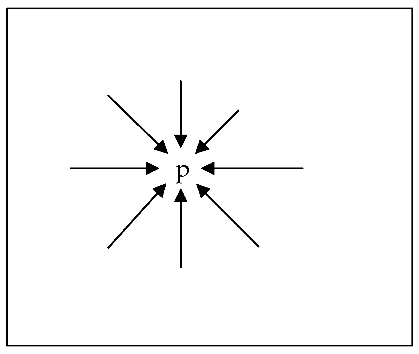
2.2. Initial DSM Generation with Semi-Global Aggregation

Semi-global cost aggregation is originally used in binocular stereo matching [2]. The semi-global aggregation function is given by 1-D energy function with piecewise smooth constraint. As shown in Figure 6, pixel-wise cost is aggregated for each pixel from at least eight directions independently. Then, optimal disparity of each point is obtained by the WTA principle.
We replace the disparity in binocular stereo matching with the elevation level in the energy function, and then employ the semi-global aggregation and WTA to extract an initial DSM from the cost matrix in the object space. Specifically, the energy function is Equation (4) which depends on the elevation label field L.
E ( L ) = P ( C ( P , L P ) + Q N P P 1 T [ | L P L Q | = 1 ] + Q N P P 2 T [ | L P L Q | > 1 ] ) T [ x ] = { 1 ,   x = t r u e 0 ,   x = f a l s e
where Q is the neighborhood point of P, and P1 and P2 are constants, which are the penalties for level change. Finally, the optimal elevation level of P is assigned by the WTA principle, with which the elevation Z P can be estimated with Equation (5).
Z P = Δ Z argmin L P   E ( P , L P ) + Z m i n

2.3. Cost Function Calculation with Handling Occlusion

The DSM generated with the above steps would be smooth with edge reserved. However, mismatching remarkably appears around high buildings due to occlusion (Figure 7). Such problem can be solved by taking visibility into consideration during cost calculation.
Occlusion is one of the key reasons of poor matching results. Basically, there are two types of methods that could be used to solve this problem: the first is outlier-based approaches which regard occlusion as outliers and employ robust photo-consistency calculating methods, such as shiftable windows, sum of normalized cross-correlation (SNCC), etc. [16,31]. The second is geometric approaches, which explicitly detect occlusion and predict visibility in order to improve photo-consistency measure [17,32]. The first type is simple, but has relatively poor result. The second type is relatively complex, but holds better performance, which is chosen in our method.
Angle based spiral sweep method [33] is employed to detect occlusion with the initial DSM. By projecting grid points to all the images, an occlusion mask which encodes the visibility of grid points, is generated for each image. Cost matrix will be calculated again with occlusion masks in “comprehensive matching” stage (Figure 2). According to Equation (2), if a grid point is occluded on an image, this image would be neglected when calculating the matching cost of a grid point. If the number of visible images for a grid point is less than 2, the grid point will be regarded as invisible point and neglected in the sequent processes. Although the initial DSM is not quite accurate, which causes inaccuracy in the occlusion mask, it can still eliminate most mismatches. The small amount of remaining errors can be removed by semi-global aggregation.

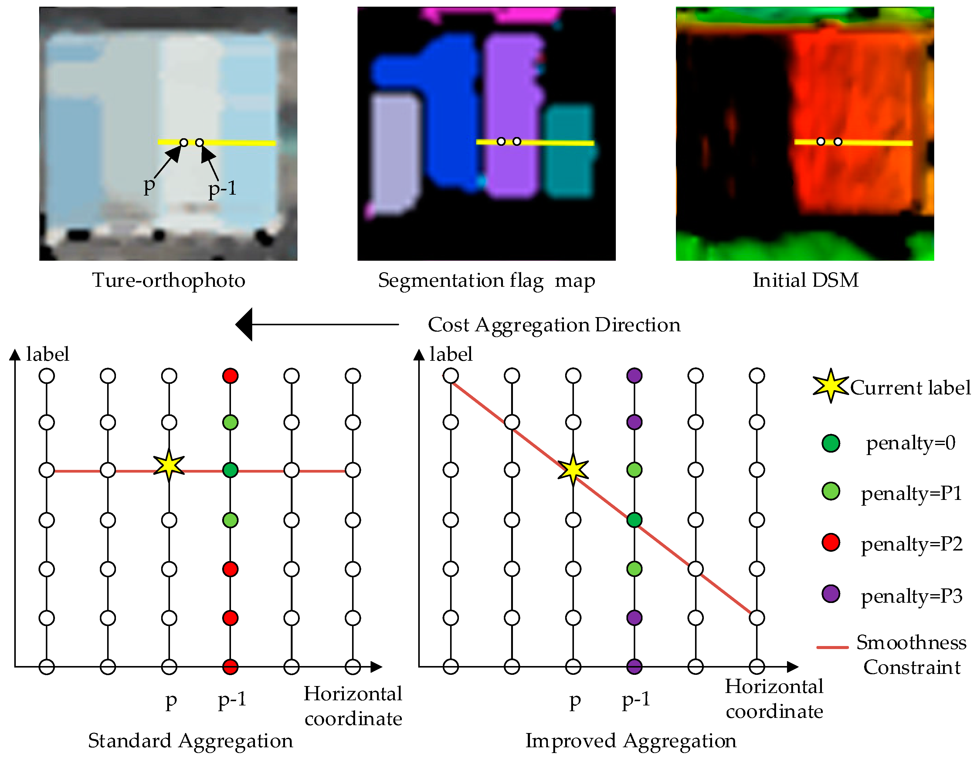
2.4. Improved Semi-Global Aggregation with Guidance of True-orthophoto

Semi-global aggregation works successfully at texture abundant regions which would generate smooth and edge preserved DSM. However, it tends to fail at weak texture regions, especially at slanted planes with weak texture. In order to improve matching results at weak texture regions, more prior knowledge should be used, such as gradient of intensity, segmentation of image, an initial DSM, etc. In fact, many binocular stereo matching algorithms using image guided aggregation have been developed. For example, SGM [2] uses an adaptive P2 calculated with the gradient of intensity at the local pixel; cost filtering method [9] uses the image based filter kernel to guide the filtering of cost volume; and MST method [4] constructs the minimum spanning tree on the image, according to which cost is aggregated.
Inspired by the above methods, we employ the image guided aggregation in this paper. However, there is no reference image for the object-space based cost matrix. Therefore, we propose the true-orthophoto guided aggregation method, which generates a true-orthophoto [33] to guide the aggregation of the cost matrix. Note that the true-orthophoto has the same GSD with the initial DSM. Before the guidance, the true-orthophoto is preprocessed as follows: First, those grid points with high cost will get invalid values on the true-orthophoto. The cost threshold T_c for processing is 0.95 in this paper. Second, the true-orthophoto is filtered by a median filter. Median filter window size is 3 × 3 in this paper.
The true-orthophoto guided aggregation is as follows: First, the true-orthophoto is segmented by region growing algorithm, and each pixel p is assigned a segmentation label Sp. Second, segmented pieces with large pixel count (threshold of pixel count T_seg is 100 in this paper) are regarded as weak texture regions. Pixels belonging to these pieces would be labeled with positive number, whereas other pieces would be labeled as −1. Note that the pixels with invalid value would also be labelled as −1. An adaptive smoothness constraint is then used on these labeled pixels during the true-orthophoto guided cost aggregation.
Meanwhile, as shown in Equation (4), the smoothness constraint is actually a horizontal constraint. The above adaptive smoothness constraint might result in fronto-parallel bias at slanted planes with weak texture. To avoid this problem, a factor derived from the initial DSM is added in the energy function. Therefore, the final energy function for the improved cost aggregation is as follows:
E ( L ) = P ( C ( P , L P ) + Q N P P 1 T [ | L P L Q Δ L | = 1 ] + Q N P ρ   T [ | L P L Q Δ L | > 1 ] ) Δ L = { L P L Q ,   i f   | L P L Q | < τ τ ,   o t h e r w i s e ρ = { P 3 ,   S p = S q 1 P 2 ,   o t h e r w i s e
In Equation (6), L P and L Q are labels on initial DSM corresponding to the grid points P and Q, respectively. τ is a constant for controlling the slope consistency with the initial DSM. ρ is the new penalty in place of P 2 of Equation (4). p and q are pixels on the true-orthophoto corresponding to the grid points P and Q, respectively. Sp and Sq are segment flags of p and q, respectively. Note that P3 must be larger than P2 in order to encourage stronger smoothness at weak texture regions.
Compared with Equation (4), which is used in standard cost aggregation, Equation (6) uses a larger penalty at weak texture regions and it will improve the matching results at regions with weak texture. Besides, Equation (6) transforms the horizontal smoothness into overall smoothness according to the initial DSM, which can remove fronto-parallel bias of slanted planes effectively. Actually, Equation (4) is a special case of Equation (6) with setting Δ L = 0 and ρ = P 2 .
The differences between standard aggregation and improved aggregation are illustrated in Figure 8. As mentioned in Section 2.2, pixel-wise cost is aggregated for each pixel from at least eight directions independently. Figure 8 shows an aggregation path, along which cost of the current label at p is being aggregated. The standard aggregation uses horizontal smoothness without considering weak texture. The improved aggregation adopts the smoothness constraint according to initial DSM and uses adaptive penalties according to the segmentation flag map derived from the true-orthophoto.
At last, it can be seen that the new energy function would be affected by mistakes in the initial DSM and true-orthophoto in terms of Δ L and ρ . The influence of the initial DSM on Δ L can be well controlled by using a small τ , such as 3 in this paper. Regarding ρ , the influence of the mistakes in the true-orthophoto is very limited because only the weak texture regions of true-orthophoto are detected and used to improve the results, and these regions tend to have few mistakes after preprocessing of the true-orthophoto.

2.5. Refinement of the DSM

Finally, the generated DSM needs to be refined because it inevitably has outliers and its elevation value is coarse due to previous discretization. First, the DSM is regarded as a 2D float image and filtered with a median filter. Then, parabola interpolation [34] is used to refine the elevation of each point independently. Parabola interpolation is conducted by fitting a parabola curve using the aggregated cost of optimal elevation level and its left and right side elevation levels. The sub-level (l*) corresponding to the extreme of the parabola curve is taken as the final elevation level, with which the final elevation is achieved (Equation (7)).
L P = L P 0.5 c 0 c 1 c 1 + c 2 c 0 Z P = Δ Z L P + Z m i n
where c0, c1, and c2 are aggregated cost for level L P , L P 1 , and L P + 1 , respectively; c* is the minimal cost interpolated from parabola curve; and L P is the sub-level corresponding to c*.

3. Results

3.1. Data and Methods

The main experimental data was 28 nadir images of SWDC-5, which covered about 1 km2 area within Wuhan University, China (Figure 9). SWDC-5 is an oblique aerial camera system produced by GEO-VISION Co., Ltd., China. The nadir camera has 8176 × 6132 pixels image format and 6 µm physical pixel size. Flying height of this data was 950 m with focal length of 50.698 mm. The GSD of imagery was 0.1 m. A DSM interpolated with LiDAR, which has a GSD of 1m, was given as reference data covering the same geographical area.
Besides, the dense image matching benchmark provided by the European Spatial Data Research Organization (EuroSDR) was used as supplementary experimental data, which consisted of two testing sites. The first testing site was located at München and covered a built-up urban area. The second testing site was located at Vaihingen/Enz and covered a semi-rural area at undulating terrain. For each testing site, aerial images were used to generate DSMs using eight software packages, from which a median DSM was generated and used as reference data. More details about the benchmark can be found in [35].
We implemented SGVLL with C++ language and run the program on a PC with an Intel(R) Core(TM) i7-4790 CPU. The parameters used in this paper were: P 1 = 0.3, P 2 = 1.2, P 3 = 2.0, τ = 3, T_seg = 100, and T_c = 0.95. In the following experiments, Section 3.2, Section 3.3 and Section 3.4 were designed for verifying the effectiveness of the proposed methods while Section 3.5 was comparative experiment for quality assessment of generated DSMs.
For quality assessment, the DSMs generated by SGVLL were compared with both reference data and the DSMs generated by commercial software SURE. SURE is a state-of-the-art software for DSM generation and 3D reconstruction which was developed by University of Stuttgart, Germany. The core algorithm of SURE is SGM, which produces DSM by interpolating 3D point clouds generated by merging large number of binocular SGM results. The proposed SGVLL was somewhat similar to SGM, but directly conducted in the object space. Therefore, a comparison between SURE and SGVLL was necessary. Before quality assessment, we first generated DSMs with the same GSD as the input images; then the DSMs were resampled in order to keep the same GSD with the reference data.
In the following experiments, some of the figures for showing DSMs (without color bar) used a default color scale which was consistent with reference data (Figure 9b), and other figures showed DSMs with adaptively scaled color range (with color bars) in order to show more details.

3.2. Experiment on Elevation-Step-Robust Cost Calculation

In order to verify the advantage of the proposed elevation-step-robust cost calculation, both traditional method (the cost calculation method of the standard VLL) using GSD as the constant elevation step and proposed method using an adaptive elevation step, were employed to generate DSMs with different GSDs, namely 0.5 m, 5 m, and 10 m. As shown in Figure 10, the first row is the results of the traditional method, and the second row displays DSMs generated by the proposed method. When the GSD was 0.5 m, both methods achieved good results. When the GSD was 5 m, result of the traditional method degenerated significantly, especially at the high building area at the left bottom of the Figure 10b. When the GSD was 10 m, result of the traditional method was generally wrong, which was not able to depict the terrain surface, while the result of the proposed method was generally correct, though degeneration of details existed.

3.3. Experiment on SGVLL with Handling Occlusion

This section was designed to verify the effectiveness of handling occlusion. Figure 11 denotes the matching cost maps of the DSMs without and with the occlusion detection. It can be seen from Figure 11a that the cost (See Equation (2)) was very high before occlusion detection, especially around high buildings, which indicates there were lots of matching errors. These errors were removed obviously with occlusion detection in Figure 11b. Quantitatively, the very high cost percentage (larger than 0.95) decreased from 4.58% to 2.32% with handling occlusion.
Moreover, four subsets of the DSM were selected to denote the effectiveness of occlusion detection in detail. DSMs generated without and with occlusion detection are shown in Figure 12. It is noteworthy that points with very high matching cost (larger than 0.95) have been removed. It can be seen that the number of points removed from the DSM with occlusion detection was far less than that without occlusion detection.

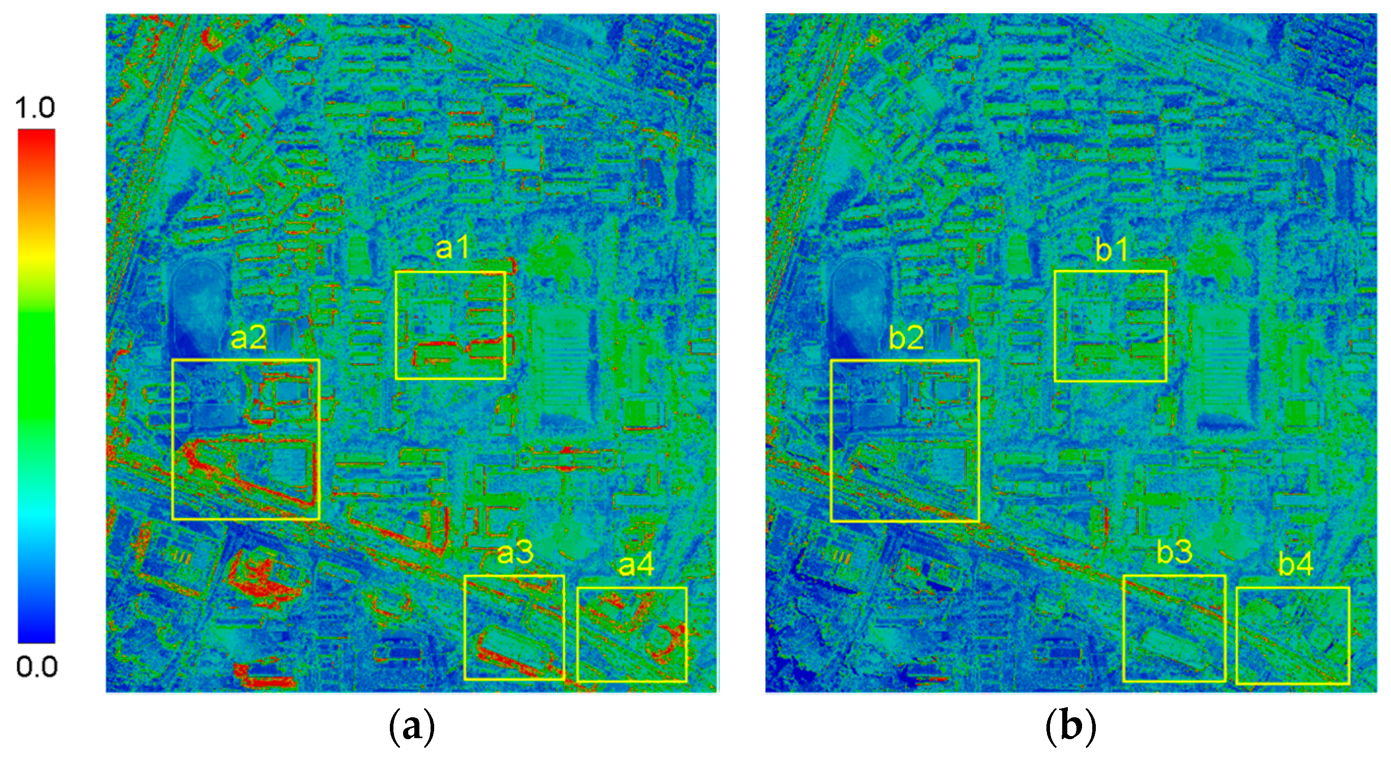
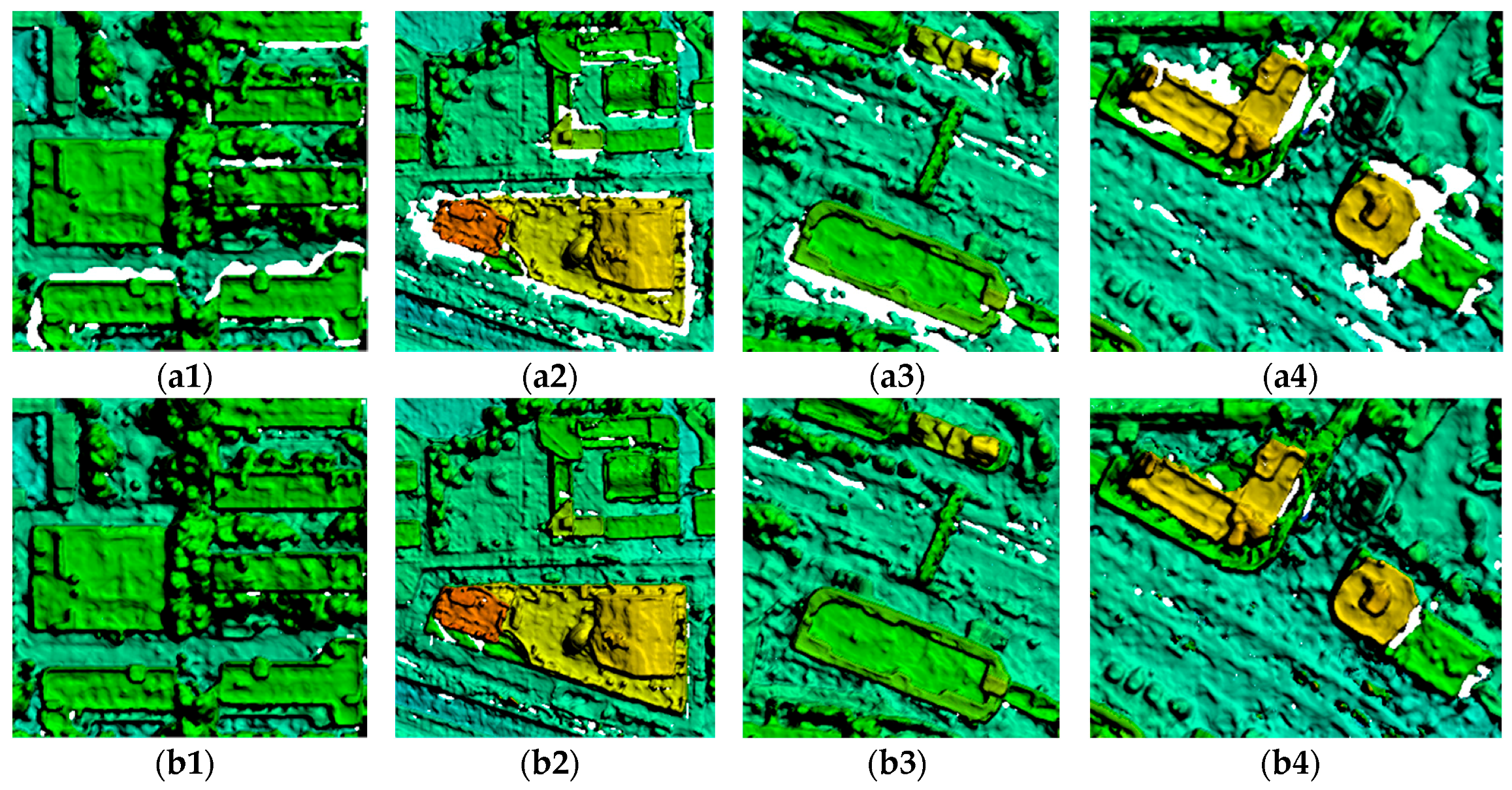
3.4. Experiment on Improved Semi-Global Aggregation

The improved semi-global aggregation was expected to improve the performance at weak texture regions and slanted planes, which was tested in this section.
Firstly, the effect of true-orthophoto guidance on weak texture regions was tested. In Figure 13, the first and the second columns show the true-orthophotos and segmentation flag maps, respectively. The third column shows the DSMs generated without true-orthophoto guidance on which mismatches tended to happen in weak texture regions, including lake (the first row), swimming pool (the second row) and building roofs (the last two rows). The fourth column shows the DSMs generated with the true-orthophoto guidance where most of the mismatches have been removed.
Secondly, the effect on slanted planes using the improved semi-global aggregation was tested. As shown in Figure 14a–c, the DSMs generated by standard semi-global aggregation described in Section 2.2. It can be seen that all these DSMs had obvious fronto-parallel bias at slanted planes. Figure 14d–f shows the DSMs generated by the improved semi-global aggregation, on which the fronto-parallel bias had been removed.

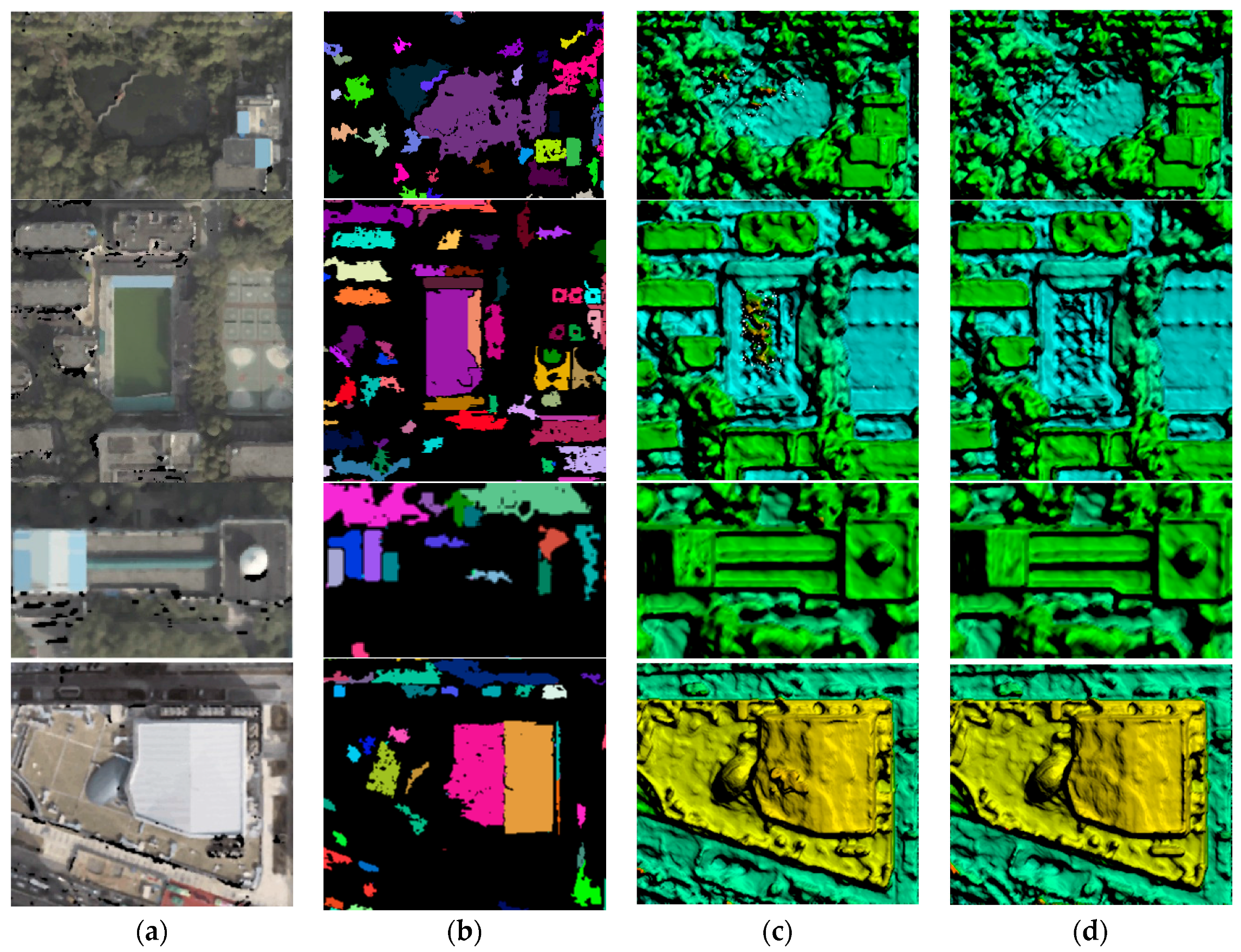
3.5. DSM Quality Assessment

Visually comparative experiments were firstly conducted. Figure 15 shows the DSMs of Wuhan University generated by LiDAR, SURE and SGVLL. It seems that SGVLL achieved smoother and slightly better results than SURE. The second row of Figure 15 reveals that result of SGVLL was closer to the DSM generated by LiDAR. Three places of the subset should be noticed. Firstly, DSM of LiDAR was wrong at the lake in the left part of the subset, which was correctly generated by SURE and SGVLL. Secondly, at the middle bottom of the subset where there are big trees and shadows in the images, there are many matching errors on DSM generated by SURE while the DSMs by SGVLL and LiDAR were consistent. Lastly, the playground generated by SGVLL was smoother than that by SURE. The third row depicts the result of DSM at regions with dense buildings, which are difficult for stereo matching mainly because of the hardness of preserving the edges. Both SURE and SGVLL achieved good results at this region. The fourth row shows results of DSM at high build-ups and street regions. Due to projection deformation, occlusion and moving objects, it was the most challenging part in dense image matching. It shows that SURE and SGVLL had similar results, while the result of SGVLL was smoother.
Figure 16 shows the results on München subset. Generally, SGVLL achieved performance close to SURE. Compared with SURE, the DSM generated by SGVLL was smoother and some details disappeared (red rectangles) but some burrs were removed (yellow rectangles).
Figure 17 shows the results on Vaihingen/Enz subset. Generally, SURE and SGVLL achieved similar performance. Compared with SURE, the DSM generated by SGVLL was smoother and some burrs were removed (yellow rectangles). However, as shown in red rectangle, the river had weak textures, where some mistakes happened on the DSM generated by SGVLL.
We conducted quantitative evaluation on generated DSMs against the reference data for all the testing sites. Firstly, the residual errors of generated DSMs against the reference data were collected. It is noteworthy that the residual errors would be calculated with elevations of SURE and SGVLL if both residual errors against reference data were too large (threshold was 10 m in this paper). In this way, some remarkable changes and errors existing in the reference data would not affect the quantitative assessment. Based on the residual errors, three indicators were calculated, namely, root mean square error (RMSE), mean error (ME), and time consumption. The results are shown in Table 1. Regarding Wuhan University testing, SGVLL outperformed SURE in terms of both RMSE and ME. The results on München and Vaihingen/Enz subsets suggested that SURE had lower RMSEs but slightly higher MEs than SGVLL. For all the testing sites, the time consumption of SGVLL was significantly less than SURE.

4. Discussion

4.1. Advancements of the Proposed Method

Different with most of photo-space-based DSM generation methods which tend to suffer from process complexity and computation redundancy, this paper introduces a direct DSM generation approach, namely SGVLL, aiming at conducting DSM generation with dense matching in the object space directly.
SGVLL was based on the traditional VLL method [25,26] but three improvements were performed and verified by experimental results. First, as shown in Section 3.2, we confirm that the elevation-step-robust cost calculation was effective to improve the poor robustness of elevation step in VLL method since the proposed method achieved much better accuracy and robustness than VLL method with respect to the elevation step. Second, due to the usage of the initial DSM, the method of handling occlusion in SGVLL was straight-forward but effective since it can remove most of themismatches caused by occlusion as shown in Section 3.3. Third, the experimental results in Section 3.4 demonstrated that the improved semi-global aggregation was also effective since the DSMs at both weak texture regions and slanted planes were improved significantly and robustly.
It can be seen from the results in Section 3.5 that the DSM quality generated by SGVLL achieved a performance very close to that by SURE, a successful software for DSM generation and 3D reconstruction. Based on the work of Haala [35], it was adequate to use the DSM generated by SURE as the state-of-the-art performance. In addition, the experiments included visual comparison and quantitative assessment using the reference data while the testing datasets included built-up urban area and semi-rural area at undulating terrain. Quantitative assessment showed that SGVLL performed better than SURE in Wuhan University site but worse than SURE in the other two sites. This might be caused by the resolution of reference data. For Wuhan University site, the reference data was a DSM with a GSD of 1 meter, thus the reference data had a lower resolution (GSD) than the generated DSMs by SGVLL and SURE. However, DSMs which had the same GSD with the generated DSMs by SGVLL and SURE, were used as reference data for the other two sites. SGVLL cannot reconstruct some details, thus decreased the accuracy when the reference data hold these details. However, the success in Wuhan University of SGVLL suggested that SGVLL could generate a more accurate DSM than SURE when the required resolution of DSM was lower. In summary, the experimental results in Section 3.5 can draw a general conclusion that the proposed SGVLL achieves performance very close to the state-of-the-art.
As shown in Section 3.5, the proposed SGVLL requires less time for processing because it directly generates DSM by multi-view matching while SURE requires binocular stereo matching, disparity map fusion, point cloud merging, and DSM interpolation. Moreover, the processing unit of binocular stereo matching is photo-space-based stereo model, which leads to computational redundancy. For example, regarding the experimental data of Wuhan University, 41 valid stereo models were generated by SURE and semi-global optimization was employed for 82 times since “Left-Right-Check” strategy was included in the binocular stereo matching. However, SGVLL needs only twice semi-global optimization in object space. In fact, although the current program of SGVLL has not been fully optimized, the time consumption was far less than SURE.

4.2. Limitations of the Proposed Method

According to the experimental results, SGVLL tended to generate an over-smooth DSM, on which some details disappeared. The reason included two aspects: first, we had used a strong smoothness constraint (by setting P 2 as a large value) in SGVLL to keep the DSM from outliers; second, SGVLL cannot reconstruct objects which had a size of GSD or even smaller because a regular grid was pre-set based on GSD. Besides, as shown in Figure 17, the usage of true-orthophoto in SGVLL did not completely solve the problem in large-area regions with weak texture.

5. Conclusions

This paper proposes a novel DSM generation approach called the SGVLL, which implements multi-view stereo matching directly in the object space. Compared with the photo-space based DSM generation methods, SGVLL is simpler and reduces computational redundancy significantly. Compared with the standard VLL, SGVLL can obtain a much superior DSM effectively and robustly with the improvements including an elevation-step-robust cost calculation with handling occlusion and an improved semi-global aggregation with guidance of true-orthophoto. Experimental results demonstrate that all of the proposed improvements are effective and SGVLL achieves performance very close to the state-of-the-art with much less time consumption.
In the future work, a method for regaining more details, such as the coarse-to-fine strategy, is needed to be investigated and employed in SGVLL. Besides, how to extract an accurate DSM for large-area regions with weak texture is worth further study.

Acknowledgments

This work was supported by National Natural Science Foundation of China with project number 41571434 and 41322010. We appreciate Mathias Rothermel and Konrad Wenzel to provide SURE for non-commercial use which allows us to conduct the comparison experiments. Many thanks also go to Professor Haala and his co-members for providing the benchmark on high density image matching for DSM generation. We also thank the anonymous reviewers and the Editor of the journal for their useful comments.

Author Contributions

Yanfeng Zhang and Yongjun Zhang conceived the study and designed the experiments; Yanfeng Zhang and Delin Mo performed the experiments; Yanfeng Zhang wrote the paper; and Yi Zhang and Xin Li helped to prepare the manuscript. All authors read and approved the final manuscript.

Conflicts of Interest

The authors declare no conflict of interest.

Abbreviations

The following abbreviations are used in this manuscript:
DSMDigital surface model
SGVLLSemi-global vertical line locus
GSDGround sampling distance
ZNCCZero-mean normalized correlation coefficient
WTAWinner takes all

References

  1. Scharstein, D.; Szeliski, R. A taxonomy and evaluation of dense two-frame stereo correspondence algorithms. Int. J. Comput. Vis. 2002, 47, 7–42. [Google Scholar] [CrossRef]
  2. Hirschmüller, H. Stereo processing by semiglobal matching and mutual information. IEEE Trans. Pattern Anal. Mach. Intell. 2008, 30, 328–341. [Google Scholar] [CrossRef] [PubMed]
  3. Yoon, K.; Kweon, I.S. Adaptive Support-Weight approach for correspondence search. IEEE Trans. Pattern Anal. Mach. Intell. 2006, 28, 650–656. [Google Scholar] [CrossRef] [PubMed]
  4. Yang, Q. A Non-local cost aggregation method for stereo matching. In Proceedings of the IEEE International Conference on Computer Vision and Pattern Recognition, Providence, RI, USA, 16–21 June 2012; pp. 1402–1409.
  5. Bleyer, M.; Gelautz, M. A layered stereo matching algorithm using image segmentation and global visibility constraints. ISPRS J. Photogramm. Remote Sens. 2005, 59, 128–150. [Google Scholar] [CrossRef]
  6. Xu, S.B.; Zhang, F.H.; He, X.F.; Shen, X.K.; Zhang, X.P. PM-PM: PatchMatch with potts model for object segmentation and stereo matching. IEEE Trans. Image Process. 2015, 24, 2182–2196. [Google Scholar] [PubMed]
  7. Hirschmüller, H.; Scharstein, D. Evaluation of stereo matching costs on images with radiometric differences. IEEE Trans. Pattern Anal. Mach. Intell. 2009, 31, 1582–1599. [Google Scholar] [CrossRef] [PubMed]
  8. Tombari, F.; Mattoccia, S.; Stefano, L.D.; Addimanda, E. Classification and evaluation of cost aggregation methods for stereo correspondence. In Proceedings of the IEEE International Conference on Computer Vision and Pattern Recognition, Anchorage, AK, USA, 23–28 June 2008; pp. 1–8.
  9. Hosni, A.; Rhemann, C.; Bleyer, M.; Rother, C.; Gelautz, M. Fast Cost-volume filtering for visual correspondence and beyond. IEEE Trans. Pattern Anal. Mach. Intell. 2013, 35, 504–511. [Google Scholar] [CrossRef] [PubMed]
  10. Boykov, Y.; Kolmogorov, V. An experimental comparison of min-cut/max-flow algorithms for energy minimization in vision. IEEE Trans. Pattern Anal. Mach. Intell. 2004, 26, 1124–1137. [Google Scholar] [CrossRef] [PubMed]
  11. Newcombe, R.; Izadi, S.; Hilliges, O.; Molyneaux, D. KinectFusion: Real-time dense surface mapping and tracking. In Proceedings of the International Symposium on Mixed and Augmented Reality, Basel, Switzerland, 26–29 October 2011.
  12. Rumpler, M.; Wendel, A.; Bischof, H. Probabilistic range image integration for DSM and true-orthophoto generation. In Proceedings of the Scandinavian Conference on Image Analysis, Espoo, Finland, 17–20 June 2013.
  13. Jacquet, B.; Hane, C.; Angst, R.; Pollefeys, M. Multi-body depth-map fusion with non-intersection constraints. In Proceedings of the European Conference on Computer Vision, Zurich, Switzerland, 6–12 September 2014.
  14. Seitz, S.; Curless, B.; Diebel, J.; Scharstein, D.; Szeliski, R. A Comparison and evaluation of multi-view stereo reconstruction algorithms. In Proceedings of the Conference on Computer Vision and Pattern Recognition, New York, NY, USA, 17–22 June 2006.
  15. Kolmogorov, V.; Zabih, R. Multi-camera scene reconstruction via graph cuts. In Proceedings of the European Conference on Computer Vision, Copenhagen, Denmark, 28–31 May 2002.
  16. Zhang, L. Automatic Digital Surface Model (DSM) Generation from Linear Array Images; Swiss Federal Institute of Technology: Zurich, Switzerland, 2004. [Google Scholar]
  17. Zhu, Z.K.; Stamatopoulos, C.; Fraser, C.S. Accurate and occlusion-robust multi-view stereo. ISPRS J. Photogramm. Remote Sens. 2015, 109, 47–61. [Google Scholar] [CrossRef]
  18. Seitz, S.M.; Dyer, C.R. Photorealistic scene reconstruction by voxel coloring. Int. J. Comput. Vis. 1999, 35, 151–173. [Google Scholar] [CrossRef]
  19. Vogiatzis, G.; Torr, P.; Cipolla, R. Multi-view stereo via volumetric graph-cuts. In Proceedings of the IEEE International Conference on Computer Vision, Beijing, China, 15–21 October 2005.
  20. Kutulakos, K.N.; Seitz, S.M. A theory of shape by space carving. Int. J. Comput. Vis. 2000, 38, 199–218. [Google Scholar] [CrossRef]
  21. Jin, H.L.; Soatto, S.; Yezzi, A.J. Multi-view stereo reconstruction of dense shape and complex appearance. Int. J. Comput. Vis. 2005, 63, 175–189. [Google Scholar] [CrossRef]
  22. Furukawa, Y.; Ponce, J. Accurate, dense, and robust multiview stereopsis. IEEE Trans. Pattern Anal. Mach. 2010, 32, 1362–1376. [Google Scholar] [CrossRef] [PubMed]
  23. Shan, Q.; Curless, B.; Furukawa, Y.; Hernandez, C.; Seitz, S.M. Occluding contours for multi-view stereo. In Proceedings of the IEEE International Conference on Computer Vision and Pattern Recognition, Columbus, OH, USA, 23–28 June 2014.
  24. Shao, Z.; Yang, N.; Xiao, X.; Zhang, L.; Peng, Z. A multi-view dense point cloud generation algorithm based on low-altitude remote sensing images. Remote Sens. 2016, 8, 381–397. [Google Scholar] [CrossRef]
  25. Linder, W. Digital Photogrammetry-A Practical Course; Springer: Berlin/Heidelberge, Germany, 2006. [Google Scholar]
  26. Ji, S.; Fan, D.Z.; Zhang, Y.S.; Yang, J.Y. MVLL Multi-image matching model and its application in ADS40 linear array images. Geomat. Inf. Sci. Wuhan Univ. 2009, 34, 28–31. [Google Scholar]
  27. Santel, F.; Linder, W.; Heipke, C. Stereoscopic 3D-image sequence analysis of sea surfaces. Int. Arch. Photogramm. Remote Sens. Spat. Inf. Sci. 2004, XXXI-B5, 708–712. [Google Scholar]
  28. Hartley, R.; Zisserman, A. Multiple View Geometry in Computer Vision; Cambridge University Press: Cambridge, UK, 2004. [Google Scholar]
  29. Angulo, J. (Max, min)-convolution and mathematical morphology. In Proceedings of the International Symposium on Mathematical Morphology, Reykjavik, Iceland, 27–29 May 2015; pp. 485–496.
  30. Tan, X.; Sun, C.; Wang, D.; Guo, Y.; Pham, T.D. Soft cost aggregation with multi-resolution fusion. In Proceedings of the European Conference on Computer Vision, Zurich, Switzerland, 6–12 September 2014; pp. 17–32.
  31. Kang, S.; Szeliski, R.; Chai, J. Handling occlusions in dense multi-view stereo. In Proceedings of the IEEE International Conference on Computer Vision and Pattern Recognition, Kauai, HI, USA, 8–14 December 2001; pp. 103–110.
  32. Zeng, G.; Paris, S.; Quan, L.; Sillion, F. Progressive surface reconstruction from images using a local prior. In Proceedings of the IEEE International Conference on Computer Vision, Beijing, China, 15–21 October 2005; pp. 1230–1237.
  33. Habib, A.F.; Kim, E.M.; Kim, C.J. New methodologies for true orthophoto generation. Photogramm. Eng. Remote Sens. 2007, 73, 25–36. [Google Scholar] [CrossRef]
  34. Céspedes, I.; Huang, Y.; Ophir, J.; Spratt, S. Methods for estimation of subsample time delays of digitized echo signals. Ultrason. Imaging 1995, 17, 142–171. [Google Scholar] [CrossRef] [PubMed]
  35. Haala, N. The Landscape of Dense Image Matching Algorithms; Photogrammetric Week ’13; Fritsch, D., Ed.; Wichmann: Berlin/Offenbach, Germany, 2013; pp. 271–284. [Google Scholar]
Figure 1. Vertical line locus method for Digital Surface Model (DSM) generation. Generation of DSM assigns elevation to each 2D planar grid point and the elevation of a grid point could be calculated as follows. Given elevation range and step, grid point P can get a photo-consistency (negatively correlated to matching cost) for each elevation level with all the visible projected points on the images, such as p0, p1 and p2. The elevation for P will be achieved by the level which has the best photo-consistency (the lowest matching cost).
Remotesensing 09 00214 g001
Figure 2. Flowchart of the proposed semi-global vertical line locus matching (SGVLL).
Remotesensing 09 00214 g002
Figure 3. Robust cost calculation of grid point P with vertical line locus. This figure shows how to obtain the elevation step in object space corresponding to one pixel in photo space. Specifically, given a grid point P(X, Y) and its possible elevation range (Zmin, Zmax), firstly we project the vertical line (from P′(X, Y, Zmin) to P″(X, Y, Zmax)) to all the visible images, thus a locus is generated on each image. Secondly, the minimum pixel-wise back-projected distance of the longest locus (l2) is used as the elevation step which is located at P″(X, Y, Zmax).
Remotesensing 09 00214 g003
Figure 4. Calculation of the minimum pixel-wise back-projected distance according to cross ratio projective invariance theory. The elevation range is from Zmin to Zmax; Zr is a point along the vertical line in the object space and r is the projected points of Zr in the photo space; p is a pixel-wise point and the minimal pixel-wise back-projected distance is ΔZ = Zmax-Zp.
Remotesensing 09 00214 g004
Figure 5. Normalization of the cost function which has a smaller step than the pre-set value.
Remotesensing 09 00214 g005
Figure 6. Semi-global aggregation.
Remotesensing 09 00214 g006
Figure 7. DSM and matching cost map without handling occlusion: (a) DSM with high buildings where the elevation from large to small is render from red to blue; and (b) matching cost map where the matching cost from high to low is rendered from red to blue.
Remotesensing 09 00214 g007
Figure 8. Standard aggregation (Equation (4)) and improved aggregation (Equation (6)). p-1 represents the previous point of p along the current aggregation direction.
Remotesensing 09 00214 g008
Figure 9. The Main experimental data: (a) overview of Wuhan University; and (b) DSM interpolated with LiDAR which was used as the reference data.
Remotesensing 09 00214 g009
Figure 10. Generated DSMs with different GSDs. (ac) Results of the traditional method using a constant elevation step same with the GSD; and (df) results of the proposed method using an adaptive elevation step. The GSDs of (a,d), (b,e) and(c,f) are 0.5m, 5m, and 10m, respectively.
Remotesensing 09 00214 g010
Figure 11. (a) Matching cost maps without handling occlusion; and (b) matching cost maps with handling occlusion. The matching cost from high to low is rendered from red to blue. Very high cost percentage (larger than 0.95) for the two cost maps is 4.58% and 2.32%, respectively.
Remotesensing 09 00214 g011
Figure 12. Subsets of the DSM without (a1–a4) and with handling occlusion(b1–b4). Points with very high matching cost (larger than 0.95) have been removed and depicted with white color.
Remotesensing 09 00214 g012
Figure 13. Results at weak texture regions: (a) true-orthophotos; (b) segmentation flag maps; (c) DSM generated without true-orthophoto guidance; and (d) DSM generated with true-orthophoto guidance.
Remotesensing 09 00214 g013
Figure 14. Results at slanted planes: (ac) DSMs generated by standard semi-global aggregation; and (df) DSMs generated by the proposed improved semi-global aggregation.
Remotesensing 09 00214 g014aRemotesensing 09 00214 g014b
Figure 15. DSMs and subsets generated by LiDAR, SURE and the proposed SGVLL. The first row shows the entire DSMs and the other rows show the subsets picked from DSMs. DSMs generated: (a) LiDAR; (b) SURE; and (c) SGVLL.
Remotesensing 09 00214 g015aRemotesensing 09 00214 g015b
Figure 16. Results on München subset: (a) true orthophoto; (b) ground truth; and (c,d) DSMs generated by SURE and SGVLL, respectively.
Remotesensing 09 00214 g016
Figure 17. Results on Vaihingen/Enz subset: (a) true orthophoto; (b) ground truth; and (c,d) DSMs generated by SURE and SGVLL, respectively.
Remotesensing 09 00214 g017
Table 1. Quantitative Evaluation (RMSE, ME, and Time Consumption) of SURE and SGVLL.
MethodIndicatorWuhan UniversityMünchen SubsetVaihingen/Enz Subset
GSD: 0.2 m,
Raster: 4503 × 4998 pix
GSD: 0.2 m,
Raster: 1348 × 998 pix
GSD: 0.3 m,
Raster: 3717 × 2177 pix
SURERMSE/m3.630.970.58
ME/m−2.950.06−0.07
Time/min813563
SGVLLRMSE/m3.171.350.84
ME/m−2.400.05−0.05
Time/min481430

