Improved Aerosol Optical Thickness, Columnar Water Vapor, and Surface Reflectance Retrieval from Combined CASI and SASI Airborne Hyperspectral Sensors

Abstract

An increasingly common requirement in remote sensing is the integration of hyperspectral data collected simultaneously from different sensors (and fore-optics) operating across different wavelength ranges. Data from one module are often relied on to correct information in the other, such as aerosol optical thickness (AOT) and columnar water vapor (CWV). This paper describes problems associated with this process and recommends an improved strategy for processing remote sensing data, collected from both visible to near-infrared and shortwave infrared modules, to retrieve accurate AOT, CWV, and surface reflectance values. This strategy includes a workflow for radiometric and spatial cross-calibration and a method to retrieve atmospheric parameters and surface reflectance based on a radiative transfer function. This method was tested using data collected with the Compact Airborne Spectrographic Imager (CASI) and SWIR Airborne Spectrographic Imager (SASI) from a site in Huailai County, Hebei Province, China. Various methods for retrieving AOT and CWV specific to this region were assessed. The results showed that retrieving AOT from the remote sensing data required establishing empirical relationships between 465.6 nm/659 nm and 2105 nm, augmented by ground-based reflectance validation data, and minimizing the merit function based on AOT@550 nm optimization. The paper also extends the second-order difference algorithm (SODA) method using Powell’s methods to optimize CWV retrieval. The resulting CWV image has fewer residual surface features compared with the standard methods. The derived remote sensing surface reflectance correlated significantly with the ground spectra of comparable vegetation, cement road and soil targets. Therefore, the method proposed in this paper is reliable enough for integrated atmospheric correction and surface reflectance retrieval from hyperspectral remote sensing data. This study provides a good reference for surface reflectance inversion that lacks synchronized atmospheric parameters.

1. Introduction

Airborne hyperspectral imaging at visible and near-infrared (VNIR; 400–1000 nm) and shortwave infrared (SWIR; 1000–2500 nm) is becoming increasingly common, especially with the availability of hyperspectral sensors [1,2] like HyVista’s HyMap (Hyperspectral Mapper), ITRES’ CASI (Compact Airborne Spectrographic Imager) and SASI (SWIR Airborne Spectrographic Imager), Norsk Electro Optik’s HySpex VNIR-640, VNIR-1600, SWIR-320i, and SWIR-320m, and SpecIm’s AISA (Airborne Imaging Spectrometer for Applications) Eagle and Hawk systems. However, some area array systems have VNIR and SWIR modules that do not share the same fore-optics. This can result in complications related to different smile (spatial-spectral effect), keystone (spectral-spatial effect) and pixel-registration effects, which compromise the spatial-spectral integrity of a given pixel’s combined VNIR–SWIR spectrum. This potential for pixel and spectral misalignment across separate hyperspectral modules can reduce the accuracy of information retrieval. For example, this occurs when estimating water vapor with one module and applying the estimate to a second module to correct sensor data radiance for surface reflectance using radiative transfer correction. Misalignments will also carry over to any derived information products. Therefore, image processing strategies that solve this challenge are needed.

Atmospheric correction (AC) methods used on remote hyperspectral NIR–SWIR data can be divided into two main groups: (i) empirical models; and (ii) radiative transfer models. Empirical models include empirical-line (EL) [3], internal average relative reflectance (IARR) [4], and flat field (FF) corrections [5], all of which assume that the image has a constant atmospheric effect. This is problematic since water vapor especially is poorly mixed and dependent on path length. In contrast, atmospheric radiative transfer models (ARTMs), such as 6S [6] and MODTRAN (MODerate resolution atmospheric TRANsmission) [7,8], produce consistently promising results without the need for field-measurements of reflectance spectra [9,10]. The keys to successful ARTMs are well-calibrated instrument data and successful estimation of spatially variable information from the data, especially columnar water vapor (CWV) and aerosol optical thickness (AOT). Fortunately, the VNIR part of the spectrum has been predominantly used to estimate AOT and CWV [11,12,13,14].

Various studies have focused on the simultaneous retrieval of AOT, CWV, and surface reflectance for Hyperion [15], MODIS [16], CHRIS [17], HyMap [18], AVIRIS [19,20], and CASI [21] data. The most popular algorithm for estimating AOT is Dense Dark Vegetation (DDV), which was applied for the first time to MODIS data [11,22,23]. It was improved by updating a number of assumptions [24], including the VISvs2.12μm surface reflectance parameterization and the statistical implications of deriving below zero AOT [24]. Several authors have also examined the DDV methods for hyperspectral data over land [15,17,21,25,26]. The Deep Blue algorithm was proposed to retrieve aerosol properties over surfaces such as arid, semiarid, and urban areas, where the surface reflectance is usually very bright in the red part of the visible spectrum as well as the near infrared, but is much darker in the blue spectral region [27,28]. AOT@550 nm was also estimated by a minimization algorithm that was able to retrieve the AOT without assuming an empirical relationship among the surface reflectances of the channels [29].

Estimating CWV from image data typically relies on different absorption techniques, such as ratios of water vapor-absorbing channels centered near 936 nm and 940 nm with atmospheric window channels at 865 nm and 1240 nm. There are a number of hyperspectral methods, including the Narrow/Wide method (N/W) [30], the Continuum Interpolated Band Ratio (CIBR) [31,32,33], the Linear Interpolated Regression Ratio (LIRR) [34], the Atmospheric Pre-corrected Differential Absorption technique (APDA) [13], and the Second Order Derivative Algorithm (SODA) [18]. All but the last of these methods cause systematic errors because the reflectance is a nonlinear function of wavelength for surface materials such as vegetation, snow/ice, and iron-rich soil [35]. By contrast, SODA simultaneously estimates per-pixel atmospheric column water vapor (ACWV) and errors in the reported band center around wavelengths of the hyperspectral data [18]. Therefore, it approximates surface reflectance better by accounting for any inaccuracies related to wavelength shifts.

As long as all atmospheric parameters are known, surface reflectance is derived from radiative transfer equations. Some recent studies have focused on integrated retrieval techniques for atmospheric parameters and surface reflectance from hyperspectral data. The benefit of the techniques is that it does not require ancillary atmospheric parameter information simultaneous to image acquisitions [21]. Luis Guanter proposed the combined retrieval of AOT, CWV, and surface reflectance maps from ENVISAT/MERIS, PROBA/CHRIS data over land [26]. Hu developed an integrated atmospheric parameters and surface reflectance retrieval model using EO-1 Hyperion images between 2001 and 2010 [36]. Those reflectance retrievals have good correlation comparing with ground measurements. Richter proposed an automatic AC algorithm for visible/NIR imagery and results show that the deviation between both methods is usually less than 0.005 reflectance units [37].

The current work investigated the feasibility of auto-retrieving AOT, CWV, and surface reflectance from the CASI (CASI-1500) and SASI (SASI-600) and compared the retrieval results with ground-based data. This paper describes strategies for:

(1)

Integrating separate VNIR and SWIR modules from airborne CASI-1500 and SASI-600 data collected from test sites in China;

(2)

Automatically retrieving AOT, CWV and surface reflectance; and

(3)

Improving the accuracy of the reflectances.

This paper is organized as follows. First, the characteristics of the study area, ground measurements, and airborne experiments are presented. Next, the processing of CASI and SASI data is outlined, including radiometric and spatial cross-calibration, design of the look-up table (LUT) with MODTRAN, and retrieval of AOT, CWV, and surface reflectance. In Section 4, we present our results, which include the CWV and reflectances of different targets. To analyze the accuracy and stability of the proposed algorithm, we compare the retrieved surface reflectance with ground measurements using an ASD FieldSpec spectrometer. Finally, the main conclusions are presented.

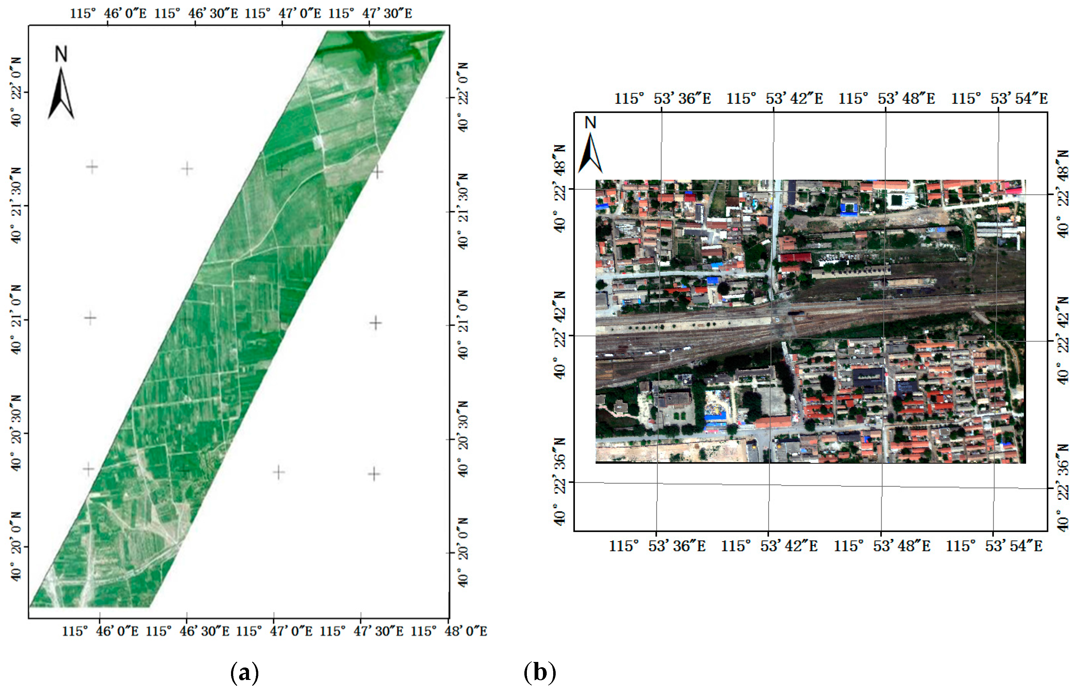
2. Study Area and Data Acquisition

2.1. Study Area

The test site was located in Huailai County, Zhangjiakou City, Hebei Province, China which is 10.3 km north–south and 17.5 km east–west with a total area of 180.25 km² (40°24′9.26′′–40°18′35.14′′N and 115°41′33.28′′–115°53′56.51′′E). In the site, two typical region were selected: one is farmland (Figure 1a) which comprises cropland, groves of pine and cypress trees, areas of shrubs, meadows, and wet lands, as well as standing water in a large reservoir. The other is a village which lies to the north of the station (Figure 1b). The village comprises many artificial structures, such as houses, roads, etc.

2.2. Airborne Data

Airborne CASI-1500 and SASI-600 data, together with in situ ground spectral measurements, were collected simultaneously at the Huailai test site from 11:00 to 13:00 on 21 July 2010.

The CASI and SASI instrument specifications are listed in

Table 1. Basic specifications of CASI and SASI.

Basic Specification	CASI-1500	SASI-600
Spectral range/(nm)	380–1050	950–2450
SPECTRAL SAMPLES	32 *	101
FWHM/(nm)	10.7	7.5
SIGNAL TO NOISE RATIO *	1095:1 peak	>1000
FIELD OF VIEW/°	40°	40°
IFOV/mrad	0.49	1.225
Pixels/Across-Track	1500 pixels	600 pixels
NOISE FLOOR	<2.0 DN	6.0 DN
Quantitative value/bit	14	14

FWHM, full width at half maximum; IFOV, instantaneous field-of-view. * CASI-1500 spectral samples are programmable, and there are 32 spectral samples in this study.

. Although the CASI-1500 can be programmed to collect in 288 spectral channels (<3.5 nm, full width at half maximum (FWHM) in the 380–1050-nm region), this study collected data in only 32 spectral channels (10.7 nm FWHM). SASI-600 has 101 channels in the 950–2450-nm region with a 15-nm sampling interval, and a 7.5-nm FWHM with a 40° field-of-view (FOV). CASI-1500 and SASI-600 can achieve spatial resolutions as high as 0.5 m and 1.2 m, respectively, when flown at altitudes of 1.0 km.

2.3. Field Measurement

In-situ surface reflectance spectra were measured with an ASD FieldSpec spectrometer (Analytical Spectral Devices Inc., Boulder, CO, USA) almost simultaneously to the CASI and SASI overflights (time differences were always no more than 30 min) from a nadir view while walking across the target. Spectralon™ was used for radiometric calibration to reflectance every half an hour. The ASD spectrometer has a 1-nm sample interval with a 3-nm spectral resolution in the VNIR range (350–1000 nm), and a 10-nm spectral resolution in the SWIR range (1001–2500 nm). We selected nine homogenous sample plots, which included maize (four plots), peanuts (one plot), soil (two plots), Chinese pine (one plot), and cement roads (one plot). For each plot, approximately 30 nadir-view spectra were collected for a surface area approximating the spatial resolution of CASI and SASI sensor data. These were then averaged to yield a representative reflectance spectrum for each plot.

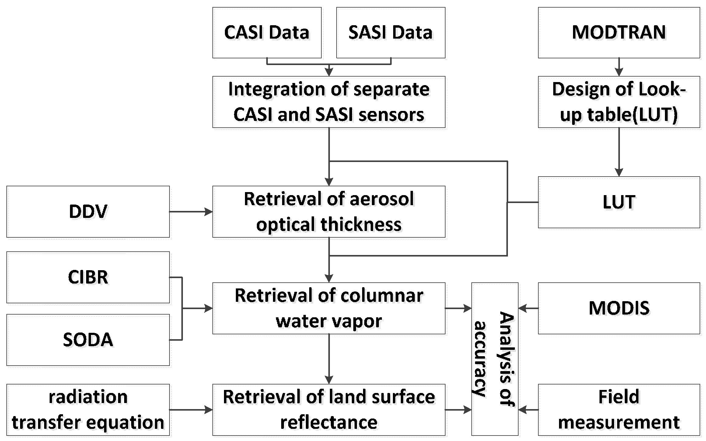
3. Methodology and Algorithm Employed

The methodology consisted of:

(1)

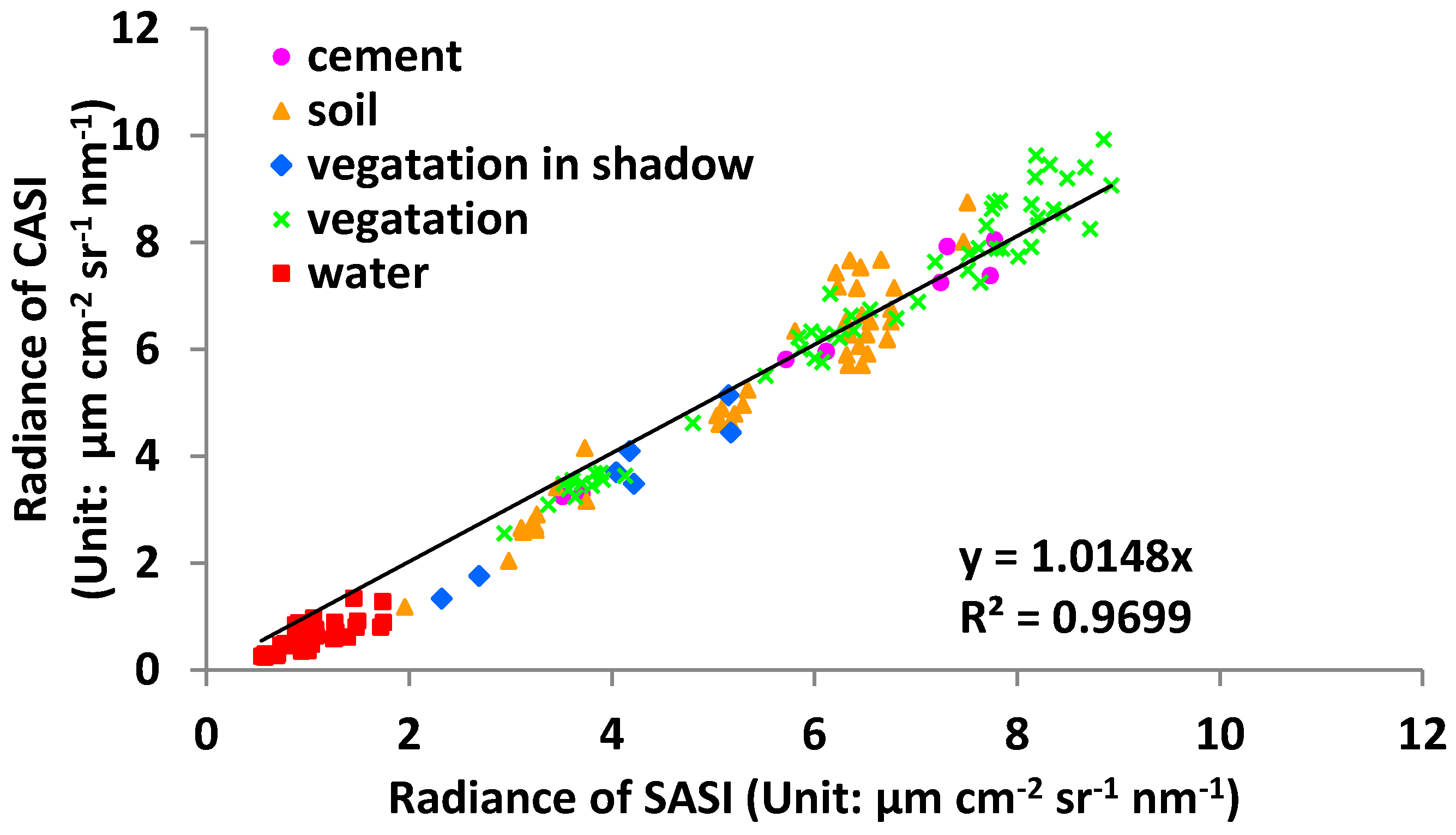
Radiometric and spatial cross-calibration of the CASI VNIR and SASI SWIR module data;

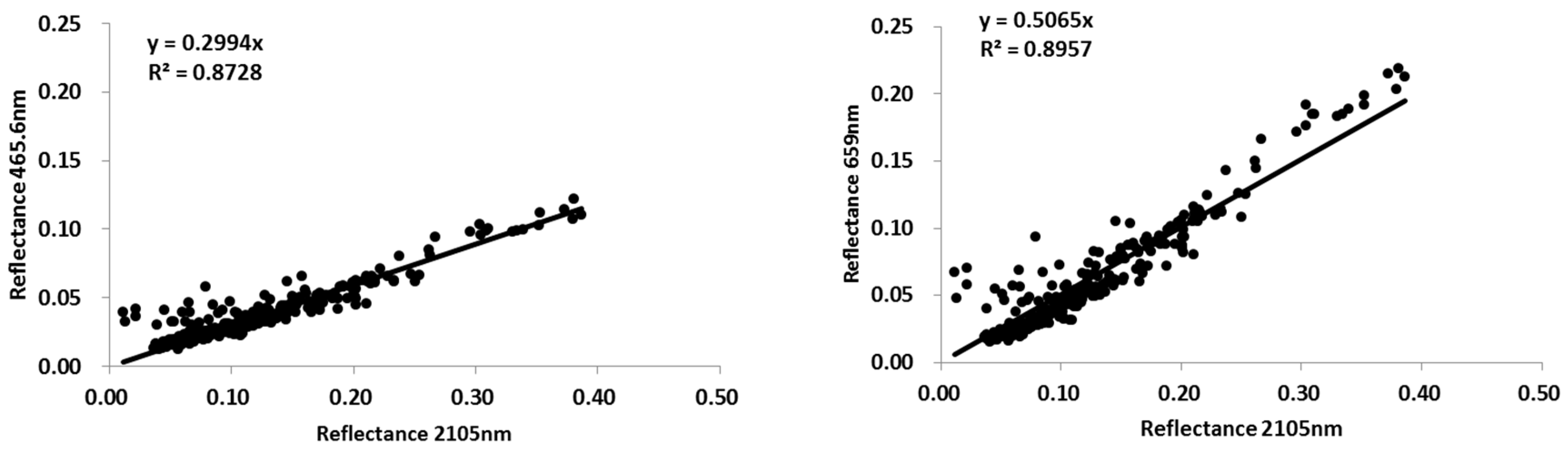
(2)

Establishing AOT@550 nm-related relationships between 465.6-nm/659-nm and 2105-nm wavelengths from the CASI and SASI data, and improving the minimization of the merit function;

(3)

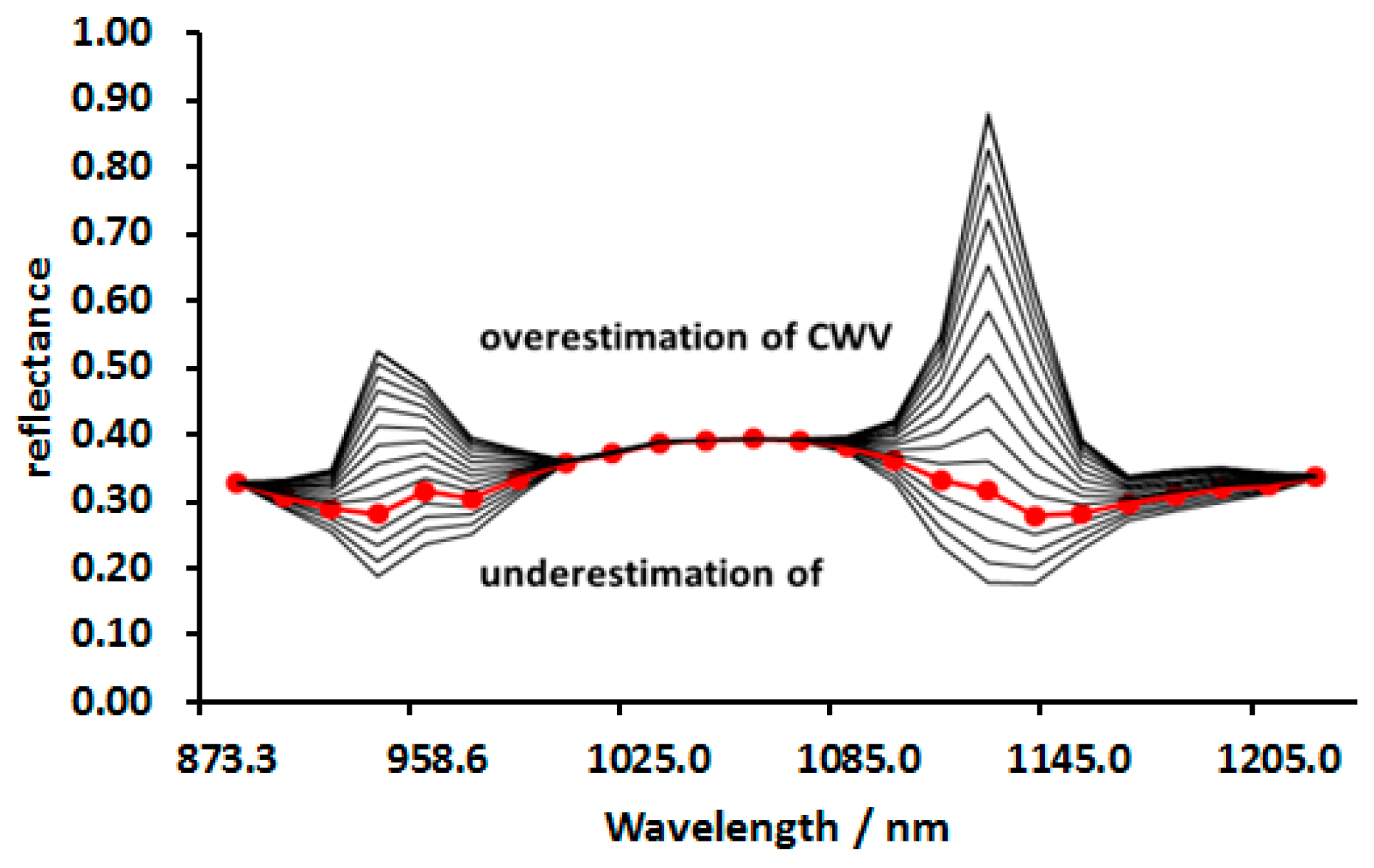
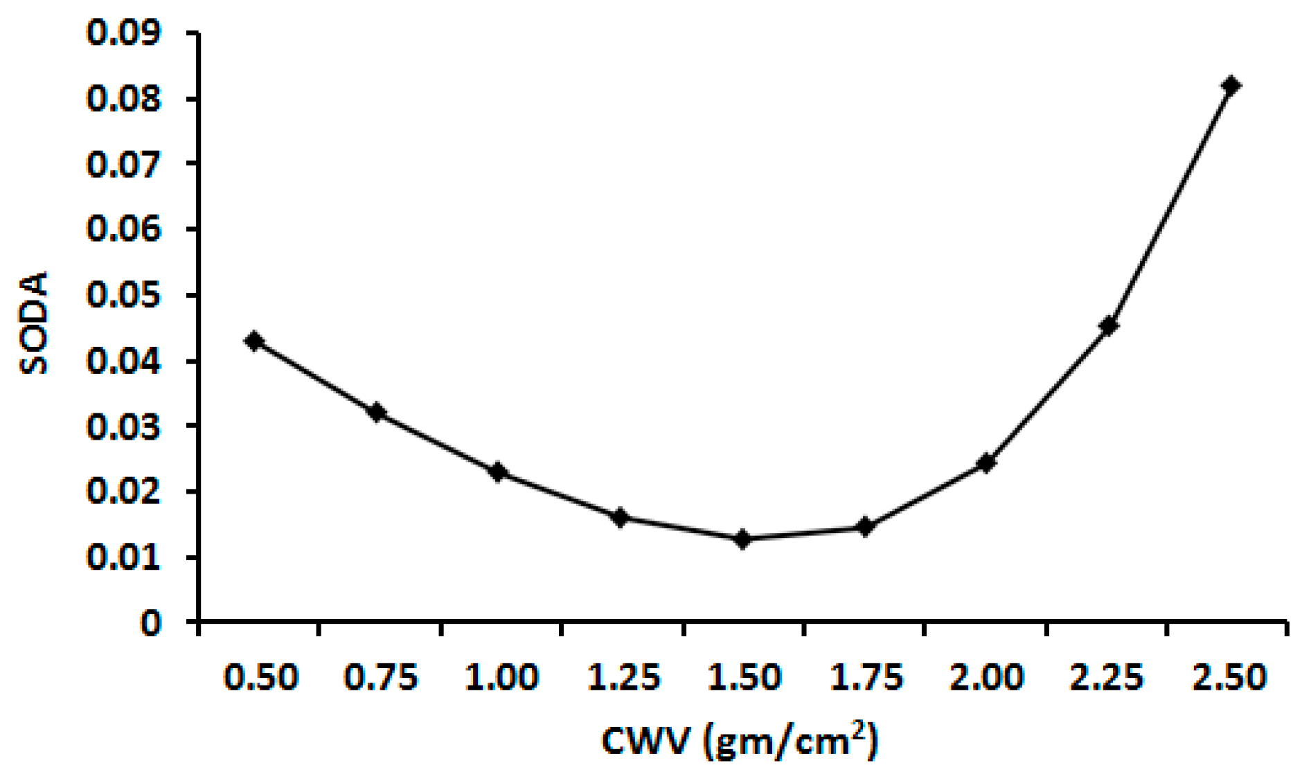
Estimating pixel-based CWV by initially using the CIBR method, and then by refining the CWV using SODA;

(4)

Applying Powell’s method to establish optimal pairing of AOT and CWV (Powell’s method is highly effective and robust for finding the optimal value); and

(5)

Validating the airborne results using the available ground-based reflectance data.

3.1. Integration of Separate CASI and SASI Sensors

CASI and SASI are independent sensors such that radiometric cross-calibration between them is essential if continuous VNIR–SWIR pixel spectra are to be generated, especially in the overlapping wavelength region of 950–1050 nm. The following details the process to integrate separate VNIR and SWIR modules from CASI and SASI instruments:

First, the radiance calibration method for CASI and SASI data were made based on the assumption of a linear sensor response function. The calibrated radiance (W∙sr⁻¹∙µm⁻¹∙m⁻²) for a given wavelength band is calculated by Equation (1)

$$L=c_1\times DN+c_2$$

(1)

where L is the calibrated radiance, DN is the raw instrument digital number, and c₁ and c₂ are the supplied calibration gains and offsets, respectively.

Next, the registration and geometry were corrected between the CASI and SASI images. The CASI 0.5-m pixel data were spatially resampled to SASI’s spatial resolution (1.2 m × 1.2 m) by picking 26 manually-selected ground control points (GCPs) and using a second-degree polynomial wrapping method with the nearest neighbor resampling method. For imaging spectrometry data, the nearest neighbor resampling method avoids spatial interpolation that leads to unmeasured, “unphysical” spectra [38,39]. The RMS registration error is <1 pixel.

Next, spectral bands in the overlapping region between the CASI and SASI modules were used to generate a single scaling coefficient to seamlessly join the integrated VNIR–SWIR pixel spectra. To achieve this, the SASI radiance spectra were down-sampled spectrally and spatially to the CASI resolution. This resulted in five overlapping bands, two of which showed poor signal-to-noise and were subsequently omitted. This left only three bands as residuals: 958.6 nm, 979.9 nm, and 1001.1 nm. These were then compared with 150 data points for both modules using linear regression analysis. The surface types included water, vegetation, soil, cement, and vegetation in shadow. The results (Figure 2) show that all three bands plot over the same regression line,

y = 1.0148x (R ² = 0.9699)

(2)

where x is the radiance of the SASI spectra and y is the radiance of the CASI spectra. The regression Equation (2) was then applied to the SASI data, and the CASI 380–969-nm bands were layered with the SASI 980–2450-nm bands. The RMSE between the two calibrations before applying the regression is 0.31 μmµcm⁻²µsr⁻¹µnm⁻¹ and 0.27 μmµcm⁻²µsr⁻¹µnm⁻¹ after applying the regression. The error was on the order of a few percent (Figure 2), which may be due to differences in the spectra response functions between the two modules.

3.2. Theoretical Background of Atmospheric Correction

It is necessary to give a brief description of the basic theoretical background of AC. Assuming Lambertian atmospheric scattering and surface reflectance, the at-sensor radiance at wavelengths 380–2500 nm are given in MODTRAN4 [8,26,40], which can be rewritten as:

$$L_{sensor,j}({\theta }_s,{\theta }_v,{\varphi }_s-{\varphi }_v)=L_{path,j}({\theta }_s,{\theta }_v,{\varphi }_s-{\varphi }_v)+\frac{T_{\uparrow }[(E_{dir}{\mu }_s+E_{dif}){\rho }_s]}{\pi (1-\mathrm{S}{\rho }_s)}$$

(3)

where $j$ is the $j\mathrm{th}$ band for the airborne sensor, ${\theta }_s$ is solar zenith angle, ${\theta }_v$ is sensor’s zenith angle, ${\varphi }_s-{\varphi }_v$ is azimuth angle between solar and sensor, ${\mu }_s$ is the cosine of the solar zenith angle (${\theta }_s$), $L_{sensor,j}$ is the Top-Of-Atmosphere (TOA) radiance measured by the sensor, $L_{path,j}$ is the atmospheric path radiance, $E_{dir}$ and $E_{dif}$ are the direct and diffuse fluxes arriving at ground level, respectively, ${\rho }_s$ is the surface reflectance, $s$ is the atmospheric spherical albedo accounting for multiple scattering between the atmosphere and the surface, and $T_{\uparrow }$ is the total atmospheric spectral transmittances for direct and diffuse radiance, which can be written as $T_{\uparrow }=T_{dif}^{\uparrow }+T_{dir}^{\uparrow }$.

From Equation (3), surface reflectance ${\rho }_s$ can be written as:

$${\rho }_s=\frac{A}{1+AS}$$

(4)

where

$$A=\frac{\pi \left(L_{sensor,j}({\theta }_s,{\theta }_v,{\varphi }_s-{\varphi }_v)-L_{path,j}({\theta }_s,{\theta }_v,{\varphi }_s-{\varphi }_v)\right)}{T_{\uparrow }[(E_{dir}{\mu }_s+E_{dif})}$$

(5)

Therefore, the atmospheric parameters, $S$, $L_{path,j}({\theta }_s,{\theta }_v,{\varphi }_s-{\varphi }_v)$, $T_{\uparrow }$, $E_{dir}$, ${\mu }_s$, and $E_{dif}$ are required prior to surface reflectance retrieval. It is a complex task to estimate these parameters because the radiative transfer formulas include many integro-differential functions that have no analytical solutions. Moreover, six atmospheric parameters are not included in the standard MODTRAN4 output, and have to be computed separately. The parameter $T_{dir}^{\uparrow }$ is an output of MODTRAN4. The parameters $E_{dir}$, $E_{dif}$, and ${\mu }_s$, can be calculated conveniently using the outputs of MODTRAN4. MODTRAN allows calculation of the atmospheric parameters $S$, $L_{path,j}({\theta }_s,{\theta }_v,{\varphi }_s-{\varphi }_v)$, and $T_{dif}^{\uparrow }$ using a 2-run surface reflectance scheme [7,8]. We tested this procedure for surface albedos of 0.15 and 0.5. The MODTRAN pack is accurate, but it is computationally very expensive and infeasible for handling large volume data sets. An alternative is to design off-line look-up table for certain input values.

3.3. Design of the Look-Up Table

To save on computation time, a LUT of atmospheric parameters was generated. Generally, six free parameters are used as input for the LUT: view zenith angle (VZA), solar zenith angle (SZA), relative azimuth angle (RAA), surface elevation (ELEV), AOT, which is related to visibility (VIS) by the Koschmieder Equation [8], and CWV. This study used nadir viewing, so VZA = 0°. Therefore, there are five free parameters in this framework.

Table 2. the breakpoint location of the LUT.

No.	SZA (°)	RAA (°)	ELEV (km)	AOT	CWV (gm/cm2)
1	0	0	0	0.05	0.50
2	10	25	0.7	0.10	0.75
3	20	50	1.5	0.15	1.00
4	30	75	2.5	0.20	1.25
5	40	100		0.25	1.50
6	50	125		0.30	1.75
7	60	150		0.35	2.00
8		180		0.45	2.25
9				0.50	2.50
10				0.55	2.75
11				0.60	3.00
12				0.65	3.25
13				0.70	3.50
14				0.80	3.75
15					4.00

SZA, solar zenith angle; RAA, relative azimuth angle; ELEV, surface elevation; AOT, aerosol optical thickness; CWV, columnar water vapor.

presents the LUT breakpoint location. The LUT items included 7 × 8 × 4 × 14 × 15 = 47,040 breakpoints, while the sextuplet of $\{$$S$, $L_{path,j}({\theta }_s,{\theta }_v,{\varphi }_s-{\varphi }_v)$, $T_{\uparrow }$, $E_{dir}$, ${\mu }_s$, and $E_{dif}$$\}$ for every breakpoint was stored in the LUT (Table 2). The LUT is stored as binary data, which can both reduce disk storage space and achieve fast LUT data random read [41]. The other main parameters are listed as follows:

(1)

Model Atmosphere Selection: Mid-Latitude Summer (45° North Latitude); atmospheric path is slant path; CO₂ mixing ratio is 360.0 ppmv; multiple scattering parameter is Distort and number of Distort stream equals to 8; the temperature at first boundary is based on the atmospheric temperature observed simultaneously at near-surface.

(2)

Aerosol and Cloud Option: Aerosol model is set to RURAL extinction, default VIS = 5 km; seasonal aerosol profile (ISEASN) is set to SPRING-SUMMER; the wind speed is set to the value measured simultaneously at near-surface; the weather is fine, and there is no cloud or rain.

(3)

Flight height = 1 km.

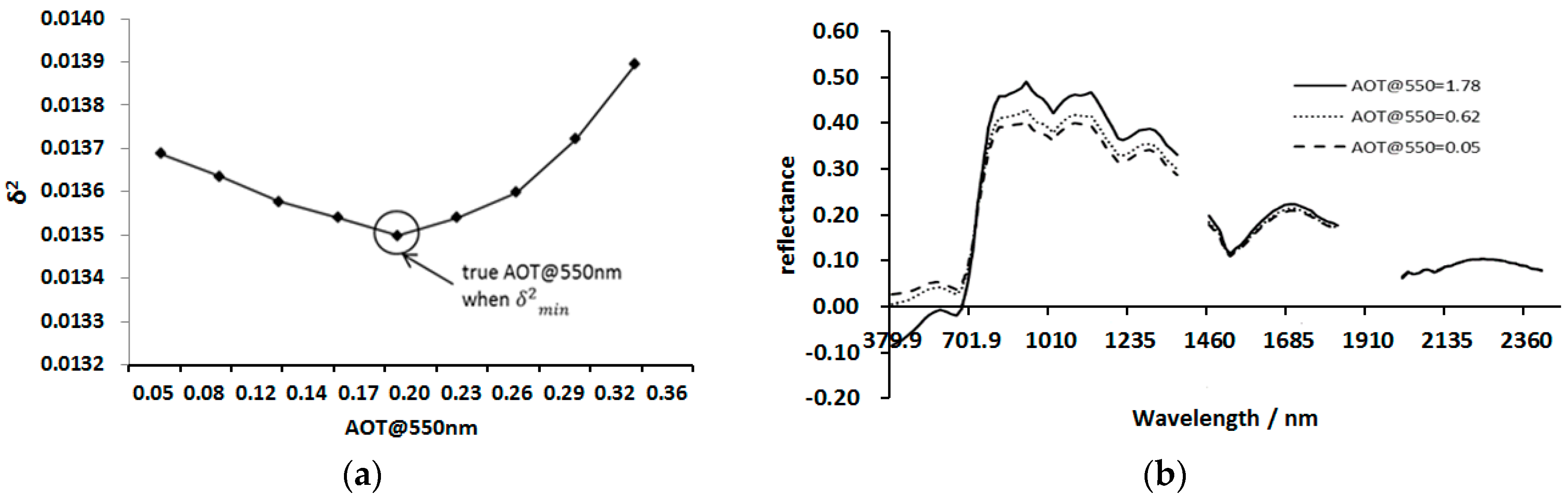
3.4. Retrieval of Aerosol Optical Thickness

The retrieval of AOT was based on the assumption that the AOT is spatially homogeneous across the study area. A rural aerosol model was also set in advance. DDV [11] was identified as a suitable reference to estimate the AOT over land surfaces. The method makes use of three channels to retrieve AOT@550 nm. In this study, we used the bands closest to those used by Kaufman et al. [11]. Specifically, we used bands centered at 465.6 nm, 659 nm, and 2105 nm to generate an empirical relationship automatically.

The first step of the automatic procedure to derive AOT was to select dark pixels in the blue (465.6 nm) and red (659 nm) channels using the SWIR channel (2105 nm). Image masks were used to ensure that pixels comprising water, snow, or ice, or that were contaminated by clouds, were not included in the derivation. A reflectance threshold between 0.01 and 0.25 was applied to the 2105-nm SWIR channel for the unmasked pixels, which produced another mask that was applied to the 659-nm reflectance channel. The masked areas were then sorted. Finally, the pixels with the brightest 50% and darkest 20% reflectances at 659 nm were removed to eliminate cloud and surface contamination further [22,24].

The second step was to estimate the reflectance ${\rho }_{p,465}^{meas}$ at 465.6 nm and ${\rho }_{p,659}^{meas}$ at 659 nm from the reflectance ${\rho }_{p,2105}$ at 2105 nm. The rationale for this step is to produce new empirical relationships between 465.6 nm/659 nm and 2105 nm for CASI and SASI sensors. Figure 3 shows the relationship between the 2105-nm and 659-nm surface reflectance (left) and the 2105-nm and 465.6-nm surface reflectance (right) based on 299 vegetation reflectance spectra that were measured with an ASD FieldSpec spectrometer and resampled according to the CASI and SASI band settings.

$${\rho }_{p,465}^{meas}=0.2994{\rho }_{p,2105},{\rho }_{p,659}^{meas}=0.5065{\rho }_{p,2105}$$

(6)

For comparison, Kaufman et al. found similar empirical relationships [11]:

$${\rho }_{470}=0.25{\rho }_{2130},{\rho }_{660}=0.50{\rho }_{2130}$$

(7)

Equation (6) and (7) indicate that the coefficient between the red and NIR bands was more stable than that between the blue and NIR bands. These results are similar to those of Levy [24].

The next step was to derive the AOT from the imagery. Aerosol scattering may have a significant effect on the water vapor absorption region (Figure 4b), while water vapor absorption has no significant impact on aerosol scattering [21,42,43]. Thus, AOT is accurate when the CWV is set to the default value in MODTRAN. For the study region, the parameters SZA, RAA, and ELEV were considered constant and known. Using the LUT, the atmospheric parameters were interpolated for certain AOTs@550 nm, and then the surface reflectance ${\rho }_{p,i}^{meas}$ was calculated from Equation (4). To achieve optimal AOT@550 nm, the retrieval was performed by minimizing the merit function:

$${\delta }^2=\frac{1}{n}{{\displaystyle \sum _{p=1}^n{\displaystyle \sum _{{\lambda }_i}^{chn}\frac{1}{{\lambda }_i^2}\left[{\rho }_{p,i}^{meas}-{\rho }_{p,i}^{sim}\right]}}}^2$$

(8)

where ${\rho }_{p,i}^{sim}$ is the surface reflectance simulated with the MODTRAN code and convolved according to the spectral response function of the ith channel; ${\lambda }_i$ is the center wavelength of the ith channel and $chn$ is the number of channels; $p$ is pixels; n is the number of pixels retrieved for the AOT estimation; and ${\rho }_{p,i}^{meas}$ is the surface reflectance computed using the DDV algorithm.

Figure 4a shows the cost function ${\delta }^2$ values of the AOT retrieval. ${\delta }^2<{\delta }_{\min }^2$ indicates cases where there was insufficient AOT for AC, and ${\delta }^2>{\delta }_{\min }^2$ indicates cases where there was too much AOT for AC. The point at which the minimum ${\delta }^2$ occurs represents the best estimate of AOT. Figure 4b shows the CASI and SASI reflectances over DDV in the presence of different AOTs. We found that surface reflectance decreases with increasing AOT@550 nm and may be negative if AOT@550 nm is overestimated.

3.5. Retrieval of Columnar Water Vapor

Atmospheric transmission features contain more high frequency components than surface ones. Therefore, the best water vapor estimation yields the smoothest retrieved surface reflectance in the water vapor absorbing regions, while inaccurate estimations of water vapor lead to residual high frequency peaks or troughs in the atmospheric absorption bands [21,44,45,46]. The degree of smoothness of individual reflectance curves can be used to interactively adjust for CWV. The measures of smoothness include variance and first- and second-order reflectance difference. This paper used SODA [18], which was written as:

$$SOD{A}_{H_{2}O}={\displaystyle \sum }_{\lambda =i}^N{\left({\rho }_{i-1}-2{\rho }_i+{\rho }_{i+1}\right)}^2$$

(9)

where N is the band number of the sensor from 890 nm to 1200 nm and $i=2,3,\dots N-1$.

The Powell method was applied to find the minimum $SOD{A}_{H_{2}O}$ with respect to the unknown CWV. This method has been widely used to find the local minimum of a function and requires initialization of CWV. For this purpose, the initial value of CWV was estimated using the CIBR method. The CWV error tolerance was set to 0.01 gm/cm². Figure 5 shows atmospheric line features in the upper and lower curves. The reflectance spectrum labeled with closed circles shows the smoothest spectrum, the uppermost spectrum is where CWV was overestimated, and the lowermost spectrum is where CWV was underestimated. Figure 6 shows $SOD{A}_{H_{2}O}$ smoothness measurements for various CWV values. The CWV value at the minimum $SOD{A}_{H_{2}O}$ value represents the best estimate of CWV.

3.6. Retrieval of Land Surface Reflectance

The final objective of this paper was to retrieve the land surface reflectance in the 380–2450-nm wavelength range. Once the AOT and CWV were estimated from hyperspectral images, the retrieval of surface reflectance was straightforward using at-sensor radiance images. For per-pixel reflectances, the process includes two steps. First, a general LUT must be interpolated. For certain pixels, the point to be interpolated represents the input of five atmospheric parameters $\{$SZA, RAA, ELEV, AOT, CWV$\}$, which were obtained from the above processes. The multidimensional Lagrange interpolation method was used to calculate the atmospheric parameters $\{$$S$, $L_{path,j}({\theta }_s,{\theta }_v,{\varphi }_s-{\varphi }_v)$, $T_{\uparrow }$, $E_{dir}$, ${\mu }_s$, and $E_{dif}$$\}$ in the 380–2450-nm wavelength range from the LUT. Next, the surface reflectance spectra are calculated using Equations (4) and (5). The most important steps, and a flow chart for this algorithm, are shown in Figure 7.

4. Results and Analysis

The validations of CASI and SASI AC and surface reflectance retrievals presented herein are given in two sections: analysis of atmospheric parameters retrievals and analysis of surface reflectance accuracy. The AOT was assumed to be homogeneous in this study area. Therefore, we discussed the accuracy of CWV and surface reflectance but not AOT.

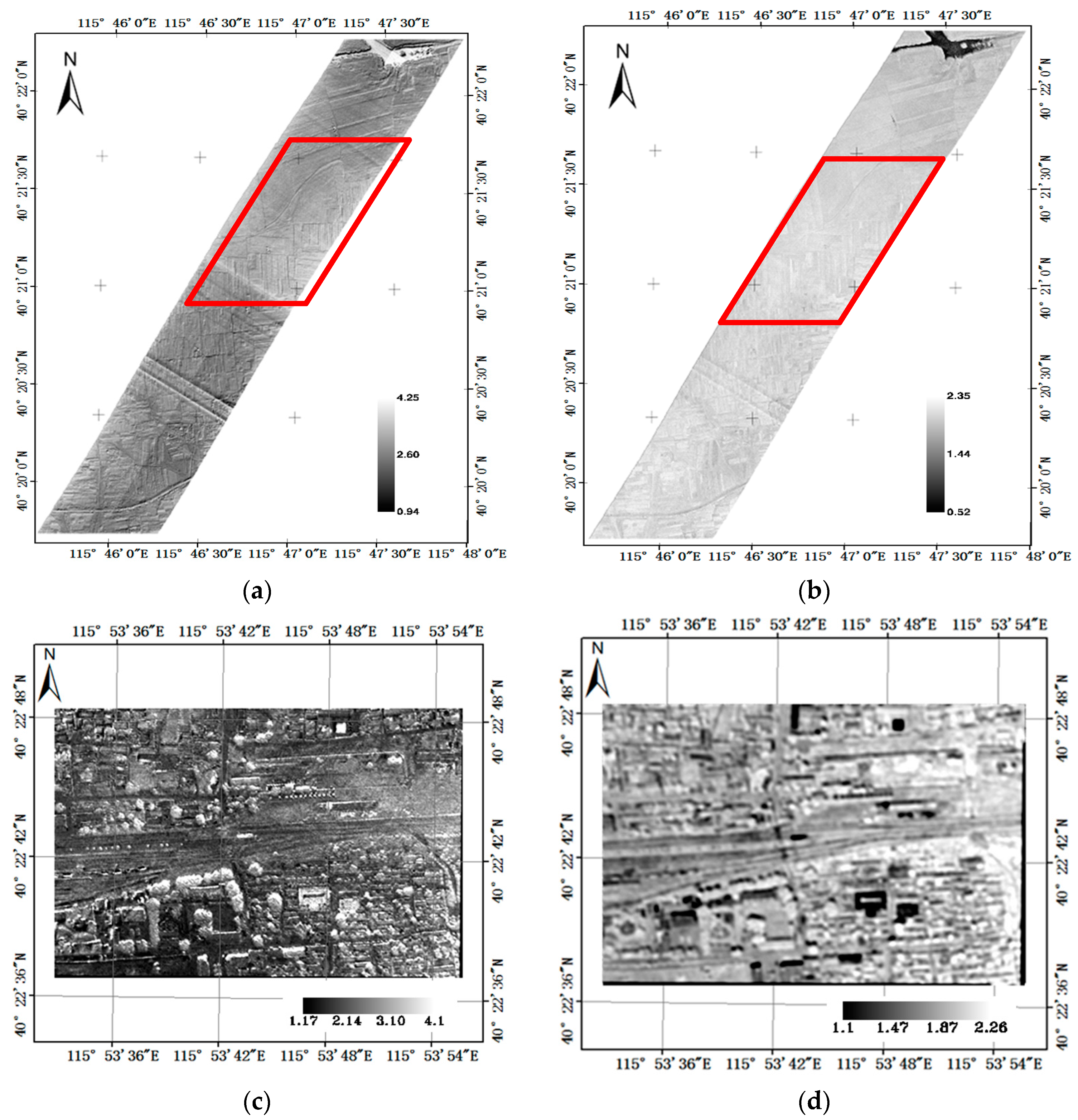
4.1. Analysis of CWV Accuracy

The CWV images from the CIBR and SODA methods are presented in Figure 8. The statistical results show that the CWV ranges of CIBR and SODA for farmland are 0.941–4.250 gm/cm² and 0.525–2.350 gm/cm², respectively, and the mean CWVs for CIBR and SODA are 2.222 ± 0.190 gm/cm² and 1.630 ± 0.111 gm/cm², respectively. For village, CWV ranges of CIBR and SODA are 1.167–4.067 gm/cm² and 1.08–2.261 gm/cm², respectively, and the mean CWVs for CIBR and SODA are 2.64 ± 0.174 gm/cm² and 1.963 ± 0.0934 gm/cm², respectively. The CIBR method estimates CWV with linear interpolation between two adjacent continuum values and assumes that reflectance is a linear function of wavelength. In fact, there was rain from 14 July to 20 July 2010, followed by clear and sunny conditions on 21 July 2010 when the field study was conducted. Therefore, the water contents of vegetation and soil are assumed to be high, which likely influenced the linearity of the surface reflectance around the water vapor absorption bands (Figure 9a). These changes could be introduced in the CWV retrieval [35]. Instead, we assessed accuracy qualitatively using the degree to which surface the features were subdued (ideally not apparent). In Figure 8a,b, there is obvious boundary characteristics in images from CIBR, while fuzzy boundary characteristics from SODA. In Figure 8c,d, it is easy to identify the canopy characteristics in images from CIBR, while difficult in images from SODA. Moreover, the standard deviation of images from SODA is less than that from CIBR. To this end, the SODA method showed fewer surface features compared with the CIBR method. These results are similar to those of Rodger [18].

Unfortunately, field CWV measurements were not collected with the airborne data simultaneously, so it is not possible to compare the accuracies of these methods. An alternate method is to validate the accuracy using MOD05 products, which are MODIS total precipitable water vapor (

Table 3. Comparison of CWV between CASI and SASI and MOD05 (unit: gm/cm²).

	MOD05	CIBR	SODA
1	3.233626	2.240634	1.563913
2	3.267766	2.410114	1.638526
3	3.267029	2.366965	1.643027
4	3.249835	2.279332	1.630543
R2 with MOD05		0.9152	0.8409

CIBR, Continuum Interpolated Band Ratio; SODA, second-order difference algorithm.

). The R² values between MOD05 and CIBR, and between MOD05 and SODA, were 0.9152 and 0.8409, respectively. There are significant relationships between them but there were significant differences between them (Table 3). The CWV from MOD05 is highest because MOD05 is total precipitable water vapor from the whole atmosphere, whereas CWVs from CASI and SASI are from 1 km above the surface.

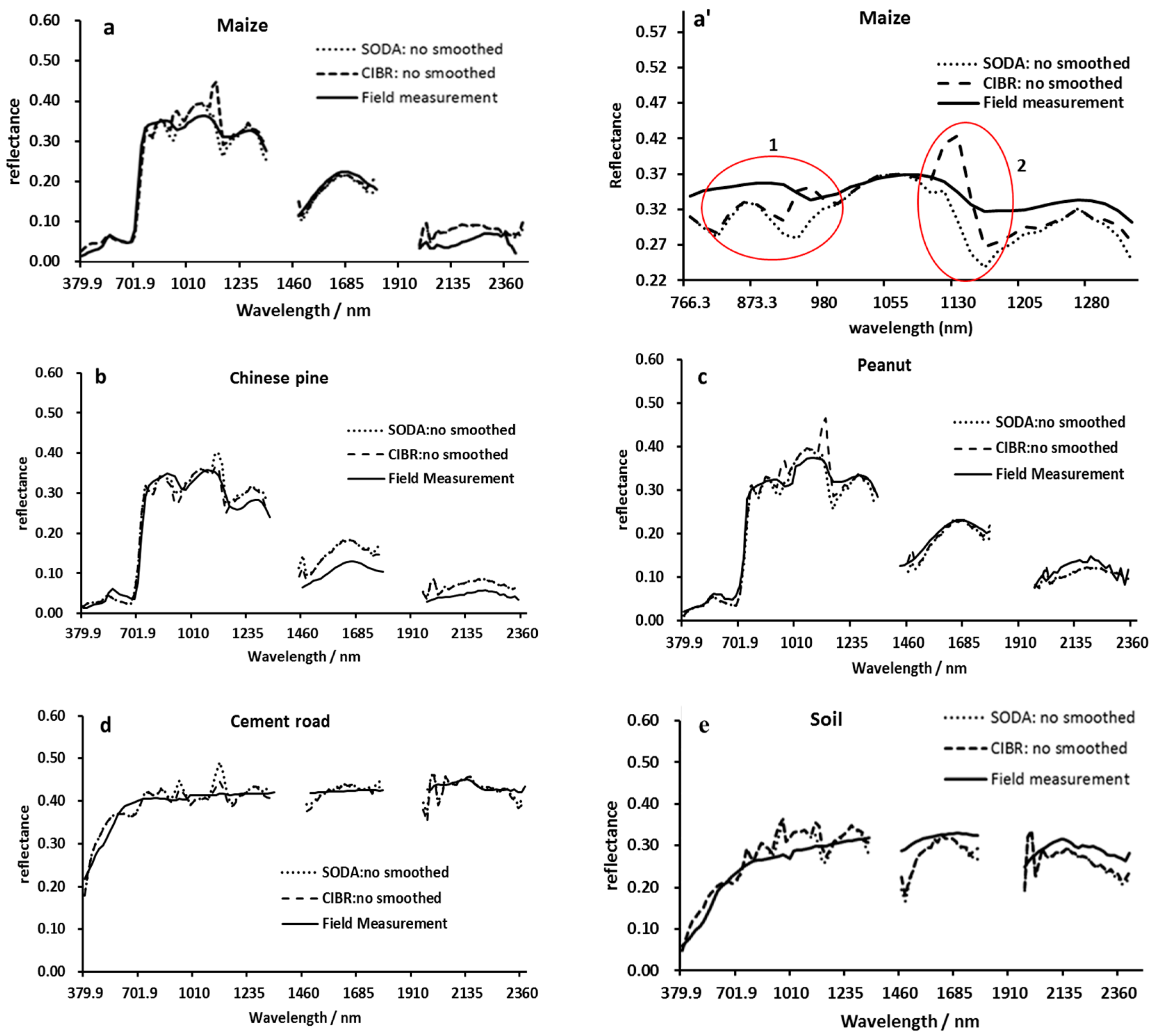
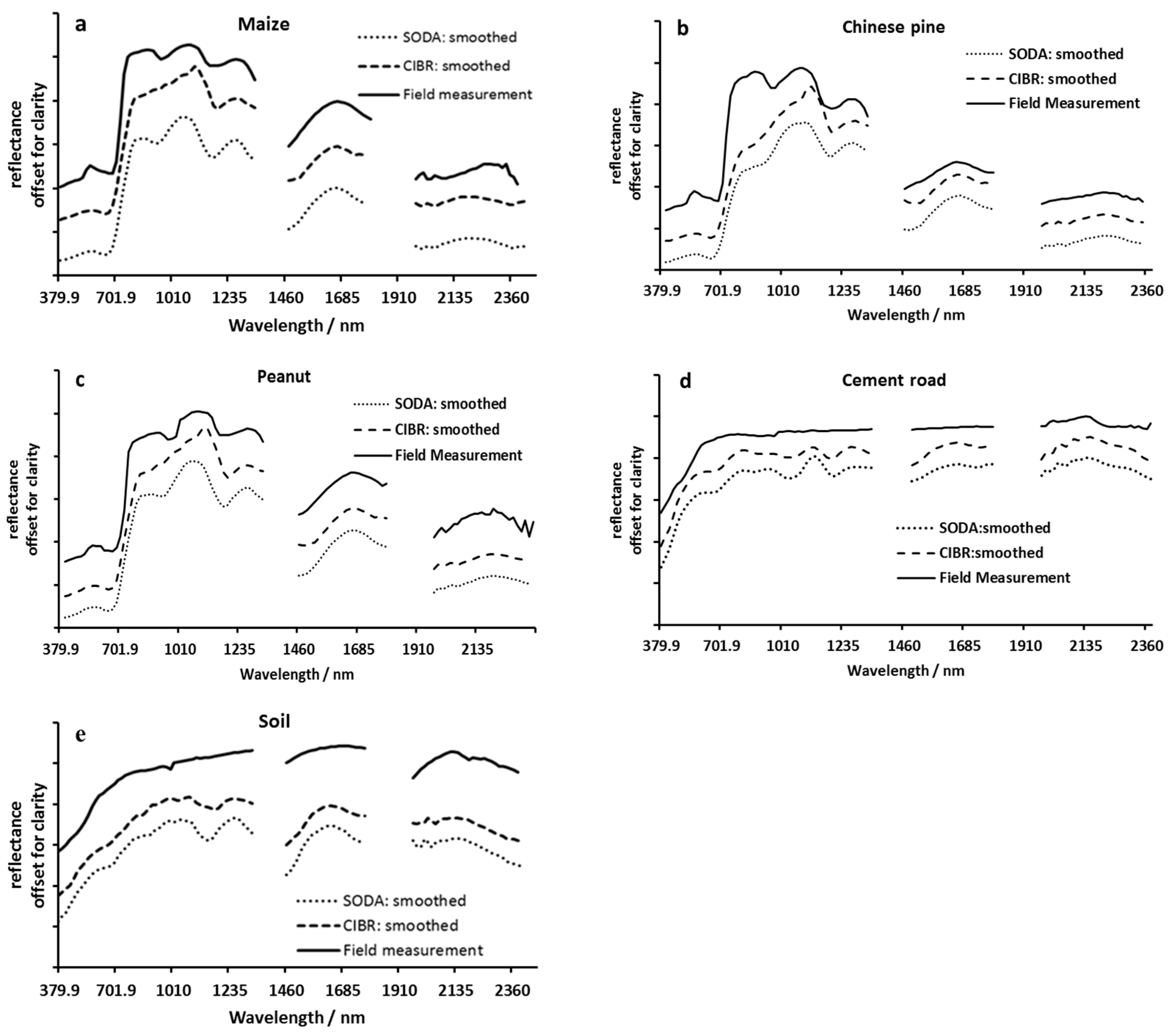
4.2. Analysis of Surface Reflectance Accuracy

The surface reflectance retrieval accuracy was assessed using five regions of interest from the fully processed images, green vegetation (maize, Chinese pine and peanut), cement road and bare soil, which were compared with ground ASD spectra from the same sites in Figure 9a–e, respectively. These show that outside of the major water vapor absorption bands (e.g., at ~940 and 1140 nm), the combined airborne CASI_SASI pixel surface reflectance spectra generated using both the CIBR and SODA methods closely matched the ground ASD spectra. However, the airborne SWIR results appear to have less contrast at increasing wavelengths. The main differences are in the 916–980-nm and 1110–1160-nm absorption regions, which may be caused by the overlap in spectral regions between CASI and SASI, because any errors in the cross calibration between the two sensors propagates down the algorithm. The derived remote sensing surface reflectance correlated significantly with ground spectra of comparable vegetation (R², 0.942 for maize; 0.972 for peanut; and 0.893 for Chinese pine), cement road (R², 0.832) and soil targets (R², 0.786). The RMSE of Chinese pine reflectance (RMSE, 0.0411) was the highest. The main cause may be the bidirectional reflectance distribution of canopy. The RMSE of soil reflectance (RMSE, 0.0356) was somewhat higher than that of vegetation except Chinese pine. A possible cause of the ASD and retrieved reflectance may be a combination of surface roughness and non-Lambertian and directional effects of the soil surface [21]. These factors can affect both the at-sensor and ground-based data. Additionally, a prominent red edge of vegetation is clearly seen around 700 nm in Figure 9e due to the adjacency effect. However, both the spectral shape and RMSE suggest that the method proposed in this paper may be reliable enough for in-scene AC and surface reflectance retrieval from hyperspectral remote sensing data.

Within the major water vapor absorption region at 940, 1140, 1400 and 1900 nm, there were apparent differences among the ROI spectra. That is, the green vegetation airborne and field spectra are in close agreement for all but the 940-nm water band. The airborne bare soil spectra appear to undercompensate for water vapor at 1140 nm and 1400 nm, but less so for the 940- and 1900-nm features using both the CIBR and SODA methods. Rodger found a similar result and suggested that the HITRAN database may require updating [18]. To highlight the differences between the CIBR and SODA methods, surface reflectance of maize within 766–1340 nm are scaled in Figure 9a’. The differences occurred at 937.3-nm, 1130-nm and their vicinity bands because the 937.3-nm band and its vicinity bands are used in the CIBR method, while bands from 890–1200 nm are used in the SODA method. On the other hand, the reflectance spectra at the 958.5-nm and 1130-nm bands had significant spikes, which indicates that the CWV was overestimated based on the analyses shown in Figure 5. Conversely, it would appear that the SODA underestimated the CWV.

To construct the final spectra, smoothing techniques are sometimes used to remove the remaining atmospheric residuals [47,48,49]. To evaluate this, a moving average filter with five bands was applied to the spectra (Figure 10). The five panels show that the filter removed some small spikes. The smoothed spectra appears to be improved, although

Table 4. Comparison of R² and RMSE between the retrieved surface reflectance from airborne images and at-ground reflectance.

Surface Type		R2	RMSE
Maize	not smoothed	0.945	0.0252
Maize	smoothed	0.974	0.0247
Peanut	not smoothed	0.972	0.0192
Peanut	smoothed	0.982	0.0177
Chinese pine	not smoothed	0.893	0.0411
Chinese pine	smoothed	0.895	0.0404
Cement road	not smoothed	0.832	0.0211
Cement road	smoothed	0.908	0.0141
Soil	not smoothed	0.786	0.0356
Soil	smoothed	0.801	0.0317

shows that there were no significant improvements in R² or RMSE between the retrieved surface reflectances from airborne images and at-ground reflectances. However, care must be taken when using this approach as smoothing can alter the diagnostic absorption features. This is especially relevant for materials such as minerals.

5. Conclusions

Recently, airborne hyperspectral data across VNIR–SWIR have become more commercially available. However, in applications where the completed VNIR–SWIR regions are required, there is usually a need to integrate data from separate sensors. This study investigated some of the key issues that must be considered to provide accurate reflectance data from such integrated use. We propose radiometric and spatial cross-calibration, design of an LUT, and retrieval of AOT, CWV and surface reflectance to accomplish this. The LUT is built using the outputs of the MODTRAN-based atmospheric modeling code and has six parameters $\{$$S$, $L_{path,j}({\theta }_s,{\theta }_v,{\varphi }_s-{\varphi }_v)$, $T_{\uparrow }$, $E_{dir}$, ${\mu }_s$, and $E_{dif}$$\}$ for every breakpoint. To improve the accuracy of the AOT estimation, new empirical relationships between 465.6 nm/659 nm and 2105 nm are built according to the characteristics of the CASI and SASI sensors, and by minimizing the merit function to retrieve AOT@550 nm. For CWV retrieval, the SODA and CIBR methods were used. The results show that CIBR appeared, in this case, to overestimate CWV due to the presence of leaf water in the vegetation and possible water uptake in the soil. Conversely, the SODA results indicate that CWV was possibly underestimated. There may be several reasons for the over and underestimations. One is that a discrepancy still exists between the CASI and SASI sensor cross-calibration. Any error that exists after the cross-calibration of the two sensors propagates throughout the algorithm and may produce errors in the retrievals.

Using separate ACs to the two sensors may solve the aforementioned problem. However, this means that two separate water vapor regions must be used, 820-nm or 940- nm for the CASI, and 1140-nm for the SASI sensor. Consideration must also be made to cross check the water vapor values retrieved from the different regions. This line of research will be pursued in the next stage of this study.

The sensor cross-calibration issue of possible downstream effects on ACs emphasizes the importance of cross-calibration between the sensors when using them in an integrated manner. This is a difficult task radiometrically because the overlapping regions are at the edge of the detectors and inherently suffer from lower SNR. Furthermore, geometric calibrations of the sensors are also non-trivial for the particular data set. If the accuracy geographical coordinates information could be given, the geometric calibration is fairly straightforward using geographical coordinates information. However, Airborne hyperspectral sensors suffer from distortions because of the sensor movement during data acquisition and mechanically stabilizing platforms cannot remove these effects completely [38,39]. Therefore, it may be fruitful to focus on developing methods for this topic for future work since there are now many operational sensors that incorporate separate sensors.

Another reason for the discrepancies in the CWV estimations may be spectral miscalibration. We attempted to recalibrate the CASI and SASI sensors using known atmospheric features identified in each of the sensors but no significant improvements were observed. This may be attributed to the limited and broad bands, which may be insufficient to characterize the oxygen feature.

Spectral smoothing was tested to assess its utility in removing residual atmospheric features that were unaccounted for. Although smoothing does appear to “smooth” out the peaks and troughs, we demonstrated that it does not necessarily provide an accurate result. The experiment showed that smoothing removed and distorted diagnostic spectral features. This is especially important for narrow features such as those found in minerals.

It must be acknowledged that the DDV method is limited to vegetated areas and dark soils (excluding ice/snow cover and desert). Future work could include the development of a new method for AOT retrieval from hyperspectral data over bright, reflective regions. Additionally, the effects of elevation, adjacency, and direction on the surface were not adequately considered in this paper due to the study region primarily being topographically flat. The highest RMSE of Chinese pine reflectance is because of the bidirectional reflectance distribution of canopy, but it is difficult to find the adequate modeling of the surface directional reflectance which could be plugged into an operational procedure. Therefore, errors associated to the Lambertian approach are assumed to be intrinsic to the method. Certainly, these effects will be considered in future work that seeks to improve the proposed technique.

References

1. Goetz, A.F.H. Three decades of hyperspectral remote sensing of the Earth: A personal view. Remote Sens. Environ. 2009, 113, S5–S16. [Google Scholar] [CrossRef]
2. Tong, Q.; Xue, Y.; Zhang, L. Progress in hyperspectral remote sensing science and technology in China over the past three decades. IEEE J. Sel. Top. Appl. Earth Obs. Remote Sens. 2014, 7, 70–91. [Google Scholar] [CrossRef]
3. Farrand, W.H.; Singer, R.B.; Merényi, E. Retrieval of apparent surface reflectance from AVIRIS data: A comparison of empirical line, radiative transfer, and spectral mixture methods. Remote Sens. Environ. 1994, 47, 311–321. [Google Scholar] [CrossRef]
4. Kruse, F.A. Use of airborne imaging spectrometer data to map minerals associated with hydrothermally altered rocks in the northern Grapevine Mountains, Nevada, and California. Remote Sens. Environ. 1988, 24, 31–51. [Google Scholar] [CrossRef]
5. Goetz, A.F.; Srivastava, V. Mineralogical Mapping in the Cuprite Mining District, Nevada. Available online: https://ntrs.nasa.gov/search.jsp?R=19860002152 (accessed on 23 November 2016).
6. Vermote, E.F.; Tanre, D. Second simulation of the satellite signal in the solar spectrum, 6S: An overview. IEEE Trans. Geosci. Remote Sens. 1997, 35, 675–686. [Google Scholar] [CrossRef]
7. Guanter, L.; Richter, R.; Kaufmann, H. On the application of the MODTRAN4 atmospheric radiative transfer code to optical remote sensing. Int. J. Remote Sens. 2009, 30, 1407–1424. [Google Scholar] [CrossRef]
8. Berk, A. MODTRAN4 User’s Manual; Air Force Research Laboratory, Space Vehicles Directorate: Hanscom Air Force Base, MA, USA, 1999; pp. 1–5. [Google Scholar]
9. Sismanidis, P.; Karathanassi, V. Evaluation of atmospheric correction to airborne hyperspectral data relying on radiative transfer concepts. Int. J. Remote Sens. 2013, 34, 8566–8587. [Google Scholar] [CrossRef]
10. Gao, B.-C. Atmospheric correction algorithms for hyperspectral remote sensing data of land and ocean. Remote Sens. Environ. 2009, 113, S17–S24. [Google Scholar] [CrossRef]
11. Kaufman, Y.; Tanré, D.; Remer, L.A.; Vermote, E.F.; Chu, A.; Holben, B.N. Operational remote sensing of tropospheric aerosol over land from EOS moderate resolution imaging spectroradiometer. J. Geophys. Res. Atmos. 1997, 102, 17051–17067. [Google Scholar] [CrossRef]
12. Kaufman, Y.J. The MODIS 2.1-μm channel-correlation with visible reflectance for use in remote sensing of aerosol. IEEE Trans. Geosci. Remote Sens. 1997, 35, 1286–1298. [Google Scholar]
13. Schläpfer, D. Atmospheric Precorrected Differential Absorption Technique to Retrieve Columnar Water Vapor. Remote Sens. Environ. 1998, 65, 353–366. [Google Scholar] [CrossRef]
14. Bojinski, S. Aerosol mapping over land with imaging spectroscopy using spectral autocorrelation. Int. J. Remote Sens. 2004, 25, 5025–5047. [Google Scholar] [CrossRef]
15. Zhao, X.; Liang, S.L.; Liu, S.H.; Wang, J.D.; Qin, J.; Li, Q.; Li, X.W. Improvement of dark object method in atmospheric correction of hyperspectral remotely sensed data. Sci. China Ser. D Earth Sci. 2008, 51, 349–356. [Google Scholar] [CrossRef]
16. Gao, B.-C.; Kaufman, Y.J. Water vapor retrievals using Moderate Resolution Imaging Spectroradiometer (MODIS) near-infrared channels. J. Geophys. Res. 2003, 108, 4389. [Google Scholar] [CrossRef]
17. Guanter, L.; Alonso, L.; Moreno, J. A method for the surface reflectance retrieval from PROBA/CHRIS data over land: Application to ESA SPARC campaigns. IEEE Trans. Geosci. Remote Sens. 2005, 43, 2908–2917. [Google Scholar] [CrossRef]
18. Rodger, A. SODA: A new method of in-scene atmospheric water vapor estimation and post-flight spectral recalibration for hyperspectral sensors: Application to the HyMap sensor at two locations. Remote Sens. Environ. 2011, 115, 536–547. [Google Scholar] [CrossRef]
19. Gao, B.-C.; Goetz, A.F.H. Determination of total column water vapor in the atmosphere at high spatial resolution from AVIRIS data using spectral curve fitting and band ratioing techniques. Imaging Spectrosc. Terr. Environ. 1990, 1298. [Google Scholar] [CrossRef]
20. Gao, B.C.; Goetz, A.F. Column atmospheric water vapor and vegetation liquid water retrievals from airborne imaging spectrometer data. J. Geophys. Res. Atmos. 1990, 95, 3549–3564. [Google Scholar] [CrossRef]
21. Guanter, L.; Estellés, V.; Moreno, J. Spectral calibration and atmospheric correction of ultra-fine spectral and spatial resolution remote sensing data. Application to CASI-1500 data. Remote Sens. Environ. 2007, 109, 54–65. [Google Scholar] [CrossRef]
22. Remer, L.A. The MODIS aerosol algorithm, products, and validation. J. Atmos. Sci. 2005, 62, 947–973. [Google Scholar] [CrossRef]
23. Levy, R.C.; Remer, L.A.; Kaufman, Y.J. Effects of neglecting polarization on the MODIS aerosol retrieval over land. IEEE Trans. Geosci. Remote Sens. 2004, 42, 2576–2583. [Google Scholar] [CrossRef]
24. Levy, R.C.; Remer, L.A.; Mattoo, S.; Vermote, E.F.; Kaufman, Y.J. Second-generation operational algorithm: Retrieval of aerosol properties over land from inversion of Moderate Resolution Imaging Spectroradiometer spectral reflectance. J. Geophys. Res. Atmos. 2007, 112, D13211. [Google Scholar] [CrossRef]
25. Guanter, L. New Algorithms for Atmospheric Correction and Retrieval of Biophysical Parameters in Earth Observation: Application to ENVISAT/MERIS Data. Available online: http://roderic.uv.es/handle/10550/15793 (accessed on 23 November 2016).
26. Guanter, L.; Gómez-Chova, L.; Moreno, J. Coupled retrieval of aerosol optical thickness, columnar water vapor and surface reflectance maps from ENVISAT/MERIS data over land. Remote Sens. Environ. 2008, 112, 2898–2913. [Google Scholar] [CrossRef]
27. Hsu, N.C.; Tsay, S.-H.; King, M.D.; Herman, J.R. Aerosol properties over bright-reflecting source regions. IEEE Trans. Geosci Remote Sens. 2004, 42, 557–569. [Google Scholar] [CrossRef]
28. Hsu, N.C. Deep blue retrievals of Asian aerosol properties during ACE-Asia. IEEE Trans. Geosci. Remote Sens. 2006, 44, 3180–3195. [Google Scholar] [CrossRef]
29. Bassani, C.; Cavalli, R.M.; Pignatti, S. Aerosol optical retrieval and surface reflectance from airborne remote sensing data over land. Sensors 2010, 10, 6421–6438. [Google Scholar] [CrossRef] [PubMed]
30. Frouin, R.; Deschamps, P.-Y.; Lecomte, P. Determination from space of atmospheric total water vapor amounts by differential absorption near 940 nm: Theory and airborne verification. J. Appl. Meteorol. 1990, 29, 448–460. [Google Scholar] [CrossRef]
31. Green, R.; Carrere, V.; Conel, J. Measurement of atmospheric water vapor using the Airborne Visible/Infrared Imaging Spectrometer. In Proceedings of the Workshop Imaging Processing, Sparks, NV, USA, 23 May 1989.
32. Bruegge, C.J. In-situ atmospheric water-vapor retrieval in support of AVIRIS validation. Proc. SPIE 1990, 1298. [Google Scholar] [CrossRef]
33. Bruegge, C.J. Water vapor column abundance retrievals during FIFE. J. Geophys Res. Atmos. 1992, 97, 18759–18768. [Google Scholar] [CrossRef]
34. Schläpfer, D.; Keller, J.; Itten, K. Imaging Spectrometry of Tropospheric Ozone and Water Vapor; A.A. Balkema: Rotterdam, The Netherlands, 1996; pp. 439–446. [Google Scholar]
35. Carrère, V.; Conel, J.E. Recovery of atmospheric water vapor total column abundance from imaging spectrometer data around 940 nm—Sensitivity analysis and application to airborne visible/infrared imaging spectrometer (AVIRIS) data. Remote Sens. Environ. 1993, 44, 179–204. [Google Scholar] [CrossRef]
36. Hu, S. Integrated Retrieval technique for Surface Reflectance from Spaceborne Hyperspectral Data. Ph.D. Thesis, Chinese Academy of Sciences, Beijing, China, 2013. [Google Scholar]
37. Richter, R.; Schläpfer, D.; Müller, A. An automatic atmospheric correction algorithm for visible/NIR imagery. Int. J. Remote Sens. 2006, 27, 2077–2085. [Google Scholar] [CrossRef]
38. Schläpfer, D.; Richter, R. Geo-atmospheric processing of airborne imaging spectrometry data. Part 1: parametric orthorectification. Int. J. Remote Sens. 2002, 23, 2609–2630. [Google Scholar] [CrossRef]
39. Richter, R.; Schläpfer, D. Geo-atmospheric processing of airborne imaging spectrometry data. Part 2: atmospheric/topographic correction. Int. J. Remote Sens. 2002, 23, 2631–2649. [Google Scholar]
40. Richter, R. A fast atmospheric correction algorithm applied to Landsat TM images. Remote Sens. 1990, 11, 159–166. [Google Scholar] [CrossRef]
41. Hu, S.; She, X.; Tong, Q. Design and interpolation of a general look-up table for remote sensing image atmospheric correction. J. Remote Sens. 2014, 18, 45–60. [Google Scholar]
42. Chylek, P.; Borel, C.C.; Clodius, W.; Pope, P.A.; Rodger, A.P. Satellite-based columnar water vapor retrieval with the multi-spectral thermal imager (MTI). Geosci. IEEE Trans. Remote Sens. 2003, 41, 2767–2770. [Google Scholar] [CrossRef]
43. Bennartz, R.; Fischer, J. Retrieval of columnar water vapour over land from backscattered solar radiation using the Medium Resolution Imaging Spectrometer. Remote Sens. Environ. 2001, 78, 274–283. [Google Scholar] [CrossRef]
44. Qu, Z.; Kindel, B.C.; Goetz, A.F. The high accuracy atmospheric correction for hyperspectral data (HATCH) model. IEEE Trans. Geosci Remote Sens 2003, 41, 1223–1231. [Google Scholar]
45. Gao, B.-C.; Heidebrecht, K.B.; Goetz, A.F. Derivation of scaled surface reflectances from AVIRIS data. Remote Sens. Environ. 1993, 44, 165–178. [Google Scholar] [CrossRef]
46. Guanter, L.; Richter, R.; Moreno, J. Spectral calibration of hyperspectral imagery using atmospheric absorption features. Appl. Opt. 2006, 45, 2360–2370. [Google Scholar] [CrossRef] [PubMed]
47. Adler-Golden, S.M. Atmospheric correction for shortwave spectral imagery based on MODTRAN4. Proc. SPIE 1999, 3753, 61–69. [Google Scholar]
48. Gao, B.-C.; Liu, M.; Davis, C.O. A new and fast method for smoothing spectral imaging data. In Summaries of the Seventh JPL Airborne Earth Science Workshop; AVIRIS Workshop: Pasadena, CA, USA, 1998. [Google Scholar]
49. Joseph, B. Leveraging the high dimensionality of AVIRIS data for improved subQpixel target unmixing and rejection of false positives: mixure tuned matched filtering. In Summaries of the Seventh Annual JPL Airborne Geoscience Workshop; AVIRIS Workshop: Pasadena, CA, USA, 1998. [Google Scholar]
Figure 1. Map of the study area in Huailai County, Zhangjiakou City, Hebei Province, China: (a) the farmland; and (b) the village.
Remotesensing 09 00217 g001
Figure 2. Scatter diagram of the relationship between Compact Airborne Spectrographic Imager (CASI) and SWIR Airborne Spectrographic Imager (SASI) for the three selected overlapping bands for 10 different ROIs.
Remotesensing 09 00217 g002
Figure 3. Scatter diagrams between the 2105-nm and 465.6-nm/659-nm surface reflectances.
Remotesensing 09 00217 g003
Figure 4. (a) Cost function δ 2 values of the aerosol optical thickness (AOT) retrieval. The best estimates of AOT occur at the minimum. (b) CASI and SASI reflectances over Dense Dark Vegetation (DDV) in the presence of different AOTs.
Remotesensing 09 00217 g004
Figure 5. Second-order difference algorithm (SODA)-based reflectance spectra retrievals using different columnar water vapor values (CWVs) within the 890-nm and 1230-nm regions. The reflectance spectral labeled by closed circle “●” is the smoothest spectral, upper which means the overestimated CWV, and lower which means the under estimated CWV.
Remotesensing 09 00217 g005
Figure 6. S O D A H 2 O smoothness values of reflectance curve indices that are insensitive to CWV. The best estimate of CWV occurs at the minimum S O D A H 2 O value.
Remotesensing 09 00217 g006
Figure 7. Flow chart for land surface reflectance retrieval.
Remotesensing 09 00217 g007
Figure 8. The estimated CWVs using Continuum Interpolated Band Ratio (CIBR) and SODA methods: (a) farmland + CIBR; (b) farmland + SODA; (c) village + CIBR; and (d) village + SODA. For farmland, the mean CWVs using CIBR and SODA are 2.222 ± 0.190 gm/cm2 and 1.630 ± 0.111 gm/cm2, respectively. For village, the mean CWVs using CIBR and SODA are 2.64 ± 0.174 gm/cm2 and 1.963 ± 0.0934 gm/cm2, respectively.
Remotesensing 09 00217 g008
Figure 9. Comparison of the surface reflectance from retrieved airborne images with the at-ground reflectance. (a) Maize, (b) Chinese pine, (c) Peanut, (d) Cement road, and (e) Soil. Symbol SODA is the second-order difference algorithm to retrieve columnar water vapor and CIBR is Continuum Interpolated Band Ratio algorithm to retrieve columnar water vapor. Symbol “no smoothed” is that the surface reflectance spectra are calculated using Equations (4) and (5) without smoothing techniques. To highlight the differences between the CIBR and SODA methods, surface reflectance of maize within 766–1340 nm are scaled in panel (a’).
Remotesensing 09 00217 g009
Figure 10. Spectra from Figure 9a,b smoothed with a moving average and offset. (a) Maize, (b) Chinese pine, (c) Peanut, (d) Cement road, and (e) Soil. Symbol SODA is the second-order difference algorithm to retrieve columnar water vapor and CIBR is Continuum Interpolated Band Ratio algorithm to retrieve columnar water vapor. Symbol “smoothed” is that the surface reflectance spectra are calculated using smoothing techniques.
Remotesensing 09 00217 g010