Calibration and Validation of a Detailed Architectural Canopy Model Reconstruction for the Simulation of Synthetic Hemispherical Images and Airborne LiDAR Data

Abstract

Canopy density measures such as the Leaf Area Index (LAI) have become standardized mapping products derived from airborne and terrestrial Light Detection And Ranging (aLiDAR and tLiDAR, respectively) data. A specific application of LiDAR point clouds is their integration into radiative transfer models (RTM) of varying complexity. Using, e.g., ray tracing, this allows flexible simulations of sub-canopy light condition and the simulation of various sensors such as virtual hemispherical images or waveform LiDAR on a virtual forest plot. However, the direct use of LiDAR data in RTMs shows some limitations in the handling of noise, the derivation of surface areas per LiDAR point and the discrimination of solid and porous canopy elements. In order to address these issues, a strategy upgrading tLiDAR and Digital Hemispherical Photographs (DHP) into plausible 3D architectural canopy models is suggested. The presented reconstruction workflow creates an almost unbiased virtual 3D representation of branch and leaf surface distributions, minimizing systematic errors due to the object–sensor relationship. The models are calibrated and validated using DHPs. Using the 3D models for simulations, their capabilities for the description of leaf density distributions and the simulation of aLiDAR and DHP signatures are shown. At an experimental test site, the suitability of the models, in order to systematically simulate and evaluate aLiDAR based LAI predictions under various scan settings is proven. This strategy makes it possible to show the importance of laser point sampling density, but also the diversity of scan angles and their quantitative effect onto error margins.

1. Introduction

Detailed knowledge about leaf and plant surface distributions in forests and urban environments is of importance for the understanding of a wide range of ecosystem functions. It defines the distribution of biomass [1] and characterizes ecological habitats [2]. By controlling, e.g., the magnitude of evapotranspiration, it leads to microclimatic modulations [3]. In order to describe processes that are influenced by canopy densities, the Leaf Area Index (LAI), defined as one half of the total green leaf area per unit ground area [4], is an important key parameter. The true LAI per ground unit includes the full three-dimensional distribution of leaves.

If it were possible to map LAI by remote sensing techniques on a regional scale, the mapping product will be an ideal input for physically-based environmental simulations to study, e.g., temperature, wind and solar irradiation regimes; carbon fluxes; and vegetation dynamics over landscapes [5,6]. One important implication of leaf and plant surface distributions is the attenuation of sunlight (e.g., [7,8,9,10,11]). If LAI distributions are available in sufficient detail for a 3D radiative transfer modelling (RTM) scene, ray tracing based techniques will be usable in order to simulate direct and diffuse radiation for individual positions in the canopy. This could be proven by, e.g., Musselman et al. [7], using tLiDAR as input for the simulation of solar direct beam transmittance. In a complex RTM even multiple scattering of light within the true LAI distributions can be studied [12]. The leaf surfaces involved into light attenuation can be much smaller than the total true LAI per ground area and thus can be very different for parallel rays (direct radiation) and rays coming from the whole upper hemisphere of a position (diffuse radiation) [13].

However, using traditional field methods, true LAI can only be measured by destructive harvesting [14]. Thus, LAI is most often derived in an indirect way, by correlating canopy transmissivity measures such as angular canopy closure (ACC) or vertical canopy cover (VCC) with LAI. ACC describes the attenuation of diffuse radiation at a given sub-canopy position and can be estimated in the field by the use of, e.g., digital hemispherical photographs (DHP) [15,16,17,18]. The main advantage of DHPs is a relatively simple and fast field acquisition capability. ACC refers to the proportion of canopy gaps in an angular field of view. Thereby the image pixels representing open sky and those representing canopy are related. In contrast, vertical canopy cover (VCC) refers to the vertical projection of tree crowns onto a horizontal plane and can be estimated in the field by, e.g., vertical sighting tubes [19,20]. Although ACC and VCC show correlations with true LAI distributions, they cannot resolve the vertical layering and clumping within tree canopies, leading to a bias.

Besides their role as LAI proxy data, ACC and VCC are also direct measures of canopy transmissivity (controlling the attenuation of sunlight and precipitation). However, they show the disadvantage that the derived transmissivity estimates are only valid for the used instrument orientation and position. The analysis of the directionality of solar canopy transmittance is limited, using the described estimates [7], which is not the case when 3D true LAI estimates are used in an RTM.

In recent studies, the advantages of Light Detection and Ranging (LiDAR) from both terrestrial and airborne platforms (tLiDAR and aLiDAR, respectively) could be demonstrated in order to estimate LAI and canopy transmissivity. Hancock et al. [21] stressed, that state of the art tLiDAR instruments are able to capture the full structure of a forest canopy with a high level of detail. The effects of occlusions due to the object sensor relationship can be minimized by multiple scan positions. Hancock et al. [22] and Durrieu et al. [23] presented methods for correcting the attenuation of laser beams within canopies. Thereby the amount of energy that was intercepted before the position of interest is considered for the correction of the signals. The disadvantages of the tLiDAR technique are relatively complex field protocols (in comparison with traditional in-situ techniques), which reduces the flexibility in field data acquisitions. This becomes a crucial point when foliage dynamics of high temporal resolution have to be analysed.

Technical advances have also been made in the aLiDAR domain working on regional scale. Traditional discrete return aLiDAR based approaches, for LAI estimation, are mainly based on the inversion of laser penetration metrics (LPM) as proxy data (e.g., [24,25,26,27,28]). LPMs are relating the number of laser shots sent into a spatial unit (e.g., a pixel) to the number of (intercepted) canopy hits within the same spatial unit [13]. Although such LAI estimations show a certain bias due to the object sensor relationship, an improved description of true LAI became possible with the use of full waveform aLiDAR, where the whole energy distribution of a returned laser pulse is analysed [29,30]. This could be proven, even for tropical rainforest, in comparison to destructive samplings [29].

As the capabilities of LiDAR have been proven, especially the high level of detail of tLiDAR point clouds allows the development of complex RTM scenes [21].

This was shown by a number of studies, where tLiDAR data were used in order to simulate, e.g., ACC for given query positions [7,21], light attenuation for direct radiation [7,10] or single laser beam cross sections (mimicking full waveform LiDAR signals [22]). For the simulation of various sensors, very accurate and complex RTMs can be used [31,32]. 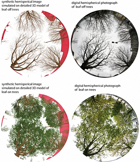Showing the described capabilities, RTMs can improve the integration between traditional monitoring and modelling techniques [7]. For the facilitated comparison with DHPs, such approaches are used in order to simulate synthetic hemispherical images (SHI) on the basis of LiDAR point cloud data [9,21,33]. Thereby, the approaches range from complex ray tracing strategies to simple coordinate transformations into a spherical reference system. Hancock et al. [22] use tLiDAR data in order to simulate the energy distribution which is returned within the laser beam cross-section of an aLiDAR instrument. RTMs offer the advantage of systematic analysis of object sensor relationships for various virtual sensor characteristics and settings, which improves the understanding of a sensor in a given forest domain.

While the advantages of RTM based approaches are obvious, there are some limitations, when LiDAR data are directly integrated into a modelling scene. Most critical are these limitations for tLiDAR data, where a very high geometrical detail is aimed: On the one hand, there is no reliable measure available on how each individual LiDAR point is contributing to the total leaf and plant surface area and to the attenuation of light. To overcome this, each point has to be converted into a spherical solid object, whereby the sphere radius is adapted to the LiDAR beam radius, the distance to the scanner and the return intensity of the point (e.g., [9,21]). Musselman et al. [7] converted tLiDAR data into a voxel structure. Alexander et al. [8] converted a hemispherical field of view into discrete pyramidal structures, in order to obtain an occluding surface area from the point cloud data. These approaches are strongly affected by the resolution of the mentioned voxels and pyramids. On the other hand, a direct use of LiDAR data has to deal with a certain amount of noise. Branches and leaves might be only partly hit by the laser beam cross section. In this case, a part of material located at the edge of the laser beam cross section leads to a point stored at the centre line of the laser beam, which induces an overestimation of object silhouettes and thus canopy closure [34].

Raw point cloud data provide no ready to use object information. Thus, no discrimination of LAI and the total Plant Area Index (PAI) is possible. This inhibits the discrimination of, e.g., solid and porous canopy elements [21] and the consideration of varying object reflectance. Single tree delineation could also improve the estimation of object surface sizes with respect to the branching architecture of a tree.

Most of the described limitations can be overcome with non-trivial reconstruction approaches, which already showed first success [21]: the L-Architect approach by Cote et al. [35,36,37,38] is a hybrid method for the detailed architectural vector modelling of single trees. The resulting polygonal plot reconstructions are promising due to their robustness towards object occlusions and noise in the input data. The approach extracts and reconstructs the basic branching architecture from tLiDAR data as a pipe model, defining a reliable basis for further procedural modelling. Exploiting tree crown inherent topological, point density and lighting information, a set of plausible production rules for twig- and foliage modelling, comparable to a Lindenmayer system [39], is derived. The result is a virtual polygonal tree model following the architectural characteristics of the scanned real tree. In contrast to the raw point cloud data, foliage and wood distributions are decoupled from the pure tLiDAR point measurement densities. Both materials are represented as polygonal meshes, optimized for ray tracing based routines and able to overcome the above-mentioned limitations of surface size definition. Wood elements are treated as cylindrical solids and a robust description of branch radii is given by the pipe model approach [40,41]. Leaves and needles are stored as polygonal objects of defined size. The models allow direct queries on modelled biomass and leaf area in the virtual domain and therefore could provide a plausible approximation of true LAI distributions. However, as stated by Hancock et al. [21], the basic method is not yet practical for characterizing larger areas especially in dense stands with overlapping crowns.

1.1. Main Goals and Applicability

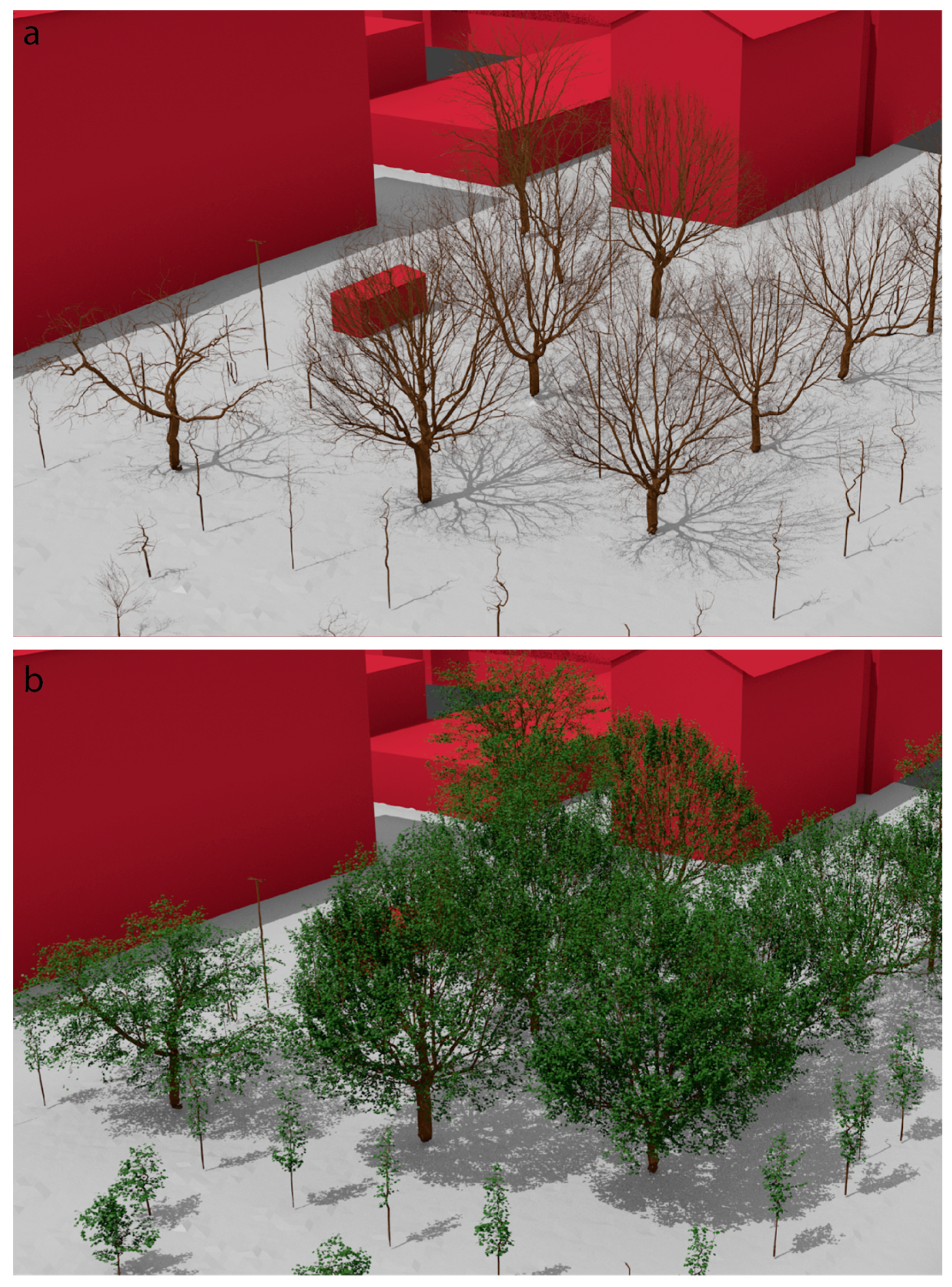
We propose a strategy for target-oriented and detailed forest plot reconstruction, able to fully describe both 3D leaf and plant surface areas in the form of polygonal meshes. Leaf and branch surfaces should be treated separately.

Most regional methods such as aLiDAR-approaches need to be calibrated by plausible plot data in order to be able to estimate LAI and canopy transmissivity. Supporting such calibration and validation scenarios for selected plots within a regional project is one major application of the presented approach.

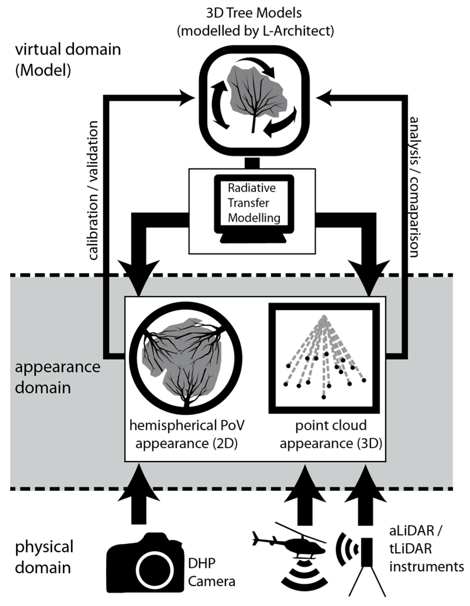
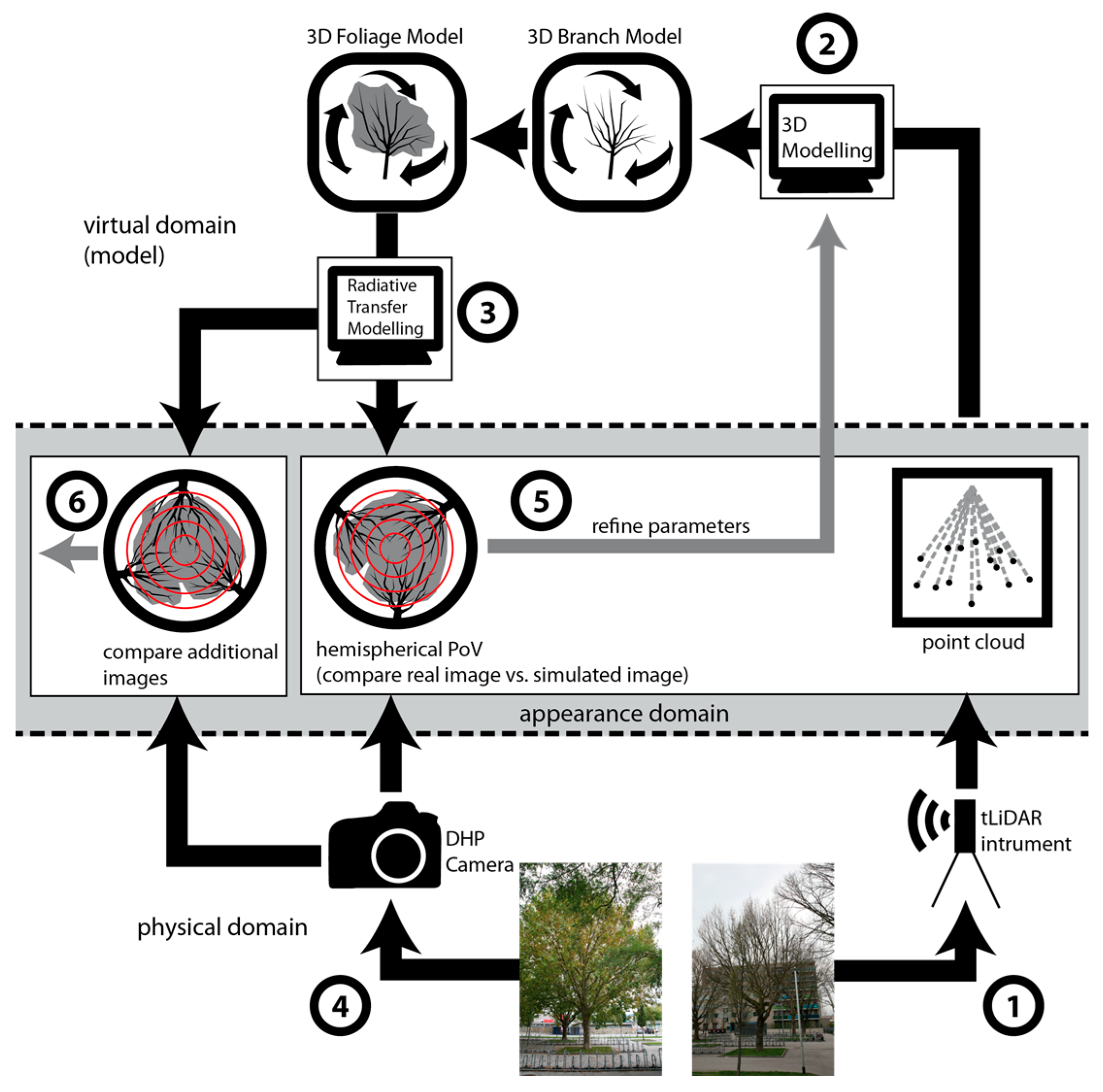
Thereby, the integration of various object appearances captured by different sensors is aimed. As shown in Figure 1 we distinguish between three conceptional domains: (i) the physical domain, which can be measured by various instruments and sensors; (ii) the virtual domain, in which instruments and sensors can be simulated in combination with detailed 3D models coming from the suggested 3D plot reconstruction; and (iii) the appearance domain containing both the real sensor and simulated data for comparison and evaluation. An important goal is to exploit RTM (virtual domain) for the integration of data from different sensors (appearance domain), avoiding the direct comparison of different sensor metrics.

The detailed reconstruction of architectural canopy models as input for the virtual domain is the main focus of the presented paper. The strategy should be optimized in order to derive 3D mesh descriptions of tree crowns from tLiDAR and DHP data in order to be applicable in the virtual domain of a RTM scene.

Fulfilling the described needs, acquisition efforts should be kept as small as possible: if the branching geometries (based on tLiDAR data) are reconstructed and available in the virtual domain, the generation of various foliage densities should be controlled by DHPs only, allowing flexible photo acquisitions and rapid updates of the 3D canopy models without a need for additional tLiDAR campaigns. We aim at a user-friendly and highly automatic derivation of complex canopy and tree parameters for a whole set of trees and not for single trees only.

In order to reach the above-mentioned goals, we rely on three hypotheses which have to be validated:

Hypothesis 1.

The reconstructed leaf-off 3D branching structures show no bias according to the object sensor relationship.

Hypothesis 2.

As procedural foliage modelling is constrained by the 3D branching axes of the 3D model, calibration and validation by multiple DHPs leads not only to correct foliage distributions in the hemispherical views, but also in 3D (including effects of layering and clumping).

Hypothesis 3.

Simulating aLiDAR data based on the modelled polygonal meshes allows systematic analysis of the object–sensor relationships.

1.2. Overview

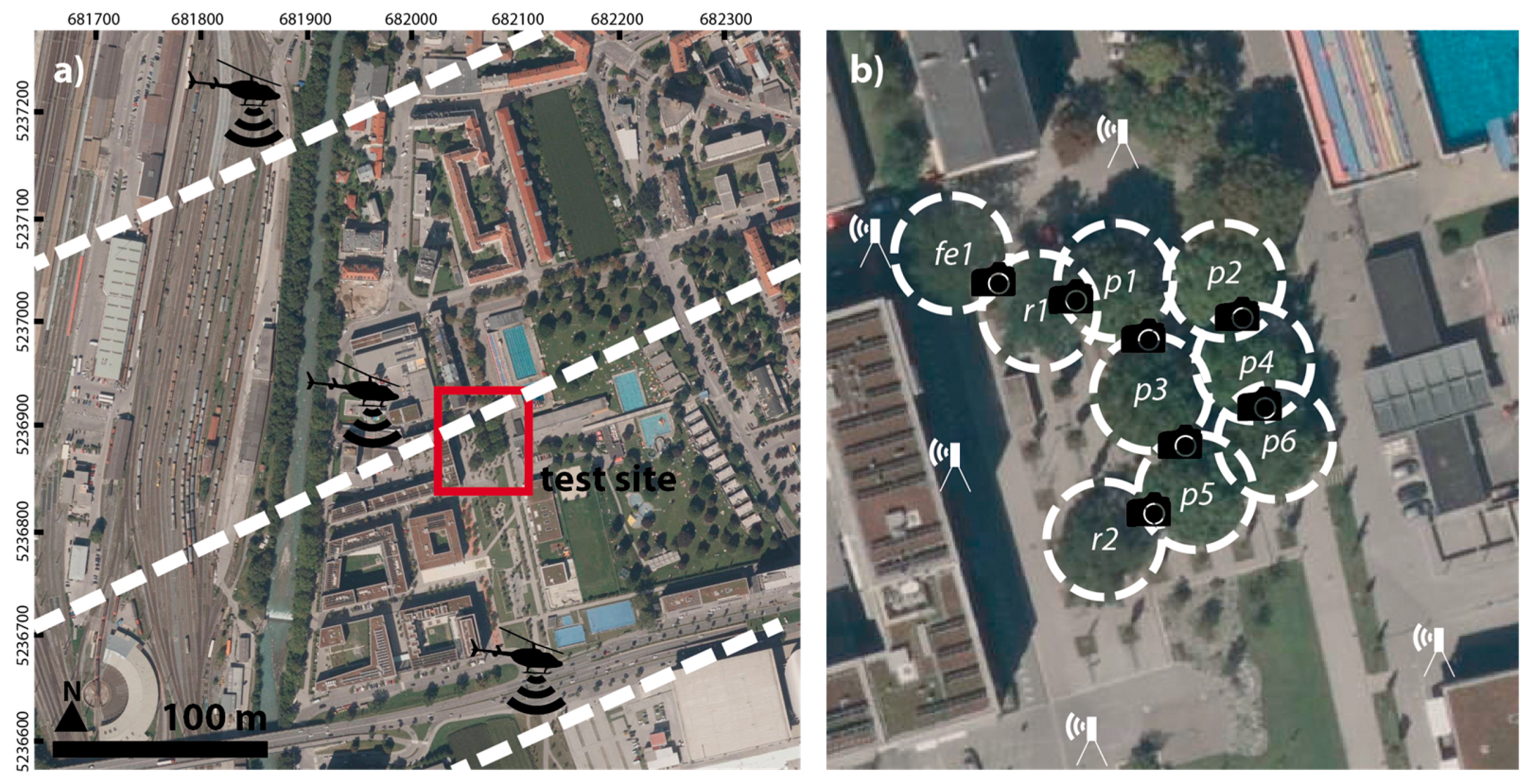
In order to validate the given hypotheses and to show the capabilities of the suggested strategy, we build a controlled exemplary test set up, described in Section 2. In Section 3, we present the methods section. In Section 3.1, the branch reconstruction and foliage modelling method, which is an adaptation of the L-Architect approach [35] is described. In Section 3.2, calibration and validation by DHPs is described in detail. In Section 3.3, the data analysis techniques are described. Respective results of the proposed strategy are presented in Section 4 and discussed in Section 5. Section 6 draws some conclusions.

2. Datasets

The experimental test site used in this study is a 40 × 50 m plot in an urban park environment in the city of Innsbruck (Austria). The test site is located at WGS84 UTM 32T 682054 5235688. It includes nine mature trees with distinct spherical crown shapes of solitary trees. The analysed area includes one ash tree Fraxinus excelsior (fe [tree 1]), two Robinia (r [tree 1,2]) and six plane trees Platanus (p [tree 1–6]).The area of interest is surrounded by younger oak trees (Quercus rubra), which were not analysed in this study due to incomplete coverage.

2.1. Airborne LiDAR Data

aLiDAR data were acquired on 16 October 2012 under leaf on conditions. The point cloud data were acquired using a Eurocopter AS350 with a Riegl LMS-Q680i LiDAR instrument on board. The experimental test area was covered by three overlapping scan strips: one nadir strip with maximum scan angles of 5° and a flying height above ground of 580 m and two neighbouring strips with scan angles between 20° and 30° and flying heights of 629 and 592 m above ground (Figure 2a).

The single strip first return density is 8–10 pts/m² in flat terrain, leading to point densities between 24 and 30 pts/m² in triple overlapping strips. Within the tree crowns, a maximum of seven returns per pulse has been recorded.

2.2. Terrestrial LiDAR Data

tLiDAR data were acquired on 17 April 2015 under leaf-off conditions. The point cloud data were acquired with a Riegl VZ-6000 instrument. The instrument works at 1064 nm wavelength. The trees of the test area were scanned from five scan positions with a vertical and horizontal angular scan stepping of 0.02 degrees and a beam divergence of 0.5 mrad (Figure 2b). The five scan positions show between 21 and 33 M points each. The point cloud data were co-registered into a merged point cloud using the Software LIS Pro 3D [42], applying the techniques given by Horn [43] and Besl and McKay [44]. Using the same registration approach, the merged point cloud was geo-referenced by aligning the tLiDAR point cloud with the aLiDAR point cloud using prominent building edges. This very accurate registration was the main reason for choosing an urban test site for analysis. For the tLiDAR registration the Root Mean Square Error (RMSE) of the alignment is 0.02 m and for the alignment with the aLiDAR it amounts to 0.03 m.

2.3. Digital Hemispherical Photographs

DHPs were acquired with a Canon EOS 5d standard digital photo camera and a Sigma 8 mm F3.5 EX DG circular fisheye orthographic lens. A leaf-off situation was acquired on 17 April 2015 and a leaf-on situation on 8 October 2015.

3. Methods

3.1. Derivation of Branch and Foliage Model

The branch model was derived from the tLiDAR input data by an adapted procedure based on the L-Architect approach [35] and a calibration and validation based on DHPs. An overview of the procedure is given in Figure 3.

3.1.1. Tree Modelling Approach

After tLiDAR acquisition and registration (Figure 3, Step 1), the tree modelling procedure was done using the software LIS Pro 3D [42] including a Tree Growing and Foliage Modelling tool based on the L-Architect approach [35,36,37,38] (Figure 3, Step 2). The tLiDAR data were pre-processed using a progressive TIN-Densification for ground filtering [45]. This was followed by the suggested tree modelling procedure, requiring the six user given input parameters listed in

Table 1. List of user given parameters for the modelling workflow.

Input Parameter	Used Setting
PCAmin 1	0.1 m
PCAmax 1	1.0 m
edge length 2	0.1 m
segment resolution 2	0.2 m
step width 3	0.04 m
light threshold 3	4

¹ defined by expected tree characteristics, ² defined by point cloud quality, ³ calibrated by DHPs.

and explained in the following sections.

At first, tree trunks were detected by a multi-scale pole extraction procedure [46]. The trunk extraction applies a Principle Component Analysis (PCA) on both 0.1 m and 1.0 m radius point neighbourhoods within the point cloud. The two radii (PCAmax and PCAmin) were user defined and adapted to three times the smallest and largest expected tree trunk radius. Doing so, vertical elongated objects were automatically extracted. For all solid elongated objects (by default), trunk diameters were measured in the tLiDAR data by fitting circles into a 0.1 m height slice at breast height. The lowest points of the extracted elongated objects were used as seed points for tree modelling.

For each seed point, a 3D branch model was grown along the tLiDAR points, using the skeletonization approach of Verroust and Lazarus [47]. This procedure was controlled by a user given edge length of 0.1 m and a branch segment resolution of 0.2 m. The skeletonization performs a shortest path algorithm on a so-called geodetic graph [47]. In this graph, edges are defined by all point pair combinations of the tLiDAR data which are defining an edge shorter than the given edge length. The edge length has to be set to the approximate size of point cloud data gaps. The segment resolution defines the length of the branch segment subdivision in the output tree models. The skeletonization processed all given seeds in parallel on a single geodetic graph. Where tree crowns overlapped, crown elements were automatically associated to a trunk position by the evaluation of shortest path distances. This created single tree branch models, directly from ground filtered tLiDAR plot data.

For the modelling of branch thicknesses the measured trunk thicknesses of the extracted pole features were automatically combined with the pipe model approach [40,41] in order to model realistic branch tapering. Realistic branch tapering is an important issue for the use of the models in RTM. The pipe model approach states, that the cross-sectional area of a parent branch in a tree topology equals the sum of the cross-sectional areas of its children. The branching geometry is reconstructed as a set of branch segments, where each is stored as a prism with five polygonal faces. The tree modelling procedure was done for all extracted seed points of the data set and required no calibration.

In our specific urban domain, road signs and lamps were included. Evaluating the branching topology of the reconstructed objects, trees could be discriminated from lamps and road signs as they showed maximum branching levels >4, which was not the case for non-tree objects.

3.1.2. Foliage Modelling

Based on hypothesis 1, the modelled branch models were treated as realistic reconstructions. For all reconstructed tree models, foliage was added by procedural modelling. The modelling procedure was completely automatic and required the two user given parameters step width and ray threshold, which could be automatically found by calibration with a set of DHP images (Section 3.2). All additional parameters are fixed in the used implementation. In the modelling procedure of Platanus, Fraxinus excelsior and Robinia, buds with a 45° angle to the branch axis were spirally arranged along the branch axis by step-wisely rotating the bud by the golden angle. The actual leaf orientation was defined as the combination of the azimuth direction of the bud and an individual leaf slope angle which is defined by a random variable Ls in the interval [10°, 30°]. The leaf slope angle is independent from the characteristics of the bud. Due to memory consumption issues we chose to reconstruct each individual leaf as a simple square (0.1 × 0.1 m²). For more realism, complexity can easily be increased by using complex leaf and needle shape templates for branch colonization (see [35,36,37,38]), which was not realized in the study at hand.

Following the L-Architect approach, the foliage modelling consisted of two steps and was constrained by the reconstructed architecture of a tree and local light conditions. In a first step, all branch ends were colonized by leaves using a defined step width between consecutive leaves of 0.04 m. The step width was found by a calibration procedure described in Section 3.2. For branch ends no light availability was considered. In a second step, all other branch segments showing less than 4 children were considered for leaf colonization, if a sufficient availability of light was given. In order to estimate light conditions computationally, the centre point of each candidate segment was used as a query point for a simplified local ray tracing computation: a number of nine rays, sampling the upper hemisphere of a point with a constant angular distance to each other, were traced from the query point towards the bounding box edges of the data set.

The ray tracing was done in a simple voxel based representation of the tree models. Therefore, the branching architecture was converted into a voxel representation by storing the summed surface area of the geometries falling into a certain voxel as the voxel value. Thus, the voxel area represents the plant area density r_voxel (m²/m³). Following Cote et al. [35], a voxel edge length of 30 cm is implemented, which shows the best agreement between computational effort and plausibility of the results.

In the case the ray tracing was intersecting one or more voxels, the probability of occlusion (P) was computed according to Beer’s law [48] (see also [35]):

$$P=1-{{\displaystyle \prod }}_{\mathrm{voxel}}\exp \left[-r_{voxel}*S_{voxel}*G_{voxel}\right],$$

(1)

S_voxel is the path length of the ray through the voxel and G_voxel = 0.5 is the projection coefficient assuming a spherical distribution of canopy material. If P is larger than a random variable U in the interval [0, 1], the ray is occluded. If the number of occluded rays in the interval [0, 9] was smaller than a light threshold of four rays (found by automatic calibration), the branch segment was spirally colonized with leaves as described above.

3.2. Calibration and Validation of Tree Modelling Approach Using DHPs

Based on hypothesis 2, we calibrated the foliage modelling parameters step width and light threshold using DHPs. Thus, the overall foliage density is calibrated by the parameterization of the procedural model, while the explicit spatial foliage distribution keeps being controlled by the reconstructed 3D branch architecture. For model calibration, a ray tracing algorithm was applied to the tree model geometries in order to simulate a synthetic hemispherical image (SHI) (Figure 3, Step 3). According to the known interior (projective camera geometry) and exterior (geographic position and orientation) orientation of a given camera (defined by a DHP), for each image pixel a ray of defined orientation was traced from the camera’s focal point through the tree models. If the ray intersected with parts of the polygonal geometry, the image pixel was labelled as canopy. This generated a binary image (canopy; gap).

Real DHPs were acquired for a given date (Figure 3 step 4). The camera poses were manually reconstructed by spatial resection using three image tie points and 3 tie points in the 3D models in order to estimate the approximate position and orientation of the camera. The derived camera parameters were used for step 3. The real DHPs were converted into binary images (canopy; gap) by semi-automatic classification using a simple thresholding approach on the red band of the RGB image.

Steps 3 and 4 allowed us to compare the SHIs of the reconstructed tree model with the DHPs (Figure 3, Step 5): for both images the ratio of canopy and gap pixels were computed for rings of the same zenith angle in the range from 5° to 60° with a step size of 5°. The principle of the ring structures is sketched in Figure 3. In our specific test case, zenith angles larger than 60° were not analysed in order to reduce the effect of visible building facades onto the calibration procedure (this limitation is not applicable in a typical forest plot). By averaging the unsigned gap fraction differences between real DHP and modelled SHI an overall gap fraction difference (GFD) was computed as quality measure.

Within a Brute-Force-Testing, the parameters of foliage modelling (step width between leaves and light threshold value for branch segment colonialisation) were calibrated in order to minimize the GFD between DHP and model SHI. After calibration, the quality of the resulting models was evaluated by using additional DHPs (Figure 3, Step 6) and by measuring the GFD in comparison with respective SHIs.

3.3. Data Analysis Approaches

According to hypothesis 3, the assumed capabilities of the created virtual domain were used in order to study the relationships between simulated and real LiDAR point densities and foliage densities. At first, a synthetic LiDAR point cloud was simulated using the given tree models (Section 3.3.1). Additionally, a real LiDAR point cloud was used for comparison (Figure 4, Step 1).

In order to study relationships between directional transmissivities and foliage densities on the one side and laser penetration metrics on the other side, in Steps 2 and 3, the 3D tree model data were converted into ray interception point clouds (describing the true 3D distribution of light attenuating foliage with respect to a specific solar incidence angle) and into a leaf centroid point cloud (describing the modelled leaf density distributions on a point basis) (Section 3.3.2).

In Step 4, the three datasets of Step 1–3 were analysed in 2D and 3D grid layer stacks. Density analysis has then been conducted, on a cell-by-cell basis (see Section 3.3.3).

3.3.1. aLiDAR-Simulation (Step 1)

We used an exemplary ray tracing procedure in order to derive synthetic aLIDAR point clouds which can be evaluated with real sensed data. In order to simulate various sensor types, e.g., waveform LiDAR, in a future study, the ray tracing procedure could simply be replaced by a more complex simulation scheme (e.g., [31,32]). The ray tracer used in the study at hand, emitted nine rays per simulated laser shot (Figure 5b) in order to consider multiple returns per shot. The nine rays were homogeneously sampling the cone shaped volume of the laser beam with a given beam divergence (γ = 0.5 mrad, Riegl LMS-Q680i). For each of the traced rays, potential object intersections are tested. If a single ray intersects with an object, a return is detected and the distance of the intersection point is stored in a sorted array of return distances. In the sorted distance array, adjoining returns are detected (indicated by different colours in Figure 5b) in order to represent a single return of a larger target. If multiple returns of a larger target are connected, the distances of the single ray traces are averaged to a combined return. For each computed return, the detected distances of the returns are applied to the central ray of the shot. This simulates a certain amount of noise, when smaller targets are only hit partly.

In our study, the aLiDAR-simulation was done in two modes: in mode 1, we used a table of ray directions extracted from the real trajectory data of the given aLiDAR flight. This mode made it possible to retrace each individual laser beam transfer through the reconstructed canopy architecture and to perform a plausibility check of the tree models.

In mode 2, we used a given trajectory line and a given flying height above ground h as basic inputs. These inputs were adapted to the trajectory of the real aLIDAR flight. Additionally, a given speed of the aircraft v = 100 km/h and swath width θ = 60° were defined (see Figure 5a).

In order to answer question 3 of the overview section (Section 2), we conducted a sensitivity analysis using simulation mode 2 by systematically changing the scan angle resolution (θ_step) and the pulse repetition rate (PRR): trajectory data, v and θ were locked and the θ_step was consecutively changed in the interval [0.005°, 0.04°] with an increment of 0.001°. As the cross track point distance (d_cross) below the flight trajectory on the flat ground is defined by Equation (2), we guaranteed a homogeneous scan pattern on the ground by adapting PRR to v and θ_step following the criteria given in Equation (3).

$$d_{cross}=tan\left({\theta }_{step}\right) *h$$

(2)

$$PRR=\frac{\left(\theta *v\right)}{\left({\theta }_{step}*d_{cross}\right)}$$

(3)

$$d_{along}=\frac{\theta }{\left({\theta }_{step}*PRR*v\right)}$$

(4)

3.3.2. Generation of Ray Interceptions and Leaf Centroids (Steps 2 and 3)

In order to be able to analyse the transmissivity of the tree models from different directions, we conducted a ray tracing with parallel rays for incidence angles in the interval [10°, 90°] with an increment of 10° (step 3). The parallel rays were emitted in a homogeneous pattern with a spatial resolution of 0.01 m. If a ray intersected with the model geometries, the intersection point was stored as a ray interception. If the ray did not hit a part of the geometry, it was intersected with a virtual background plane and stored as a background point (e.g., ground point). For each simulated point, the virtual emission position was stored. According to the applied ray pattern, each ray-interception represents an area of 0.01 × 0.01 m. The simulated ray-interception point cloud represents the discretized true 3D distribution of light attenuating foliage for a given incident angle. It describes the distribution of possible light and precipitation attenuation within the tree crowns.

Leaf centroids representing the discretized distribution of true LAI were generated by computing the centroid of the polygonal shape of each leaf of the 3D model (step 4).

3.3.3. Spatial Analysis (Step 4)

We analysed the point density measures of simulated aLiDAR points, leaf-centroids and ray-interceptions with the help of a 2D and 3D grid. On a cell-by-cell basis, we correlated the aLiDAR point measures as a predictor variable with the predicted variables describing LAI and canopy transmissivity defined by the tree models. In a 2D and 3D grid structure, we used a cell size of 2 m for analysis.

2D pixel approach: We analysed the density distributions in a standard 2D raster grid using the FOSS-GIS SAGA [49]:

(i) The leaf centroid point cloud was converted into a reference LAI (rLAI) grid (Equation (5)) by counting the number of points in each cell and considering the fixed leaf size of 0.01 m².

$$rLAI=\frac{0.01*\mathrm{point}\_\mathrm{count}}{{\mathrm{cell}\mathrm{size}}^2}(\frac{{\mathrm{m}}^2}{{\mathrm{m}}^2})$$

(5)

(ii) The ray-interception point cloud was split into canopy and background interceptions. Point density grids were generated for both the canopy and the background points separately. Using map algebra, we computed a reference attenuation coefficient (AC) map (see Equation (6)).

$$AC=\frac{canopy\_point\_coun{t}_{intercept}}{\left(background\_point\_coun{t}_{intercept}+canopy\_point\_coun{t}_{intercept}\right)}$$

(6)

(iii) The real and simulated point clouds were separated into ground and canopy points by applying the progressive Triangulated-Irregular-Network-Densification algorithm [45] implemented in the LIS Pro 3D software. By a gridding procedure, point density grids were generated for both the canopy and the ground points. Using simple map algebra, we computed a laser interception ratio (LIR) map (see Equation (7)). In the 2D grid approach, the LiDAR derived attenuation coefficient (AC_L) equals LIR.

$$LIR=\frac{canopy\_point\_coun{t}_{LiDAR}}{\left(background\_point\_coun{t}_{LiDAR}+canopy\_point\_coun{t}_{LiDAR}\right)}$$

(7)

3D voxel approach: We also analysed the density distributions in a 3D voxel system.

(i) The leaf centroid point cloud was converted into a rLAI voxel grid (Equation (4)) according to the 2D grid approach.

(ii) The ray-interception point cloud was analysed on both point and ray basis. On the one hand, canopy point counts per voxel cell were stored. This represents the number of points which were actually intercepted inside the voxel (inside_point_intercept). On the other hand, the rays, defined by each ray-interception point and its associated emission point (along the aircraft flight path), were intersected with the voxel cells. For each cell the number of intersecting rays was stored. This represents the number of rays theoretically passing through a voxel (theo_point_intercept). For rays which only defined theo_point_intercept for the voxel, we tested if the associated interception point was before (before_point_intercept) the voxel intersection or after. For each cell the number of before_points_intercept was stored. AC is defined by Equation (8).

$$AC=\frac{inside\_point{s}_{intercept}}{\left(theo\_point{s}_{intercept}-before\_point{s}_{intercept}\right)}$$

(8)

(iii) For the real and synthetic point clouds, the trajectory information was used in order to reconstruct the exact emission point per return. This allowed computing inside_points_LiDAR, theo_points_LiDAR and before_points_LiDAR as described above. For the aLiDAR data in the 3D grid, LIR and the AC_L are defined by Equations (9) and (10). According to Durrieu et al. [23], the AC_L is defined by Equation (10) and includes an attenuation correction with depth into canopy.

$$LIR=\frac{inside\_point{s}_{LiDAR}}{\left(theo\_point{s}_{LiDAR}\right)}$$

(9)

$$AC\_L=\frac{inside\_point{s}_{LiDAR}}{\left(theo\_point{s}_{LiDAR}-before\_point{s}_{LiDAR}\right)}$$

(10)

4. Results

4.1. 3D Modelling Results

The results of the 3D modelling approach are shown in Figure 6 and Figure 7. Figure 7 demonstrates the 3D distribution of branches and leaves used to generate the SHIs of Figure 6.Compared to the DHPs, the leaf-off tree models show a plausible branching structure, leading to an average gap fraction difference (GFD) of less than 5% for simulated SHIs. Non-tree objects such as lamps were also modelled as a pipe-model, but did not get foliage assigned. The leaf-on trees also show a plausible hemispherical appearance, leading to a GFD of less than 6.5%. Validation by additional DHPs showed GFDs between 6% and 7%.

Compared to the SHIs, which were directly derived from tLiDAR [9,21] (Figure 8), the simulation of SFIs from the 3D models was easier to handle. The respective GFDs of the tLiDAR based VHIs vary strongly according to the applied dot size of each point. Additionally, the discrimination of porous and solid objects is not possible.

4.2. Correlation between Simulated and Real aLiDAR Point Cloud

The synthetic point cloud, which was simulated based on the trajectory information of the real aLiDAR flight and the derived 3D models (mode 1), showed good agreement with the real aLiDAR point cloud.

Correlating the voxel cell based point density observations of both point clouds in a 2 m resolution voxel grid led to an average R² of 0.81. Regression lines were fitted separately for each tree. It can be shown that the regression functions show strong similarities. The scatter plot of the correlation with separate regression lines per tree is shown in Figure 9. The average RMSE between the fitted single-tree regression lines was less than 0.4 pts/m³.

4.3. Correlation between aLiDAR Penetration Metrics and 3D Model Densities

The predictive ability of the aLiDAR penetration metrics to describe foliage densities is varying with the chosen analysis approach and the number of point samples per observation.

4.3.1. 2D Pixel Approach

In the 2D pixel approach, a number of density measures is analysed in a 2D grid cell of infinite vertical extent. With a reference cell size of 2 m, the average laser point count per cell is 106 points (pts) with a triple strip overlap and 52 pts with single strip and the average number of leaves is 999. With a simulated leaf size of 0.01 m² the rLAI value per cell is 2.49 m²/m².

For the described scanning setup the LIR is well suited for the prediction of rLAI. With 2 m cell size, the R² of the correlation between LIR and the number of leaves is in the same range for multiple and single strip coverage (0.79, 0.81).

The fitted regression line for the 2 m cell size setup follows the function given in Figure 10a. With 1 m cell size, the R² decreases to a value of 0.74 (single strip) and 0.68 (triple strip overlap).

With both 2 m and 1 m cell size, the R² of the correlation between AC_L and the true AC at 0° incidence angle is higher than 0.98 (single and overlapping strips). The fitted regression line for 2 m cell size setup follows the function given in Figure 10b.

4.3.2. 3D Voxel Approach

In the 3D voxel approach, density measures were analysed in a 3D grid cell with defined extent in x, y and z direction. With a reference cell size of 2 m, the average laser point count per cell is 28 pts (triple strip overlap) and 15 pts (single strip). The number of rays which are theoretically passing through a voxel cell is 130 (triple strip overlap) and 64 (single strip). The average number of leaves is 283. With a simulated leaf size of 0.01 m² the rLAI value per cell is 0.7 m²/m².

The LIR shows a low ability for the prediction of rLAI. With 2 m cell size, the R² of the correlation between LIR and the number of leaves is 0.40 (single strip) and 0.60 (triple strip overlap). The derived correlation function is given In Figure 10c.

In contrast, the AC_L shows a high ability for the prediction of true AC when penetration is simulated with small incident angles (0.78 (single); 0.82 (overlap); incidence angle = 0°). For moderate incidence angles, the predictive power of the AC_L decreases to R² values of 0.6. For incidence angles ≥60°, the R² decreases to values between 0.5 and 0.4.

4.4. Scan Parameter Simulation

Simulating first return point densities between 2 and 80 pts/m² per strip, AC_L and LIR were computed for both analysis approaches and correlated to true AC and LAI measures given by the 3D architectural tree models. In general, the correlation coefficients show an increase with increasing LiDAR point densities. This is true for both the correlation of rLAI vs. LIR and AC vs. AC_L. The R² values increase along a saturation curve (Figure 11).

For the 2D pixel approach, this effect is less dominant. The range of R² values for the whole test case is very low (0.05 rLAI vs. LIR; 0.01: AC vs. AC_L). R² values for 2 m cell size are high for both low and high point densities (0.80: rLAI vs. LIR; 0.98: AC vs. AC_L).

For the 3D voxel approach the R² values of the rLAI-LIR relationship are very low for small point densities (0.21: 2.1 pts/m²) and reach a maximum of 0.6 at 30 pts/m² with a triple strip overlap. The maximum for a single nadir strip is also reached at 30 pts/m² but is limited to a maximum of about 0.50.

For the AC-AC_L relationship the R² ranges from 0.30 (2.1 pts/m²) to 0.83 (20 pts/m²) with triple strip overlap and a penetration incidence angle of 0°. After reaching the maximum, the R² value keeps almost constant. For larger incident angles the maximum R² value is increasingly damped. For incidence angles smaller than 50° the maximum R² values are still higher than 0.6. For incidence angles ≥60° the R² shows only a maximum of about 0.5.

5. Discussion

5.1. Plausibility of Derived 3D Models (Validation of Hypotheses 1–2)

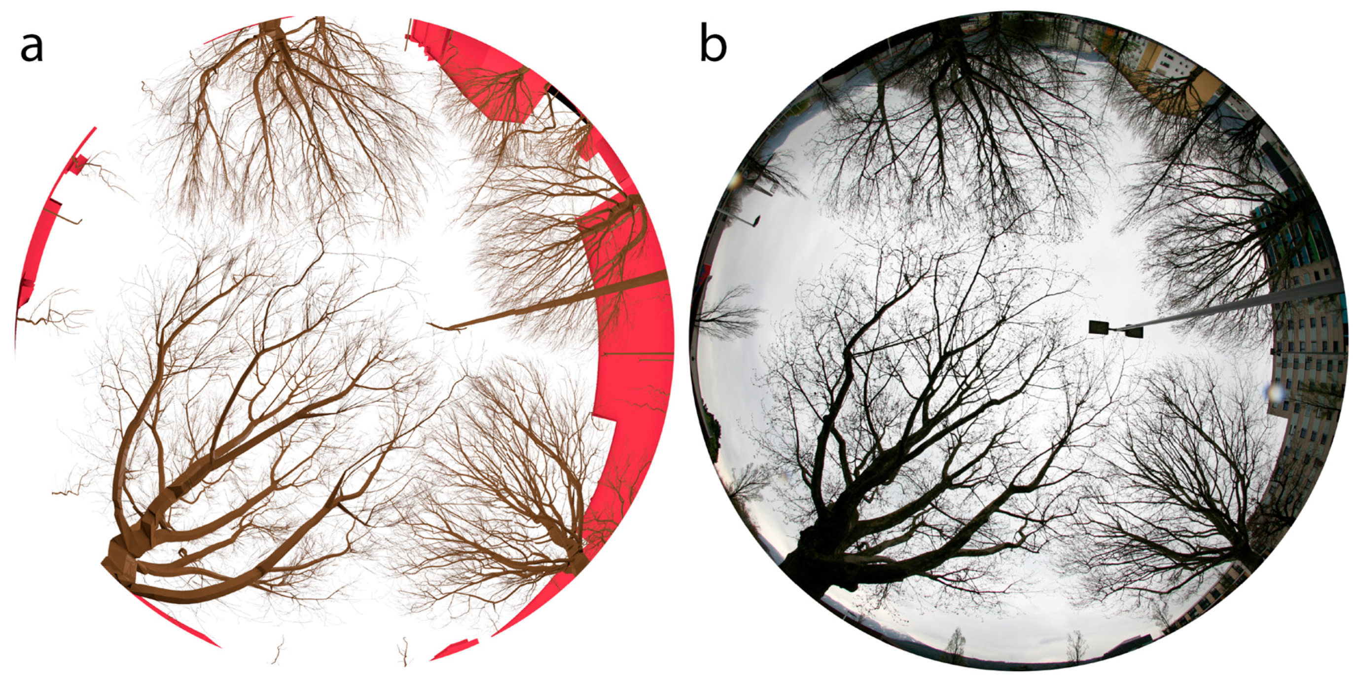
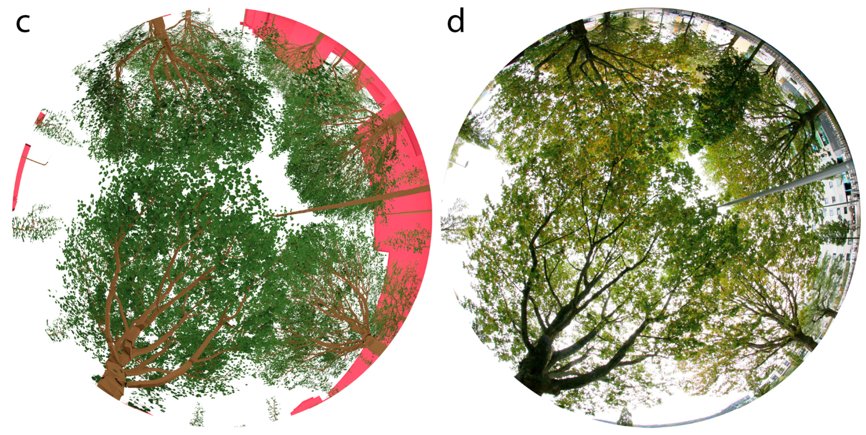
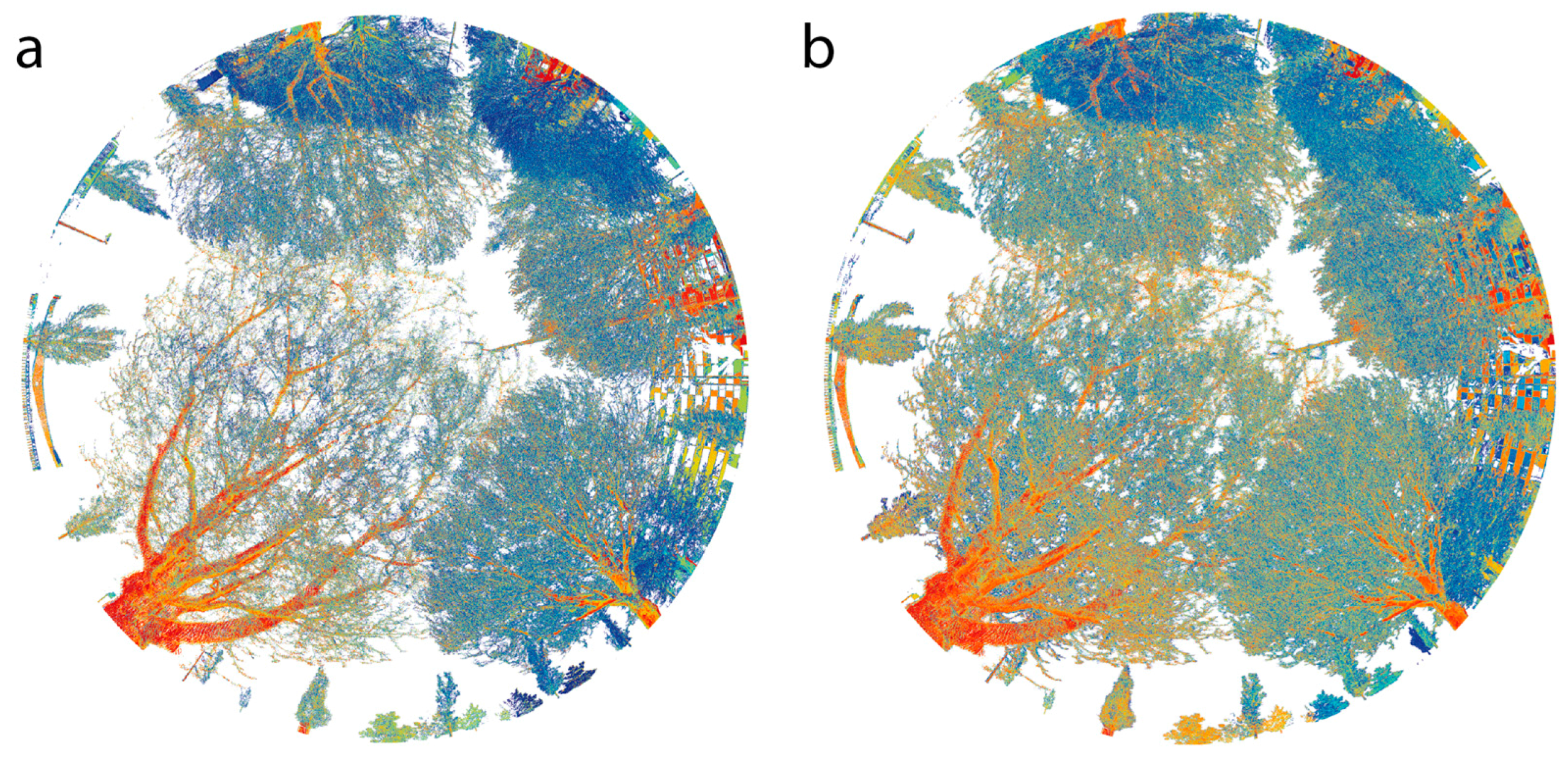
In Section 4.1 and Section 4.2, it could be shown that the analysed 3D tree models (derived by the presented approach) led to plausible GFDs for multiple SHI-DHP comparisons (6%–7% GFD). This was especially the case for the leaf-off case, validating hypothesis 1 (Section 1.1), which states, that the branching models show almost no bias. Section 4.1 shows that the calibration process led to a foliage distribution, which agrees with the DHPs of multiple fields of views. This supports hypothesis 2, stating that DHPs can be used in order to calibrate and validate the characteristics of the modelled 3D models. Looking at the quality of SHIs derived from the 3D models, a facilitated generation is possible, while leaf and branch surface sizes are well defined and stored in a mesh structure. The advantages of such data representation become clear, when these VHIs are compared to SHIs directly derived from tLiDAR data (see Figure 6 and Figure 8).

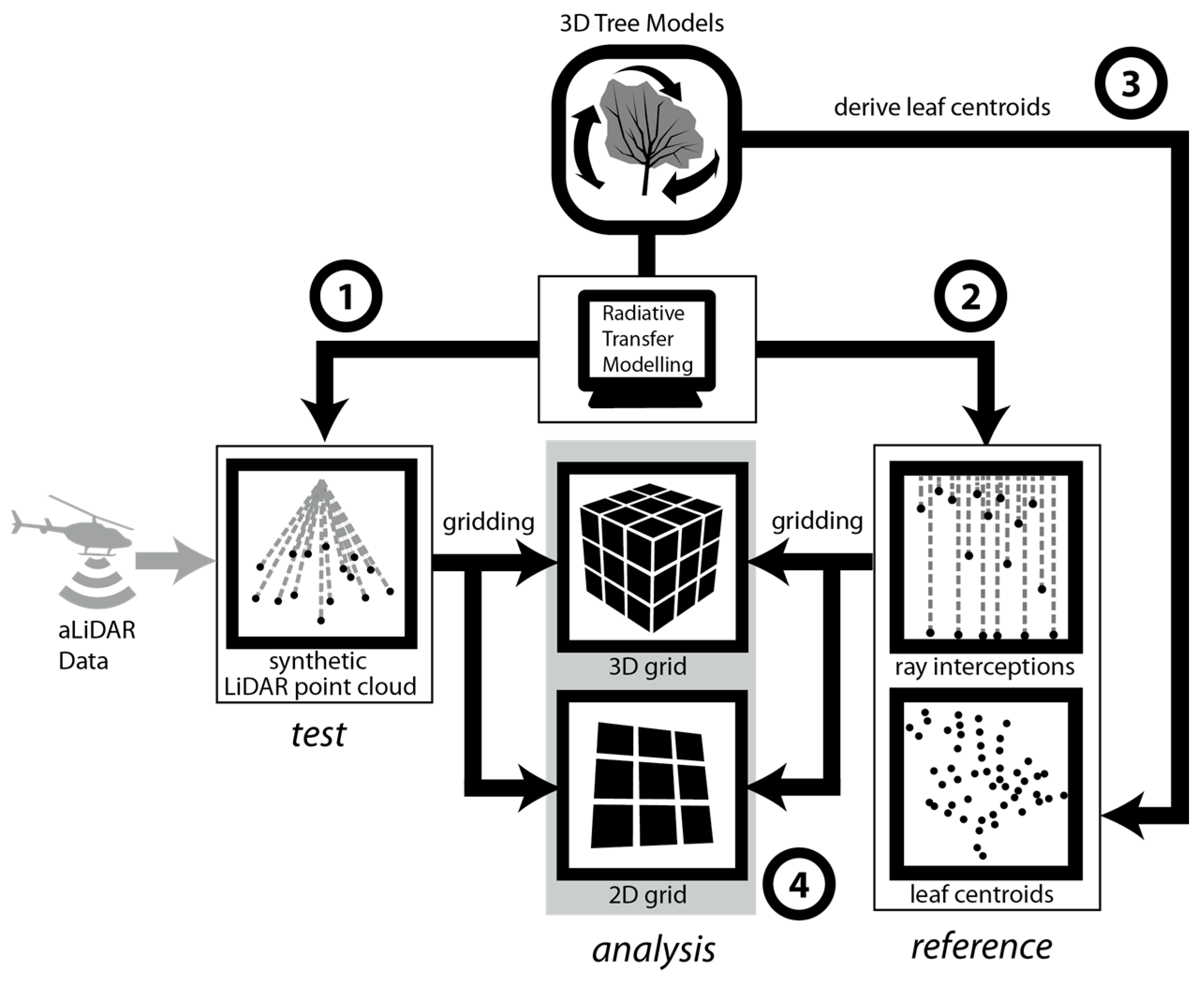
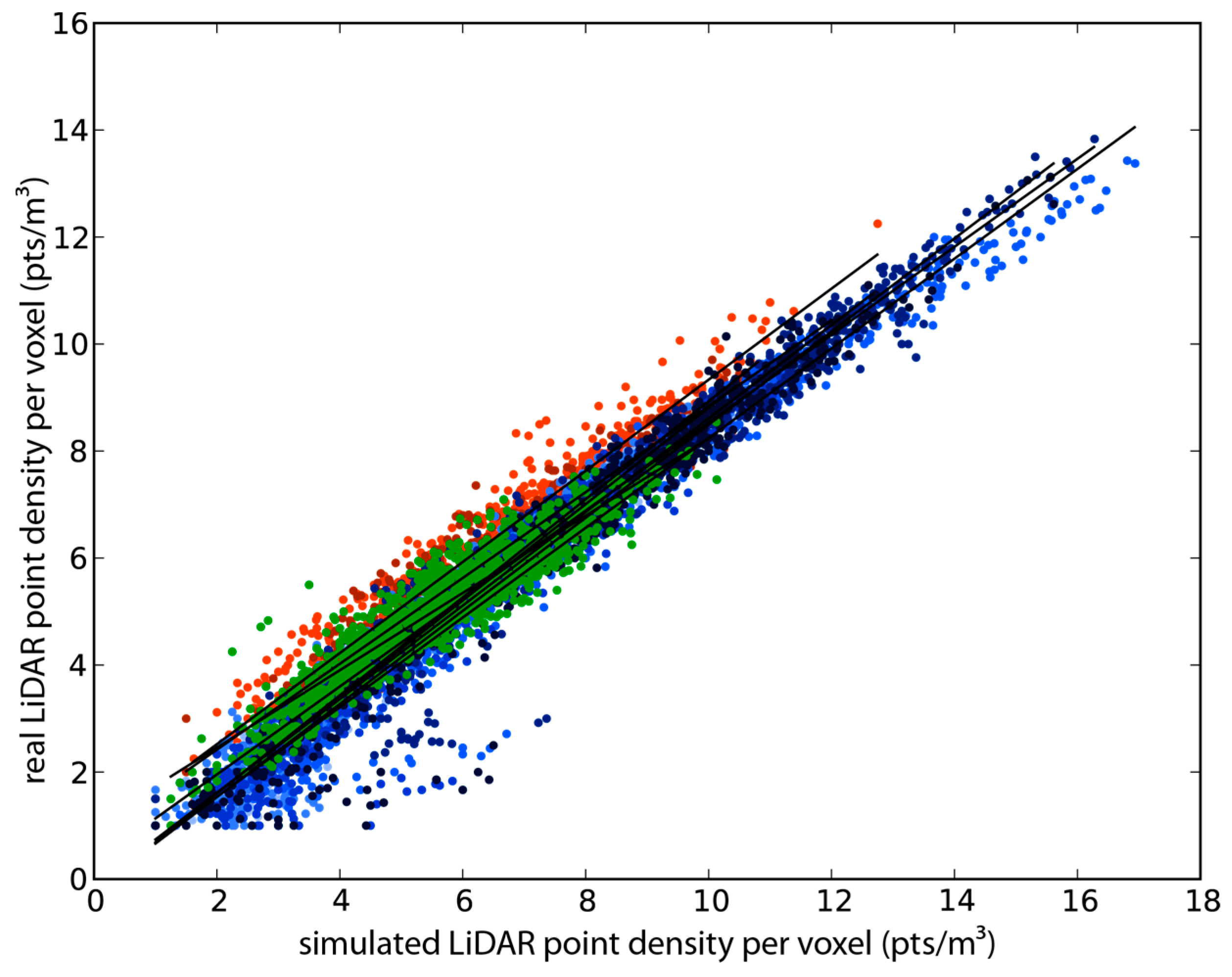
The comparisons of synthetic and real LiDAR data show that plausible aLiDAR point densities were simulated using the presented workflow (R² of 0.81 for the correlation between synthetic and real LiDAR data). This can approve the plausibility of the described setup. Thus, the described set of unknown error sources must show only a negligible influence, which validates the given hypotheses 1 and 2. As the average correlation coefficient was 0.81, Hypothesis 3 could also be validated, stating that the derived 3D model setup is suitable for the systematic simulation of aLiDAR sensors. As the simulated aLiDAR point cloud shows strong similarities to the real data, we can assume a correct representation of the interactions of real foliage densities and the aLiDAR acquisition physics for our model.

The multi-view DHP validation strategy (Figure 3, Step 6) for the modelled data narrows down the pool of error sources approximating the true proportion of errors. A combination of multiple views and sensors minimizes the proportion of uncaptured tree characteristics. Achieving good results for all validation datasets, allowed us to validate the plausibility of the derived virtual domain and thus of the given hypotheses.

It has to be stated, that the suggested strategy is not able to represent a real ground truth. A real ground truth can only be provided by destructive harvesting. Relying on object signatures only, the real canopy status and capturing geometries for both field and flight campaigns remain unknown. However, the strategy represents an additional technique for reference data collection, trying to combine the advantages of tLiDAR and DHP data with those of 3D polygonal mesh representations with attached object information. Thus, it can be used for the calibration and validation of regional scale data. Moreover, the validated 3D models can be used for systematic analysis in a standalone virtual domain (virtual experiment). As a “virtual ground truth” they will permit the comparison of simulated data with the input data of simulation (3D foliage arrangement). This might allow the systematic assessment of the potential of specific physically-based sensors (e.g., discrete return aLiDAR) in a complex RTM [31,32] for the estimation of foliage densities. Additionally, the influences of specific acquisition setups onto the predictive power of sensor metrics can be assessed, serving as a helpful tool for the planning of a flight campaign.

5.2. Prediction of Foliage Densities by Simulated aLiDAR Data

In order to show the potential of the 3D models for usage in a “virtual experiment”, we evaluated the capabilities of simulated aLiDAR data for the prediction of virtual foliage densities (virtual truth). It was demonstrated that systematic relationships between foliage densities and simulated data can be analysed in detail. The given results are exemplary for the given discrete return simulation approach. They show that it is possible to predict both rLAI and AC by LIR and AC_L derived from simulated aLiDAR.

When the determinants of correlation are used for the evaluation of the relationships, the limiting factors are mainly the number of point samples per analysis unit (voxel or pixel) and the number of acquisition directions. The number of point samples is defined by the scanning parameters, leading to a given first return density per m².

The number of acquisition directions is limited by the flight protocol of the simulated campaign, defining the number of overlapping parallel and cross-strips.

In general, AC is predictable with a higher reliability than rLAI, which is due to the acquisition geometry of the aLiDAR. Especially for close nadir laser shots, the sampling geometry is very similar to a vertical penetration of precipitation or light and its respective attenuation coefficient. With higher incidence angles of ray penetration, the sampling geometries become increasingly different, leading to a decrease in predictive power. Essentially, incoming parallel light with high incidence angles interacts with a completely different object silhouette than incoming laser light (with close nadir directions). One possibility to study the magnitude of this effect is to use a virtual experimental setup for detailed RTM. Such a virtual experimental setup has been used in the presented experiment.

rLAI predictions in general show lower predictive power than AC predictions, but improve when multiple strips are used. While the distribution of AC shows no multi-layering orthogonal to the penetration direction, rLAI shows strong vertical layering. This can be quantified using the given 3D model set up, which includes a plausible representation of vertical canopy layering.

Comparing the 3D model and the simulated point cloud data allowed us to quantify an improvement of rLAI predictions with the use of multiple scan strips. This is not only due to a simple increase in point sampling but also due to an improved capture of the multi layered distributions of rLAI with multiple strips: For a single strip, only one dominant penetration direction is considered, increasing the probability of under-sampling of the multi-layered tree crown. With triple strip overlap, the object is captured by a combination of smaller and larger incidence angles from three different trajectories. If rays, coming in from one direction, are not able to penetrate to a certain position of the tree crowns, another set of rays, coming from another direction, have the chance to penetrate to this position and sample the foliage density. This decreases the probability of under-sampling of the multi-layered leaf distribution. For a perfect sampling of this rLAI distribution, an infinite number of viewing directions would be needed. In Section 4.4 it can be shown that the maximum correlation coefficient describing the relationship between rLAI and LIR is limited to 0.8. However, as could be shown in previous work, realistic LAI estimates can be derived from waveform LiDAR [29,30]. In an enhanced virtual experiment, these capabilities could be proofed by using 3D models in combination with a waveform LiDAR simulator [32] exceeding the scope of this paper.

5.3. Comparison of Data Structures for Analysis

Comparing the analysed data structures (2D grid, 3D grid) by the determinants of correlation for the density predictions, the voxel data structure was the more problematic description. Compared to the pixel approach, this is mainly due to the smaller size of the voxel analysis unit compared to the pixel analysis unit of the same cell size. 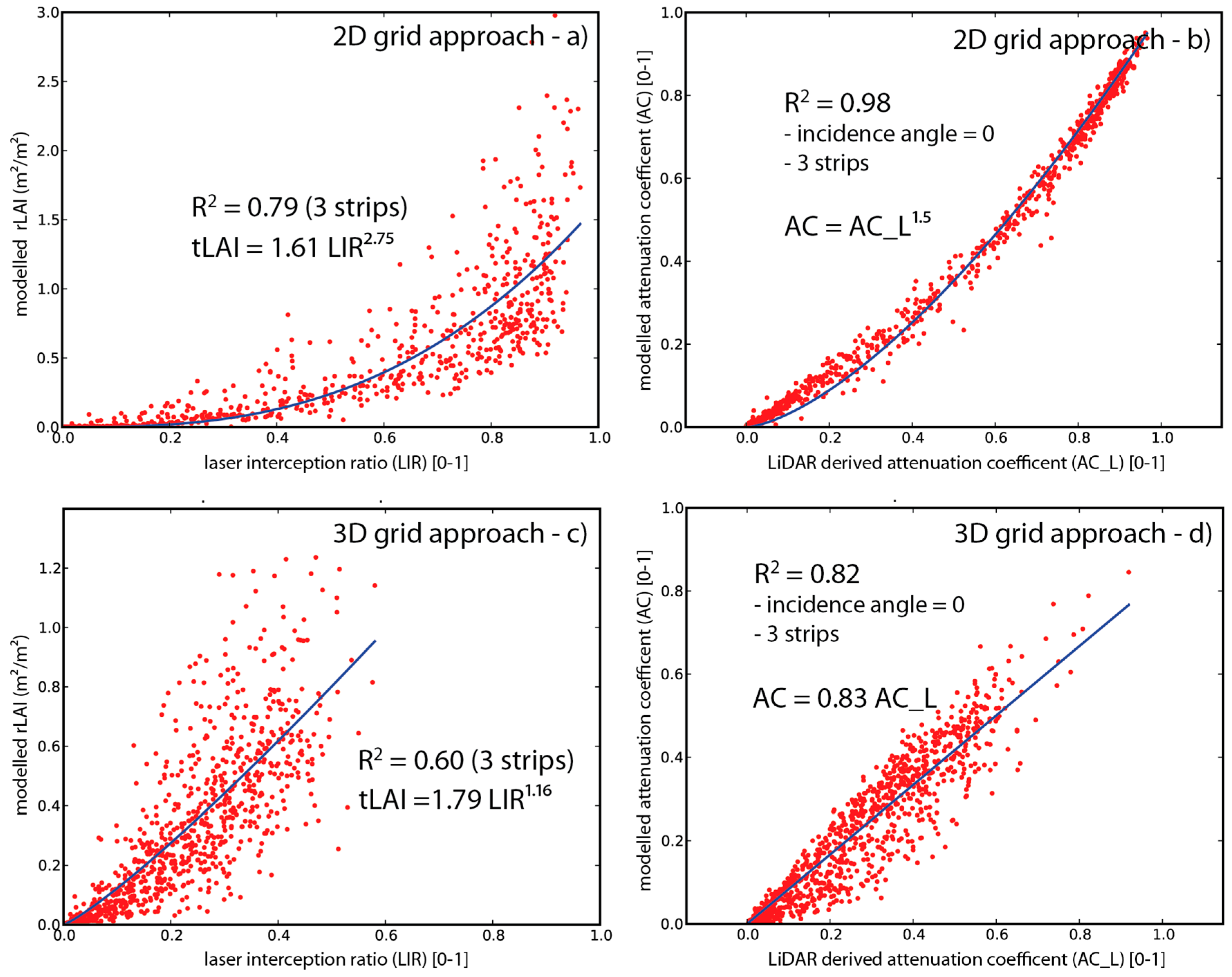As a smaller analysis unit the voxel shows an average point count which is only 30% of the average pixel point count (Section 4.3). This implies a smaller number of samples per analysis unit leading to more noisy observations compared to the pixel unit, where the reduction of noise by averaging is intensified due to an increased number of samples. Neglecting the sampling based effects, it has to be stated, that the derived relationships show linear behaviours for the 3D grid and are slightly biased for the 2D grid (Figure 10). A bias is visible especially with LIR and AC_L values between 0.8 and 1.0. The effect is indicated by higher exponents of the fitting functions. This effect can be explained by the characteristics of the analysis units. The 2D grid represents a vertical column unifying parts of the interior crown, which are problematic in terms of under-sampling, with less critical top canopy parts. This unifying effect does not exist for the voxel analysis unit, which discretizes the vertical density distribution. The vertical discretization allows a correction of attenuation with depth into canopy (see Equation (9) according to Durrieu et al. [23]), which is not possible for the vertically unified 2D grid unit.

5.4. Comparison of Scan Settings and Point Densities for Analysis

In general, it can be stated that the quality of canopy density prediction increases with increasing first return point densities. The number of point samples per analysis unit controls the quality of the predictions. Thus, the decision for a scan pattern is also related to the respective data structure to be used for analysis.

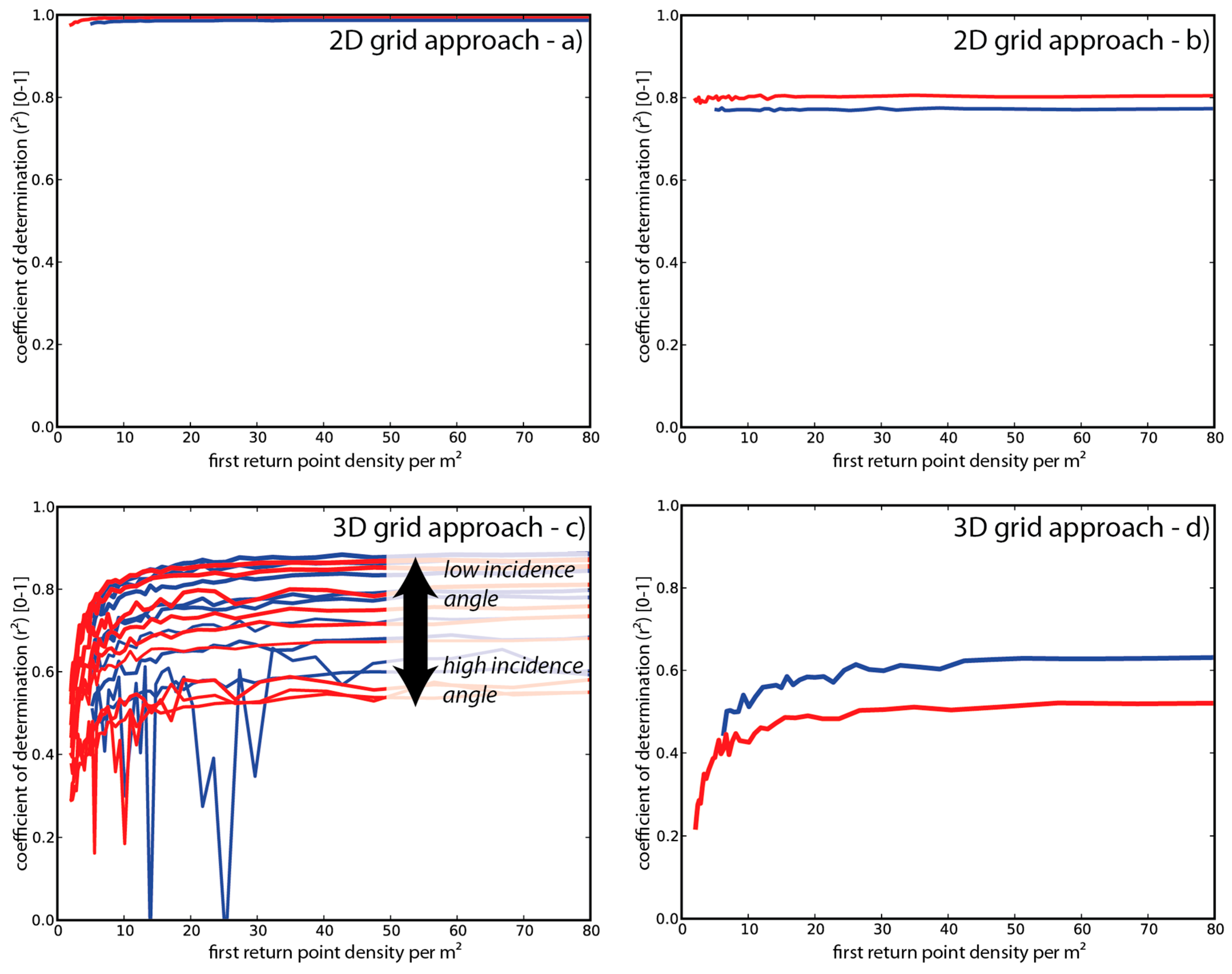
For the 2D data structure, where the vertical density distribution is unified within each pixel and where point sampling densities are sufficient, the predictive power is hardly affected by varying point densities and strip overlaps. This results in correlation coefficients remaining in the same range for all tested setups. As the pixel analysis unit shows a sufficient number of samples for the whole tested range of scan settings, the R² reaches its maximum already at a first return density of 5 pts/m². For AC, which shows no vertical clumping, this leads to almost perfect predictions. The R² of rLAI prediction did never exceed 0.8. This suggests that the quality has reached a saturation level. Sampling density and additional flight strips have a negligible effect onto the quality of the predictions. Only a capturing technique, which is able to sample the inner crown in a homogeneous manner, would be able to further improve the R².

Due to the smaller size of the voxel analysis unit, the increase of predictive power with increasing point density is more pronounced. A sufficient number of sampling points is reached at a first return density of 30 pts/m². For rLAI in particular, this is not enough in order reach an R² higher than 0.6, which can also be explained by the limitations of the object–sensor relationship.

The “virtual experiment” showed that the 2D grid approach was more reliable than the 3D grid approach, especially for LAI mapping. Nevertheless, it has to be noted that the 2D approach aims only at a 2D mapping of LAI ignoring the vertical LAI profile within canopy. In order to achieve this goal, point densities higher than 5 pts/m² are already suitable for 2D LAI description (not significantly improvable with increased point densities). Nevertheless, it has to be stated that with only 4 pts/m², LiDAR based height estimates show errors of up to 1 m, which can lead to errors of aboveground biomass estimates of 80–125 Mg·ha⁻¹ [50]. The 3D grid approach aims at a three dimensional mapping of LAI, which is more ambitious and can only be achieved with moderate predictive power. This suggests the exploitation of more advanced sensing techniques, such as full-waveform LiDAR, which has already been proofed for vertical LAI mapping [29,30].

6. Conclusions

In order to evaluate aLiDAR based canopy metrics, we presented a strategy to upgrade traditional in-situ data such as leaf-off tLiDAR and leaf-on DHP-data into plausible 3D canopy models. Using a highly automated reconstruction and modelling workflow has the advantage of an almost unbiased virtual 3D representation of branch and leaf densities. In contrast to the primary in-situ data, systematic errors due to the object–sensor relationship are minimized (hypothesis 1). Calibration and validation is done based on synthesized (SHI) and real (DHP) canopy signatures of sensed data. As the foliage modelling is constrained by the 3D branching architecture of a tree, calibrating the foliage density for a reference DHP leads to plausible foliage densities also in 3D, which was validated by additional DHPs (hypothesis 2). The plausibility of 3D foliage densities could also be cross-checked by comparing a synthesized and a real aLiDAR point cloud.

It could be shown that the reconstructed models permit the evaluation of aLiDAR based rLAI and AC predictions under various scan settings and different data structures (hypothesis 3). Thereby, the importance of laser point sampling density as well as the diversity of scan angles and their quantitative effect onto error margins became clear. It could also be shown that the improved vertical discretization of foliage density in a voxel structure suffers from a lower sampling resolution defined by a critical number of laser points per analysis unit.

The reconstructed polygonal mesh geometries of the 3D models are predestinated for the development of a RTM scenes, usable for a wide range of simulations.

As the presented approach is based on highly automated workflows for model derivation, it can serve as reference data complementing future regional flight campaigns: tLiDAR data have only to be acquired once. (If the 3D branching framework is created, a practical foliage density monitoring can be done only using DHPs and automatically calibrating and validating the 3D canopy density modelling for the given time step or flight campaign date.)

In future, the strategy could also be used for an extended experimental setup including a broad sample of tree species. Doing so, single tree based allometric functions could be found based on the 3D models and compared to measures from discrete return or waveform aLiDAR and, e.g., optical satellite imagery. This could improve the understanding of canopy metrics and their ability to predict canopy density measures and could support the development of new canopy density metrics and correction functions.

References

1. Calders, K.; Newnham, G.; Burt, A.; Murphy, S.; Raumonen, P.; Herold, M.; Culvenor, D.; Avitabile, V.; Disney, M.; Armston, J. Nondestructive estimates of aboveground biomass using terrestrial laser scanning. Methods Ecol. Evol. 2015, 6, 198–208. [Google Scholar] [CrossRef]
2. Ashcroft, M.B.; Gollan, J.R.; Ramp, D. Creating vegetation densitiy profiles for a diverse range of ecological habitats using terrestrial laser scanning. Methods Ecol. Evol. 2014, 5, 263–272. [Google Scholar] [CrossRef]
3. Clinton, B.D. Light, temperature, and soil moisture responses to elevation, evergreen understory, and small canopy gaps in the southern Appalachians. For. Ecol. Manag. 2003, 186, 243–255. [Google Scholar] [CrossRef]
4. Chen, J.M.; Black, T. Defining leaf area index for non-flat leafs. Plant Cell Environ. 1992, 15, 421–429. [Google Scholar] [CrossRef]
5. Best, M.J.; Pryor, M.; Clark, D.B.; Rooney, G.G.; Essery, R.L.H.; Ménard, C.B.; Edwards, J.M.; Hendry, M.A.; Porson, A.; Gedney, N.; et al. The Joint UK Land Environment Simulator (JULES), model description—Part 1: Energy and water fluxes. Geosci. Model Dev. 2011, 4, 677–699. [Google Scholar] [CrossRef]
6. Clark, D.B.; Mercado, L.M.; Sitch, S.; Jones, C.D.; Gedny, N.; Best, M.J.; Pryor, M.; Rooney, G.G.; Essery, R.L.H.; Blyth, E.; et al. The joint UK environment simulator (JULES), model description—Part 2: Carbon fluxes and vegetation dynamics. Geosci. Model Dev. 2011, 4, 701–722. [Google Scholar] [CrossRef] [Green Version]
7. Musselman, K.N.; Margulis, S.A.; Molotch, N.P. Estimation of solar direct beam transmittance of conifer canopies from airborne LiDAR. Remote Sens. Environ. 2013, 136, 402–415. [Google Scholar] [CrossRef]
8. Alexander, C.; Moeslund, J.E.; Boecher, P.K.; Arge, L.; Svenning, J.-C. Airborne laser scanner (LiDAR) proxies for understory light conditions. Remote Sens. Environ. 2013, 134, 152–161. [Google Scholar] [CrossRef]
9. Moeser, D.; Roubinek, J.; Schleppi, P.; Morsdorf, F.; Jonas, T. Canopy closure, LAI and radiation transfer from airborne LiDAR synthetic images. Agric. For. Meteorol. 2014, 197, 158–168. [Google Scholar] [CrossRef]
10. Tooke, T.R.; Coops, N.C.; Christen, A.; Gurtuna, O.; Prevot, A. Integrated irradiance modelling in the urban environment based on remotely sensed data. Sol. Energy 2012, 86, 2923–2934. [Google Scholar] [CrossRef]
11. Xiao, Q.; MacPhearson, E.G. Rainfall interception by Santa Monica’s municipal urban forest. Urban Ecosyst. 2002, 6, 291–302. [Google Scholar] [CrossRef]
12. Grau, E.; Gastellu-Etchegorry, J.P. Radiative transfer modeling in the earth-atmosphere system with DART model. Remote Sens. Environ. 2013, 139, 149–170. [Google Scholar] [CrossRef]
13. Alonso, M.; Bookhagen, B.; McFadden, J.P.; Sun, A.; Roberts, D.A. Mapping urban forest leaf area index with airborne LiDAR using penetration metrics and allometry. Remote Sens. Environ. 2015, 162, 141–153. [Google Scholar] [CrossRef]
14. Zheng, G.; Moskal, M.L. Retrieving Leaf Area Index (LAI) Using Remote Sensing: Theories, Methods and Sensors. Sensors 2009, 9, 2719–2745. [Google Scholar] [CrossRef] [PubMed]
15. Miller, J.B. A formula for average foliage density. Aust. J. Bot. 1964, 15, 141–144. [Google Scholar] [CrossRef]
16. Nilson, T. A theoretical analysis of the frequency of gaps in plant stands. Agric. Meteorol. 1971, 8, 25–38. [Google Scholar] [CrossRef]
17. Nilson, T.; Kuusk, A. Improved algorithm for estimating canopy indices from gap fraction data in forest canopies. Agric. For. Meteorol. 2004, 124, 157–169. [Google Scholar] [CrossRef]
18. Palleto, A.; Tosi, V. Forest Canopy cover and canopy closure: A Comparison of assessment techniques. Eur. J. For. Res. 2009, 128, 265–272. [Google Scholar] [CrossRef]
19. Korhonen, L.; Korpela, I.; Heiskanen, J.; Maltamo, M. Airborne discrete-return LiDAR data in the estimation of vertical canopy cover, angular canopy closure and leaf area index. Remote Sens. Environ. 2011, 115, 1065–1080. [Google Scholar] [CrossRef]
20. Korhonen, L.; Korhonen, K.T.; Rauitainen, M.; Stenberg, P. Estimation of forest canopy cover: A comparison of field measurement techniques. Silva Fenn. 2006, 40, 577–588. [Google Scholar] [CrossRef]
21. Hancock, S.; Essery, R.; Reid, T.; Carle, J.; Baxter, R.; Rutter, N.; Huntley, B. Characterizing forest gap fraction with terrestrial LiDAR and photography: An examination of relative limitations. Agric. For. Meteorol. 2014, 189–190, 105–114. [Google Scholar] [CrossRef] [Green Version]
22. Hancock, S.; Anderson, K.; Disney, M.; Gaston, K.J. Measurement of fine-spatial-resolution 3D vegetation structure with airborne waveform LiDAR. Calibration and validation with voxelised terrestrial LiDAR. Remote Sens. Environ. 2017, 188, 37–50. [Google Scholar] [CrossRef]
23. Durrieu, S.; Allouis, T.; Fournier, R.; Vega, C.; Albrech, L. Spatial quantification of vegetation density from terrestrial laser scanner data for characterization of 3D forest structure at plot level. In Proceedings of the Silvilaser 2008: 8th International Conference on LiDAR Applications in Forest Assessment and Inventory, Edinburgh, UK, 17–19 September 2008.
24. Jensen, J.J.; Humes, K.S.; Vierling, L.A.; Hudak, A.T. Discrete return LiDAR-based prediction of leaf area index in two conifer forests. Remote Sens. Environ. 2008, 112, 3947–3957. [Google Scholar] [CrossRef]
25. Morsdorf, F.; Kötz, B.; Meier, E.; Itten, K.I.; Allgöwer, B. Estimation of LAI and fractional cover from small footprint airborne laser scanning data based on gap fraction. Remote Sens. Environ. 2006, 104, 50–61. [Google Scholar] [CrossRef]
26. Riano, D.; Valladares, F.; Condes, S.; Chuvieco, E. Estimation of leaf area index and covered ground from airborne laser scanner (LiDAR) in two contrasting forests. Agric. For. Meteorol. 2004, 124, 269–275. [Google Scholar] [CrossRef]
27. Richardson, J.; Moskal, L.M.; Kim, S. Modelling approaches to estimate effective leaf area index from aerial discrete-return LiDAR. Agric. For. Meteorol. 2009, 149, 1152–1160. [Google Scholar] [CrossRef]
28. Solberg, S.; Brunner, A.; Hanssen, K.H.; Lange, H.; Naesset, E.; Rautiainen, M. Mapping LAI in a Norway spruce forest using airborne laser scanning. Remote Sens. Environ. 2009, 113, 2317–2327. [Google Scholar] [CrossRef]
29. Tang, H.; Dubayah, R.; Swantantran, A.; Hofton, M.; Sheldon, S.; Clark, D.B.; Blair, B. Retrieval of vertical LAI profiles over tropical rain forests using waveform LiDAR at La Selva, Costa Rica. Remote Sens. Environ. 2012, 124, 242–250. [Google Scholar] [CrossRef]
30. Armston, J.; Disney, M.; Lewis, P.; Scarth, P.; Phinn, S.; Lucas, R.; Bunting, P.; Goodwin, N. Direct retrieval of canopy gap probability using airborne waveform LiDAR. Remote Sens. Environ. 2013, 134, 24–38. [Google Scholar] [CrossRef]
31. Gastellu-Etchegorry, J.P.; Yin, T.; Lauret, N.; Cajgfinger, T.; Gregoire, T.; Grau, E.; Feret, J.B.; Lopes, M.; Guilleux, J.; Dedieu, G.; et al. Discrete anisotropic radiative transfer (DART 5) for modeling airborne and satellite spectrometer and LiDAR acquisitions of natural and urban landscapes. Remote Sens. 2015, 7, 1667–1701. [Google Scholar] [CrossRef] [Green Version]
32. Yin, T.; Lauret, N.; Gastellu-Etchegorry, J.P. Simulation of satellite, airborne and terrestrial LiDAR with DART (II): ALS and TLS multi-pulse acquisitions, photon counting, and solar noise. Remote Sens. Environ. 2016, 184, 454–468. [Google Scholar] [CrossRef]
33. Varhola, A.; Frazer, G.W.; Teti, P.; Coops, N.C. Estimation of forest structure metrics relevant to hydrologic modelling using coordinate transformation of airborne laser scaning data. Hydol. Earth Syst. Sci. 2012, 16, 3749–3766. [Google Scholar] [CrossRef] [Green Version]
34. Danson, F.M.; Hetherington, D.; Morsdorf, F.; Kötz, B.; Allgöwer, B. Forest canopy gap fraction from terrestrial laser scanning. IEEE Geosci. Remote Sens. Lett. 2007, 4, 157–160. [Google Scholar] [CrossRef] [Green Version]
35. Cote, J.F.; Fournier, R.A.; Egli, R. An architectural model of trees to estimate forest structural attributes using terrestrial LiDAR. Environ. Model. Softw. 2011, 26, 761–777. [Google Scholar] [CrossRef]
36. Cote, J.F.; Fournier, R.A.; Fraser, G.W.; Niemann, O.K. A fine-scale architectural model of trees to enhance LiDAR-derived measurements of forest canopy structure. Agric. For. Meteorol. 2012, 166–167, 72–85. [Google Scholar] [CrossRef]
37. Cote, J.F.; Fournier, R.A.; Luther, J.E. Validation of L-Architect model for balsam fir and black spruce trees with structural measurements. Can. J. Remote Sens. 2013, 39, 41–59. [Google Scholar] [CrossRef]
38. Cote, J.F.; Widlowski, J.L.; Fournier, R.A.; Verstraete, M.M. The structural and radiative consistency of three dimensional tree reconstructions from terrestrial LiDAR. Remote Sens. Environ. 2009, 113, 1067–1081. [Google Scholar] [CrossRef]
39. Lindenmayer, A. Mathematical models for cellular interaction in development, Part I and II. J. Theor. Biol. 1968, 18, 280–315. [Google Scholar] [CrossRef]
40. Shinozaki, K.; Yoda, K.; Hozumi, K.; Kira, T. A quantitative analysis of plant form—The pipe model theory. I. Basic analyses. Jpn. J. Ecol. 1964, 14, 97–105. [Google Scholar]
41. Macdonald, N. Trees and Networks in Biological Models; John Wiley & Sons: New York, NY, USA, 1983; pp. 1–215. [Google Scholar]
42. Laserdata GmbH. Available online: www.laserdata.at (accessed on 17 December 2016).
43. Horn, B.K.P. Closed-form solution of absolute orientation using unit quaternions. J. Opt. Soc. Am. 1987, A4, 629–642. [Google Scholar] [CrossRef]
44. Besl, P.J.; McKay, N.D. A Method for Registration of 3D-Shapes. IEEE Trans. Pattern Anal. Mach. Intell. 1992, 14, 239–256. [Google Scholar] [CrossRef]
45. Axelsson, P.E. DEM generation from laser scanner data using adaptive TIN models. Int. Arch. Photogramm. Remote Sens. Spat. Inf. Sci. 2000, 32 Pt B4/1, 110–117. [Google Scholar]
46. Bremer, M.; Wichmann, V.; Rutzinger, M. Eigenvalue and graph-based object extraction from mobile laser scanning point clouds. ISPRS Ann. Photogramm. Remote Sens. Spat. Inf. Sci. 2013, II-5/W2, 55–60. [Google Scholar] [CrossRef]
47. Verroust, A.; Lazarus, F. Extracting skeletal curves from 3D scattered data. Vis. Comput. 2000, 16, 15–25. [Google Scholar] [CrossRef]
48. Beer, A. Bestimmung der Absorption des rothen Lichts in farbigen Flüssigkeiten. Ann. Phys. Chem. 1852, 86, 78–88. [Google Scholar] [CrossRef]
49. Conrad, O.; Bechtel, B.; Bock, M.; Dietrich, H.; Fischer, E.; Gerlitz, L.; Wehberg, J.; Wichmann, V.; Böhner, J. System for Automated Geoscientific Analyses (SAGA) v. 2.1.4. Geosci. Model. Dev. 2015, 8, 1991–2007. [Google Scholar] [CrossRef]
50. Leitold, V.; Keller, M.; Morton, D.C.; Cook, B.D.; Shimabukuro, Y.E. Airborne LiDAR-based estimates of tropical forest structure in complex terrain: Opportunities and trade-offs for REDD++. Carbon Balance Manag. 2015, 10, 3. [Google Scholar] [CrossRef] [PubMed]
Figure 1. Basic concept. The virtual domain (3D Models) is the digital reconstruction of the physical one. A comparison of model and physical domain can only be done in the appearance domain. The assessment of the physical domain is restricted to a limited set of sensing/measuring techniques that can be simulated in the virtual domain (DHP, tLiDAR, aLiDAR).
Remotesensing 09 00220 g001
Figure 2. (a) Surroundings of the experimental test site, showing the trajectories of the aLiDAR flight strips; and (b) experimental test site showing the tree positions of Fraxinus excelsior (fe [tree 1]), Robinia (r [tree 1,2]) and Platanus (p [tree 1–6]). Scan positions and DHP positions are indicated by the instrument symbols (image source: tiris maps).
Remotesensing 09 00220 g002
Figure 3. Overview of the derivation of the 3D Models: (1) In a leaf-off situation, in the physical domain, a point cloud is acquired using tLiDAR. (2) Based on the point cloud appearance, the data are pre-processed and a 3D branch model and an initial 3D foliage model is generated. (3) Using ray tracing/RTM, a synthetic hemispherical image (SHI) appearance is derived from the model. (4) In a leaf-on situation, in the physical domain, a DHP is acquired. (5) By comparing SHI and DHP, the 3D modelling parameters are iteratively calibrated. (6) After calibration, the models are validated by additional DHPs and simulations.
Remotesensing 09 00220 g003
Figure 4. Overview of the analysis workflow: (1) Simulation of a test point cloud via ray tracing/RTM (including plausibility check with real aLiDAR data). (2) Simulation of a reference ray-interception point cloud via ray tracing (0.01 m resolution). (3) Reference leaf centroid derivation from polygonal model; (4) Data analysis in a 3D grid and 2D grid.
Remotesensing 09 00220 g004
Figure 5. (a) Schematic overview of the scanning parameters used for aLiDAR simulation; and (b) principle of the multi-return simulation discretizing the cone-shaped laser beam into nine rays.
Remotesensing 09 00220 g005
Figure 6. Example for the comparison of vertical hemispherical image from 3D tree models and digital hemispherical photograph. Red areas are building models, available for the city of Innsbruck, zenith angles where buildings occur were not analysed: (a) leaf-off SHI; (b) leaf-off DHP; (c) leaf-on SHI; and (d) leaf-on DHP.
Remotesensing 09 00220 g006aRemotesensing 09 00220 g006b
Figure 7. Oblique view onto the modelled tree architecture results, demonstrating the 3D foliage arrangements, which were input to the aLiDAR and SHI simulations: (a) leaf-off; and (b) leaf-on.
Remotesensing 09 00220 g007
Figure 8. Example for the generation of synthetic hemispherical images directly from the leaf-off tLiDAR data [21]: (a) tLiDAR point radii are scaled by intensity between 0 and 0.02 m. SHI corresponds to a GFD of 0.15; and (b) tLiDAR point radii are scaled by intensity between 0 and 0.05 m. SHI corresponds to a GFD of 0.35.
Remotesensing 09 00220 g008
Figure 9. Scatterplot correlating the simulated point densities (simulation) per voxel cell with the real point density (aLiDAR) per voxel cell. Observations per tree are indicated in different colours: red = robinia [tree 1,2], blue = platanus [tree 1–6], and green = fraxinus excelsior. Individual regression lines per single tree are shown in black.
Remotesensing 09 00220 g009
Figure 10. Scatterplots with correlation functions for the 2D and 3D grid approach. LiDAR metrics (LIR, AC_L) as predictor variables predicting rLAI and AC values: (a) rLAI prediction by LIR (2D grid); (b) AC prediction by AC_L (2D grid); (c) rLAI prediction by LIR (3D grid); and (d) AC prediction by AC_L (3D grid).
Remotesensing 09 00220 g010
Figure 11. Behaviour of R2 for the correlations between aLiDAR derived canopy density measures (LIR, AC_L) and reference canopy density measures (rLAI, AC) with an increasing point density of aLiDAR data. Single strip curves are shown in red and multi strip curves in blue: (a) R2 behaviour for the correlation of AC and AC_L (2D grid); (b) R2 behaviour for the correlation of rLAI and LIR (2D grid); (c) R2 behaviour for the correlation of AC (with different incidence angles) and AC_L (3D grid); and (d) R2 behaviour for the correlation of rLAI and LIR (3D grid).
Remotesensing 09 00220 g011