Article

Individual Tree Crown Delineation from Airborne Laser Scanning for Diseased Larch Forest Stands

1
University of Leicester, Leicester Institute for Space and Earth Observation (LISEO), Centre for Landscape and Climate Research, Department of Geography, University Road, LE1 7RH Leicester, UK
2
NERC National Centre for Earth Observation (NCEO) at University of Leicester, University Road, LE1 7RH Leicester, UK
3
Bluesky International Limited, The Old Toy Factory, Jackson Street, Coalville, LE67 3NR Leicestershire, UK
4
Natural Resources Wales, Clawdd Newydd, Ruthin, LL14 2NL Denbighshire, UK
5
Forest Research, Northern Research Station, Roslin, EH25 9SY Midlothian, UK
*
Author to whom correspondence should be addressed.
Remote Sens. 2017, 9(3), 231; https://doi.org/10.3390/rs9030231
Submission received: 5 January 2017 / Accepted: 28 February 2017 / Published: 3 March 2017

Abstract

:
Airborne laser scanning (ALS) can be utilised to derive canopy height models (CHMs) for individual tree crown (ITC) delineation. In the case of forest areas subject to defoliation and dieback as a result of disease, increased irregularities across the canopy can add complications to the segmentation of ITCs. Research has yet to address this issue in order to suggest appropriate techniques to apply under conditions of forest stands that are infected by phytopathogens. This study aimed to find the best method of ITC delineation for larch canopies affected by defoliation as a result of a Phytophthora ramorum infection. Sample plots from two study sites in Wales, United Kingdom, were selected for ITC segmentation assessment across a range of infection levels and stand characteristics. The performance of two segmentation algorithms (marker-controlled watershed and region growing) were tested for a series of CHMs generated by a standard normalised digital surface model and a pit-free algorithm, across a range of spatial resolutions (0.15 m, 0.25 m and 0.5 m). The results show that the application of a pit-free CHM generation method produced improved segmentation accuracies in moderately and heavily infected larch forest, compared to the standard CHM. The success of ITC delineations was also influenced by CHM resolution. Across all plots the CHMs with a 0.25 m pixel size performed consistently well. However, lower and higher CHM resolutions also provided improved delineation accuracies in plots dominated by larger and smaller canopies respectively. The selected segmentation method also influenced the success of ITC delineations, with the marker-controlled watershed algorithm generating significantly more accurate results than the region growing algorithm (p < 0.10). The results demonstrate that ITCs in forest stands infected with Phytophthora ramorum can be successfully delineated from ALS when a pit-free algorithm is applied to CHM generation.

Graphical Abstract

1. Introduction

Although the exact area or extent is unclear, current trends suggest that UK forests and woodlands are subject to a greater threat from exotic phytopathogens than ever previously experienced [1,2]. One particular invasive phytopathogen, Phytophthora ramorum, has caused large-scale infections of larch (Larix spp.) trees in UK forestry, particularly across Southwest England, South Wales and Southwest Scotland [3]. The nature of the infection and its foliar symptoms include discolouration and defoliation [4], which are currently being used for manual aerial detection by tree-health surveyors during helicopter surveys. This highlights the potential application of remotely sensed datasets for P. ramorum assessment in larch across the UK [5].
In recent decades, airborne laser scanning (ALS), also referred to as lidar, has been increasingly applied in forestry [6,7,8]. The three-dimensional nature of ALS data provides structural information on topography, canopy height, tree density and crown dimensions, which can be used to determine biophysical parameters and inform forest inventories [9,10,11]. The high resolution and accuracy associated with ALS enable the extraction of forest parameters associated with individual tree crowns (ITCs) within the forest canopy [12]. The ability to conduct crown-based analysis of remotely sensed data for forest environments provides the opportunity for the detailed study of forest condition and dynamics [13].
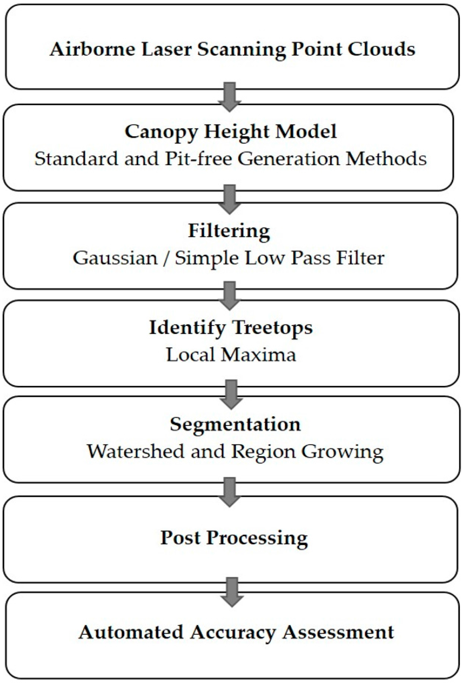
A range of algorithms can be applied for ITC delineation from ALS data, which typically exploit structural differences present among tree tops, canopy boundaries and canopy spaces [14]. These algorithms include the region growing [15,16] and watershed segmentations [14] which often require the prior identification of treetops as seed inputs. From ALS data, treetops are typically located via the detection and filtering of local maxima [17,18], in CHMs these represent points where neighbouring pixels present equal or lower values in height [19]. The performance of a particular ITC delineation algorithm is dependent on the characteristics of both tree canopies and input datasets, and the subsequent suitability of methods for a specific study should be considered [20,21,22].
In the case of ITC delineation, ALS datasets are typically analysed in raster format as a canopy height model (CHM) [23]. A CHM represents the canopy surface elevation and is computed by the subtraction of the digital terrain model (DTM) from the digital surface model (DSM) [24,25]. The selected pixel size for the CHM, can affect the potential performance of the ITC detection [14,26]. In cases where the resolution is too coarse, the ability to distinguish between the boundaries of neighbouring tree crowns can be lost where pixels contain multiple overlapping tree crowns. Conversely, when spatial resolution is too fine, excessive intra-crown height variability may cause an over-segmentation of canopies. Pouliot et al. [20] described the ratio between crown diameter and pixel size in order to address this point. The optimum ratio will vary in accordance with the sensitivity of segmentation algorithms to intra-crown irregularity and the distinction of crown boundaries, but can provide a useful tool in considering the influence of pixel size on ITC delineation success. Nevertheless, the insufficient availability of data regarding the relationship between pixel size and tree crown dimensions makes it difficult to determine specific recommendations for selection [27]. In this paper we will consider the implications of varying CHM pixel size on the performance of ITC delineation across a range of crown dimensions.
Canopy height anomalies that are present in CHMs are known as data pits and can influence the accuracy of ITC detection [25,26]. Despite the uncertainty surrounding the specific source of these pits, cited causal factors have been acknowledged during the acquisition and processing of ALS datasets [25,28], these include: penetration of laser beams through the canopy, merging of ALS flight lines [29], classification of ground and non-ground points [30] and interpolation of point clouds to raster datasets [
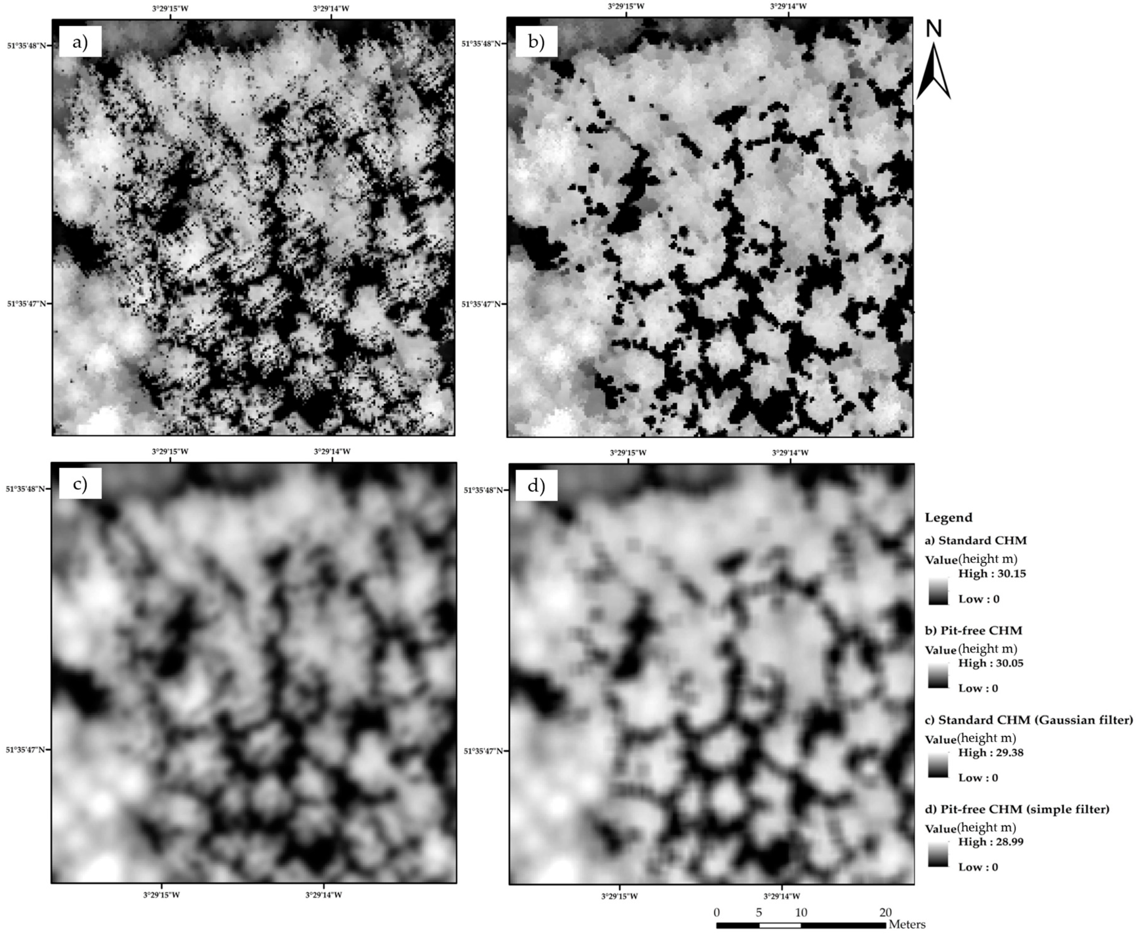
31]. To address the problem, many studies have used image smoothing techniques such as Gaussian filtering, to remove intra-canopy elevation artefacts [12,19,21]. More recent solutions have introduced the use of pit-filling algorithms [25,32] and the application of pit-free CHM generation methodologies [26].
In forests subject to defoliation and dieback as a result of phytopathogens and pests, canopy structures are typically more complex and exhibit larger elevation irregularities across the canopy surface [33,34], causing an increased presence of data pits. Such characteristics can be useful in disease detection [35,36], but may also provide an added complication with regard to the isolation of ITCs for the assessment of crown deterioration. Consequently, the methodologies employed for ITC delineation in canopies affected by disease require consideration of data pits and their implications for segmentation accuracy.
In the case of phytopathological assessments from remotely sensed datasets, the application of an ITC approach presents several advantages for identifying areas that require phytosanitary interventions [37]. In the early stages of the disease establishment in the forest stand, the isolation of ITCs, which initially succumb to infection, can enable a rapid response to pests and pathogens, which present new risks to forest areas [38]. In studies of diseased forest landscapes, crown-based approaches can also facilitate the detailed study of heterogeneous patterns of infection [39]. In addition, the use of ITC delineation techniques alongside species identification [40,41] can facilitate a targeted assessment of susceptible tree species [39]. This combined approach also presents the potential for the identification of disease resistant individuals, which may prove particularly useful with regard to the breeding of resistant genotypes and the development of resilience in forest stock [42]. Resultantly, in the case of P. ramorum, the application of an ITC-based approach could therefore facilitate a detailed assessment of infected forested areas.
To address the difficulties in conducting ITC segmentation in partially or wholly defoliated forest canopies, this study aimed to determine the best method for the extraction of ITCs within P. ramorum infected larch forests using ALS data. In order to identify the most suitable approach the separate influences of segmentation method, CHM resolution and pit-removal were all considered.

2. Materials and Methods

2.1. Study Area

The two study sites are located in Wales, United Kingdom (Figure 1). Ogmore Forest in South Wales (51.595387°N, −3.532012°W) is within the core P. ramorum disease zone in Wales and has been subject to the infection since 2011 [3]. The site contains Japanese larch (Larix kaempferi) and hybrid larch (Larix x eurolepis), two principal host trees of the P. ramorum pathogen [43]. Due to the extent of the P. ramorum infection across the Ogmore study site, plots containing healthy larch could not be established; consequently, a second study site was also used. Radnor Forest in Mid-Wales (52.270817°N, −3.150316°W) was selected as a control site as it is free from the P. ramorum infection. Across the two sites, 8 sample plots were established covering a total area of 0.02 km2 (Table 1). The 4 plots at Ogmore Forest showed a range of P. ramorum infection severities, whilst the 4 plots in Radnor Forest offered healthy trees for comparison across a similar range of species compositions and stand heights. The rectangular plots were situated along the edge of established forest sub-compartments to facilitate access and aid in recording the geographical position of individual trees. Small variations in plot size (Table 1) were incurred as the result of differences in sub-compartment shape and tree crown size.

2.2. Ground Data Collection

The severity of the P. ramorum infection in each plot was recorded during field visits in 2015 using a simple scale:
  • None = no individuals within the plot showed symptoms of P. ramorum;
  • Light = less than 50% of individuals showed P. ramorum symptoms, but these were typically confined to a small portion of the canopy;
  • Moderate = more than 50% of individuals demonstrated P. ramorum symptoms, a few cases may have resulted in significant discolouration or defoliation of the canopy; and
  • Heavy = more than 75% of individuals were infected with P. ramorum and many exhibited severe dieback.
In addition, the position of individual trees situated within the established sample plots, which were safely accessible for ground surveying, were also recorded in the field using a handheld Garmin Oregon 550t GPS.

2.3. Airborne Laser Scanning Data Collection

ALS data were acquired by Bluesky International for both study sites via a single aircraft survey utilising the Orion M300 sensor on the 30 June 2015, with an average flight altitude of 1500 m. The scan frequency was 66 Hz, laser pulse repetition frequency was 100 kHz, field-of-view was 8°, beam divergence was 0.25 mrad, sensor range precision was <8 mm and elevation accuracy was 3–10 cm. Resulting point densities for the Ogmore (infected) and Radnor (control) sites were 20.34 points/m2 and 27.39 points/m2, respectively. Small differences in the resulting point densities across the two sites were incurred as a result of slight variations in flight altitude.

2.4. Data Processing Overview

To provide an overview of the methodology required, Figure 2 provides a summary of the data processing tasks performed.

2.5. Canopy Height Models

CHMs were produced for both study sites using two separate methods. The first approach used a standard normalised digital surface model (CHMstandard) to represent the relative height of above-ground vegetation [19]. Height normalised ALS points were classified into ground and above-ground hits and following the generation of a triangulated irregular network (TIN) were rasterised to produce a DTM (ground points only) and DSM (maximum of all points). Subsequently, the CHMstandard was produced following the subtraction of the DTM from the DSM [44]. In addition, the pit-free algorithm outlined by Khosravipour et al. [26] was also used to generate CHMs for the study areas (CHMpitfree). The method uses height-normalised ALS points for the construction of partial CHMs representing various levels within the canopy (2 m, 5 m, 10 m, 15 m and 20 m). A rasterisation threshold is applied during the triangulation of partial CHMs, to ensure that only triangles within a single crown are rasterised, this threshold was varied based on the pixel size of the CHMs generated (Table 2). Partial CHMs are then stacked in height order and the maximum value for each pixel was subsequently extracted for the creation of the pit-free CHM.
The CHM outputs from both methodologies were generated at three different resolutions. Based on the suitable range of crown diameter to pixel size ratios suggested by Pouliot et al. [20] and the CHM resolutions used in previous ITC detection studies [26,45,46,47], pixel sizes of 0.15 m, 0.25 m and 0.5 m were selected. All the processing for both the CHM approaches was implemented using LAStools [48].

2.6. Manual ITC Delineation

A manual tree crown delineation was performed for each sample plot in order to provide information regarding ITC dimensions and a basis for comparing segmentation results [20]. The manual delineation was performed using the ALS-derived data, in addition to photographs and GPS positions for ITCs recorded during ground surveys [49,50]. The resulting reference polygons enabled the extraction of crown area and diameter. In this case, due to the circular nature of coniferous canopies [50,51], equivalent crown diameter, which represents the diameter of a perfectly circular crown of equal area, was extracted using the diameter equation for a circle [52,53].

2.7. Filtering

The standard CHMs were smoothed with a Gaussian filter to remove data pits and intra-canopy irregularities as shown in Figure 3 [12,19,26,54]. The standard deviation of the Gaussian filter has little impact on the final smoothing of CHMs [14,55] and the standard deviation value was set to 2, following preliminary testing [19]. The size (spatial diameter) of the filter applied, however, can have a significant influence on the resulting CHM. Chen et al. [14] acknowledged that filter size should not exceed that of the smallest crown within the canopy of interest. Subsequently, the filter size was varied for each sample plot in accordance with pre-defined maximum canopy height thresholds (Table 3). These categories were determined based on the minimum equivalent crown diameter and maximum height for each sample plot. The variation in pixel size was also accounted for, with the size of filter in pixels rounded to the closest multiple for each of the three CHM resolutions [56]. For implementation over larger areas of larch forest, it is suggested that filtering and segmentation be employed for individual forest stands using the maximum tree height for each stand to define diameter and tailor filtering to stand characteristics.
In the case of the pit-free CHMs, a low-pass smoothing filter was applied (Figure 3). Preliminary testing was carried out to consider the performance of the pit-free CHMs without smoothing, however in the majority of cases the reduction in intra-canopy variation as a result of the filter prevented the over-segmentation of ITCs. Due to the removal of data pits via the CHM generation methodology, a lower level of filtering was required to smooth the canopy surface in preparation for segmentation. In this case a simple low-pass smoothing filter was selected with a square search mode [20,22]. The filter size was also adjusted in accordance with maximum tree height (Table 4), however it was smaller than that applied for the CHMstandard, which over-smoothed the data. All filtering undertaken for both CHM generation methodologies was undertaken using SAGA GIS [57].

2.8. Local Maxima

Prior to the application of the selected segmentation methods (marker-controlled watershed and region growing algorithm), seed points representing treetops within the canopy need to be identified [16,58]. Treetops can be located via the identification of local maxima [59], which are detected when neighbouring pixels on the CHM exhibit equal or lower height values [19]. In order to avoid identifying multiple seed points within ITCs, local maxima were extracted from the smoothed standard and pit-free CHMs for each of the three resolutions [14]. Resulting local maxima were then subject to height filtering, removing points with a tree height of less than 2 m, to avoid the detection of understorey vegetation as tree crowns [54,60].
In addition, minimum distance filters can also be applied to local maxima to reduce the over-estimation of the number of treetops. The size of these filters can be fixed or variable; however, their dimensions are typically informed by the diameter of tree crowns within the forest area of study. Variable filters are typically applied with regard to the relationship between tree height and crown diameter [14], which in this instance exhibits high levels of variation (Figure 4). A weak relationship between crown diameter and tree height can result in poor estimates of tree crown diameter [61]. To detect treetops with smaller crowns, filter size thresholds were used [19]. As with the Gaussian smoothing, filter diameter represented the minimum equivalent crown diameter in relation to the maximum tree height for the sample plots (Table 3). This minimal distance point filtering was applied to local maxima points for each sample plot following height filtering, and all processing was performed in SAGA GIS [57].

2.9. Segmentation

For CHMs, the marker-controlled watershed and region growing segmentation algorithms have both previously been acknowledged as effective approaches for the delineation of ITCs [14,62]. The marker-controlled watershed algorithm treats the inverted CHM as “valleys”, “flooding” each system from points of local minima (markers or seeds) representing treetops within the canopy. Respective boundaries for each tree crown are subsequently delineated by determining the “watershed” for each individual “valley” [58]. The region growing algorithm also requires a seed input to denote the location of treetops, from which neighbouring pixels are compared and merged until some specified threshold criteria is reached [16,27,63]. In the case of both segmentation methods, filtered local maxima were used as seed inputs and processing was undertaken in SAGA GIS [63,64,65,66,67]. Additional input parameters for the two segmentation algorithms in SAGA GIS [57] were subject to preliminary testing. Subsequently the marker-controlled watershed segmentation was subject to no additional threshold for joining segments. For the region growing segmentation, the similarity threshold was set to 0.01 and an 8-pixel neighbourhood was applied.

2.10. Post-Processing

Following the ITC delineations, output segments from both segmentation approaches were labelled with a unique ID [68], converted to polygons and joined with tree heights extracted from seed outputs [69]. To avoid over-segmentation, polygons with an area below that of the minimum threshold area (Table 5) derived as the circular area from the Gaussian and local maxima filter size diameters, were merged with the neighbouring segment exhibiting the longest common border [19,70].

2.11. Accuracy Assessment

To assess the accuracy of the automated ITC delineations, resulting segments were compared to manual tree crown delineations (reference crowns) via an automated overlap analysis, which determined the percentage of overlap for corresponding polygons. For each reference crown in the plot, the percentage overlap with automated polygons was computed. Subsequently, the two highest percentage overlap values for individual reference crowns were recorded as R1 and R2. In addition, the percentage of the automated polygons which overlapped with the corresponding reference crown were also determined, the two highest values were reported as A1 and A2. Using these values for each reference tree, percentage overlap criteria were subsequently applied to previously established accuracy assessment categories (Table 6) [17,19,23,29,50,71]. ITC segmentations classified as correct or satisfactory were deemed acceptable for the purpose of the study and collectively referred to as successfully delineated segments [17,71]. Accuracy percentages were also calculated using the ratio of successful delineations to the total number of reference tree crowns for each plot [23].

2.12. Data Analysis

To evaluate the influence of CHM generation method on delineation accuracy, the non-parametric Wilcoxon signed rank test was used to analyse the difference in the segmentation accuracy percentages produced by the standard and pit-free CHMs for each of the pixel size/segmentation algorithm combinations. The same testing was also applied in the comparison of two segmentation algorithms (marker-controlled watershed and region growing), for each of the CHM generation method/pixel size combinations. The equivalent parametric paired t-test was not selected in this instance as several datasets did not meet the assumptions of normality (Shapiro–Wilk test). To address the additional type 1 error incurred via multiple testing, the Holm–Bonferroni sequential correction was also applied to the results of the statistical testing.
To consider the influence of CHM pixel size on delineation accuracy, the mean and standard deviation values for segmentation accuracy percentages across all study plots were calculated for each CHM generation method/segmentation algorithm combination. In addition, to assess the relationship between CHM pixel size and tree height, a linear regression model was fitted to the maximum plot tree height (m) and the percentage of successful delineation (%), for all segmentation algorithms and CHMs tested.

3. Results

3.1. Overall Segmentation Performance

The ITC delineation results from the marker-controlled watershed and region growing segmentations for all CHMs are displayed in Table 7, with the highest percentages for each of the plots in bold. In cases where the highest percentage is tied, those producing the greater percentage of correct delineations (Table 6) were selected. Successful delineations exceeding 70% were achieved for all of the sample areas, however no single method or CHM presented optimal results across all sample plots. The most successful delineation method recorded for each of the sample plots is summarised in Table 8.

3.2. CHM Generation Method

Table 8 shows which CHM generation method produced the most successful delineation accuracies. The standard and pit-free methodologies both performed best in four of the eight sample plots. Interestingly, for Plots 2, 3 and 4, which exhibited moderate and heavy severities of P. ramorum infection, the pit-free CHM generated the best delineation accuracies. Figure 5 displays the difference in successful delineation percentages for the standard and pit-free CHMs, across the three different pixel sizes tested. In the case of the 0.15 m pixel size, the standard CHM produced the best accuracies for all segmentations across the eight sample plots, except one (Plot 6, region growing, 0.15 m). Conversely, for the 0.5 m pixel size, the pit-free CHM generation method resulted in a more successful delineation for the majority of segmentations. At the 0.25 m pixel size however, the CHM generation methods performed similarly. The segmentation algorithms did not influence the success of the two CHM generation methods. The results from the statistical analysis (Table 9) demonstrate no significant difference between the delineation accuracy of the two different CHM generation methods, except in the case of the marker-controlled watershed segmentation at the 0.15 m pixel size (p > 0.10).

3.3. Segmentation Algorithim

The marker-controlled watershed approach produced higher delineation accuracies across the sample plots, than the region growing method (Figure 6). This result was consistent across the two CHM generation methodologies and three pixel sizes tested. The greatest difference (73.69) was observed in the case of the CHMstandard in at the 0.5 m pixel size. In this instance 71% of tree crowns segmented with the region growing algorithm were categorised as missed (Table 6). The results from the Wilcoxon signed rank test (Table 10) indicated a significant difference, at the 90% confidence level (p < 0.10) between the segmentation algorithms across all CHM generation method/pixel size combinations tested.

3.4. CHM Pixel Size

In relation to CHM pixel size, no single resolution consistently yielded the most successful delineations (Table 8). To consider the overall performance of each pixel size, Table 11 provides the mean and standard deviation values for the successful delineation percentages from all eight sample plots, for each of the segmentation algorithm and CHM generation methodology combinations tested. The 0.25 m resolution provided the highest mean value in three of the four instances. Additionally, the 0.25 m pixel size also exhibited comparatively low standard deviation values in the case of the two marker-controlled watershed segmentations. The higher standard deviations across all combinations at the 0.15 m and 0.5 m resolutions, in addition to the 0.25 m region growing segmentations, reflect the large disparities in successful delineations percentages across the eight sample plots.
The segmentation results suggest that the suitability of CHM pixel size for ITC delineation may be governed by crown size and tree height, two correlated variables regarding the structural character of individual trees. Figure 7 presents the relationship between tree height and segmentation accuracy for all of the segmentation algorithms and CHMs tested. The linear regressions suggest that the high-resolution CHMs (0.15 m) performed best for plots with a low maximum tree height (<20 m). Conversely, the lowest resolution CHM (0.5 m) was best suited for plots that exhibited a high maximum tree height (>30 m). In the case of the 0.25 m pixel size, the relationship between maximum tree height and successful delineation percentage is less clear, although a negative trend was typically observed.
Each of the scatterplots in Figure 7 displays the R2 values for the fit of the linear regression model between maximum tree height per plot (m) and successful delineation (%), at the three CHM pixel sizes (0.15 m, 0.25 m and 0.5 m) for the different segmentation algorithms and CHM generation methods. For the 0.15 m pixel size, negative trends were consistent across the two segmentation algorithms and CHM generation methods, though more significant in the case of the region growing segmentations (0.82 (standard) and 0.78 (pit-free)). At the 0.25 m pixel size, trends were predominantly negative and stronger for segmentations with the region growing algorithm (0.86 (standard) and 0.64 (pit-free)). In contrast, segmentations at the 0.5 m pixel size typically exhibited a positive relationship between maximum plot tree height and success percentage, with stronger correlations produced by the marker-controlled watershed segmentations (0.73 (standard) and 0.86 (pit-free).
An additional approach to examine the relationship between pixel size and successful ITC delineation considered the crown diameter to pixel size ratio put forward by Pouliot et al. [20]. For each sample plot, the mean equivalent crown diameter was determined in order to produce the crown diameter to pixel ratios for each of the eight sample plots (Table 12). The ratios that contributed to the best performance for each of the plots ranged between 10:1 and 35:1. To consider the influence of these ratios on the performance of ITC segmentations, the relationship between the mean equivalent crown diameter to pixel size ratio and successful delineations (%) across all sample plots, segmentation approaches and CHMs is shown in Figure 8. Segmentations that exceeded 80% success rate exhibited a crown diameter to pixel ratio from 11:1 to 35:1.

4. Discussion

The absence of an optimal method or input CHM for ITC delineation across the study plots highlights the difficulties of utilising a single algorithm and input dataset to assess forest environments comprising of mixed stand ages and species [12,47]. Nevertheless, the results shown here allow us to infer several key points informing the selection of the most appropriate segmentation approach and CHM input for canopies subject to P. ramorum infection.
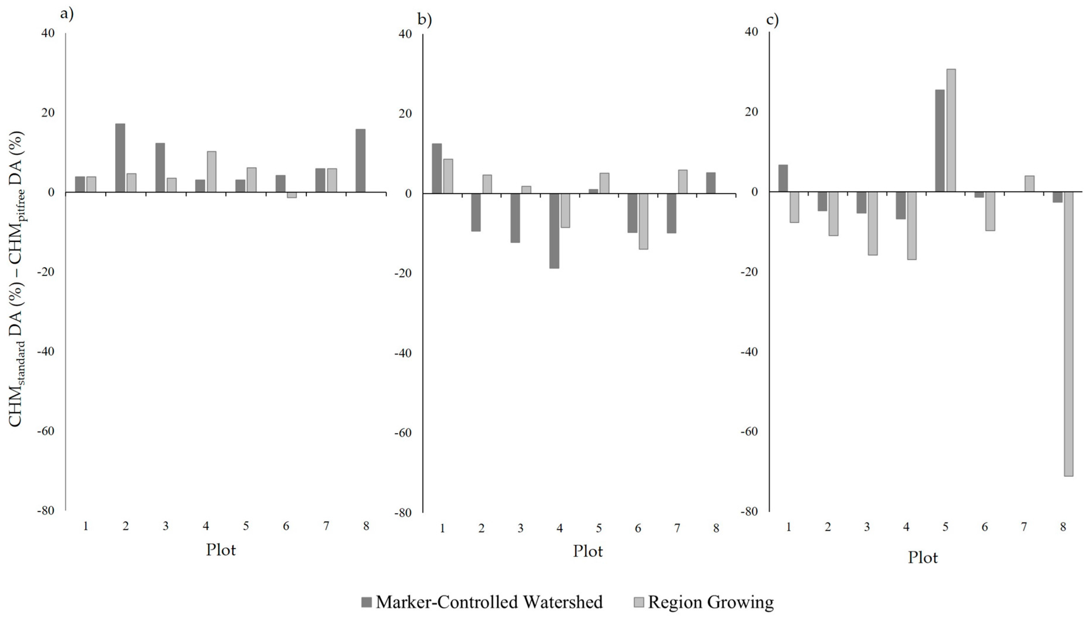
Neither CHM generation method (standard/pit-free) exhibited a consistently stronger performance, with each outperforming the other for four of the eight sample plots. This is different from the results observed by Khosravipour et al. [26], who documented consistently improved tree top detection accuracy for all pit-free CHM inputs at pixel sizes of 0.15 m and 0.5 m. In our case, it is likely that the weaker performance of the pit-free CHMs in four of the sample plots may stem from the low-pass filtering used to smooth the canopy surface for improved local maxima detection. This was not applied in the study by Khosravipour et al. [26], who instead extracted local maxima with an established variable window for coniferous forests [51]. In addition, Khosravipour et al. [26] assessed the accuracy of treetop detection, rather than the segmentation on ITCs. Nevertheless, in the case of the Plots 2, 3 and 4 which were subject to moderate and heavy 
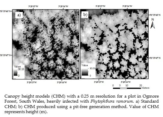
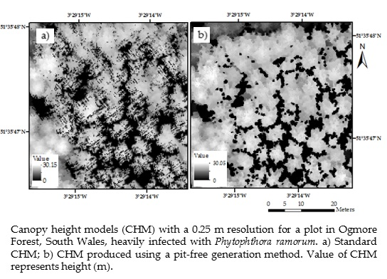
P. ramorum infection, the pit-free CHMs out performed those generated using the standard CHM. This improved performance is likely to be a result of the data pit filling during the CHM generation, providing a more complete canopy for image segmentation (Figure 3).
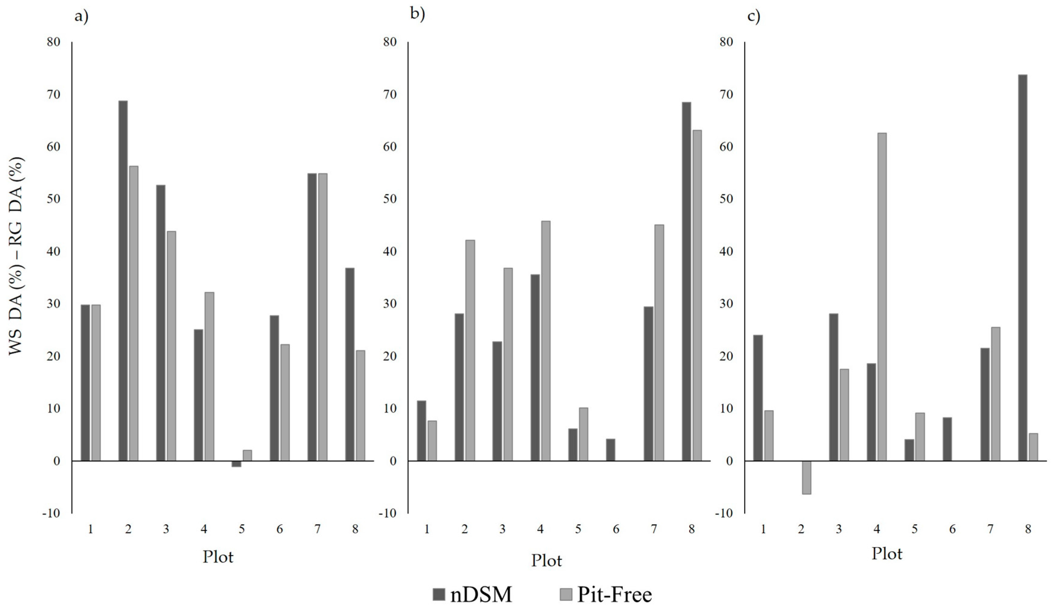
Between the two segmentation algorithms, the marker-controlled watershed demonstrated a superior performance (p < 0.10) compared to the region growing segmentation, for both CHM generation methods and all CHM pixel sizes tested. Since both algorithms were provided with the same seed points, the difference in performance is due to their ability to delineate crown boundaries in the CHMs. In the case of the region growing segmentation, boundaries are delineated when a specified threshold value is reached. The poor overall performance of this particular segmentation algorithm is likely to have resulted from the inability of the region growing threshold to accommodate the variation in crown size and characteristics across the canopy, as a result of mixed species and tree ages [50]. Although the region growing algorithm has previously produced satisfactory ITC delineations [27,72,73,74], studies have also noted difficulties and poor performance associated with the algorithm when applied in forest stands comprising of mixed species, multiple canopy layers and high tree densities [27,73,74]. In comparison, the delineation of crown boundaries by the watershed segmentation directly utilises the height information for the CHMs when delineating watershed boundaries, providing a more informed segmentation [58]. Studies from an array of forest types have noted successful isolation or segmentation of ITCs resulting from the marker-controlled watershed segmentation, examples include: commercially thinned conifer forest (75.6%) [58], savanna woodland (64.1%) [14] and eucalypts forest [75]. Nevertheless, the delineation accuracies achieved by segmentation algorithms can vary due to a combination of factors including: the effectiveness of the algorithm, forest characteristics and ALS data acquisition and properties [65]. Consequently, the difference between the performance of the marker-controlled watershed and region growing algorithms may change for segmentations performed for other forest environments and ALS datasets.
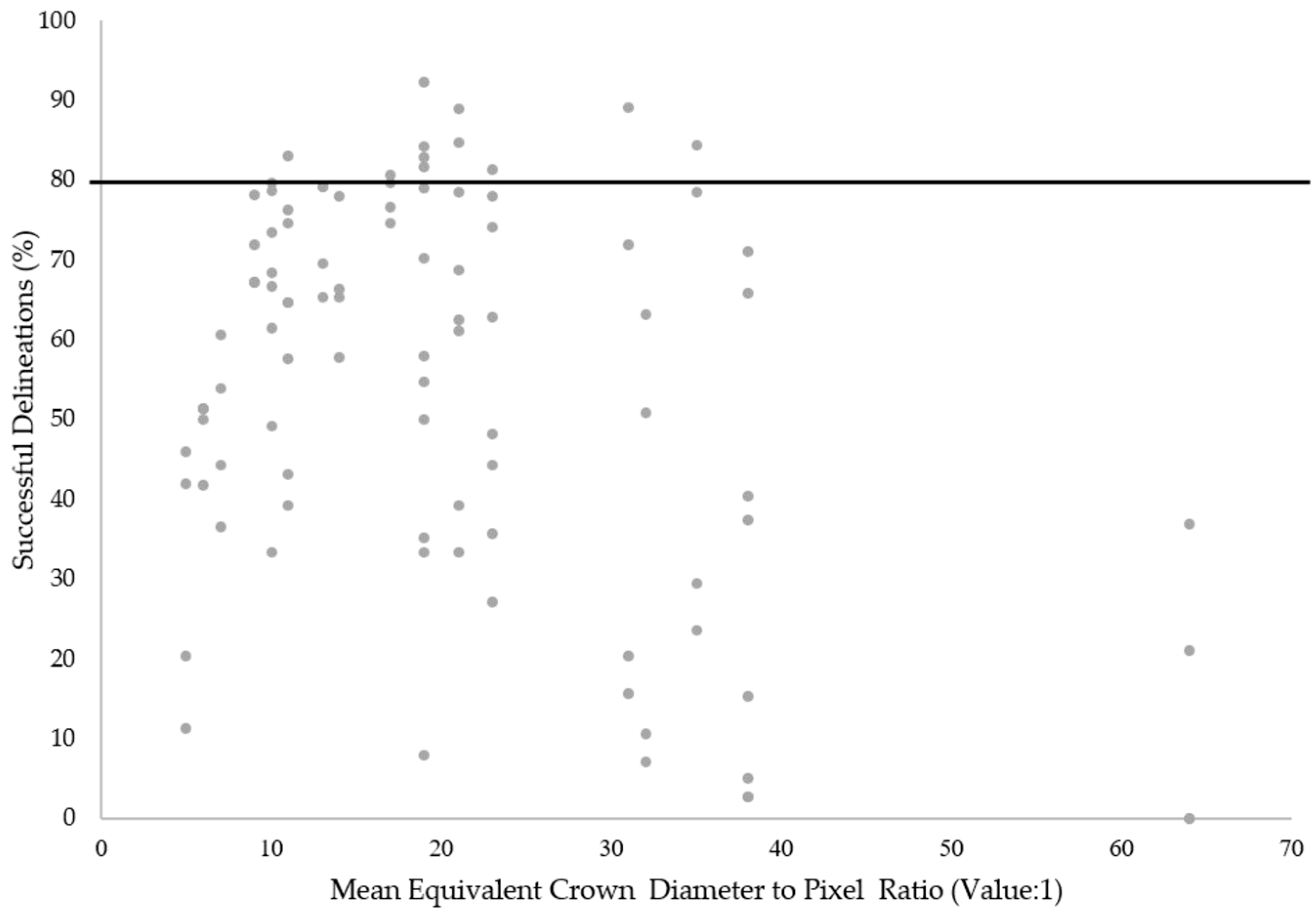
The results from the study also highlighted that CHM resolution used in the ITC segmentation strongly influences segmentation accuracy. Relationships between the maximum canopy height and optimum CHM pixel size were not unexpected given the strong influence of tree height on crown diameter [14]. The suitability of certain pixel sizes for particular forest canopies has previously been explored in the literature [20]. For example, with regard to crown diameter to pixel ratios, Pouliot et al. [20] suggested a lower and upper limit of 3:1 and 19:1 respectively. In comparison, the ratios (mean equivalent crown diameter) that produced the best tree crown delineations across the sample plots were slightly higher, between 10:1 and 35:1. This may be as a result of reduced intra-canopy variation within the CHMs caused by the image smoothing filters applied [12,19]. In addition, these examples from Pouliot et al. [20] were also suggested for imagery rather than CHMs produced from ALS. Previous studies have also considered the impact of CHM resolution on segmentation accuracy, Stereńczak et al. [76] for example, noted no significant difference between the ITC segmentation results from the 0.25 m and 0.5 m resolution CHMs, however a significant reduction in the percentage of recognised ITCs was noted for the 1.0 m CHM. The results from previous research, in addition to those obtained in this study highlight the importance of selecting a suitable CHM pixel size for ITC segmentation. Nevertheless, in many cases the selected resolution of the CHMs utilised for ITC segmentations is governed by ALS point density [26].
In relation to each of the CHM resolutions, several observed relationships require further discussion. Firstly, the 0.25 m CHM resolution performed consistently well across all sample plots, especially for the marker-controlled watershed segmentations, suggesting that this pixel size may be most suitable for the two study areas as a whole. This implies that at the 0.25 m resolution, enough detail is provided for the majority of ITCs to delineate boundaries without high levels intra-canopy variation resulting in over segmentations. However, in the cases of plots which exhibited a large maximum tree height (>30 m), the application of a lower resolution CHM (0.5 m) typically facilitated a greater percentage of successful ITC delineations. Again, the level of intra-crown variation provided in the CHM is likely to be the causal factor for this observation. With regard to the higher resolution CHMs (0.15 m) tested, a relationship between pixel size suitability and maximum tree height was also evident. In this instance, plots characterised by a small maximum tree height (<20 m) in general produced higher percentages of successful ITC delineations.
Nevertheless, it is important to note, that while these criteria explain the characteristic relationship between pixel size, maximum tree height and successful ITC delineation across the sample plots, variability in the observed trend was also evident in the dataset. This suggests that other plot characteristics such as variation in tree size and tree density may also influence the suitability of a particular CHM pixel size for ITC segmentation [50]. Hence, it should be acknowledged that, while crown diameter should be recognised as a dominant variable influencing the suitability of pixel sizes for ITC delineation, consideration should also be given to other forest characteristics. In addition, it should also be recognised that the level of intra-canopy variation is also controlled by the filtering of the CHMs before segmentation [14]. Consequently, relationships between the performance of CHMs at different resolutions and tree height may be altered for CHMs subject to varying degrees of smoothing.
The research demonstrates that ITCs within larch stands affected by P. ramorum can be successfully delineated (>70%) using a pit-free CHM generation methodology, a marker-controlled watershed segmentation and the selection of an appropriate CHM pixel size. Nevertheless, whilst these methods provide successful results at the selected study sites, further testing would be required to consider the performance these methods for defoliated canopies of other tree species in different forest environments. In addition, preliminary testing was used to identify the most suitable parameters in the filtering and segmentation processes, however such parameters can significantly influence final segmentation results and may not be best suited for other forest environments and ALS datasets [14,72]. Furthermore, an additional limitation to the study can also be noted with regard to the use of two separate study areas for the comparison between healthy and infected stands. Although larch dominated plots were selected to best match with regard to tree height parameters, variations in tree density and species composition may have also influenced the performance of ITC segmentations across the two sites.

5. Conclusions

The results presented in the study highlight that larch canopies partially or wholly defoliated as a result of P. ramorum infection can be successfully segmented (>70%). In addition, the research also demonstrates that the selection of segmentation algorithm, CHM generation method and CHM resolution can all impact on the performance of ITC delineations from ALS for larch forests in the U.K. The marker-controlled watershed algorithm may provide better successful delineations percentages in comparison to the region growing method in mixed age plantation forests (p < 0.10), where the selected threshold value may limit the optimal application of the segmentation across all crowns. In the case of forests subject to moderate and severe defoliation due to P. ramorum infection, the application of a pit-free CHM generation method facilitated a greater ITC delineation percentage than segmentations using a standard CHM. With regard to CHM resolution, the results from the research suggest that a 0.25 m pixel size was most suitable for the larch dominated plots of all ages. In the case of the plots which exhibited large (>30 m) or small (<20 m) maximum tree heights, the selection of lower (0.5 m) or higher (0.15 m) resolution CHM, respectively, provided a more successful delineation. Overall, the results demonstrate that despite the increased presence of data pits in defoliated canopies, ITCs subject to infection from phytopathogens can be successfully identified. Whilst the presented methods provide a benchmark for the segmentation of ITCs subject to decline from phytopathogens, in order to consider the performance of this approach in other defoliated tree species and environments further research would be required.

Acknowledgments

The work was funded as part of a NERC CASE studentship with partner Bluesky International. Natural Resources Wales were also a key partner to the research providing expertise, support and access to study sites. Forest Inventory GIS datasets (Ogmore and Radnor Forest) from the Forestry Commission were also accessed to provide data regarding the two field sites.

Author Contributions

All authors conceived and designed the experiments; Chloe Barnes performed the experiments and analysed the data; all authors contributed reagents/materials/analysis tools; and Chloe Barnes, Heiko Balzter and Kirsten Barrett wrote the paper.

Conflicts of Interest

The authors declare no conflict of interest.

References

  1. Sutherland, W.J.; Bailey, M.J.; Bainbridge, I.P.; Brereton, T.; Dick, J.T.A.; Drewitt, J.; Dulvy, N.K.; Dusic, N.R.; Freckleton, R.P.; Gatson, K.J.; et al. Future novel threats and opportunities facing UK biodiversity identified by horizon scanning. J. Appl. Ecol. 2008, 45, 821–833. [Google Scholar] [CrossRef]
  2. Potter, C.; Harwood, T.; Knight, J.; Tomlinson, I. Learning from history, predicting the future: The UK Dutch elm disease outbreak in relation to contemporary tree disease threats. Philos. Trans. R. Soc. B Biol. Sci. 2011, 366, 1966–1974. [Google Scholar] [CrossRef] [PubMed]
  3. Forestry Commission. Phytophthora ramorum outbreak and risk zones maps. Available online: http://www.forestry.gov.uk/forestry (accessed on 11 March 2016).
  4. Webber, J.F.; Mullett, M.; Brasier, C.M. Dieback and mortality of plantation Japanese larch (Larix kaempferi) associated with infection by Phytophthora ramorum. New Dis. Rep. 2010, 22, 19. [Google Scholar] [CrossRef]
  5. Medcalf, K.A.; Bodevin, N.; Cameron, I.; Webber, J.; Turton, N. Assessing the Potential of Using Remote Sensing in Support of Current Phytophthora Work. Available online: http://www.envsys.co.uk/wp-content/uploads/2015/02/Remote_Sensing_Phytophthora.pdf (accessed on 8 March 2016).
  6. Lefsky, M.A.; Cohen, W.B.; Acker, S.A.; Parker, G.G.; Spies, T.A.; Harding, D. Lidar remote sensing of the canopy structure and biophysical properties of Douglas-fir western hemlock forests. Remote Sens. Environ. 1999, 70, 339–361. [Google Scholar] [CrossRef]
  7. Lim, K.; Treitz, P.; Wulder, M.; St-Onge, B.; Flood, M. LiDAR remote sensing of forest structure. Prog. Phys. Geogr. 2003, 27, 88–106. [Google Scholar] [CrossRef]
  8. Wulder, M.A.; Coops, N.C.; Hudak, A.T.; Morsdorf, F.; Nelson, R.; Newnham, G.; Vastaranta, M. Status and prospects for LiDAR remote sensing of forested ecosystems. Can. J. Remote Sens. 2006, 39, S1–S5. [Google Scholar] [CrossRef]
  9. Popescu, S.C.; Wynne, R.H.; Nelson, R.F. Measuring individual tree crown diameter with lidar and assessing its influence on estimating forest volume and biomass. Can. J. Remote Sens. 2003, 29, 564–577. [Google Scholar] [CrossRef]
  10. Zimble, D.A.; Evans, D.L.; Carlson, G.C.; Parker, R.C.; Grado, S.C.; Gerard, P.D. Characterizing vertical forest structure using small-footprint airborne LiDAR. Remote Sens. Environ. 2003, 87, 171–182. [Google Scholar] [CrossRef]
  11. Balzter, H.; Luckman, A.; Skinner, L.; Rowland, C.; Dawson, T. Observations of forest stand top height and mean height from interferometric SAR and LiDAR over a conifer plantation at Thetford Forest, UK. Int. J. Remote Sens. 2007, 28, 1173–1197. [Google Scholar] [CrossRef]
  12. Brandtberg, T.; Warner, T.A.; Landenberger, R.E.; McGraw, J.B. Detection and analysis of individual leaf-off tree crowns in small footprint, high sampling density lidar data from the eastern deciduous forest in North America. Remote Sens. Environ. 2003, 85, 290–303. [Google Scholar] [CrossRef]
  13. Reutebuch, S.E.; Andersen, H.E.; McGaughey, R.J. Light detection and ranging (LiDAR): An emerging tool for multiple resource inventory. J. For. 2005, 103, 286–292. [Google Scholar]
  14. Chen, Q.; Baldocchi, D.; Gong, P.; Kelly, M. Isolating individual trees in a savanna woodland using small footprint lidar data. Photogramm. Eng. Remote Sens. 2006, 72, 923–932. [Google Scholar] [CrossRef]
  15. Erikson, M. Segmentation of individual tree crowns in colour aerial photographs using region growing supported by fuzzy rules. Can. J. For. Res. 2003, 33, 1557–1563. [Google Scholar] [CrossRef]
  16. Tiede, D.; Hochleitner, G.; Blaschke, T. A full GIS-based workflow for tree identification and tree crown delineation using Laser scanning. In Proceedings of the ISPRS Workshop (CMRT 05), Vienna, Austria, 29–30 August 2005; pp. 9–14.
  17. Kwak, D.A.; Lee, W.K.; Lee, J.H.; Biging, G.S.; Gong, P. Detection of individual trees and estimation of tree height using LIDAR data. J. For. Res. 2007, 12, 425–434. [Google Scholar] [CrossRef]
  18. Zhen, Z.; Quackenbush, L.J.; Zhang, L. Impact of tree-orientated growth order in marker-controlled region growing for individual tree crown delineation using airborne laser scanner (ALS) data. Remote Sens. 2014, 34, 4636–4654. [Google Scholar]
  19. Koch, B.; Heyder, U.; Weinacker, H. Detection of individual tree crowns in airborne LiDAR data. Photogramm. Eng. Remote Sens. 2006, 72, 357–363. [Google Scholar] [CrossRef]
  20. Pouliot, D.A.; King, D.J.; Bell, F.W.; Pitt, D.G. Automated tree crown detection and delineation in high-resolution digital camera imagery of coniferous forest regeneration. Remote Sens. Environ. 2002, 82, 322–324. [Google Scholar] [CrossRef]
  21. Jing, L.; Hu, B.; Li, J.; Noland, T. Automated delineation of individual tree crowns from LiDAR data by multi-scale analysis and segmentation. Photogramm. Eng. Remote Sens. 2012, 78, 1275–1284. [Google Scholar] [CrossRef]
  22. Kaartinen, H.; Hyyppä, J.; Yu, X.; Vastaranta, M.; Hyyppä, H.; Kukko, A.; Holopainen, M.; Heipke, C.; Hirschmugl, M.; Morsdorf, F.; et al. An international comparison of individual tree detection and extraction using airborne laser scanning. Remote Sens. 2012, 4, 950–974. [Google Scholar] [CrossRef] [Green Version]
  23. Hu, B.; Li, J.; Jing, L.; Judah, A. Improving the efficiency and accuracy of individual tree crown delineation from high-density LiDAR data. Int. J. Appl. Earth Obs. Geoinf. 2014, 26, 145–155. [Google Scholar] [CrossRef]
  24. Dubayah, R.O.; Drake, J.B. Lidar remote sensing for forestry. J. For. 2000, 98, 44–46. [Google Scholar]
  25. Ben-Arie, J.R.; Hay, G.J.; Powers, R.P.; Castilla, G.; St-Onge, B. Development of a pit filling algorithm for LiDAR canopy height models. Comput. Geosci. 2009, 35, 1940–1949. [Google Scholar] [CrossRef]
  26. Khosravipour, A.; Skidmore, A.K.; Isenburg, M.; Wang, T.; Hussin, Y.A. Generating pit-free canopy height models from airborne lidar. Photogramm. Eng. Remote Sens. 2014, 80, 863–872. [Google Scholar] [CrossRef]
  27. Ke, Y.; Quackenbush, L.J. A review of methods for automatic individual tree-crown detection and delineation from passive remote sensing. Int. J. Remote Sens. 2011, 32, 4725–4747. [Google Scholar] [CrossRef]
  28. Véga, C.; Durrieu, S. Multi-level filtering segmentation to measure individual tree parameters based on lidar data: Application to a mountainous forest with heterogeneous stands. Int. J. Appl. Earth Obs. Geoinf. 2011, 13, 646–656. [Google Scholar] [CrossRef] [Green Version]
  29. Leckie, D.; Gougeon, F.; Hill, D.; Quinn, R.; Armstrong, L.; Shreenan, R. Combined high-density lidar and multispectral imagery for individual tree crown analysis. Can. J. For. Res. 2003, 29, 633–649. [Google Scholar] [CrossRef]
  30. Kraus, K.; Pfeifer, N. Determination of terrain models in wooded areas with airborne laser scanner data. ISPRS J. Photogramm. Remote Sens. 1998, 53, 193–203. [Google Scholar] [CrossRef]
  31. Axelsson, P. Processing of laser scanner data—Algorithms and applications. ISPRS J. Photogramm. Remote Sens. 1999, 54, 138–147. [Google Scholar] [CrossRef]
  32. Zhao, D.; Pang, Y.; Li, Z.; Sun, G. Filling invalid values in a LiDAR-derived canopy height model with morphological crown control. Int. J. Remote Sens. 2013, 34, 4636–4654. [Google Scholar] [CrossRef]
  33. Holdenrieder, O.; Pautasso, M.; Weisberg, P.J.; Lonsdale, D. Tree diseases and landscape processes: the challenge of landscape pathology. TRENDS Ecol. Evol. 2004, 19, 446–452. [Google Scholar] [CrossRef] [PubMed]
  34. Larsen, M.; Eriksson, M.; Descombes, X.; Perrin, G.; Brandtberg, T.; Gougeon, F.A. Comparison of six individual tree crown detection algorithms evaluated under varying forest conditions. Int. J. Remote Sens. 2011, 32, 5827–5852. [Google Scholar] [CrossRef]
  35. Coops, N.C.; Varhola, A.; Bater, C.W.; Teti, P.; Boon, S.; Goodwin, N.; Weiler, M. Assessing differences in tree and stand structure following beetle infestation using lidar data. Can. J. Remote Sens. 2009, 35, 497–508. [Google Scholar] [CrossRef]
  36. Bright, B.C.; Hudak, A.T.; McGaughey, R.; Andersen, H.E.; Negrón, J. Predicting live and dead tree basal area of bark beetle affected forests from discrete-return lidar. Can. J. Remote Sens. 2013, 39, S99–S111. [Google Scholar] [CrossRef]
  37. Leckie, D.G.; Walsworth, N.; Gougeon, F.A. Identifying tree crown delineation shapes and need for remediation on high resolution imagery using an evidence based approach. ISPRS J. Photogramm. Remote Sens. 2016, 114, 206–227. [Google Scholar] [CrossRef]
  38. Wulder, M.A.; Dymond, C.C.; White, J.C.; Leckie, D.G.; Carroll, A.L. Surveying mountain pine beetle damage of forests: A review of remote sensing opportunities. For. Ecol. Manag. 2006, 221, 27–41. [Google Scholar] [CrossRef]
  39. Stone, C.; Coops, N.C. Assessment and monitoring of damage from insects in Australian eucalypt forests and commercial plantations. Aust. J. Entomol. 2004, 43, 283–292. [Google Scholar] [CrossRef]
  40. Persson, Å.; Holmgren, J.; Söderman, U.; Olsson, H. Tree species classification of individual trees in Sweden by combining high resolution laser data with high resolution near-infrared digital images. Int. Arch. Photogramm. Remote Sens. Spat. Inf. Sci. 2004, 36, 204–207. [Google Scholar]
  41. Li, J.; Hu, B.; Noland, T.L. Classification of tree species based on structural features derived from high density LiDAR data. Agric. For. Meteorol. 2013, 171, 104–114. [Google Scholar] [CrossRef]
  42. Sniezko, R.A. Resistant breeding against nonnative pathogens in forest trees—Current successes in North America. Can. J. Plant Pathol. 2006, 28, S270–S279. [Google Scholar] [CrossRef]
  43. Brasier, C.; Webber, J. Plant pathology: sudden larch death. Nature 2010, 466, 824–825. [Google Scholar] [CrossRef] [PubMed]
  44. Jakubowski, M.K.; Li, W.; Guo, Q.; Kelly, M. Delineating individual trees from LiDAR data: A comparison of vector-and raster-based segmentation approaches. Remote Sens. 2013, 5, 4163–4186. [Google Scholar] [CrossRef]
  45. Pitkänen, J.; Maltamo, M.; Hyyppä, J.; Yu, X. Adaptive methods for individual tree detection on airborne laser based canopy height model. Int. Arch. Photogramm. Remote Sens. Spat. Inf. Sci. 2004, 36, 187–191. [Google Scholar]
  46. Roberts, S.D.; Dean, T.J.; Evans, D.L.; McCombs, J.W.; Harrington, R.L.; Glass, P.A. Estimating individual tree leaf area in loblolly pine plantations using LiDAR-derived measurements of height and crown dimensions. For. Ecol. Manag. 2005, 213, 54–70. [Google Scholar] [CrossRef]
  47. Solberg, S.; Naesset, E.; Bollandas, O.M. Single tree segmentation using airborne laser scanner data in a structurally heterogeneous spruce forest. Photogramm. Eng. Remote Sens. 2006, 72, 1369–1378. [Google Scholar] [CrossRef]
  48. LAStools. Available online: https://rapidlasso.com/lastools (accessed on 1 June 2016).
  49. Brandtberg, T.; Walter, F. Automated delineation of individual tree crowns in high spatial resolution aerial images by multiple-scale analysis. Mach. Vis. Appl. 1998, 11, 64–73. [Google Scholar] [CrossRef]
  50. Fang, F.; Im, J.; Lee, J.; Kim, K. An improved tree crown delineation method based on live crown ratios from airborne LiDAR data. GISci. Remote Sens. 2016, 53, 402–419. [Google Scholar] [CrossRef]
  51. Popescu, S.C.; Wynne, R.H. Seeing the trees in the forest: Using lidar and multispectral data fusion with local filtering and variable window size for estimating tree height. Photogramm. Eng. Remote Sens. 2004, 70, 589–604. [Google Scholar] [CrossRef]
  52. Persson, Å.; Holmgren, J.; Söderman, U. Detecting and measuring individual trees using an airborne laser scanner. Photogramm. Eng. Remote Sens. 2002, 68, 1313–1323. [Google Scholar]
  53. Morsdorf, F.; Meier, E.; Kötz, B.; Itten, K.I.; Dobbertin, M.; Allgöwer, B. LiDAR-based geometric reconstruction of boreal type forest stands at single tree level for forest and wildland fire management. Remote Sens. Environ. 2004, 92, 353–363. [Google Scholar] [CrossRef]
  54. Hyyppä, J.; Yu, X.; Hyyppä, H.; Vastaranta, M.; Holopainen, M.; Kukko, A.; Kaartinen, H.; Jaakkola, A.; Vaaja, M.; Koskinen, J.; et al. Advances in forest inventory using airborne laser scanning. Remote Sens. 2012, 4, 145–155. [Google Scholar] [CrossRef]
  55. Dralle, K.; Rudemo, M. Stem number estimation by kernel smoothing of aerial photos. Can. J. For. Res. 1996, 26, 1228–1236. [Google Scholar] [CrossRef]
  56. Monnet, J.M.; Mermin, E.; Chanussot, J.; Berger, F. Tree top detection using local maxima filtering: A parameter sensitivity analysis. In Proceedings of the 10th International Conference on LiDAR Applications for Assessing Forest Ecosystems (Silvilaser 2010), Freiburg, Germany, 14–17 September 2010; p. 9.
  57. SAGA GIS. System for Automated Geoscientific Analyses. Available online: http://www.saga-gis.org (accessed on 30 March 2016).
  58. Wang, L.; Gong, P.; Biging, G.S. Individual tree-crown delineation and treetop detection in high-spatial-resolution aerial imagery. Photogramm. Eng. Remote Sens. 2004, 70, 351–357. [Google Scholar] [CrossRef]
  59. Palenichka, R.; Doyon, F.; Lakhssassi, A.; Zaremba, M.B. Multi-scale segmentation of forest areas and tree detection in LiDAR images by the attentive vision method. IEEE J. Sel. Top. Appl. Earth Obs. Remote Sens. 2013, 6, 1313–1323. [Google Scholar] [CrossRef]
  60. Duncanson, L.I.; Cook, B.D.; Hurtt, G.C.; Dubayah, R.O. An efficient, multi-layered crown delineation algorithm for mapping individual tree structure across multiple ecosystems. Remote Sens. Environ. 2014, 154, 378–386. [Google Scholar] [CrossRef]
  61. Falkowski, M.J.; Smith, A.M.; Hudak, A.T.; Gessler, P.E.; Vierling, L.A.; Crookston, N.L. Automated estimation of individual conifer tree height and crown diameter via two-dimensional spatial wavelet analysis of lidar data. Can. J. Remote Sens. 2006, 32, 153–161. [Google Scholar] [CrossRef]
  62. Maltamo, M.; Mustonen, K.; Hyyppä, J.; Pikänen, J.; Yu, X. The accuracy of estimating of individual tree variables with airborne laser scanning in a boreal nature reserve. Can. J. For. Res. 2004, 34, 1791–1801. [Google Scholar] [CrossRef]
  63. Böhner, J.; Selige, T.; Ringeler, A. Image segmentation using representativeness analysis and region growing. In SAGA–Analysis and Modelling Applications; Gottinger Geographischne Abhandlungen; Boehner, J., McCloy, K.R., Strobl, J., Eds.; Verlag Erich Goltze GmbH: Göttingen, Germany, 2006; Volume 115, pp. 29–38. [Google Scholar]
  64. Levick, S.R.; Asner, G.P. The rate and spatial pattern of treefall in a savanna landscape. Biol. Conserv. 2013, 157, 121–127. [Google Scholar] [CrossRef]
  65. Tao, S.; Guo, Q.; Li, L.; Xue, B.; Kelly, M.; Li, W.; Xu, G.; Su, Y. Airborne lidar-derived volume metrics for aboveground biomass estimation: a comparative assessment of conifer stands. Agric. For. Meteorol. 2014, 198, 24–32. [Google Scholar] [CrossRef]
  66. Levick, S.R.; Baldeck, C.A.; Asner, G.P. Demographic legacies of fire history in an African savanna. Funct. Ecol. 2015, 29, 131–139. [Google Scholar] [CrossRef]
  67. Zawawi, A.A.; Shiba, M.; Jemali, N.J.N. Accuracy of LiDAR-based tree height estimation and crown recognition in a subtropical evergreen broad-leaved forest in Okinawa, Japan. For. Syst. 2015, 24, 002. [Google Scholar]
  68. Schardt, M.; Ziegler, M.; Wimmer, A.; Wack, R.; Hyyppä, J. Assessment of forest parameters by means of laser scanning. Int. Arch. Photogramm. Remote Sens. Spat. Inf. Sci. 2002, 34, 302–309. [Google Scholar]
  69. Koukoulas, S.; Blackburn, G.A. Mapping individual tree location, height and species in broadleaved deciduous forest using airborne LiDAR and multi-spectral remotely sensed data. Int. J. Remote Sens. 2005, 26, 431–455. [Google Scholar] [CrossRef]
  70. Weinacker, H.; Koch, B.; Heyder, U.; Weinacker, R. Development of filtering, segmentation and modelling modules for lidar and multispectral data as a fundament of an automatic forest inventory system. Int. Arch. Photogramm. Remote Sens. Spat. Inf. Sci. 2004, 36, W2. [Google Scholar]
  71. Jing, L.; Hu, B.; Noland, T.; Li, J. An individual tree crown delineation method based on multi-scale segmentation of imagery. ISPRS J. Photogramm. Remote Sens. 2012, 70, 88–98. [Google Scholar] [CrossRef]
  72. Erikson, M. Species classification of individually segmented tree crowns in high-resolution aerial images using radiometric and morphologic images measures. Remote Sens. Environ. 2004, 3–4, 469–477. [Google Scholar] [CrossRef]
  73. Erikson, M.; Olofsson, K. Comparison of three individual tree crown detection methods. Mach. Vis. Appl. 2005, 16, 258–265. [Google Scholar] [CrossRef]
  74. Bunting, P.J.; Lucas, R. The delineation of tree crowns in Australian mixed species forests using hyperspectral Compact Airborne Spectrographic Imager (CASI) data. Remote Sens. Environ. 2006, 101, 230–248. [Google Scholar] [CrossRef]
  75. Ali, S.S.; Dare, P.; Jones, S.D. Fusion of remotely sensed multispectral image and LiDAR data for forest structure assessment at the tree level. Int. Arch. Photogramm. Remote Sens. Spat. Inf. Sci. 2008, 37, 1089–1094. [Google Scholar]
  76. Stereńczak, K.; Będkowski, K.; Weinacker, H. Accuracy of crown segmentation and estimation and estimation of selected trees and forest stand parameters in order to resolution of used DSM and NDSM models generated from DENSE small footprint LiDAR data. Int. Arch. Photogramm. Remote Sens. Spat. Inf. Sci. 2008, 38, 27–33. [Google Scholar]
Figure 1. Location of study areas in Wales.
Remotesensing 09 00231 g001
Figure 2. A summary of the data processing tasks required for the implementation of the ITC segmentation methodology.
Remotesensing 09 00231 g002
Figure 3. CHMs with 0.25 m resolution for Plot 4 (Ogmore Forest) heavily infected with P. ramorum: (a) standard CHM no filter; (b) pit-free CHM no filter; (c) standard CHM with Gaussian filter; and (d) pit-free CHM with simple filter. Legend presents the height (m) for each of the CHMs.
Remotesensing 09 00231 g003
Figure 4. The relationship between equivalent crown diameter and tree height for all individuals across the eight sample plots. The dashed line is the exponential regression curve.
Remotesensing 09 00231 g004
Figure 5. The difference between the CHMstandard and CHMpitfree delineation accuracy (DA) percentages for each of the segmentation methods across the: (a) 0.15 m; (b) 0.25 m; and (c) 0.5 m pixel sizes.
Remotesensing 09 00231 g005
Figure 6. The difference between marker-controlled watershed (WS) and region growing (RG) segmentation delineation accuracy (DA) percentages for each of the CHM generation methods (standard and pit-free) across the: (a) 0.15 m; (b) 0.25 m; and (c) 0.5 m pixel sizes.
Remotesensing 09 00231 g006
Figure 7. Scatterplots demonstrating the linear regression model fitted between successful tree crown delineations and maximum plot tree height in relation to CHM pixel size (0.15 m, 0.25 m and 0.5 m) and the four segmentation algorithm and CHM generation method combinations (marker-controlled watershed (WS) segmentation for standard CHM, marker-controlled watershed segmentation for pit-free CHM, region growing (RG) segmentation for standard CHM and region growing segmentation for pit-free CHM).
Remotesensing 09 00231 g007
Figure 8. The relationship between mean equivalent crown diameter to pixel size ratio and successful delineation (%) for all segmentation algorithms (marker-controlled watershed and region growing), CHM generation methods (standard and pit-free) and CHM pixel sizes (0.15 m, 0.25 m, and 0.5 m). The solid black line represents the number successful delineations at 80%.
Remotesensing 09 00231 g008
Table 1. Sample plot characteristics.
Plot No.ForestSpecies CompositionMax. Height (m)Min. Height (m)Mean Height (m)Plot Size (m2)No. Trees *P. ramorum Infection
1OgmoreHL, MB, MC12.62.28.52500104Light
2OgmoreJL21.98.317.4250064Moderate
3OgmoreJL25.88.819.7250057Heavy
4OgmoreJL30.419.724.6250059Heavy
5RadnorHL, MB, MC7.13.35.3100098None
6RadnorJL, MB19.814.316.3100072None
7RadnorJL, BE23.49.917.8250051None
8RadnorEL, HL, BI, MC33.819.629.4550038None
* Number of trees with complete crowns located within the plot. Abbreviations: EL = European Larch; HL = Hybrid Larch; JL = Japanese Larch; BI = Birch; BE = Beech; MB = Mixed Broadleaves; MC = Mixed Conifers.
Table 2. Rasterisation thresholds for pit-free CHM generation.
Pixel Size (m)Rasterisation Threshold (m)
0.150.45
0.250.75
0.51.5
Table 3. Gaussian and local maxima filter size.
Maximum Tree Height (m)Filter Diameter (m)Gaussian Filter Size in Pixels Based on CHM Resolution (m)
0.150.250.5
≥1517 × 75 × 53 × 3
>15 and <30213 × 139 × 95 × 5
30321 × 2113 × 137 × 7
Table 4. Simple low-pass filter sizes for pit-free CHMs.
Max Tree Height (m)Size of Simple Filter in Pixels Based on CHM Resolution (m)
0.150.250.5
≥155 × 53 × 33 × 3
>15 and <307 × 75 × 53 × 3
309 × 97 × 75 × 5
Table 5. Minimum area thresholds for automatically delineated tree crowns.
Maximum Tree Height Category (m)Minimum Area Threshold (m2)
≥150.5
>15 and <303
307
Table 6. Accuracy assessment categories for the tree crown delineation accuracy analysis.
CategoryDescriptionPercentage Overlap (%)
R1R2A1A2
CorrectReference crown dominated by one automated crown 50<2 50N/C
SatisfactoryReference crown largely associated with one automated crown 50<50 50<50
OversizedReference crown only accounts for small portion of automated crown 50N/C<50N/C
SplitReference crown dominated by more than one automated crownN/CN/CN/C 50
MissedReference crown has no or poor overlap with automated crowns<50N/CN/C<50
Abbreviations: N/C = No conditions; R1 = Highest percentage overlap value for reference crown; R2 = Second highest percentage overlap value for reference crown; A1 = Highest percentage overlap value for corresponding automated crown; A2 = Second highest percentage overlap value for corresponding automated crown.
Table 7. Successful delineation percentages for all segmentation algorithm, CHM generation method and CHM pixel size combinations tested for all sample plots.
0.15 m0.25 m0.5 m
StandardPit-freeStandardPit-FreeStandard Pit-Free
PlotMethodSuccessful (%)Successful (%)Successful (%)Successful (%)Successful (%)Successful (%)
1WS77.8874.0477.8865.3860.5853.85
RG48.0844.2366.3557.6936.5444.23
2WS89.0671.8882.8192.1967.1971.88
RG20.3115.6354.6950.0067.1978.13
3WS63.1650.8857.8970.1861.4066.67
RG10.537.0235.0933.3333.3349.12
4WS40.3537.2962.7181.3676.2783.05
RG15.255.0827.1235.5957.6374.58
5WS79.5976.5379.5978.5745.9220.41
RG80.6174.4973.4768.3741.8411.22
6WS88.8984.7269.4479.1750.0051.39
RG61.1162.5065.2879.1741.6751.39
7WS84.3178.4368.6378.4364.7164.71
RG29.4123.5339.2233.3443.1439.22
8WS36.8421.0571.0565.7981.5884.21
RG0.000.002.632.637.8978.95
Abbreviations: WS = marker-controlled watershed; RG = region growing.
Table 8. Best performing segmentation algorithm, CHM generation method and pixel size for the tree crown segmentation in each of the sample plots.
PlotP. ramorum InfectionMax. Tree HeightNo. TreesBest Delineation Performance
Successful Delineation (%)Segmentation AlgorithmCHM Generation MethodPixel Size (m)
1Light12.610477.88WSStandard0.25
2Moderate21.96492.19WSPit-free0.25
3Heavy25.85770.18WSPit-free0.25
4Heavy30.45983.05WSPit-free0.50
5None7.19880.61RGStandard0.15
6None19.87288.89WSStandard0.15
7None23.45184.31WSStandard0.15
8None33.83884.21WSPit-free0.50
Abbreviations: WS = marker-controlled watershed; RG = region growing.
Table 9. p values from the Wilcoxon signed rank test after Holm–Bonferroni correction comparing results from the two CHM generation methods (standard and pit-free). * Denotes values significant at the 90% confidence level (p < 0.10).
CHM Pixel Size (m)Segmentation Algorithm
Marker-Controlled WatershedRegion Growing
0.150.072 *0.140
0.250.7891.000
0.51.0000.644
Table 10. p values from the Wilcoxon signed rank test after Holm–Bonferroni correction, comparing results from the two segmentation algorithms (marker-controlled watershed and region growing).
CHM Pixel Size (m)CHM Generation Method
StandardPit-free
0.150.068 *0.072 *
0.250.072 *0.054 *
0.50.054 *0.043 *,$
* Denotes values significant at the 90% confidence level (p < 0.10). $ The p value is not significant at the 95% confidence limit because it follows a not significant result in the Holm–Bonferroni sequential correction for a p value < 0.05.
Table 11. The mean and standard deviation ( σ ) values for the successful delineation percentages produced from all sample plots at the three CHM pixel sizes (0.15 m, 0.25 m and 0.5 m), for each of the segmentation algorithm and CHM generation method combinations.
Segmentation AlgorithmCHM Generation MethodCHM Pixel Size (m)
0.150.250.5
Mean σ Mean σ Mean σ
WSStandard70.0121.0671.258.5363.4612.01
WSPit-free61.8522.8476.388.9762.0220.60
RGStandard33.1627.6945.4823.9541.1517.50
RGPit-free29.0628.1045.0224.0753.3623.30
Abbreviations: WS = marker-controlled watershed; RG = region growing.
Table 12. The mean equivalent crown diameter to pixel ratio for each plot across the three different CHM pixel sizes. The values highlighted in bold demonstrate those associated with the highest successful delineation percentage for the sample plot.
PlotStudy AreaP. ramorum InfectionMax. Tree HeightMean Crown Diameter to Pixel Ratio
0.15 m0.25 m0.5 m
1OgmoreLight12.623:114:17:1
2OgmoreModerate21.931:119:19:1
3OgmoreHeavy25.832:119:110:1
4OgmoreHeavy30.438:123:111:1
5RadnorNone7.117:110:15:1
6RadnorNone19.821:113:16:1
7RadnorNone23.435:121:111:1
8RadnorNone33.864:138:119:1

