Stay-Green and Associated Vegetative Indices to Breed Maize Adapted to Heat and Combined Heat-Drought Stresses

Abstract

The objective of this study was to assess the importance of stay-green on grain yield under heat and combined heat and drought stress and to identify the associated vegetative indices allowing higher throughput in order to facilitate the identification of climate resilient germplasm. Hybrids of tropical and subtropical adaptation were evaluated under heat and combined heat and drought stress in 2014 and 2015. Five weekly measurements with an airplane mounted multispectral camera starting at anthesis were used to estimate the area under the curve (AUC) for vegetation indices during that period; the indices were compared to the AUC (_AUCSEN) for three visual senescence scores taken two, four, and six weeks after flowering and a novel stay-green trait (AUC for stay-green; _AUCSG) derived from _AUCSEN by correcting for the flowering date. Heat and combined heat and drought stress reduced grain yield by 53% and 82% (relative to non-stress trials reported elsewhere) for trials carried out in 2014 and 2015, respectively, going along with lower _AUCSG in 2014. The _AUCSG was consistently correlated with grain yield across trials and years, reaching correlation coefficients of 0.55 and 0.56 for 2014 and 2015, respectively. The AUC for different vegetative indices, _AUCNDVI (r_gGY = 0.62; r_gAUCSG = 0.72), _AUCHBSI (r_gGY = 0.64; r_gAUCSG = 0.71), _AUCGRE (r_gGY = 0.57; r_gAUCSG = 0.61), and _AUCCWMI (r_gGY = 0.63; r_gAUCSG = 0.75), were associated with grain yield and stay-green across experiments and years. Due to its good correlation with grain yield and stay-green across environments, we propose _AUCNDVI for use as an indicator for stay-green and a long grain filling. The trait _AUCNDVI can be used in addition to grain yield to identify climate-resilient germplasm in tropical and subtropical regions to increase food security in a changing climate.

1. Introduction

In the tropics, maize is mainly grown under rain-fed conditions. Grain yield is mostly limited by water availability, soil fertility, and, to a lesser extent, by above optimum temperatures. Optimum temperatures for mid-altitude and lowland tropical maize are in the range of 30–34 °C, and temperatures beyond that range have a negative impact on development and growth [1,2,3,4,5]. As a result of climate change, the frequency and intensity of drought and high temperatures are projected to increase at a global scale in the next decades. Negative changes are expected to be larger in lowland tropical regions [6,7]. Moreover, it was shown [8] that for every accumulated degree day above 30 °C, maize yields in Southern Africa declined linearly by 1% under optimal conditions, 1.7% under drought stress, and up to 40% under combined heat and drought stress. In tropical regions where maize is produced under rain-fed systems, the crop cycle is usually adjusted and limited to the length of the rainy season. Breeding maize hybrids that can exploit the full length of the rainy season with an efficient capture and use of resources, even when they are exposed to different levels of stress, would make them better adapted to current and future environmental conditions, as expected as a result of climate change.

While early flowering genotypes may be beneficial in drought prone environments by means of a stress escape strategy [9,10], earliness may also carry a yield penalty under optimal conditions as short season genotypes may not exploit the full season [11,12,13]. However, this predicament may be broken by selecting genotypes that combine earliness with a long grain filling period [14]. Stay-green (or delayed leaf senescence; [15]) is related to physiological maturity and allows selecting for germplasm with an extended grain filling period [14]. Delayed senescence has been suggested as one of the mechanisms underlying the stress tolerance of newer hybrids in temperate germplasm [16], and it has been positively correlated to grain yield in tropical maize breeding programs under optimum, drought, and low N conditions [17,18,19]. While optimum refers to growth conditions where there are no limitations of resources (i.e., nutrients or water), drought and low N refer to conditions where there is a limitation of water or nitrogen, respectively, during part or the whole crop cycle. In wheat, stay-green is also beneficial for grain yield under heat stress [20]; it is not clear whether maize responds the same way to heat and heat combined with drought stresses.

Stay-green or senescence traits are usually scored visually in the field [21], but the time required for the scoring and the subjectivity of measurement limits the efficiency and effectiveness of using them in breeding programs. Alternatively, vegetative indices measured with different cameras can be used to increase the cost-efficiency of phenotyping, while making measurements more objective [19,22,23]. Imaging spectroscopy uses information from the interaction of solar radiation and canopy components to address different traits. Vegetative indices, which are the ratios and differences between radiation reflected at specific wavelength bands, relate to different canopy traits such as biomass, chlorophyll content, senescence (or stay-green), and plant water status [24]. Different vegetative indices have the potential to be used to address canopy senescence in maize; (i) the Normalized Difference Vegetative Index (NDVI) is based on the distinctive reflectance characteristics of the canopy in the red and near-infrared (NIR) region of the spectrum, thereby relating to leaf chlorophyll content and crop biomass [25]; (ii) the greenness (GRE) is associated with chlorophyll content [26]; (iii) the Hypespectral biomass and structural index (HBSI) relates to biomass and leaf area index [27]; and (iv) the crop water mass index (CWMI) was shown to be significantly related to the canopy water content of maize [28].

Various methodologies are available to record the spectral reflectance of experimental plots in the field. Ground-based methodologies have been used in the past; carrying hand held instruments [29] and attaching the sensor system on a platform mounted on a tractor [30] or on a forklift [28]. Ground-based methods, however, are time consuming and may be operator-biased. In addition, the different time of measurement for plots within a trial (especially when evaluating large numbers of entries) may also add error as a result of fluctuations in environmental conditions over the measurement period. The use of unmanned aerial vehicles is a new tool with great potential because of their ease of use and because data is immediately available after landing. However, commercially available UAVs are often expensive, and payload restrictions limit the use of sophisticated hyperspectral or multispectral cameras. As an alternative to previously mentioned methodologies, hyper, multispectral, and thermal cameras have been mounted on an airplane to increase throughput [30,31].

The specific objectives of this study were to; (i) assess the importance of stay-green on grain yield under heat and combined heat and drought stress and (ii) identify vegetative indices measured with a multispectral camera that could potentially be used as alternative to visual senescence scores taken by breeders.

2. Materials and Methods

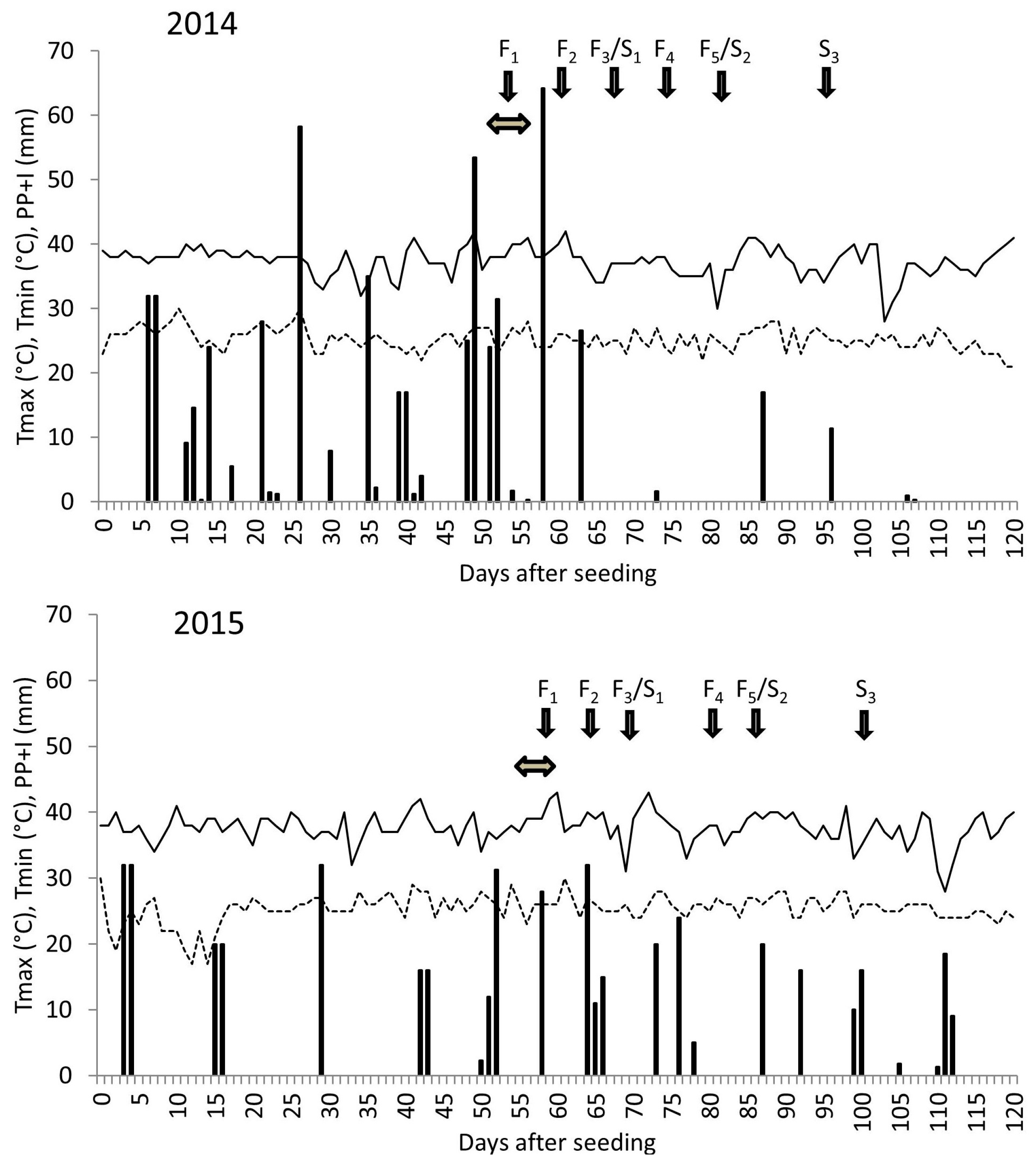
2.1. Field Experiments

The field experiments were conducted at the CIMMYT experimental station in Ciudad Obregon, Sonora, Mexico (27°20′N, 109°54′W, 38 m above sea level) during the 2014 and 2015 summer seasons. Different sets and numbers of hybrids were used in eighteen experiments (

Table 1. Description of vegetative indices under study. Equation used in the calculation, traits related, and reference.

Index	Equation	Traits Ralated	Reference
NDVI	(R800 − R670)/(R800 + R670)	Productivity	[25,26]
		Greenness
		Canopy cover
CWMI	R800/R710	Crop weight mass	[28]
HBSI	(R800 − R670)/(R800 + R670)	Biomass	[27]
GRE	500*((R800/R710) − 1) + 27	Chlorophyll content	[26]

). Hybrids were of tropical/subtropical adaptation, developed by CIMMYT for use in Latin America. Eleven experiments were carried out in 2014 (OB14-1 to 11) and seven in 2015 (OB15-1 to 7) following the same management protocols. The experiments were aimed at experiencing moderate drought stress at flowering and during the grain filling period. For that, irrigation was reduced to 50% of potential evapotranspiration, starting 12–15 days (~190 GDD) before flowering. Irrigation was applied on a weekly basis using drip irrigation at a rate of 5 mm/h for 6–14 h, depending on the potential evapotranspiration and the crop stage. Experiments were seeded on 20 June in 2014 and 1 June in 2015. Experiments were laid out in an alpha-lattice (0, 1) design, replicated twice with incomplete block sizes of five. Plots consisted of two maize rows, 4.5 m long, at a row spacing of 0.75 m. Plots were hand-seeded with two seeds per hill and thinned to one plant per hill (46 plants per plot; 6.6 plants per m⁻²) three weeks after planting. All plots received an initial application of 100 kg·ha⁻¹ of mono-ammonium phosphate (NH₄)H₂PO₄ and 500 kg·ha⁻¹ of ammonium sulfate ((NH₄)₂SO₄) at sowing. A second application of 250 kg·ha⁻¹ of ammonium sulfate was applied at V5. Weeds, insects, and diseases were controlled as needed.

2.2. Measurements and Calculations

The anthesis date was recorded when 50% of the plants within a plot had shed pollen. Plots were visited every 2–3 days to monitor anthesis evolution. Two, four, and six weeks after flowering (i.e., the approximate date when average flowering for all experiments within each year was reached) senescence was measured visually using a scale ranging from one (no senescence) to nine (complete senescence), as described earlier [21]. Senescence scores were converted to stay-green for each date of recording as: stay-green = 10 − senescence. After physiological maturity was reached, all the ears of each plot were collected and shelled and grain weight and moisture were recorded. The grain yield is reported at 12% moisture.

For senescence, the area under the curve (AUC) during the period from recording date one to three (_AUCSEN) was calculated by integrating a polynomial function of the second degree fitted to individual measurements. For stay-green, AUC (_AUCSG) was calculated by integrating stay-green from the flowering date of each individual plot for a constant period of time for all plots within each experiment. The period of integration was calculated as the number of days from the anthesis of the first flowering plot within the experiment until the date of last stay-green (stay-green = 10 − senescence) measurement (i.e., recording number three). For the period from flowering to the first date of stay-green recording, a stay-green value of nine was considered each day. To estimate daily stay-green from the first scoring date until the last day of integration, a polynomial model of the second degree of stay-green as a function of days was fitted. The model was fitted using scores from the three visual senescence readings; two, four, and six weeks after flowering.

In both years, plots were imaged with a multispectral imager (Tetracam, Chatsworth, CA, USA) on-board of a Piper PA-16 Clipper (Piper, Vero Beach, FL, USA) five times at weekly intervals starting at the anthesis. The flight path followed an east to west and west to east flight pattern at an above ground altitude of 270 m and at a ground speed of 33.33 m·s⁻¹. The multispectral camera had a radiometric resolution of 10 bits, configured at six bands with wavelengths of 550, 670, 700, 710, 750, and 800 nm. The imagery was atmospherically corrected with irradiance information produced on the basis of the data collected with the sun photometer on the flight day. The processing resulted in a pair of reflectance data images (range 0–100,000) for each frame captured, with three bands stored in each image, summing the six bands acquired. The first image of the pairs was mosaicked with the software Autopano (Version 3.0, Kolor, Francin, France) to create a single image for the whole area. The second image of the pairs was mosaicked with the exact same parameters used for the first image of the pair. Both 3-band images were merged into one 6-band image with ENVI software (Version 5.0, Exelis Visual Information Solutions, Boulder, CO, USA). The images were then manually geo-referenced using an image-to-image registration. The image used as reference was a 30 cm world imagery basemap. After image correction, image pixel information was extracted from the plots seen on it, using the QGIS software (QGIS Development Team, 2013, QGIS Geographic Information System; Open Source Geospatial Foundation Project). To transform the pixel values to tabular data, the mean value was obtained from the pixels whose center was inside each individual plot. The plots were represented as 4.5 m × 0.8 m polygons (in shape file format) with the individual unique attributes of the experiment and plot they represent. They were also geo-referenced. In cases where the plot polygons did not correctly match the image, the polygons were manually aligned to the plots with the ‘affine transformations’ plugin (QGIS, Newcastle, UK). Once the plots matched the images, a buffer was created to get an area that is smaller on each side than the experimental plots, keeping the central area of each plot to avoid borders. The mean values of reflectance were calculated using the ‘ZonalStats’ plugin (QGIS, Newcastle, UK), generating a table with columns, indicating plot-ID and the mean value obtained from the pixels of the image file. Using the reflectance data obtained with the multispectral camera, different vegetative indices were calculated for each plot on each flight date. A description of each index is presented in Table 1.

For each of the vegetative indices, AUC (i.e., _AUCNDVI, _AUCCWMI, _AUCHBSI and _AUCGRE) was calculated using the same methodology as for _AUCSG. For each plot, the AUC for each index was calculated by integrating the daily values from the anthesis date of each plot for a constant period of time for all plots within each experiment. The period of integration was calculated, as the number of days from the anthesis of the first flowering plot within the experiment until the date of the last flight. From flowering to the first flight, the daily vegetative indices values were considered to be the same as recorded at flight one. To estimate the daily vegetative indices values from the first scoring date until the last day of integration, a polynomial model of the second degree of the vegetative index as a function of days was fitted. The model was fitted using the scores recorded on flights one to five.

Another methodology to study canopy senescence through vegetative indices was proposed by calculating the reduction on the AUC for flights 4 and 5, relative to the AUC for flights 1 and 2. That relative reduction in AUC was calculated for NDVI, CWMI, HBSI and GRE (_ΔNDVI, _ΔCWMI, _ΔHBSI and _ΔGRE, respectively) as follows the example for NDVI:

_ΔNDVI = _AUCNDVI_fl4–5/_AUCNDVI_fl1–2

where _AUCNDVI_fl4–5 and _AUCNDVI_fl1–2 are the AUC for flights 4 and 5, and for flights 1 and 2, respectively.

2.3. Statistical Analysis

Data were analyzed with a linear mixed model containing the overall mean µ, block effect βi, genotype effect αj, and experimental error eij to explain the response variable Yij in the below model:

Yij = µ + βi + αj + eij

The genotype was treated as fixed and the error as random. The variance components were estimated by restricted maximum likelihood (REML) and heritability as the relationship between genetic and phenotypic variance, as per the formula:

$$h^2=\frac{{\mathsf{\sigma }}_{\mathrm{g}}^2}{\raisebox{1ex}{${\mathsf{\sigma }}_{\mathrm{g}}^2+{\mathsf{\sigma }}_{\mathrm{g}}^2$}\!\left/ \!\raisebox{-1ex}{$\mathrm{r}$}\right.}$$

The best linear unbiased predictors (BLUP) of genotypes and broad sense heritability were obtained. The BLUPs for genotype effects are shrinkage predictors, obtained as:

$$\tilde{\mathsf{\alpha }}=\hat{\mathrm{G}}{\mathrm{Z}}^{\prime }{\hat{\mathrm{V}}}^{-1}\left(\mathsf{\gamma }-1\mathsf{\mu }\right)$$

where y is the vector of the response variable, $\hat{\mathrm{G}}$ the matrix of variance covariance of the random effects, $\mathrm{Z}$ the design matrix for random effects in the model, $\hat{\mathrm{V}}$ is the estimated variance of y, 1 is a vector of ones, and µ is the overall mean, the only fixed parameter in the model. Genetic correlations among traits were computed as r_A = [Cov_A)/(δ_A(X).δ_A(Y))], in which r_A is the genetic correlation between X and Y, Cov_A is the genetic covariance between X and Y, δ_A(X) is the genetic standard deviation of X, and δ_A(Y) is the genetic standard deviation of Y [32]. The genetic correlations provide a measure of the strength of the agreement between the genotype rankings for two different traits. All calculations were performed within the R-environment (R Core Development Team 2009), using the program Multi Environment Trial Analysis with R for Windows (META-R, [33]).

3. Results

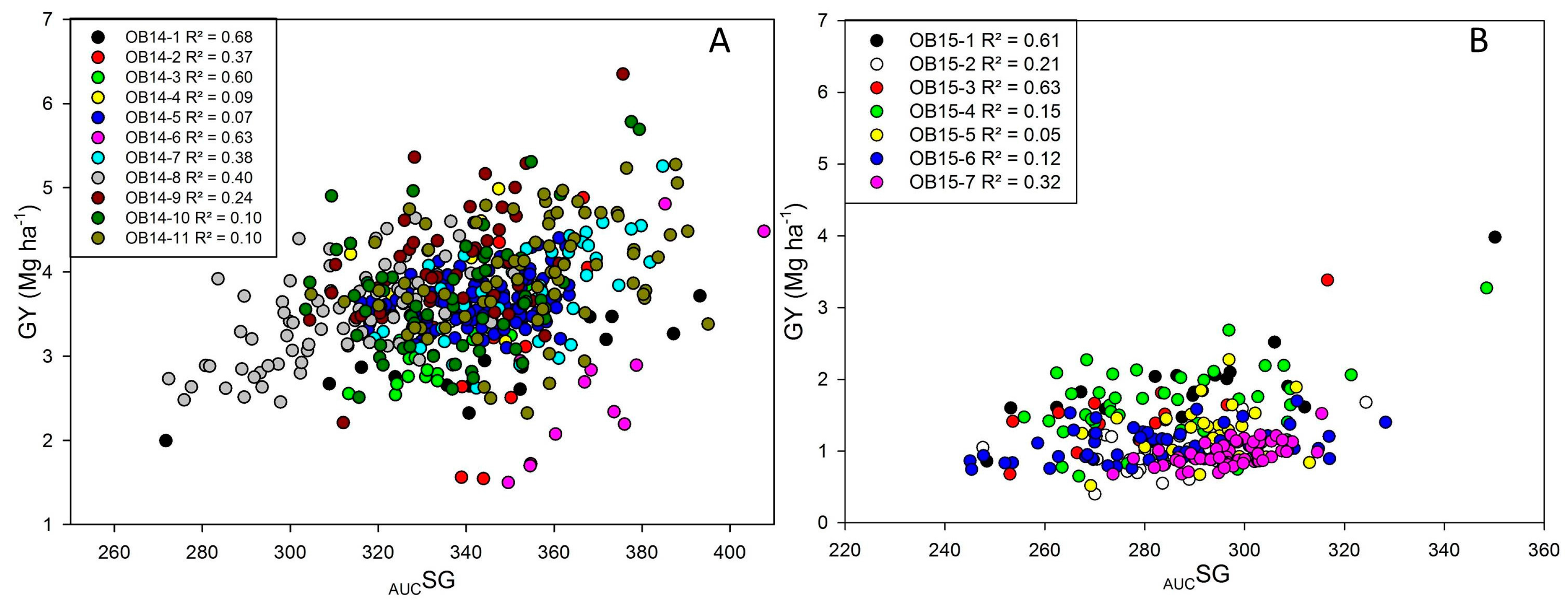
3.1. Grain Yield and Stay-Green

Experiments conducted in 2014 and 2015 were aimed to experience heat in combination with moderate drought stress around and after flowering. The temperature regime during the crop cycle was similar in both years, characterized by a high average temperature (31.3 and 31.5 °C in 2014 and 2015, respectively), a high average daily maximum temperature (37.3 and 37.6 °C in 2014 and 2015, respectively), and an elevated frequency of days with temperatures above 34 °C of 0.88 and 0.93 for 2014 and 2015, respectively (Figure 1). Heavy rains around and after flowering in 2014 resulted in moderate drought stress only. This was reflected in the average grain yields of 3.49 Mg·ha⁻¹ in 2014 and 1.33 Mg·ha⁻¹ in 2015 (

Table 2. Description of trials’ replication number, genotype number, trial mean for anthesis date (days from seeding), grain yield (GY, Mg·ha⁻¹), stay-green (_AUCSG), and heritability for GY and _AUCSG (SG) and the interquartile (IQ) range for GY and _AUCSG (SG).

Trial ID	Reps	Genotypes	Year	Trial Mean			Heritability		IQ Range
				Anthesis	GY	SG	GY	SG	GY	SG
OB14-1	3	16	2014	52	2.92	345	0.91	0.73	0.64	48.6
OB14-2	3	12	2014	58	3.04	348	0.90	0.76	1.55	35.8
OB14-3	3	21	2014	56	3.09	334	0.88	0.81	0.85	49.1
OB14-4	3	15	2014	54	3.89	335	0.88	0.89	0.85	26.7
OB14-5	2	116	2014	54	3.66	343	0.98	0.86	0.90	37.2
OB14-6	3	12	2014	57	2.68	369	0.64	0.47	1.13	26.4
OB14-7	2	39	2014	55	3.80	354	0.87	0.86	1.13	36.6
OB14-8	3	76	2014	55	3.49	311	0.48	0.63	1.10	36.3
OB14-9	2	45	2014	53	4.09	336	0.98	0.87	0.90	40.2
OB14-10	2	60	2014	52	3.71	336	0.79	0.81	0.80	37.0
OB14-11	2	75	2014	52	4.00	354	0.85	0.81	1.15	38.3
OB15-1	3	20	2015	59	1.85	288	0.92	0.93	0.90	25.5
OB15-2	3	20	2015	58	0.95	282	0.90	0.77	0.68	35.1
OB15-3	2	12	2015	59	1.55	277	0.97	0.74	0.50	23.7
OB15-4	2	44	2015	59	1.64	285	0.88	0.84	0.80	37.2
OB15-5	2	28	2015	59	1.27	291	0.80	0.71	0.65	29.5
OB15-6	2	60	2015	55	1.08	284	0.58	0.75	0.70	42.2
OB15-7	2	60	2015	55	0.96	297	0.37	0.48	1.00	40.6

). The heritability for grain yield was high in both years with values up to 0.98, with the exception of experiments OB14-8 and OB14-7 with values of 0.48 and 0.37, respectively. The inter-quartile range of grain yield for the individual plots averaged at 1 and 0.75 Mg·ha⁻¹ for 2014 and 2015, respectively. The inter-quartile range relative to the mean grain yield was higher for 2015 than for 2014 (0.8 and 0.3, respectively).

The _AUCSG was larger for 2014 than for 2015, also as an expected result of different stress levels, ranging from 311 to 369 in 2014 and from 277 to 297 in 2015 (Table 2). The heritability of _AUCSG was also high for most experiments in both years (averaged 0.77 and 0.75 in 2014 and 2015, respectively), but moderate for OB14-6 and OB15-7, with values of 0.47 and 0.48, respectively. The inter-quartile range for _AUCSG was 37 for both years. When calculated relative to the mean, the inter-quartile range for _AUCSG was smaller than for grain yield and slightly larger in 2015 than in 2014 (0.109 and 0.125 for 2014 and 2015, respectively).

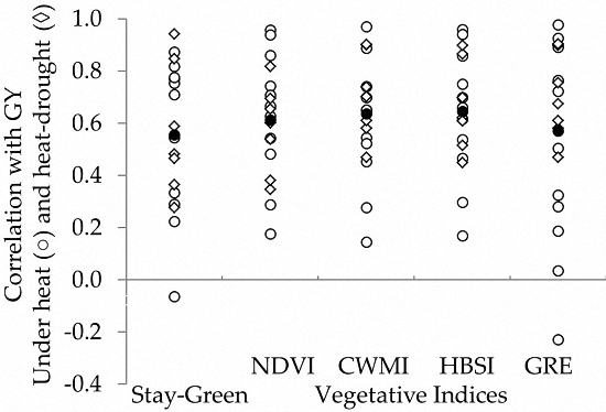
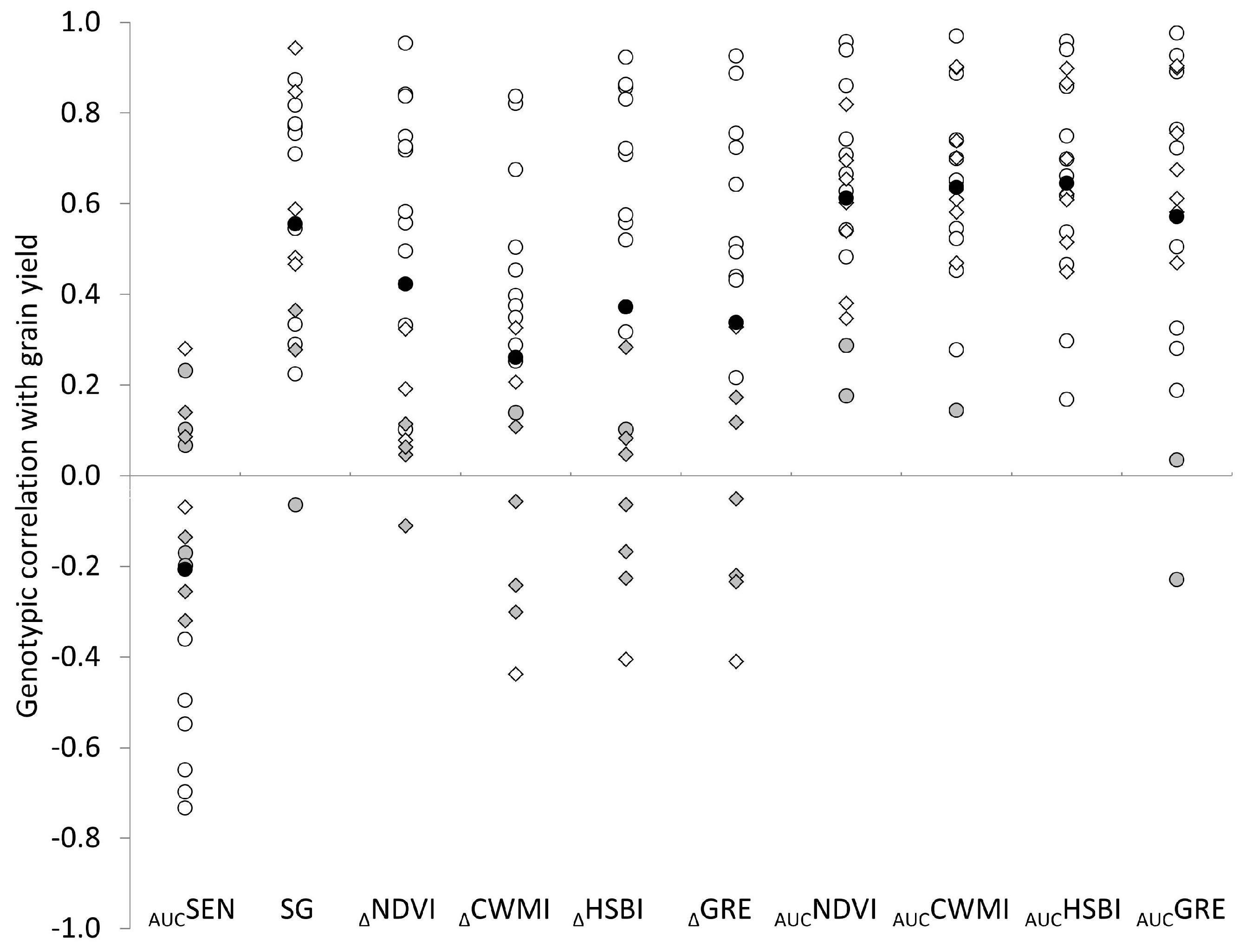
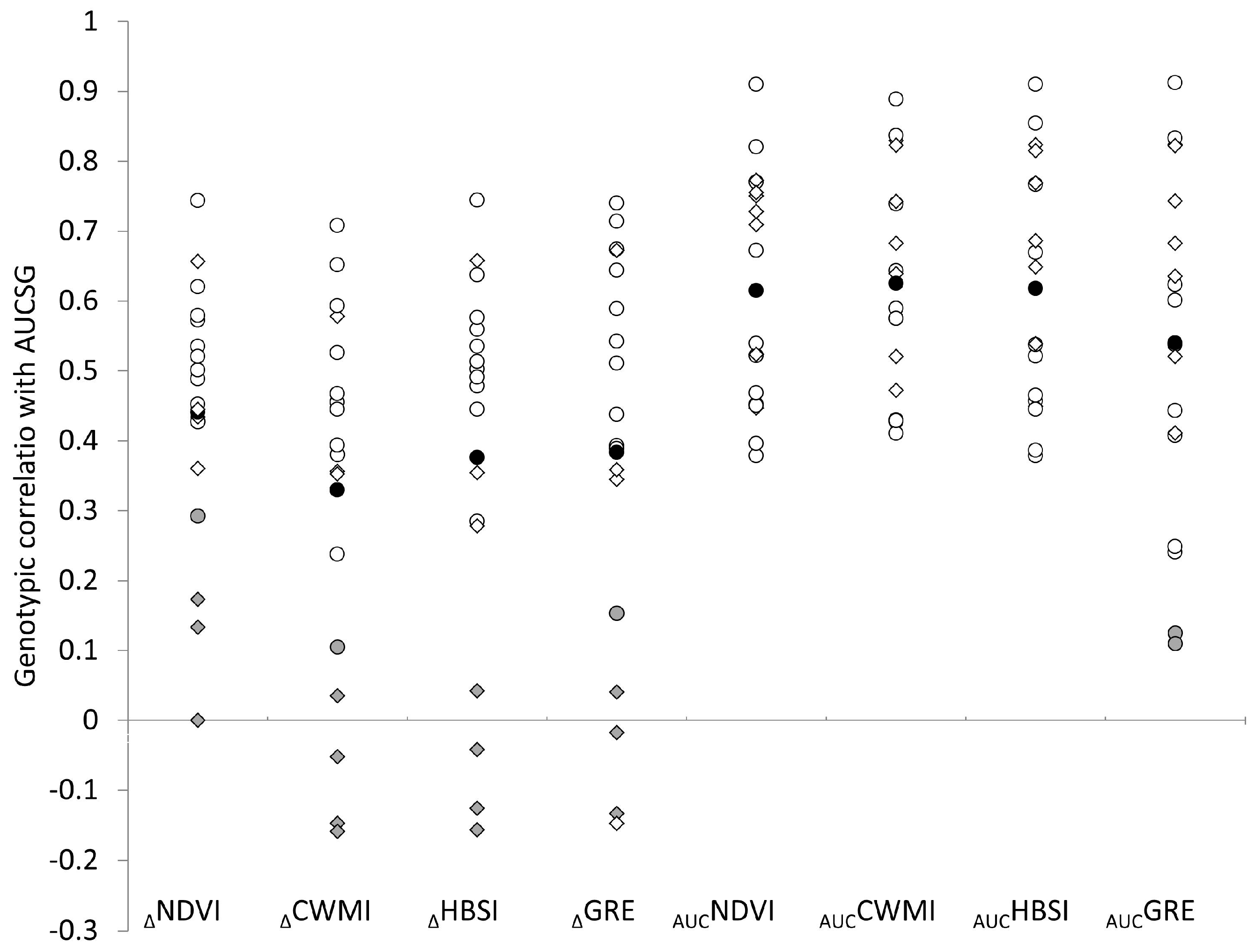
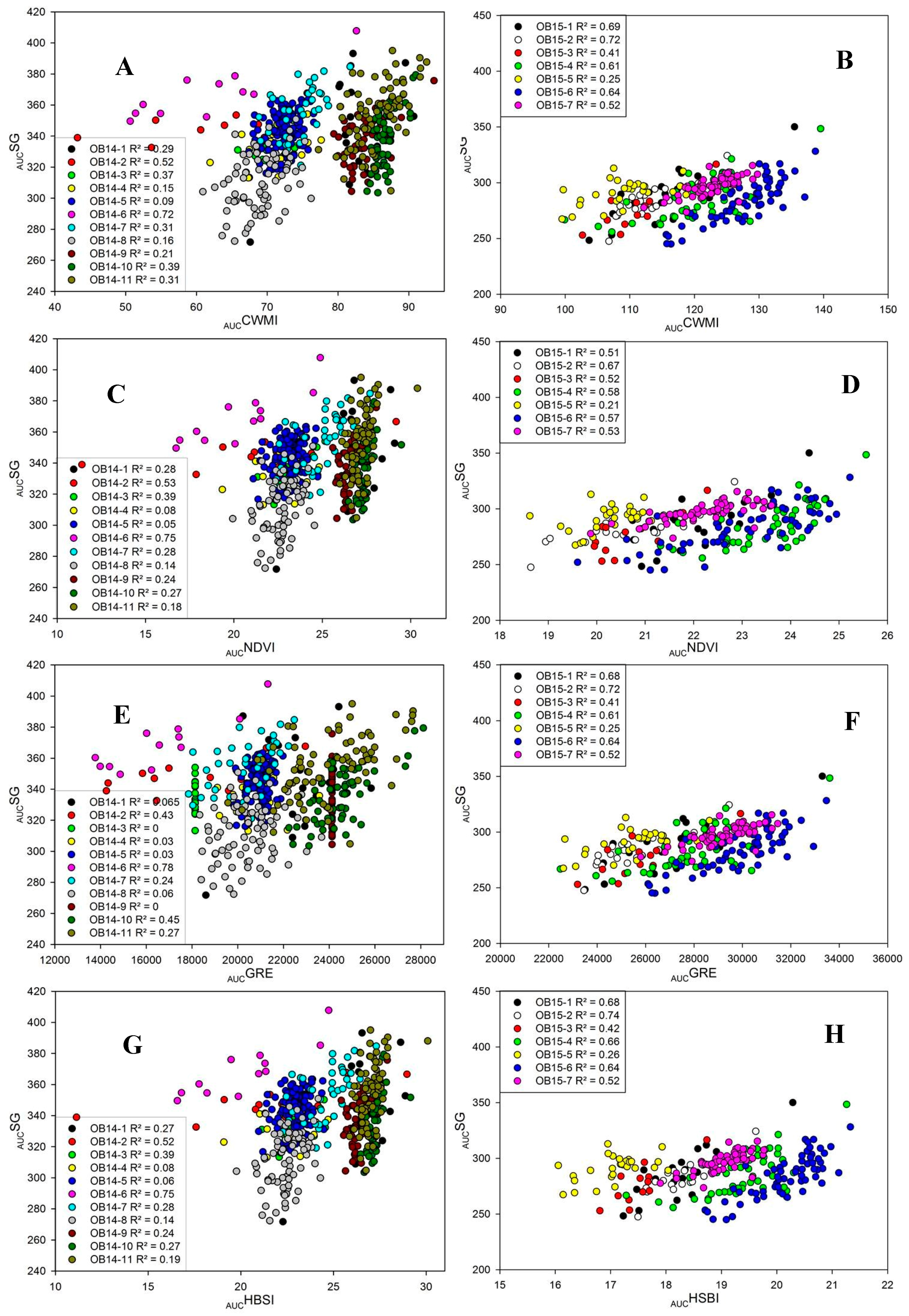
3.2. Genotypic Correlations of Traits with Grain Yield

Genotypic correlations with grain yield differed among traits and among methods of calculations for the vegetative indices (Figure 2). The _AUCSEN, a trait that is not adjusted for different flowering dates, had low average and variable correlation values with grain yield, both in 2014 and 2015 (average of −0.31 and −0.03, respectively). Similarly vegetative indices not adjusted for different flowering dates (i.e., _ΔNDVI, _ΔCWMI, _ΔHBSI and _ΔGRE) had lower correlation values with grain yield than the AUC for the same traits and were markedly lower for 2015 relative to 2014. The within year averages for correlations with grain yield were 0.61/0.10, 0.46/−0.05, 0.60/0.06, and 0.57/−0.04 for _ΔNDVI, _ΔCWMI, _ΔHBSI, and _ΔGRE in 2014/2015, respectively.

Traits that take into account the period from flowering to time of scoring on the integral calculation (i.e., _AUCSG, _AUCNDVI, _AUCCWMI, _AUCHBSI, and _AUCGRE) correlated better with grain yield and had reduced variability among years (Figure 2 and Figure 3), relative to the differential method. The _AUCSG had moderate values of genotypic correlation with grain yield across years, with average values of 0.55 (ranging from −0.06 to 0.87) and 0.56 (ranging from 0.28 to 0.94) for 2014 and 2015, respectively. Similarly, vegetative indices had correlation coefficients that ranged from 0.49 (_AUCGRE in 2014) to 0.70 (_AUCCWMI in 2015) for all the experiments within a year on average. The correlation of the AUC for vegetative indices with grain yield were larger in 2015 than in 2014; as an average for _AUCNDVI, _AUCCWMI, _AUCHBSI, and _AUCGRE traits, correlation values were 0.59 and 0.66 for 2014 and 2015, respectively. Stronger correlations for 2015 could be related to the greater stress intensity resulting in greater segregation among hybrids in 2015.

When averaged across all experiments, genotypic correlations with _AUCSG were moderate for _AUCCWMI (r_g = 0.76), _AUCNDVI (r_g = 0.72), and _AUCHBSI (r_g = 0.71) while slightly lower and more variable for _AUCGRE (r_g = 0.61) (Figure 4 and Figure 5). For all four traits, genotypic correlations were stronger in 2015 than 2014, with averages for the four traits of 0.77 and 0.66, respectively. The difference between years may be explained by greater stress intensity, resulting in greater genotypic segregation and in a larger interquartile range for _AUCSG in 2015.

The traits not corrected for flowering dates (i.e., _ΔNDVI, _ΔCWMI, _ΔHBSI and _ΔGRE) had lower values of genotypic correlation with _AUCSG than AUC traits corrected for flowering dates (Figure 4 and Figure 5). Moreover, the differences for correlation coefficients between 2014 and 2015 were large for _ΔCWMI, _ΔHBSI, and _ΔGRE, while less pronounced for _ΔNDVI. For the within year average, correlation coefficients averaged 0.64/0.30, 0.53/0.15, 0.66/0.15, and 0.66/0.17 for 2014/15 of _ΔNDVI, _ΔCWMI, _ΔHBSI, and _ΔGRE, respectively.

4. Discussion

Although all the experiments aimed to experience combined drought and heat stress at flowering and during the grain filling period, heavy rains around flowering in 2014 resulted in drought stress during the grain filling period only. Heat stress, however, was consistent throughout the season in both years, as reflected by both the mean daily maximum temperature (37.3 and 37.6 °C for 2014 and 2015, respectively) and the frequency of days with temperatures above the optimum (0.88 and 0.93 for 2014 and 2015, respectively). Compared to experiments carried out by CIMMYT using germplasm of similar genetic background under non-stressed conditions [14,34,35], grain yield was 53% and 82% lower for the experiments carried out in 2014 and 2015, respectively. These large yield reductions as a result of heat and combined heat and drought stress reflect the synergy of both stress factors when they occur together, as reported earlier [8]. Moreover, these results re-emphasize the need for a better understanding of physiological interrelations and the genetic basis of tolerance under heat stress. The heritability of grain yield was high for both years (h² = 0.37–0.98), under both stress conditions (heat and combined heat and drought stress).

Stay-green (or delayed leaf senescence; [15]) is related to physiological maturity and allows selecting for germplasm with an extended grain filling period [14] and a resulting high grain yield. We calculated the _AUCSG trait based on visual senescence scores. In contrast to traditionally used _AUCSEN, _AUCSG integrates the value of stay-green during a period of constant duration (within each experiment) in the comparison among hybrids. As such, it is not biased by the flowering date and is better related to the grain filling period than _AUCSEN. A better relation of _AUCSG to actual grain filling duration may explain its higher correlation with grain yield relative to _AUCSEN. Averaged across experiments, _AUCSG was lower in 2015 relative to 2014 as a result of larger stress experienced during 2015, whereas the correlation of _AUCSG with grain yield was similar in both years (r_g = 0.56 and 0.50 for 2014 and 2015, respectively). Stability across years, correlations with grain yield, and high heritability (h² = 0.48–0.93), in addition to importance of stay-green shown in the past [34,35], make _AUCSG a useful secondary trait for use in breeding programs in which target environments are characterized by frequent droughts after flowering and are exposed to heat stress. Although all trials in this study were exposed to stress around flowering and grain filling, it is expected that _AUCSG is also a useful secondary trait under non-stressed conditions [14,19].

Two methodologies using either the AUC or the relative difference between the first two and last two measurements were used to predict grain yield and _AUCSG using vegetative indices. The AUC for vegetative indices (on average for all traits in both years; r_g = 0.62) generally showed stronger and more stable associations with grain yield than the differential method (r_g = 0.35). Moreover, the AUC for vegetative traits was a good estimator of _AUCSG (on average for all traits in both years; r_g = 0.70). While the differential methodology is relatively easier to calculate, it would not be as good an estimator for grain yield as the AUC (r_g = 0.46). While differential traits showed lower correlation with grain yield than traits calculated as AUC, _ΔNDVI had larger and more consistent correlation values than _AUCSEN. Due to its simple protocol for measurement and computation, _ΔNDVI might nevertheless be a useful secondary trait for remote trial locations where flowering time is not recorded and visual recordings are not taken.

The use of airborne platform mounted cameras to collect information in a fast and cost-effective way offers the throughput as needed in a breeding environment [31]. Using a multispectral camera mounted to an airplane allowed us to identify several spectral indices with good correlation to grain yield; _AUCNDVI (r_g = 0.62), _AUCHBSI (r_g = 0.64), _AUCGRE (r_g = 0.57), and _AUCCWMI (r_g = 0.63) were associated with grain yield across experiments and years. The strongest and most stable association with grain yield was found for NDVI. NDVI is a vegetative index widely studied in different crops, which relates to greenness and radiation interception [25]. Because of its high heritability (h² = 0.41–0.96, average 0.70), relatively high and stable association (r_g = 0.18–0.96, average 0.62) with grain yield, and senescence, it is rendered a suitable trait for use in breeding programs. Since the flight campaign in both years ended before complete senescence was reached, it is not clear to what extent later measurements could have improved association with grain yield or _AUCSG.

The AUCs of vegetative indices are not only good estimators of grain yield, but they are also moderately to highly associated with _AUCSG (r_g = 0.70 averaged across trials and years). Those indices showed stronger and more stable associations with _AUCSG than indices calculated with the differential method (r_g = 0.46), which may be explained by the similar calculation methodology of _AUCSG and the AUC of vegetative indices. Among the AUC indices, the strongest and more stable association with _AUCSG was found for _AUCCWMI (r_g = 0.76), _AUCNDVI (r_g = 0.72) and _AUCHBSI (r_g = 0.71), compared to _AUCGRE (r_g = 0.61). The strong association of the vegetative indices used here with stay-green suggests that they may also have a good correlation with the length of the grain filling period [14]. This could be useful in situations in which the combination of an early flowering with a long grain filling period would ensure drought escape in dry years but ensure high grain yields in the absence of stress, as demonstrated earlier [14,36]. When the vegetative index traits were calculated using a relative differential methodology (Δ), they had lower and less consistent correlations with _AUCSG than when they were calculated as AUC. Differences in the degree and consistency of these correlations can potentially be explained by the fact that the AUC values were corrected for the flowering date.

The _AUCNDVI is proposed as the best secondary trait to breed for high grain yield and extended stay-green under heat and combined heat and drought stresses. This is a trait with high heritability and moderate and consistent correlation with grain yield. Although the experiments were exposed to moderate to severe stress in this study, it is expected that _AUCNDVI also relates to grain yield under optimal conditions, as shown earlier [14,19]. Compared to earlier studies, using airborne platforms to measure _AUCNDVI would tremendously increase the throughput, allowing more measurements in more experiments. Good associations of _AUCNDVI with grain yield and stay-green in combination with high heritability will allow the use of _AUCNDVI in addition to grain yield in selection, facilitating the identification of climate resilient germplasm.

5. Conclusions

We present novel methodologies to measure and compute secondary traits to develop germplasm with high grain yield under heat and combined heat and drought stresses. Stay-green corrected for flowering dates showed higher and more stable correlation with grain yield relative to traditionally used _AUCSEN. _AUCNDVI (rGY = 0.62; r_AUCSG = 0.72), _AUCHBSI (rGY = 0.64; r_AUCSG = 0.71), _AUCGRE (rGY = 0.57; r_AUCSG = 0.61), and _AUCCWMI (rGY = 0.63; r_AUCSG = 0.75) were associated with grain yield and stay-green across experiments and years. The index _AUCNDVI is proposed as an effective and efficient secondary trait to select improved stay-green in tropical and subtropical germplasm, in addition to grain yield, to identify climate resilient germplasm to increase food security in a changing climate.

References

1. Chowdhury, S.I.; Wardlaw, I.F. The effect of temperature on kernel development in cereals. Aust. J. Agric. Res. 1978, 29, 205–223. [Google Scholar] [CrossRef]
2. Ellis, R.H.; Summerfield, R.J.; Edmeades, G.O.; Roberts, E.H. Photoperiod, temperature, and the interval from sowing to tassel initiation in diverse cultivars of maize. Crop Sci. 1992, 32, 12–25. [Google Scholar] [CrossRef]
3. Shaw, R.H. Estimates of yield reductions in corn caused by water and temperature stress. In Crop Reactions to Water and Temperature Stresses in Humid and Temperate Climates; Raper, C.D., Kramer, P.J., Eds.; Westview Press: Boulder, CO, USA, 1983; pp. 49–65. [Google Scholar]
4. Rattalino Edreira, J.I.; Otegui, M.E. Heat stress in temperate and tropical maize hybrids: Differences in crop growth, biomass partitioning and reserves use. Field Crop. Res. 2012, 130, 87–98. [Google Scholar] [CrossRef]
5. Neiff, N.; Trachsel, S.; Valentinuz, O.R.; Balbi, C.N.; Andrade, F.H. High temperatures around flowering in maize: Effects on photosynthesis and grain yield in three genotypes. Crop Sci. 2016, 56, 2702–2712. [Google Scholar]
6. Rosenzweig, C.; Elliott, J.; Deryng, D.; Ruane, A.C.; Müller, C.; Arneth, A.; Boote, K.J.; Folberth, C.; Glotter, M.; Khabarov, N.; et al. Assessing agricultural risks of climate change in the 21st century in a global gridded crop model intercomparison. Proc. Natl. Acad. Sci. USA 2014, 111, 3268–3273. [Google Scholar] [CrossRef] [PubMed]
7. Porter, J.R.; Xie, L.; Challinor, A.J.; Cochrane, K.; Howden, S.M.; Iqbal, M.M.; Travasso, M.I. Food security and food production systems. In Climate Change 2014–Impacts, Adaptation and Vulnerability. Part A Global and Sectoral Aspects; Contribution Working Group II to Fifth Assessment Report; Intergovernmental Panel on Climate Change: Geneva, Switzerland, 2014; pp. 485–533. [Google Scholar]
8. Lobell, D.B.; Bänziger, M.; Magorokosho, C.; Vivek, B. Nonlinear heat effects on African maize as evidenced by historical yield trials. Nat. Clim. Chang. 2011, 1, 42–45. [Google Scholar] [CrossRef]
9. Mugo, S.N.; Njoroge, K. Alleviating the effects of drought on maize production in the moisture stress areas of Kenya through escape and tolerance. In Proceedings of the Developing Drought- and Low N-Tolerant Maize, Proceedings of a Symposium, El Batan, Mexico, 25–29 March 1997.
10. Monneveux, P.; Sanchez, C.; Tiessen, A. Future progress in drought tolerance in maize needs new secondary traits and cross combinations. J. Agric. Sci. 2008, 146, 287–300. [Google Scholar] [CrossRef]
11. Blum, A. Plant Breeding for Stress Environments; CRC Press: Boca Raton, FL, USA, 1988; p. 223. [Google Scholar]
12. Mugo, S.N.; Smith, M.E.; Banziger, M.; Setter, T.L.; Edmeades, G.O.; Elings, A. Performance of early maturing Katumani and Kito maize composites under drought at the seedling and flowering stages. Afr. Crop Sci. J. 1998, 6, 329–344. [Google Scholar] [CrossRef]
13. Bruns, H.A.; Abbas, H.K. Planting date effects on Bt and Non-Bt corn in the Mid-South USA. Agron. J. 2006, 98, 100–106. [Google Scholar] [CrossRef]
14. Trachsel, S.; Burgueno, J.; Suarez, E.A.; San Vicente, F.M.; Rodriguez, C.S.; Dhliwayo, T. Interrelations among early vigor, flowering time, physiological maturity, and grain yield in tropical maize (Zea mays L.) under multiple abiotic stresses. Crop Sci. 2017, 57, 1–14. [Google Scholar] [CrossRef]
15. Thomas, H.; Howarth, C.J. Five ways to stay-green. J. Exp. Bot. 2000, 51, 329–337. [Google Scholar] [CrossRef] [PubMed]
16. Tollenaar, M.; Wu, J. Yield improvement in temperate maize is attributable to greater stress tolerance. Crop Sci. 1999, 39, 1597–1604. [Google Scholar] [CrossRef]
17. Chapman, S.C.; Edmeades, G.O. Genotype by environment effects and selection for drought tolerance in tropical maize I. Two mode pattern analysis of yield. Euphytica 1997, 95, 1–9. [Google Scholar] [CrossRef]
18. Bänziger, M.; Lafitte, H.R. Efficiency of secondary traits for improving maize for low-nitrogen target environments. Crop Sci. 1997, 37, 1110–1117. [Google Scholar] [CrossRef]
19. Cairns, J.E.; Sanchez, C.; Vargas, M.; Ordoñez, R.; Araus, J.L. Dissecting maize productivity: Ideotypes associated with grain yield under drought stress and well-watered conditions. J. Integr. Plant Biol. 2012, 54, 1007–1020. [Google Scholar] [CrossRef] [PubMed]
20. Pinto, R.S.; Lopes, M.S.; Collins, N.C.; Reynolds, M.P. Modelling and genetic dissection of staygreen under heat stress. Theor. Appl. Genet. 2016, 129, 2055–2074. [Google Scholar] [CrossRef] [PubMed]
21. Bänziger, M.; Edmeades, G.O.; Beck, D.; Bellon, M. Breeding for Drought and Nitrogen Stress Tolerance in Maize: From Theory to Practice; Cimmyt: Mexico Distrito Federal, Mexico, 2000. [Google Scholar]
22. Vina, A.; Gitelson, A.A.; Rundquist, D.C.; Keydan, G.; Leavitt, B.; Schepers, J. Remote sensing—Monitoring maize (Zea mays L.) phenology with remote sensing. Agron. J. 2004, 96, 1139–1147. [Google Scholar] [CrossRef]
23. Liebisch, F.; Kirchgessner, N.; Schneider, D.; Walter, A.; Hund, A. Remote, aerial phenotyping of maize traits with a mobile multi-sensor approach. Plant Methods 2015, 11, 1746–4811. [Google Scholar] [CrossRef] [PubMed]
24. Li, L.; Zhang, Q.; Huang, D.A. Review of imaging techniques for plant phenotyping. Sensors 2014, 14, 20078–20111. [Google Scholar] [CrossRef] [PubMed]
25. Tucker, C.J. Red and photographic infrared linear combinations for monitoring vegetation. Remote Sens. Environ. 1979, 8, 127–150. [Google Scholar] [CrossRef]
26. Gitelson, A.A.; Viña, A.; Arkebauer, T.J.; Rundquist, D.C.; Keydan, G.; Leavitt, B. Remote estimation of leaf area index and green leaf biomass in maize canopies. Geophys. Res. Lett. 2003, 30. [Google Scholar] [CrossRef]
27. Thenkabail, P.S.; Murali Krishna Gumma, P.T.; Mohammed, I. Hyperspectral remote sensing of vegetation and agricultural crops. Photogramm. Eng. Remote Sens. 2014, 80, 679–710. [Google Scholar]
28. Winterhalter, L.; Mistele, B.; Jampatong, S.; Schmidhalter, U. High-throughput sensing of aerial biomass and above-ground nitrogen uptake in the vegetative stage of well-watered and drought stressed tropical maize hybrids. Crop Sci. 2011, 51, 479–489. [Google Scholar] [CrossRef]
29. Weber, V.S.; Araus, J.L.; Cairns, J.E.; Sanchez, C.; Melchinger, A.E.; Orsini, E. Prediction of grain yield using reflectance spectra of canopy and leaves in maize plants grown under different water regimes. Field Crop. Res. 2012, 128, 82–90. [Google Scholar] [CrossRef]
30. Romano, G.; Zia, S.; Spreer, W.; Sanchez, C.; Cairns, J.; Araus, J.L.; Müller, J. Use of thermography for high throughput phenotyping of tropical maize adaptation in water stress. Comput. Electron. Agric. 2011, 79, 67–74. [Google Scholar] [CrossRef]
31. Neiff, N.; Dhliwayo, T.; Suarez, E.A.; Burgueno, J.; Trachsel, S. Using an airborne platform to measure canopy temperature and NDVI under heat stress in maize using an airborne platform to measure canopy temperature and NDVI under heat stress. J. Crop Improv. 2015, 29, 669–690. [Google Scholar] [CrossRef]
32. Cooper, M.; Delacy, I.H. Relationships among analytical methods used to study genotypic variation and genotype-by-environment interaction in plant breeding multi-environment experiments. Theor. Appl. Genet. 1994, 88, 561–572. [Google Scholar] [CrossRef] [PubMed]
33. Alvarado, G.M.; López, M.; Vargas, A.; Pacheco, F.; Rodríguez, J.; Burgueño, J.; Crossa, J. META-R (Multi Environment Trial Analysis with R for Windows) Version 5.0; International Maize and Wheat Improvement Center: Texcoco, Mexico, 2015. [Google Scholar]
34. Almeida, G.D.; Makumbi, D.; Magorokosho, C.; Nair, S.; Borm, A.; Ribaut, J.M.; Banziger, M.; Prasanna, B.M.; Crossa, J.; Babu, R. QTL mapping in three tropical maize populations reveals a set of constitutive and adaptive genomic regions for drought tolerance. Theor. Appl. Genet. 2013, 126, 583–600. [Google Scholar] [CrossRef] [PubMed]
35. Trachsel, S.; Sun, D.; San Vicente, F.M.; Zheng, H.; Atlin, G.N.; Suarez, E.A.; Babu, R.; Zhang, X. Identification of QTL for early vigor and stay-green conferring tolerance to drought in two connected advanced backcross populations in tropical maize (Zea mays L.). PLoS ONE 2016, 11, e0149636. [Google Scholar]
36. Gasura, E.; Setimela, P.; Edema, R.; Gibson, P.T.; Okori, P.; Tarekegne, A. Exploiting grain-filling rate and effective grain-filling duration to improve grain yield of early-maturing maize. Crop Sci. 2013, 53, 2295–2303. [Google Scholar] [CrossRef]
Figure 1. Daily maximum temperature (full line), daily minimum temperature (dotted line), precipitations, and irrigations (bars) displayed in days after planting for experiments conducted in Obregon in 2014 and 2015. The horizontal arrow indicates the range of the average anthesis date for all trials. The vertical arrows indicate the dates of flights 1 to 5 (F1 to F5) and the dates of visual senescence scoring (S1, S2 and S3).
Remotesensing 09 00235 g001
Figure 2. Genotypic correlations of different traits with grain yield on 18 trials conducted in 2014 (○), 2015 (◊), and for the all trials’ mean (●). White and grey dots are different and not different from 0 at p < 0.05, respectively. The traits included stay-green (AUCSG), differential (Δ), and area under the curve (AUC) calculations for Normalized Difference Vegetative Index (NDVI), the crop water mass index (CWMI), HSBI1, the greenness (GRE), and the area under the curve (AUC) for senescence (AUCSEN).
Remotesensing 09 00235 g002
Figure 3. Association between best linear unbiased predictors (BLUP) for stay-green (AUCSG) and grain yield (GY) in eleven trials conducted in Obregon in 2014 (OB14-1 to 11; (A)) and in seven trials in 2015 (OB15-1 to 7; (B)). Results from different trials are represented by different symbols.
Remotesensing 09 00235 g003
Figure 4. Genotypic correlations of different traits with stay-green for 18 experiments conducted in 2014 (○), 2015 (◊), and for the all trial means (●).White and grey dots are different and not different from 0 at p < 0.05, respectively. The traits included were calculated using the differential method (Δ) and area under the curve (AUC) for NDVI, CWMI, HSBI1, and GRE.
Remotesensing 09 00235 g004
Figure 5. Associations among the best linear unbiased predictors (BLUP) for different vegetation indices and stay-green (AUCSG) in eleven trials conducted in Obregon in 2014 (OB14-1 to 11; (A,C,E,G)) and in seven trials in 2015 (OB15-1 to 7; (B,D,F,H)). The results from different trials are represented by different symbols.
Remotesensing 09 00235 g005