Mapping Above-Ground Biomass of Winter Oilseed Rape Using High Spatial Resolution Satellite Data at Parcel Scale under Waterlogging Conditions

Abstract

Oilseed rape (Brassica napus L.) is one of the three most important oil crops in China, and is regarded as a drought-tolerant oilseed crop. However, it is commonly sensitive to waterlogging, which usually refers to an adverse environment that limits crop development. Moreover, crop growth and soil irrigation can be monitored at a regional level using remote sensing data. High spatial resolution optical satellite sensors are very useful to capture and resist unfavorable field conditions at the sub-field scale. In this study, four different optical sensors, i.e., Pleiades-1A, Worldview-2, Worldview-3, and SPOT-6, were used to estimate the dry above-ground biomass (AGB) of oilseed rape and track the seasonal growth dynamics. In addition, three different soil water content field experiments were carried out at different oilseed rape growth stages from November 2014 to May 2015 in Northern Zhejiang province, China. As a significant indicator of crop productivity, AGB was measured during the seasonal growth stages of the oilseed rape at the experimental plots. Several representative vegetation indices (VIs) obtained from multiple satellite sensors were compared with the simultaneously-collected oilseed rape AGB. Results showed that the estimation model using the normalized difference vegetation index (NDVI) with a power regression model performed best through the seasonal growth dynamics, with the highest coefficient of determination (R² = 0.77), the smallest root mean square error (RMSE = 104.64 g/m²), and the relative RMSE (rRMSE = 21%). It is concluded that the use of selected VIs and high spatial multiple satellite data can significantly estimate AGB during the winter oilseed rape growth stages, and can be applied to map the variability of winter oilseed rape at the sub-field level under different waterlogging conditions, which is very promising in the application of agricultural irrigation and precision agriculture.

1. Introduction

Oilseed rape (Brassica napus L.) is one of the most important oil crops in China, and mainly grows from autumn to the beginning of the second year summer in the Yangtze River Basin, following by a paddy rice crop [1]. After the harvest of rice, oilseed rape was sowed in the excessive water stress paddy field, where it often suffers water-flooding in spring and summer and raining in autumns [2]. Therefore, oilseed rape is susceptible to waterlogging stress during growth stages. Waterlogging stress is a common natural disaster in the Yangtze River Basin, the annual occurrence of the affected area is generally 144.4 million hectares, accounting for more than 20% of the plant area [3]. The waterlogging stress caused by excessive or saturated soil moisture, can not only change the energy metabolism and physiological processes of the crops, but also impacts the cell structure, morphological features, and yield formation [4]. Although water is critical for crop growth, excessive water is harmful resulting in lower oxygen levels in the soil and may lead to serious consequences of necrosis, stunting, and defoliation [5]. Additionally, waterlogging also inhibits plant growth, reduces the accumulated amount of dry matter, and decreases yield drastically [6]. However, the impacts of waterlogging on different oilseed rape growth stages are different: at the seeding stage, waterlogging stress may lead to soil compaction, which may result in seed suffocation; at the seedling stage, waterlogging causes rape root damage and leaves became red, generally; at the flowering stage and podding stage, the waterlogging not only reduces buds, flowers and pods, decreasing the seed setting rate, but also causes sclerotinia [7]. Therefore, monitoring crop growth under waterlogging conditions is of great importance at different developmental periods in a target environment [8].

In recent years, many quantitative procedures have been proposed for water states based on the water budget and plant indicators, mainly based on sensing the plants’ response to water stress rather than directly detecting the soil moisture status [9]. Few studies have been conducted on different growth stages of field-grown oilseed rape under varying soil moisture [4,10,11]. Detailed field experiments have been predominantly directed toward analyzing the impacts of soil water content variability on physiological parameters and fruit yield [8,12,13]. Indeed, water productivity relates crop production to water use and is a key indicator for evaluating agricultural water management [9]. Information about vegetation growth and health in the developing season is crucial for optimizing crop production; leaf area index (LAI) and above-ground biomass (AGB) are some very useful indicators for crop growth and health, which can be used to guide the field managements as well as adjustments and requirements [14]. Traditional field validation of relevant parameters of cover crop growth through destructive sampling are time and cost intensive, which can become particularly cumbersome for regional studies [15]. Remote sensing offers a rapid and cost-effective way to capture valuable information about agriculture condition over large areas, which can greatly reduce the workload involved in crop investigation or in-field observation and offer the possibility to analyze plant biochemical conditions at a wide range of spatial scales [16]. Moreover, remote sensing techniques, as well as multispectral reflectance, can provide quantitative information about the water status of many agricultural crops [17,18]. Since the first satellite was launched in 1972, a fair amount of available remote sensing datasets and images have become the basic tools for land cover mapping, environmental monitoring, and ecological process scaling from stand to regional and global levels [19,20]. Meanwhile, time series observation is particularly important for monitoring seasonal changes in plant growth and development and for studying canopy function [21].

Most of previous studies adopted coarse- and moderate-resolution remote sensing data. For instance, the Advanced Very High Resolution Radiometer (AVHRR) (1.1 km spatial resolution at nadir), Moderate-resolution Imaging Spectroradiometer (MODIS) (two bands are imaged at a nominal resolution of 250 m at nadir, five bands at 500 m, and the remaining 29 bands at 1 km), and Landsat TM/ETM+ (30 m spatial resolution) have been used to estimate the canopy condition [22,23,24]. However, in many developing countries, smallholder farming is the main livelihood support for the majority of the population. When the field variability can be measured and monitored, site-specific knowledge can assist farmers and stakeholders in better management of their limited resources through new technologies in sustainable agricultural systems [25]. At the same time, the monitoring of crop growth conditions in smallholder agriculture requires higher spatial resolution satellite data.

Compared with coarse- and moderate-resolution satellite sensors, high spatial resolution optical satellite sensors have a relatively shorter revisiting cycle and are especially useful in capturing finer plant growth information [26]. In remote sensing, the applications of high spatial resolution optical satellite sensors can be used to obtain images with a spatial resolution of several meters and with a revisit cycle of less than five days, such as Pleiades-1 (0.5 m panchromatic resolution, 2 m multispectral resolution), Worldview-2 (0.46 m panchromatic resolution, 1.85 m multispectral resolution), Worldview-3 (0.31 m panchromatic resolution, 1.24 m multispectral resolution), IKONOS (0.82 m panchromatic resolution, 3.2 m multispectral resolution), and SPOT-6 (1.5 m panchromatic resolution, 6 m multispectral resolution) [27,28,29,30,31]. Multiple optical remote sensing sensors are suitable for acquiring time-series data and offer more chances to obtain cloud-free remote sensing images in a very short time, although they cannot escape the impact of constant thick cloud cover [32]. However, satellite data acquired from different sensors may not be comparable due to its own characteristics, i.e., orbital altitude, spatial and spectral resolutions, wavelength band limits, relative spectral responses of the sensors, etc. [33]. To model the multi-sensor bands, the spectral response function of each band must be convoluted between different sensors, and the empirical linear method was tested with a satisfactory result to calibrate the multi-sensor images [32]. Thus, for continuous observing of vegetation seasonal development, it is of great advantage to use accessible data from various high-spatial resolution optical satellite sensors for shortening the revisit frequency and improving the mapping precision to a certain extent [21].

Moreover, it has been found that the spectral response of vegetation to soil–oxygen deficiency can be detected using hyperspectral remote sensing, regardless of whether the deficiency is the result of waterlogging or oxygen displacement by other gases [34]. Vegetation indices (VIs) are more sensitive than individual bands to vegetation parameters [18,35]. To make better use of spectral data, a large number of spectral VIs have been developed to characterize vegetation canopies, using crop reflectance with different wavelengths. Empirical regression models are often used as a common method for crop biochemical, LAI and AGB estimation by using VIs [16,36,37,38,39]. Linear or non-linear relationships have been established between VIs and crop parameters for different vegetation types under varying climatic conditions [40,41]. The normalized difference vegetation index (NDVI) is one of the most commonly and widely used indices, which has been interrelated to crop variables, such as LAI, AGB, plant cover, and chlorophyll in cereals [42]. A number of vegetation indices have shown stronger relationships with biomass, such as optimized soil adjusted vegetation index (OSAVI), ratio vegetation index (RVI), enhanced vegetation index (EVI), green normalized difference vegetation index (GNDVI), the modified triangular vegetation index (MTVI2) and radar polarimetric parameters (RPPs) [14,43,44,45]. As such, VIs can be used to monitor crop growth, estimate crop physiological conditions, and predict crop yield [46,47,48].

This study investigates the application of four different optical satellite sensors for oilseed rape AGB estimation at the parcel-scale. So far, few studies have been conducted to evaluate the derivative VIs, which can improve the estimation of winter oilseed rape AGB under waterlogging condition. The purpose of this study were (1) to explore the relationships of AGB with several VIs derived from high spatial multiple satellite data; (2) to dynamically monitor the time series crop growth at the parcel-scale; (3) to analyze the impact of different soil water content treatments on the oilseed rape AGB.

2. Materials and Methods

2.1. Study Area

The study site is located in the Eastern Deqing (30°33′56.75′′N, 120°10′46.09′′E) within the plain district of Northern Zhejiang, China, and has a north subtropical monsoon climate. The study area has an average elevation of about 5–6 m above sea level, with an average annual rainfall of 1075.8 mm and a mean annual temperature of 17.3 °C. During the three studied stages, the rainfall in January, March, and April was 62.7 mm, 95.3 mm, and 121.3 mm, respectively. Deqing has a total area of 935.9 km², with fragmented irregular cropland plots scattered throughout this region. The size of fields varies from about 0.8 hectares to 1.5 hectares, and the adjacent plots may belong to different households. Soil in this area is classified as rice paddy soil based on the China soil classification system. Varieties of crops, including rice, winter wheat, winter oilseed rape, black rice, cotton, soybean, mulberry, and watermelon are planted in this region, and the oilseed rape plant area accounts for about 5% of the total acreage. In contrast to many other regions in the world, the winter oilseed rape is planted as a rotation crop following paddy rice, which helps to improve soil ventilation, promote mineralization of organic matter, and increase soil available nutrients.

Field experiments (Figure 1) were conducted from October 2014 to May 2015. Different soil water content treatments were carried out to map the variability of crops in seasonal growth stages under waterlogging conditions. The experiment farmland is about 10,000 m² and flat, which is divided into 30 rectangular plots about 18 × 18 m by crisscrossing ditches with 30 cm depth and 20–30 cm width. The treatment plots were comprised of three different soil water content treatments, i.e., flooding (F) (filling with water to reach a level of 2–3 cm above the soil surface), waterlogging (W) (waterlogging with a water layer and ground at the same level), and contrast check (CK) (a recommended level of water content). Seeds were directly sown in the field around 26 October 2014 and harvested in 16 May 2015. Different soil water content treatments were imposed at three growth stages: seedling stage (8 January 2015 to 28 January 2015); flowering stage (17 March 2015 to 5 April 2015), and podding stages (21 April 2015 to 1 May 2015), respectively. The field managements followed standard agricultural practice.

2.2. Field Data Collection

Eight intensive field campaigns were conducted in a consecutive winter oilseed rape growing season, with programmed remote sensing data acquisition and destructive sampling made from October 2014 to May 2015 (

Table 1. Dates of the selected high spatial satellite images, field campaigns, and the sampling plots with corresponding winter oilseed rape growth stages.

NO.	Satellite	Remote Sensing Date	Field Campaign Date	Sampling Plots (CK/W/F)	Growth Stage
1	-	-	26 October 2014	-	Sowing
2	Pleiades-1A	4 December 2014	8 December 2014	6 (6/0/0)	Seedling Stage
3	Worldview-3	31 December 2014	29 December 2014	9 (9/0/0)	Seedling Stage
4	Spot-6	12 February 2015	5 February 2015	9 (3/3/3)	Seedling Stage
5	Worldview-2	10 March 2015	12 March 2015	9 (3/3/3)	Stem Elongation Stage
6	Spot-6	24 March 2015	28 March 2015	15 (3/6/6)	Flowering Stage
7	Spot-6	13 April 2015	16 April 2015	15 (3/6/6)	Podding Stage
8	Worldview-2	21 April 2015	23 April 2015	15 (3/6/6)	Podding Stages
9	Worldview-2	1 May 2015	5 May 2015	21 (3/9/9)	Podding Stages
10	-	-	16 May 2015	-	Harvest

Note: (CK/W/F) means the sampling plots of contrast check group, waterlogging treatment, and flooding treatment, respectively.

). At every measurement time, the sampling plots were conducting, or had finished with, the soil water content stress treatment. For biomass sampling, at least three quadrants of 0.25 m × 0.25 m were selected within a homogeneous area and manually harvested from each plot. Each sampling quadrant was georeferenced using Trimble GeoXH handheld of the GeoExplorer 2008 series GPS receiver (Trimble Juno-SB, Trimble Navigation Ltd., Sunnyvale, CA, USA), which provides decimeter (10 cm) to subfoot (<30 cm) accuracy in real-time or after post-processing. Then the boundary and the corresponding experimental treatments were recorded. Winter oilseed rape plants were cut at ground level and stored in plastic bags, respectively, and transported to the indoor laboratory at once to weigh the fresh AGB of various plant organs by an electronic scale. Then the dry AGB weight was weighted with the same electronic balance after drying in an oven until they reached to a constant weight.

The dry aboveground biomass was scaled to the units of g/m² using plant density, which was measured as the average number of plants of three quadrats in each sample plot. The average AGB of three quadrats in each oilseed rape sample plot represent the vegetation characteristic values of that sample plot. The biomass calculated samples across growth stages of winter oilseed rape were randomly separated into a calibration set and a validation set using IBM SPSS Statistics 20 software. The statistical data for each subset of winter oilseed rape biomass were generalized in

Table 2. Summary statistics of the measured biomass (g/m²) of winter oilseed rape in the Deqing district.

Name	Subset	Samples Size	Min	Max	Range	Mean	SD a	CV b
Biomass	Calibration set	75	27.84	1627.95	1600.11	529.21	391.03	0.74
	Validation set	24	25.92	1295.79	1269.87	508.61	362.50	0.71

Note: ^a Standard deviation; ^b Coefficient of variation.

. Then, we intend to link the field dry AGB with VIs.

2.3. Remote Sensing Data

2.3.1. Remote Sensing Data Acquisition

The remote sensing data were programmed to be obtain during the same period of winter oilseed rape growth stages at two-week intervals over the study area. In order to acquire a sequence of cloud-free images beginning before sowing and ending after harvest of the oilseed rape, it gives greater feasibility using data from different sources. Finally, four types of sensors, i.e., Pleiades-1A, Worldview-2, Worldview-3, and SPOT-6, were accessed and, in total, eight images were collected from October 2014 to May 2015. The acquisition date and the spatial and spectral characteristics of the satellite sensors are given in

Table 3. Characteristics of satellite sensors used in this study.

Satellite Sensors	Launch Date	Sensor Altitude (Km)	Spectral Range (μm)				Nadir Spatial Resolution (m)
			Blue	Green	Red	NIR
Pleiades-1A	17 December 2011	694	0.430–0.550	0.490–0.610	0.600–0.720	0.750–0.950	2.00
Worldview-3	13 August 2014	617	0.450–0.510	0.510–0.580	0.630–0.690	0.770–0.895	1.24
Worldview-2	6 October 2009	770	0.450–510	0.510–0.580	0.630–0.690	0.770–0.895	1.80
Spot-6	9 September 2012	695	0.455–0.525	0.530–0.590	0.625–0.695	0.760–0.890	6.00

.

2.3.2. Remote Sensing Data Pre-Processing

For quantitative analysis, the remote sensing data obtained should be converted to absolute surface reflectance. All acquired images were atmospherically and geometrically corrected to compute at-surface reflectance. The first step of atmospheric correction was to transform digital numbers (DN) to at-sensor radiance values in the unit of W·m⁻²·sr⁻¹·µm⁻¹ using the ENVI software package. Images from multi-source satellites were provided with original geometric correction and georeference. At first, the geometric correction was applied to the Worldview-3 (31 December 2014) image for its high spatial resolution. About 60 homologous ground control points (GCPs), such as road intersections and buildings, were selected on the Worldview-3 image and Second National Soil Survey Vector Map (scale 1:10,000). The image rectification was based on the polynomial transformation and cubic convolution resampling and set to WGS 84/UTM zone 51N projection. The geometric accuracy was less than 0.5 pixels. Then, the geometrically-corrected Worldview-3 image served as a reference to correct the Pleiades-1A, Worldview-2, and Spot-6 images according to the same procedure. The rectification accuracy of the Pleiades-1A, Worldview-2, and Spot-6 images was less than 0.5 pixels.

However, there are different reflectances among the different sensors; the discrepancy between multi-remote sensing images must be eliminated. Especially, the relative response functions from a sensor band are the driving factor between multiple sensors in measurements [49]. The empirical line (EL) method was tested with reasonable results to correct the multispectral images by using spectrally pseudo-invariant features. To be specific, the pseudo-invariant features’ at-sensor reflectance in each band is compared with the ground-measured reflectance and linear equations are established to predict the true reflectance [50]. The EL method was applied using the SPOT-6 image (24 March 2015) spectral reflectance as the dependent variable and the other images’ reflectances as the independent variable. Linear regression equations for blue, green, red, and NIR bands were used for correcting, respectively. Finally, the predicted reflectance of each band was compared with the SPOT-6 (24 March 2015) spectral reflectance.

2.4. Vegetation Indices

In order to assess the ability of multiple sources of remotely sensed-data for estimation of biomass, representative spectral vegetation indices, which had close relationships with AGB growth, were selected through a literature search, expert consultation, and so on. The VIs used for the evaluation were selected using a combination of visible, NIR bands (

Table 4. Vegetation indices assessed in the study.

Acronym	Index	Formula	References
EVI	The enhanced vegetation index	$EVI=\frac{2.5\left({\rho }_{NIR}-{\rho }_{red}\right)}{\left({\rho }_{NIR}+6{\rho }_{red}-7.5{\rho }_{blue}+1\right)}$	[51]
EVI2	Two-band enhanced vegetation index	$EVI2=\frac{2.5\left({\rho }_{NIR}-{\rho }_{red}\right)}{\left({\rho }_{NIR}+2.4{\rho }_{red}+1\right)}$	[52]
RVI	Ratio Vegetation Index	$RVI=\frac{{\rho }_{NIR}}{{\rho }_{red}}$	[53]
NDVI	Normalized difference vegetation index	$NDVI=\frac{\left({\rho }_{NIR}-{\rho }_{red}\right)}{\left({\rho }_{NIR}+{\rho }_{red}\right)}$	[42]
RDVI	Renormalized difference vegetative index	$RDVI=\sqrt{NDVI*\left({\rho }_{NIR}-{\rho }_{red}\right)}$	[54]
OSAVI	Optimized soil adjusted vegetation index	$OSAVI=\frac{\left(1+L\right)\left({\rho }_{NIR}-{\rho }_{red}\right)}{\left({\rho }_{NIR}+{\rho }_{red}+L\right)}\left(L=0.16\right)$	[55]
SAVI	Soil adjusted vegetation index	$SAVI=\frac{\left(1+L\right)\left({\rho }_{NIR}-{\rho }_{red}\right)}{\left({\rho }_{NIR}+{\rho }_{red}+L\right)}\left(L=0.5\right)$	[56]
MTVI2	Modified triangular vegetation index 2	$MTVI2=\frac{1.5\left[1.2\left({\rho }_{NIR}-{\rho }_{green}\right)-2.5\left({\rho }_{red}-{\rho }_{green}\right)\right]}{\sqrt{{\left(2{\rho }_{NIR}+1\right)}^2-\left(6{\rho }_{NIR}-5\sqrt{{\rho }_{red}}\right)-0.5}}$	[57]

), including: EVI, EVI2, RVI, NDVI, RDVI, OSAVI, SAVI, and MTVI2. All optional VIs were derived from the surface reflectance of multi-source satellite data.

2.5. Method and Accuracy Validation

To quantify the effects of VIs on oilseed rape AGB, we extracted the value of remote sensing data corresponding to the field campaign date. The correlation between rape growth parameters and image features are analyzed in

Table 5. The correlation between rape growth parameters and image features.

VIs	RVI	NDVI	MTVI2	OSAVI	EVI	RDVI	SAVI	EVI2
AGB	0.75 **	0.74 **	0.72 **	0.72 **	0.71 **	0.69 **	0.69 **	0.69 **

Note: ** means model significant at the 0.01 probability level (p < 0.01).

. Indices were significantly correlated with the selected oilseed rape parameters for establishing the estimation models.

Linear or near-linear relationships had been established between the measured AGB and the selected VIs using the calibration dataset [14,41]. We tested linear, logarithmic, quadratic, power, and exponential regression models, and only the models that provided the best fit between the measured AGB and the selected VIs were reported.

To compare the estimating models for winter oilseed rape biomass, we used Q², the root mean square error (RMSE), and the relative root mean square error (rRMSE). The Q² has strong similarity with the traditional coefficient of determination R² but can be negative if the estimating model is inappropriate [58]. The Q², RMSE, and rRMSE was calculated using (Equations (1)–(3)):

$$Q^2=1-\frac{{\displaystyle \sum _i^n{\left(y_i-\stackrel{⌢}{y_i}\right)}^2}}{{\displaystyle \sum _i^n{\left(y_i-\overline{y}\right)}^2}}$$

(1)

$$RMSE=\sqrt{\frac{1}{n}{{\displaystyle \sum _{i=1}^n\left(y_i-\stackrel{⌢}{y_i}\right)}}^2}$$

(2)

$$rRMSE=\frac{1}{\overline{y}}\sqrt{\frac{1}{n}{{\displaystyle \sum _{i=1}^n\left(y_i-\stackrel{⌢}{y_i}\right)}}^2}$$

(3)

where $y_i$, $\stackrel{⌢}{y_i}$, and $\overline{y}$ were the measured, estimated, and mean values of winter oilseed rape AGB, and n was the number of samples. The comparison between estimated values and the measured values was performed using the validation dataset based on the higher Q² and the lower RMSE and rRMSE values.

3. Results

3.1. Relationships between AGB and Vegetation Indices

AGB estimating regression models were individually constructed using five regression equations (linear, exponential, power, logarithmic, and quadratic polynomial regression) between oilseed rape AGB and eight VIs. The regression results for the AGB of winter oilseed rape are given in

Table 6. Regression analysis between above-ground biomass (AGB) and the selected vegetation indices (VIs) for winter oilseed rape.

VIs	Model	Regression Equation	R2	F	Q2	RMSE (g/m2)	rRMSE (%)
NDVI	Power	$y=6605.9x^{5.0647}$	0.77 **	239.35	0.91	104.64	21
	Exponential	$y=1.3204e^{9.8161x}$	0.76 **	228.06	0.90	108.66	21
	Linear	$y=2946.1x-1153$	0.48 **	67.52	0.80	160.74	32
	Logarithmic	$y=1478.8\ln \left(x\right)+1379.7$	0.46 **	62.18	0.74	181.49	36
	Quadratic	$y=5738.5x^2-3109.4x+385.77$	0.50 **	35.51	0.87	126.23	25
RVI	Power	$y=3.8781x^{3.4261}$	0.74 **	211.09	0.89	119.17	23
	Exponential	$y=9.7373e^{0.9323x}$	0.69 **	158.87	0.72	189.52	37
	Linear	$y=297.13x-620.3$	0.49 **	70.15	0.88	123.30	24
	Logarithmic	$y=1049.1\ln \left(x\right)-857.15$	0.49 **	70.30	0.83	145.61	29
	Quadratic	$y=-34.697x^2+556.52x-1075.5$	0.50 **	35.54	0.84	140.64	28
OSAVI	Power	$y=9845.7x^{4.2759}$	0.74 **	211.56	0.87	126.14	25
	Exponential	$y=3.216e^{10.027x}$	0.70 **	186.50	0.84	140.21	28
	Linear	$y=2974.1x-869.18$	0.45 **	58.58	0.79	161.33	32
	Logarithmic	$y=1233.6\ln \left(x\right)+1484.7$	0.44 **	56.38	0.74	180.75	36
	Quadratic	$y=254.82x^2+2752x-823.02$	0.45 **	28.89	0.80	160.10	32
MTVI2	Power	$y=16877x^{2.7643}$	0.75 **	215.70	0.86	132.91	26
	Exponential	$y=15.841e^{11.997x}$	0.69 **	164.37	0.78	166.70	33
	Linear	$y=3642.5x-418.19$	0.45 **	59.61	0.82	150.86	30
	Logarithmic	$y=806.31\ln \left(x\right)+1652.5$	0.45 **	59.16	0.76	173.46	34
	Quadratic	$y=-6489.1x^2+6783.2x-762.91$	0.46 **	30.43	0.78	166.71	33
EVI	Power	$y=6875.2x^{3.454}$	0.73 **	196.32	0.85	139.54	27
	Exponential	$y=7.8447e^{8.7261x}$	0.69 **	160.96	0.78	164.86	32
	Linear	$y=2600.1x-609.94$	0.43 **	55.10	0.79	162.38	32
	Logarithmic	$y=997.92\ln \left(x\right)+1382.3$	0.43 **	54.73	0.74	181.36	36
	Quadratic	$y=-2579.4x^2+4699.8x-1010$	0.44 **	27.72	0.75	175.83	35
RDVI	Power	$y=19856x^{3.8221}$	0.72 **	187.88	0.82	148.93	29
	Exponential	$y=5.5964e^{11.607x}$	0.68 **	154.53	0.75	176.75	35
	Linear	$y=3408.5x-692.66$	0.41 **	51.24	0.78	167.44	33
	Logarithmic	$y=1093.6\ln \left(x\right)+1677.6$	0.42 **	51.83	0.73	183.00	36
	Quadratic	$y=-5958.8x^2+7405.8x-1327.9$	0.421 **	26.18	0.73	184.30	36
SAVI	Power	$y=14513x^{3.6952}$	0.72 **	185.16	0.82	151.54	30
	Exponential	$y=6.394e^{10.684x}$	0.67 **	150.84	0.74	180.20	35
	Linear	$y=3135.4x-652.71$	0.41 **	50.45	0.77	168.52	33
	Logarithmic	$y=1056.2\ln \left(x\right)+1586.8$	0.41 **	51.28	0.73	183.82	36
	Quadratic	$y=-5595x^2+7081.6x-1310.2$	0.42 **	25.97	0.72	186.45	37
EVI2	Power	$y=10401x^{3.3132}$	0.71 **	178.90	0.81	156.88	31
	Exponential	$y=9.8419e^{9.6271x}$	0.66 **	138.60	0.70	194.39	38
	Linear	$y=2831.4x-528.46$	0.40 **	48.46	0.78	168.45	33
	Logarithmic	$y=947.65\ln \left(x\right)+1492.2$	0.41 **	50.55	0.74	182.85	36
	Quadratic	$y=-6492.6x^2+7399.4x-1280.1$	0.42 **	26.05	0.71	191.28	38

Note: ** means model significant at the 0.01 probability level (p < 0.01).

. For winter oilseed rape regression analysis, the power model constructed the best regression function when compared with the other models. In order to find more sensitive VIs, we analyzed the behavior of VIs in relation to the R² and F values. Table 6 showed that the regression models between the VIs and AGB were significant at the 0.01 probability level. NDVI had the best fitness, with the highest coefficient of determination (R² = 0.77) and F value (F = 239.35), followed by RVI, OSAVI, MTVI2, EVI, RDVI, SAVI, and EVI2. RDVI, EVI2, and SAVI performed a relatively weaker relationship with the AGB, with R² and F value less than 0.72 and 187.88, respectively.

To further test these relationships, scatterplots between the VIs and the AGB calibration set of oilseed rape are shown in Figure 2. According to the observation, the samples were fitted well using a power regression model for all eight indices. All VIs responded well to the development of oilseed rape at the seedling stage and stem elongation stage, revealing a strong near-linear dependency on the AGB, with the lowest AGB and the smallest VIs. At the flowering stage flowers appeared uniformly, oilseed rape developed quickly thereafter, with the AGB ranged between 200 and 800 g/m². At the podding stage, samples were distributed away from the regression curve compared with the rest of the oilseed rape AGB samples, with the AGB ranging between 600 and 1800 g/m². Moreover, the better statistical result of the vegetation indices in the regression analysis, the more the scatterplot gathers to the regression curve. Compared with other VIs, the distribution between NDVI and AGB samples is more concentrated along the regression model. Moreover, when the biomass is larger than 600 g/m² the NDVI saturates at about 0.6. Additionally, the saturation tendency of NDVI at high biomass levels is much more obvious than the other VIs.

To monitor the time series crop growth, regression models were applied to estimate AGB of oilseed rape. VIs using the best regression model with the highest Q² were selected to estimate the oilseed rape AGB (Table 6), and the regression equation is Equation (4):

$$AGB=6605.9NDV{I}^{5.0647}$$

(4)

Results disclosed that the RMSE values varied from 104.64 g/m² to 194.39 g/m² and the rRMSE values changed from 21% to 38% for oilseed rape AGB (Table 6). Furthermore, the best regression model showed a great relationship between the estimated and measured AGB validation set (Figure 3a). Although, a slight overestimation at higher AGB could be observed, the regression model seemed to be appropriate, as the samples were generally scattered around the 1:1 line. The entire fitness between the estimated and measured AGB was satisfactory, with validation Q², RMSE, and rRMSE being 0.91, 104.64 g/m², and 21%, respectively.

To further validate the estimation accuracy of different growth stages and different soil water content treatments, we compared the estimated AGB with different soil water content treatments’ measured AGB (Figure 3b) and different growth stages’ measured AGB (Figure 3c). For different soil water content treatments, the CK, waterlogging, and flooding treatment showed an underestimation at the higher AGB. However, the waterlogging and flooding treatment had a better validation accuracy compared of the contrast check, for the regression lines of the treatments were closer to 1: 1 line in Figure 3b. Moreover, the RMSE and rRMSE for the CK, waterlogging, and flooding treatment were calculated, with the corresponding RMSE being 324.93 g/m², 245.93 g/m², and 283.45 g/m², rRMSE being 52%, 42%, and 46%, respectively. Results disclosed that the waterlogging and flooding treatment can improve the model performance for biomass estimation. For the validation at different oilseed rape growth stages, Figure 3c showed the seedling stage and stem elongation stage performed a slight overestimation at higher AGB. However, the flowering stage and podding stage showed an underestimation at higher AGB while an overestimation at lower AGB. Moreover, the slope of regression model showed that the flowering stage and podding stage apparently have greater impacts on the accuracy verification.

To test the robustness of the regression, we randomly separated the dataset into a calibration dataset and a validation dataset for several times to avoid a particular sampling. As a comparison with the best regression results given in Table 6, the results from the multiple random modeling for estimation of the oilseed rape AGB are given in

Table 7. Results from multiple random modeling for estimation of the oilseed rape AGB. The ranges for the regression parameters from several times repeating test are given; a and b represent the coefficients of the power models (AGB = a*NDVI^b) .

VIs	Model	a	b	R2	F	Q2	RMSE (g/m2)	rRMSE (%)
NDVI	Power	6075.9–6946.3	4.99–5.10	0.72–0.78	188.56–257.82	0.87–0.92	99.23–108.57	20-27

. It can be seen the R² and the regression coefficients are compatible. This indicates that the regression given in Equation (4) is relatively robust and can be used for mapping the AGB time series growth of oilseed rape.

3.2. Impact of Different Soil Water Content Treatments on Oilseed Rape AGB

Using Equation (4), maps of AGB of the 2014 and 2015 growing season could be created from NDVI with the date of the image collected. For the purpose of revealing the impact of different soil water content treatments on oilseed rape AGB, a comparison between the average and standard deviation of estimated biomass at the treatment level is shown in Figure 4. At the seedling stage, different soil water content treatments were conducted from 8 January 2015 to 28 January 2015. The impact of flooding treatment occurred on 12 February 2015, and aggravated on 10 March 2015. However, the waterlogging treatment did not show any impacts, the samples collected from the waterlogging treatment even had a higher AGB, which mainly in consequence of a serious drought environment in December. For flowering stages, the different soil water content treatments were carried out from the 17 March 2015 to 5 April 2015. After seven days of treatment, the estimated AGB of both waterlogging and flooding treatments showed a decline compared with the CK, and the difference was more apparent on 13 April 2015. For the podding stage (different soil water content treatment was carried out from 21 April 2015 to 1 May 2015), it was difficult to identify the different soil water content treatment from the map on 1 May 2015 in Figure 5. However, in Figure 4, although the CK, waterlogging, and flooding treatments had similar AGB on 1 May 2015, it can be seen that the flooding treatment has a lower AGB than the waterlogging treatment. These results suggest that the NDVI effectively acquired the time series variations and spatial variability of the oilseed rape growth under waterlogging conditions.

Overall, the flooding and waterlogging treatment reduced the AGB of oilseed rape. Moreover, the impact of flooding treatment was more serious than waterlogging treatment. Additionally, the sensitivity of the flowering stage to waterlogging and flooding stress was higher than that of the seedling stage and podding stage. Mainly due to the AGB began to decrease after seven days of treatment at the flowering stage and the biomass of the flowering stage was lower than that of seedling and podding stages in the last observation (on 1 May 2015).

3.3. Mapping of the Spatial Variability of Crop Growth Conditions

To investigate the dynamic maps of winter oilseed rape growth conditions in Deqing County, the estimating model based on NDVI (Equation (4)) was applied to high spatial resolution satellite images during the crop growing season (from October 2014 to May 2015) of winter oilseed rape. The seasonal change of winter oilseed rape field is shown in Figure 5. Patterns of different soil water content treatments can be observed from the maps. The growth conditions are broadly consistent throughout the entire fields and vegetation growth stages, apart from the areas with flooding treatment. The winter oilseed rape was at the early emergency stage from 4 December 2014 to 31 December 2014, with AGB gradually growing evenly at an extremely low level. The oilseed rape developed slowly until 24 March with an average AGB of 450 g/m², and quickly increased to an AGB maximum value of about 1200 g/m² on 13 April, then showed a slight decrease on 21 April. On 10 March 2015, the flooding treatment imposed on the seedling stage showed a great difference on the map. Meanwhile, the flowering stage treatment could be easily distinguished from others on the map on 13 April.

4. Discussion

Remote sensing of smallholder agricultural production systems is a great challenge due to the small sizes of cropland, large difference in crop growth cycles, and the mixed cropping and fuzzy field boundaries [59]. However, over the past few years, with the development of high-resolution remote sensing satellites, it has become easier to obtain remote sensing data with better spatial resolution and temporal frequency at lower cost, which makes the parcel-scale monitoring possible. Numerous studies have revealed that high temporal and spatial remote sensing data can be used to describe the spatiotemporal variability of crop biophysical variables [14,21,30,40,60]. It is worth mentioning the more recently Sentinel-2 satellite equipped a multi-spectral instrument (MSI) was launched on 23 June 2015 [61]. Sentinel-2 data contains 13 spectral bands, 10-meter spatial resolution, and a 10-day retest period. In the optical data, the Sentinel-2A data is the only one with three bands in the red-edge range, which is very effective for monitoring vegetation health information. In addition, The Sentinel-2 data can offer new perspectives for crop biomass monitoring and modeling [60,61]. 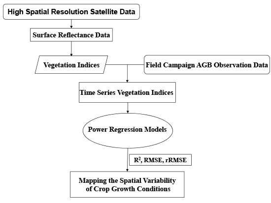However, little research has been done about the remote sensing of winter oilseed rape AGB using multiple high spatial resolution satellite data [59]. The current study dynamically mapped the winter oilseed rape growth using time series high spatial resolution satellite data for parcel-scale applications. An overall field campaign was carried out to record the AGB growth of oilseed rape, then an estimation regression model was established and validated. Eight VIs derived from the multiple high spatial resolution satellite images were used to inverse the oilseed rape AGB growth.

VIs combined with different visible and near-infrared reflectance (NIR) are significantly correlated with biomass (Table 5), and our results are consistent with previous results [43]. This is mainly due to remote sensing data that have been converted and combined into multiple VIs to minimize the variability of underlying soil, leaf angle distribution and leaf optical properties [62]. The regression models (linear, exponential, power, logarithm, and quadratic polynomial regression) have been commonly used in crop LAI and dry AGB estimation in previous studies [21,44]. A power model was found to be better than the other models in AGB estimation, demonstrating that the near-linear regression models are efficient in establishing relationships between remote sensing data and rape AGB. Estimation of crop biomass using regression models has been well demonstrated by many studies, showing that the power function model has the best accuracy [63,64,65]. A more specific reason may be the growth pattern of rapeseed AGB in this study is more similar to the power model, and that the oilseed rape AGB gradually grew at an extremely low level at the lower VI values, while quickly increasing to a maximum AGB value, at the same time the selected VIs kept increasing with a lower rate. Additionally, the waterlogging and flooding treatments reduced some AGB values, which did not result in an unpredictable sharp increase of AGB.

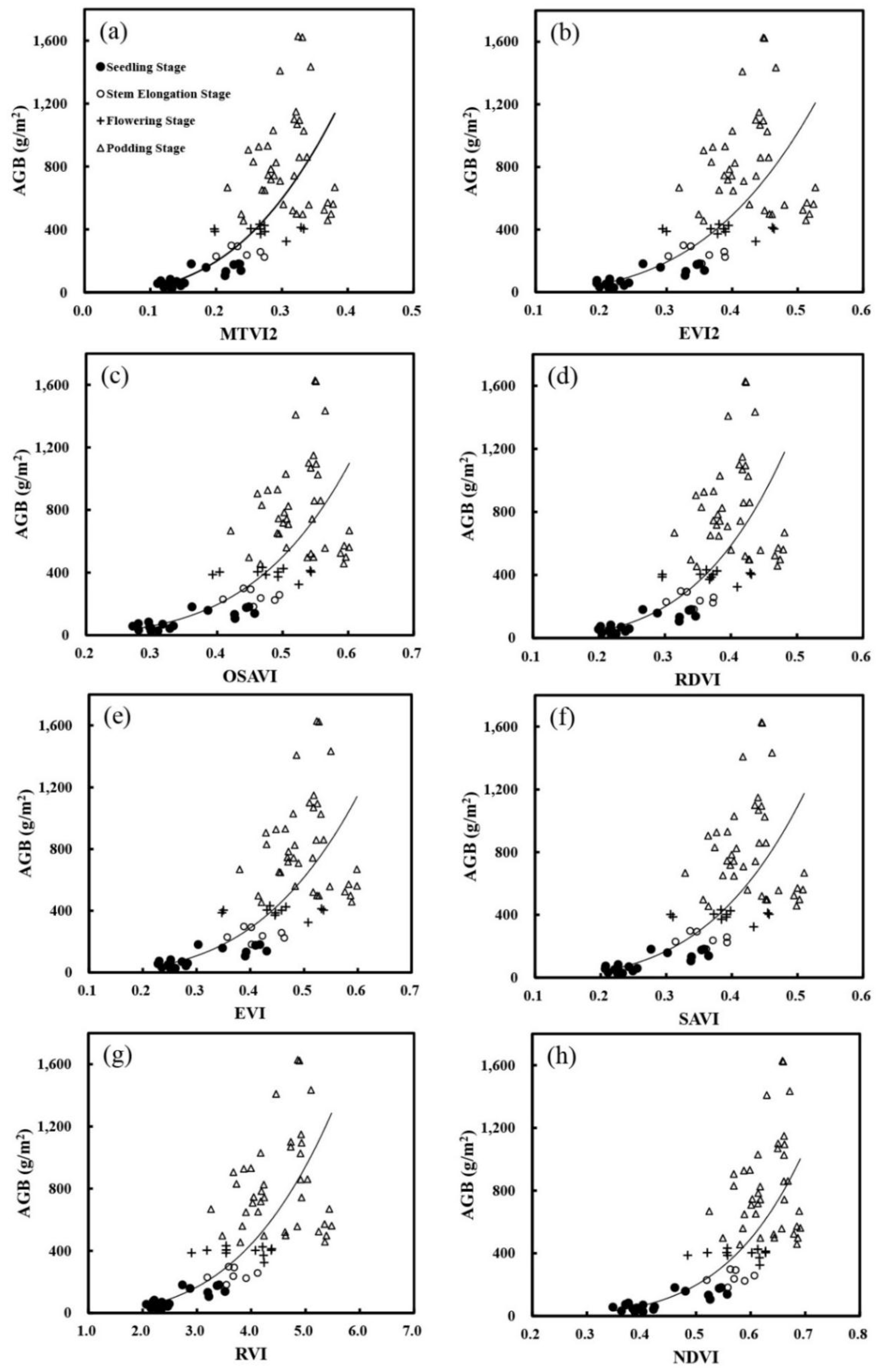
The best strategy for estimating AGB is using NDVI with a power regression model, but showed a saturation tendency of NDVI at high biomass levels. NDVI calculated from NIR and red reflectance is widely used and correlates well with LAI, fractional vegetation cover, and biomass [66]. Studies have shown that NDVI does suffer several limitations for robust estimation of biomass and a well-known reason is the saturation effect of NDVI due to the strong absorption of the red reflectance of high AGB [67]. In this study, the scatterplots in Figure 2h shows a saturation effect when NDVI is larger than 0.6, AGB becomes saturated with the AGB value, suddenly increasing from 200 g/m² to 1800 g/m². However, due to the application of waterlogging and flooding treatment, especially the flooding treatment, the treated AGB showed a declining trend compared with the contrast check group, which to a certain extent can reduce the value of the measured AGB and minimize the saturation of NDVI at high AGB. Additionally, the scatterplots also shows that at the podding stage samples were distributed away from the regression curve. In this stage, although the majority of the oilseed rape pods were green, the proportion of oilseed rape pods was high and the canopy became lager at this stage showing relatively large scattering, which may be due to the rapidly growth of the plant canopy biomass or the uncertainty of measured AGB with respect to tiny gap probabilities of the sampling. Moreover, many previous study have used NDVI time series derived from Landsat and MODIS data for forest and grassland AGB estimation [22,68].

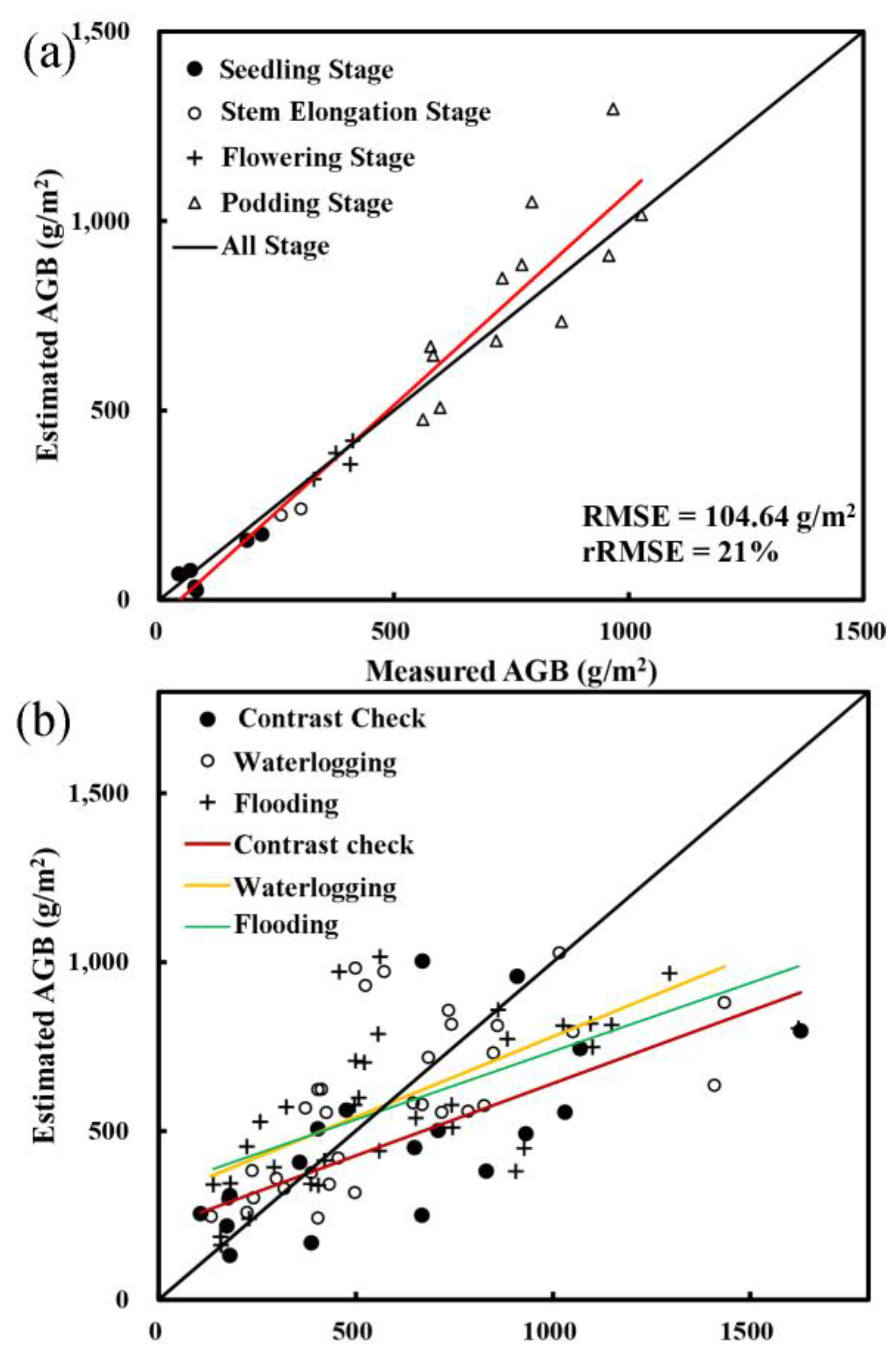
For the validation based on different soil water content treatments (Figure 3b), results disclosed that a waterlogging effect can improved the model performance for biomass estimation, mainly due to waterlogging limited crop growth, reduced the AGB value, which improved the estimation accuracy, and this is consistent with Farré‘s study [69]. Simultaneously, this may be because the NDVI gradually becomes saturated at high AGB, which shows little response to the vegetation AGB and inhibits the treatment variability measured by field campaigns [70].

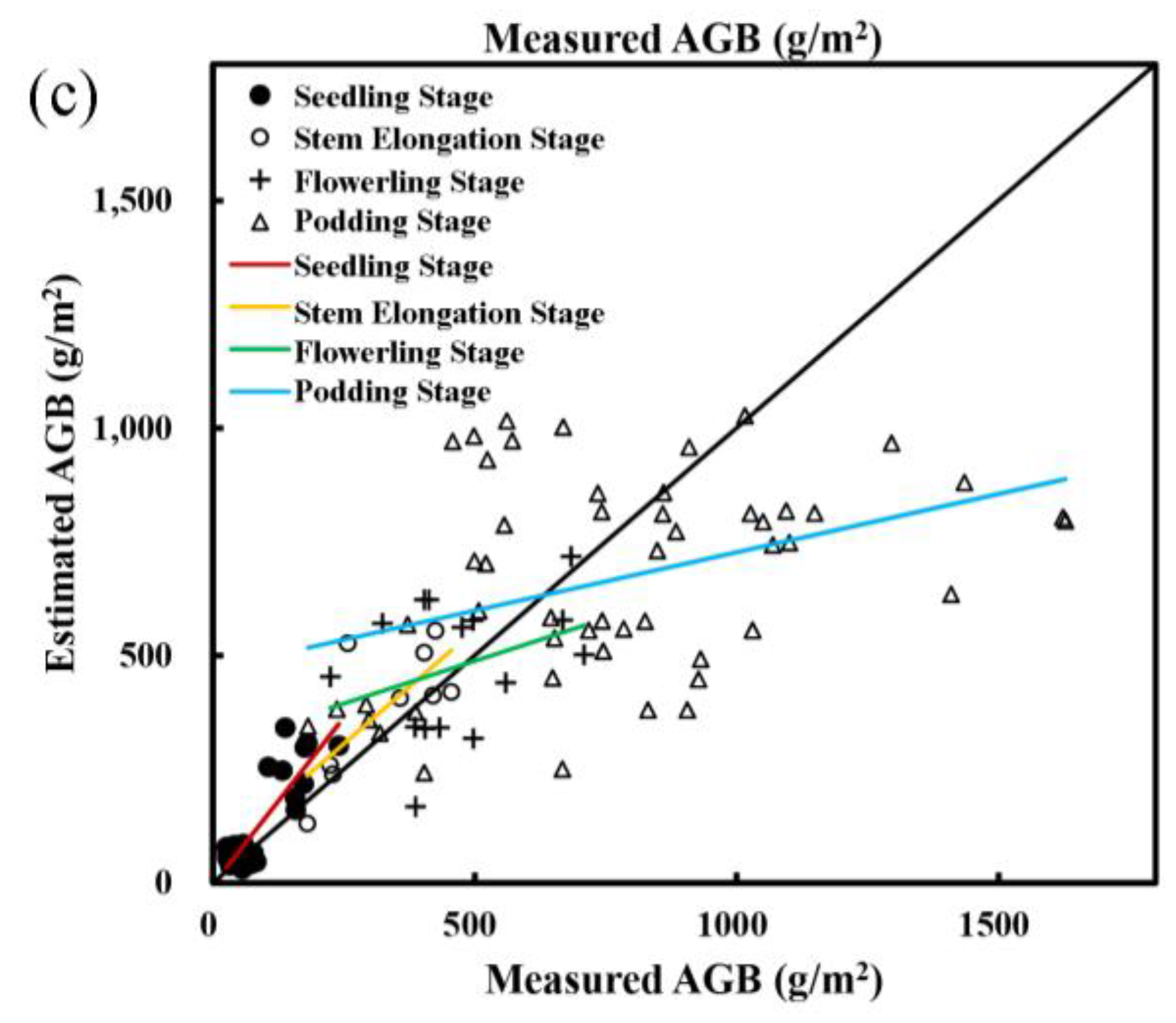
For the validation at different oilseed rape growth stages (Figure 3c), the flowering stage and podding stage apparently have greater impacts on the accuracy verification than that of the seedling stage and stem elongation stage, which may be because crop canopy structural changes and oilseed rape development are significantly correlated, especially during the growth stage from flowering to harvest [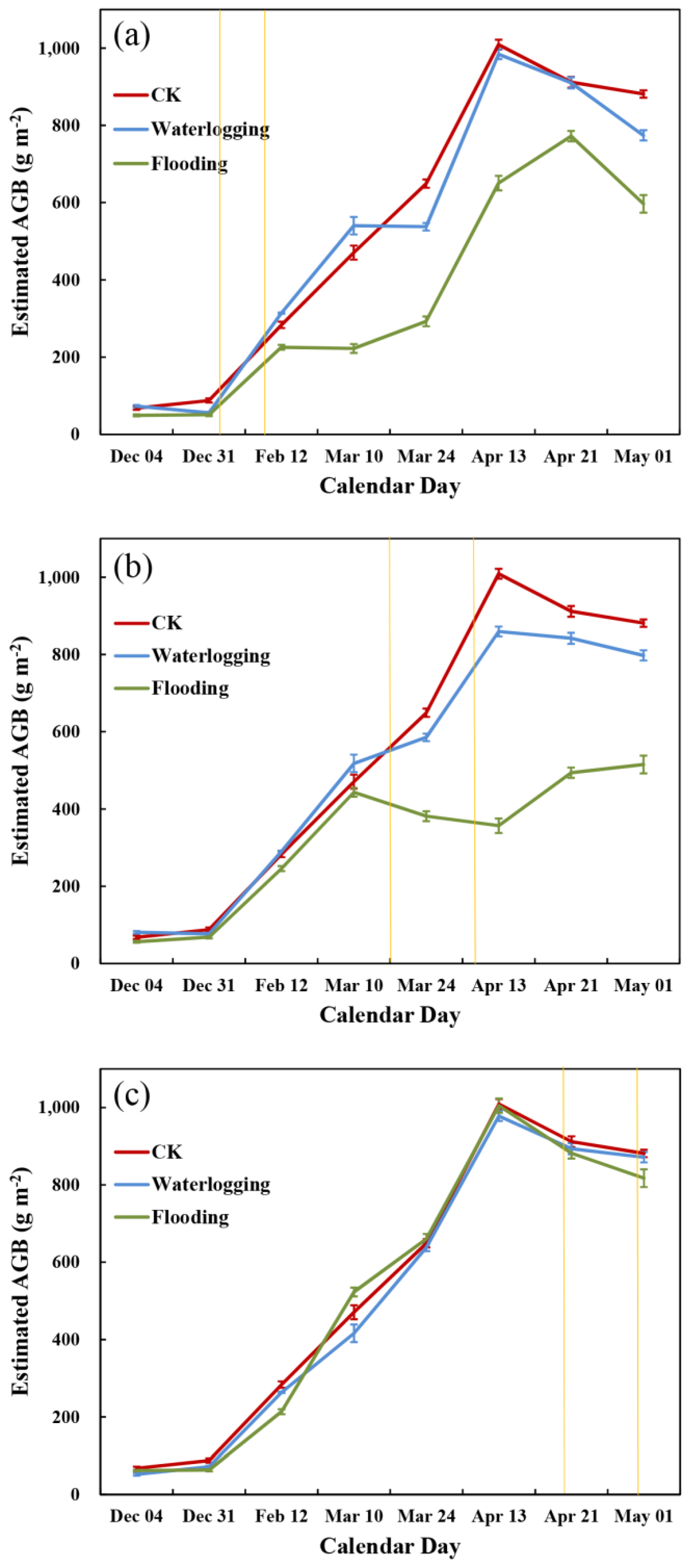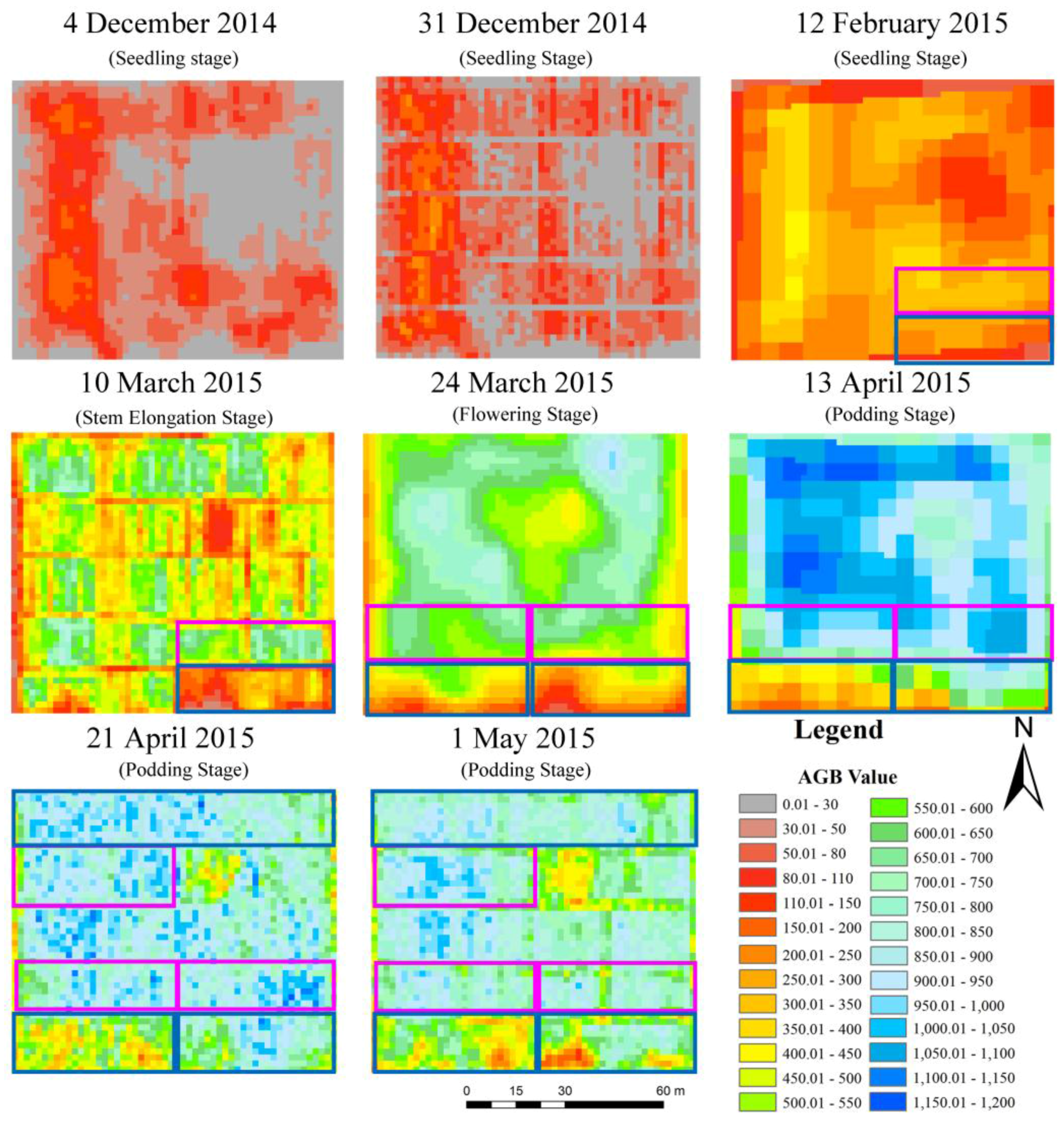71]. 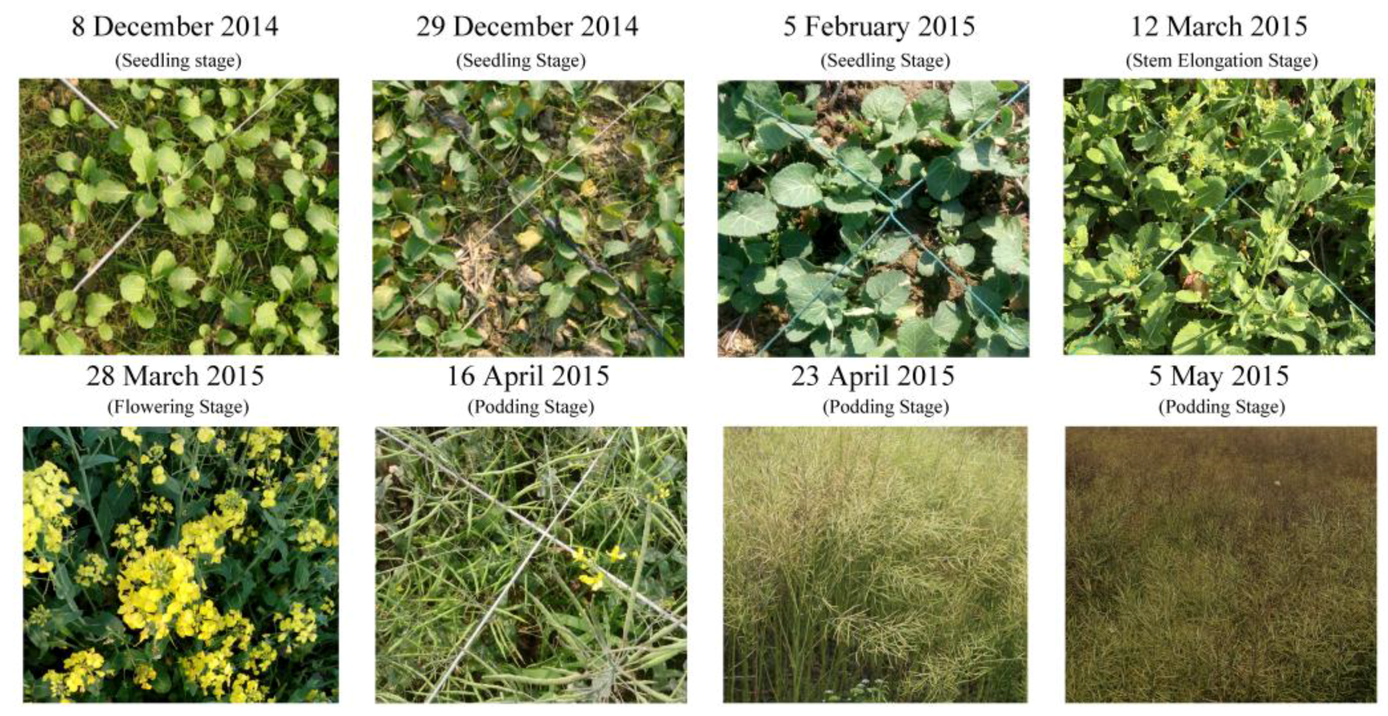Generally, winter oilseed rape biomass seasonal growth (Figure 6) developed synchronously with the dynamic maps (Figure 5) of winter oilseed rape growth. For winter oilseed rape growth, at the early growth stages (seedling stage and stem elongation stage), the soil background could have a strong influence on canopy reflectance. In addition, the rape grows slowly in the seedling stage, which mainly is a period of vegetative organ differentiation and growth. In the stem elongation stage, the main stem elongation increases rapidly, branches of stem appear constantly, and flower-bud differentiation accelerates doubly. However, at the later growth stages (flowering stage and podding stage), the estimates show a slight decrease. The main reason is that, from the beginning of flowering stage, leaf shedding causes leaves reduced drastically, which greatly reduce the photosynthetic area of the leaves, resulting in decreased chlorophyll content. However, the green leaves are still present during this period, and they develop at the lower part of the oilseed rape, under the pod. At the same time, the rapid growth of pods helps increase the assimilation area and photosynthesis. Thus, most of the plant parts that fill the field of view of the sensor are, predominantly, pods. This could be a major reason that the podding stage maps showed a different trend than the crop growth.

As for the response of crops to waterlogging, most of the previous studies put more emphasis on the impacts of waterlogging on photosynthesis and the transpiration rate, plant hormones, antioxidant enzymes, and other physiological and biochemical indices [11,13,47], and the influence of waterlogging stress on plant morphological indices, such as plant height, green leaf number, effective pod number, yield per plant, and 1000-grain weight [3,4,8,10,12]; few studies have been done on the vegetation growth and health information, such as LAI and AGB under waterlogging conditions [69,72,73]. In this study, we find that waterlogging stress can reduce the oilseed rape biomass, which has a similar consequence with previous studies [3,4,74]. After the waterlogging treatment is imposed on different oilseed rape growth stages, the response to waterlogging stress of the flowering stage was more sensitive than the seedling stage and podding stage [4], and for the same rape growth stage, the flooding treatment decreased more than the waterlogging treatment, which is consistent with previous results [3,4]. Moreover, at three different growth stages, the estimated AGB of flooding treatment continually reduced, then after a period of time it began to grow slowly, which is the performance of the flooding time-lag. However, the waterlogging treatment at the seedling stage had a better AGB value, mainly because of a severe drought condition in December 2014. These investigations showed that the selected VIs can effectively capture the growth condition under waterlogging treatment at the parcel-scale.

5. Conclusions

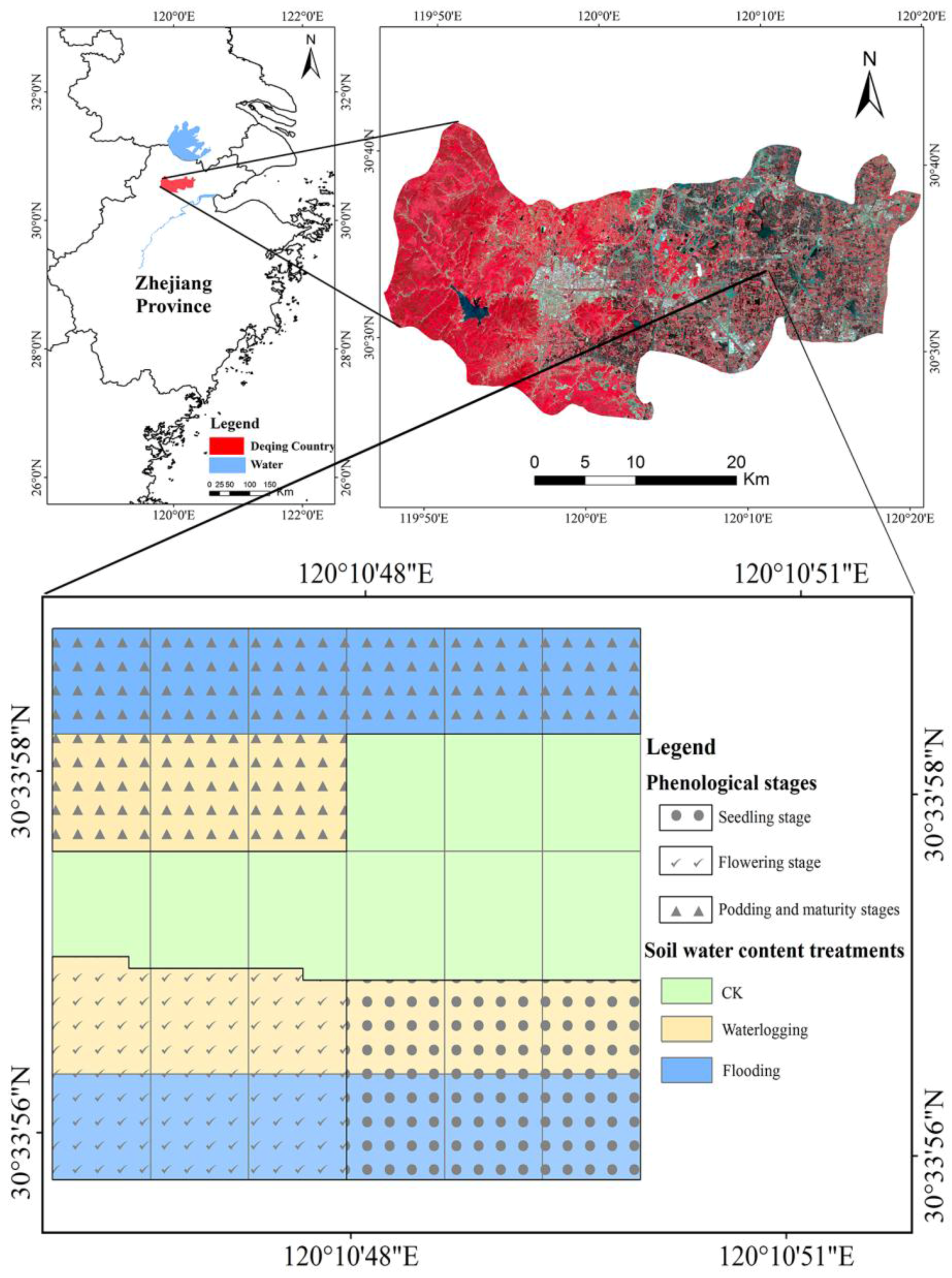
In this study, we conducted the winter oilseed rape above-ground biomass (AGB) estimates using vegetation indices (VIs) derived from multiple high spatial resolution remote sensing data. The field experiment was conducted in a consecutive rape growing season spanning from October 2014 to May 2015 by applying three different soil water content treatments (flooding, waterlogging, and contrast check) at three different growing stages (seedling stage, flowering stage, and podding stage) in the Deqing County, Southeast China. The AGB estimating equations were established between the selected VIs and the field measured AGB, and five regression models (linear, logarithmic, quadratic, power, and exponential) were examined to confirm the best empirical regression equations for estimating winter oilseed rape AGB. NDVI based on the power fit function performed better for the AGB estimation. After waterlogging stress, the oilseed rape AGB decreased, flooding treatment performed a more serious impact than waterlogging treatment, and the flowering stage is more sensitive.

This study demonstrated that high spatial resolution satellite data makes parcel-scale monitoring possible, and the multi-source high spatial resolution satellite data can be used to map the time series oilseed rape growth condition. Moreover, the remote sensing technology can capture the variability of crop AGB under waterlogging condition. As more and more high spatial resolution satellites are launched, our study could be a sign of potential application on crop growth, plant area, soil moisture, plant diseases, and insect pests, and serve the purpose of precision agriculture. The estimation of winter oilseed rape after the flowering stage using optical remote sensing data might be a challenge, and more elaborated studies are desired to further assess the property of vegetation indices across different crops, different sites, and different years.

References

1. Fu, T.D.; Tu, J.X.; Ma, C.Z.; Zhang, Y.; Zhang, D.X.; Li, X.H. The present and future of rapeseed production in china. In Proceedings of International Symposium on Rapeseed Science; Science Press: New York, NY, USA, 2001. [Google Scholar]
2. Zhang, X.K.; Chen, J.; Chen, L.; Wang, H.Z.; Li, J.N. Imbibition behavior and flooding tolerance of rapeseed seed (Brassica napus L.) with different testa color. Genet. Resour. Crop Evol. 2008, 55, 1175–1184. [Google Scholar] [CrossRef]
3. Song, F.P.; Hu, L.Y.; Zhou, G.S.; Wu, J.S.; Fu, T.D. Effects of waterlogging time on rapeseed (brassica napus l.) growth and yield. Acta Agron. Sin. 2010, 36, 170–176. [Google Scholar] [CrossRef]
4. Song, F.P.; Hu, L.Y.; Zhou, G.S.; Wu, J.S.; Fu, T.D. Effects of water table on rapeseed (Brassica napus L.) growth and yield. Acta Agrono. Sin. 2009, 35, 1508–1515. [Google Scholar] [CrossRef]
5. Xu, B.B.; Cheng, Y.; Zou, X.L.; Zhang, X.K. Ethanol content in plants of brassica napus l. Correlated with waterlogging tolerance index and regulated by lactate dehydrogenase and citrate synthase. Acta Phys. Plant 2016, 38, 1–9. [Google Scholar] [CrossRef]
6. Zou, X.L.; Hu, C.W.; Zeng, L.; Cheng, Y.; Xu, M.Y.; Zhang, X.K. A comparison of screening methods to identify waterlogging tolerance in the field in brassica napus l. During plant ontogeny. PLoS ONE 2014, 9, e89731. [Google Scholar] [CrossRef] [PubMed]
7. Hu, G.Q.; Wu, Y.Y.; Song, Z.Y.; Huang, Z.Q. The performance physiological mechanism and prevention of oliseed rape waterlogging. J. Anhui Agric. Sci. 2000, 28, 171. [Google Scholar]
8. Xu, M.Y.; Ma, H.Q.; Zeng, L.; Cheng, Y.; Lu, G.Y.; Xu, J.S.; Zhang, X.K.; Zou, X.L. The effect of waterlogging on yield and seed quality at the early flowering stage in brassica napus l. Field Crop. Res. 2015, 180, 238–245. [Google Scholar] [CrossRef]
9. Marino, S.; Cocozza, C.; Tognetti, R.; Alvino, A. Use of proximal sensing and vegetation indexes to detect the inefficient spatial allocation of drip irrigation in a spot area of tomato field crop. Precis. Agric. 2015, 16, 613–629. [Google Scholar] [CrossRef]
10. Cannell, R.Q.; Belford, R.K. Effects of waterlogging at different stages of development on the growth and yield of winter oilseed rape (Brassica napus L.). J. Sci. Food Agric. 1980, 31, 963–965. [Google Scholar] [CrossRef]
11. Zhou, W.J.; Lin, X.Q. Effects of waterlogging at different growth stages on physiological characteristics and seed yield of winter rape (Brassica napus L.). Field Crop. Res. 1995, 44, 103–110. [Google Scholar] [CrossRef]
12. Boem, F.H.G.; Lavado, R.S.; Porcelli, C.A. Note on the effects of winter and spring waterlogging on growth, chemical composition and yield of rapeseed. Field Crop. Res. 1996, 47, 175–179. [Google Scholar] [CrossRef]
13. Zhou, W.; Zhao, D.; Lin, X. Effects of waterlogging on nitrogen accumulation and alleviation of waterlogging damage by application of nitrogen fertilizer and mixtalol in winter rape (Brassica napus L.). J. Plant Growth Regul. 1997, 16, 47–53. [Google Scholar] [CrossRef]
14. Kross, A.; McNairn, H.; Lapen, D.; Sunohara, M.; Champagne, C. Assessment of rapideye vegetation indices for estimation of leaf area index and biomass in corn and soybean crops. Int. J. Appl. Earth Obs. 2015, 34, 235–248. [Google Scholar] [CrossRef]
15. Ehammer, A.; Fritsch, S.; Conrad, C.; Lamers, J.; Dech, S. Statistical derivation of fpar and lai for irrigated cotton and rice in arid uzbekistan by combining multi-temporal rapideye data and ground measurements. Proc. SPIE 2010, 7824, 782409. [Google Scholar]
16. Wang, F.M.; Huang, J.F.; Wang, Y.; Liu, Z.Y.; Peng, D.L.; Cao, F.F. Monitoring nitrogen concentration of oilseed rape from hyperspectral data using radial basis function. Int. J. Digit. Earth 2013, 6, 550–562. [Google Scholar] [CrossRef]
17. McBratney, A.; Whelan, B.; Ancev, T.; Bouma, J. Future directions of precision agriculture. Precis. Agric. 2005, 6, 7–23. [Google Scholar] [CrossRef]
18. Haboudane, D.; Miller, J.R.; Pattey, E.; Zarco-Tejada, P.J.; Strachan, I.B. Hyperspectral vegetation indices and novel algorithms for predicting green lai of crop canopies: Modeling and validation in the context of precision agriculture. Remote Sens. 2004, 90, 337–352. [Google Scholar] [CrossRef]
19. Wang, A.Q.; Chen, J.D.; Jing, C.W.; Ye, G.Q.; Wu, J.P.; Huang, Z.X.; Zhou, C.S. Monitoring the invasion of spartina alterniflora from 1993 to 2014 with landsat tm and SPOT 6 satellite data in Yueqing Bay, China. PLoS ONE 2015, 10, e0135538. [Google Scholar] [CrossRef] [PubMed]
20. Plummer, S.E. Perspectives on combining ecological process models and remotely sensed data. Ecol. Model. 2000, 129, 169–186. [Google Scholar] [CrossRef]
21. Shang, J.L.; Liu, J.G.; Huffman, T.; Qian, B.D.; Pattey, E.; Wang, J.F.; Zhao, T.; Geng, X.Y.; Kroetsch, D.; Dong, T.F.; et al. Estimating plant area index for monitoring crop growth dynamics using landsat-8 and rapideye images. J. Appl. Remote Sens. 2014, 8, 085196. [Google Scholar] [CrossRef]
22. Zhang, B.H.; Zhang, L.; Xie, D.; Yin, X.L.; Liu, C.J.; Liu, G. Application of synthetic NDVI time series blended from landsat and MODIS data for grassland biomass estimation. Remote Sens. 2015, 8, 10. [Google Scholar] [CrossRef]
23. Goetz, S.J. Multi-sensor analysis of ndvi, surface temperature and biophysical variables at a mixed grassland site. Int. J. Remote Sens. 1997, 18, 71–94. [Google Scholar] [CrossRef]
24. Huete, A.; Didan, K.; Miura, T.; Rodriguez, E.P.; Gao, X.; Ferreira, L.G. Overview of the radiometric and biophysical performance of the MODIS vegetation indices. Remote Sens. Environ. 2002, 83, 195–213. [Google Scholar] [CrossRef]
25. Bongiovanni, R.; Lowenberg-DeBoer, J. Precision agriculture and sustainability. Precis. Agric. 2004, 5, 359–387. [Google Scholar] [CrossRef]
26. Metternicht, G. Vegetation indices derived from high-resolution airborne videography for precision crop management. Int. J. Remote Sens. 2003, 24, 2855–2877. [Google Scholar] [CrossRef]
27. Thenkabail, P.S.; Stucky, N.; Griscom, B.W.; Ashton, M.S.; Diels, J.; van der Meer, B.; Enclona, E. Biomass estimations and carbon stock calculations in the oil palm plantations of african derived savannas using IKONOS data. Int. J. Remote Sens. 2004, 25, 5447–5472. [Google Scholar] [CrossRef]
28. Pu, R.; Landry, S. A comparative analysis of high spatial resolution IKONOS and Worldview-2 imagery for mapping urban tree species. Remote Sens. Environ. 2012, 124, 516–533. [Google Scholar] [CrossRef]
29. Xiong, X.X.; Lachérade, S.; Aznay, O.; Fougnie, B.; Fulbright, J.; Wang, Z.P. Comparison of S-NPP VIIRS and PLEIADES lunar observations. Proc. SPIE 2015, 9639, 96390Y. [Google Scholar]
30. Shang, J.L.; Liu, J.G.; Ma, B.L.; Zhao, T.; Jiao, X.F.; Geng, X.Y.; Huffman, T.; Kovacs, J.M.; Walters, D. Mapping spatial variability of crop growth conditions using rapideye data in Northern Ontario, Canada. Remote Sens. Environ. 2015, 168, 113–125. [Google Scholar] [CrossRef]
31. Bausch, W.C.; Khosla, R. Quickbird satellite versus ground-based multi-spectral data for estimating nitrogen status of irrigated maize. Precis. Agric. 2010, 11, 274–290. [Google Scholar] [CrossRef]
32. Huang, W.J.; Huang, J.F.; Wang, X.Z.; Wang, F.M.; Shi, J.J. Comparability of red/near-infrared reflectance and NDVI based on the spectral response function between MODIS and 30 other satellite sensors using rice canopy spectra. Sensors 2013, 13, 16023–16050. [Google Scholar] [CrossRef] [PubMed]
33. Soudani, K.; François, C.; Maire, G.; Dantec, V.L.; Dufrêne, E. Comparative analysis of IKONOS, SPOT, and ETM+ data for leaf area index estimation in temperate coniferous and deciduous forest stands. Remote Sens. Environ. 2006, 102, 161–175. [Google Scholar] [CrossRef] [Green Version]
34. Smith, K.L.; Steven, M.D.; Colls, J.J. Spectral responses of pot-grown plants to displacement of soil oxygen. Int. J. Remote Sens. 2004, 25, 4395–4410. [Google Scholar] [CrossRef]
35. Qi, J.; Chehbouni, A.; Huete, A.R.; Kerr, Y.H.; Sorooshian, S. A modified soil adjusted vegetation index. Remote Sens. 1994, 48, 119–126. [Google Scholar] [CrossRef]
36. Liu, J.G.; Pattey, E.; Miller, J.R.; McNairn, H.; Smith, A.; Hu, B.X. Estimating crop stresses, aboveground dry biomass and yield of corn using multi-temporal optical data combined with a radiation use efficiency model. Remote Sens. Environ. 2010, 114, 1167–1177. [Google Scholar] [CrossRef]
37. Cho, M.A.; Skidmore, A.; Corsi, F.; van Wieren, S.E.; Sobhan, I. Estimation of green grass/herb biomass from airborne hyperspectral imagery using spectral indices and partial least squares regression. Int. J. Appl. Earth Obs. 2007, 9, 414–424. [Google Scholar] [CrossRef]
38. Muñoz, J.D.; Finley, A.O.; Gehl, R.; Kravchenko, S. Nonlinear hierarchical models for predicting cover crop biomass using normalized difference vegetation index. Remote Sens. Environ. 2010, 114, 2833–2840. [Google Scholar] [CrossRef]
39. Huang, S.Y.; Miao, Y.X.; Zhao, G.M.; Yuan, F.; Ma, X.B.; Tan, C.X.; Yu, W.F.; Gnyp, M.L.; Lenz-Wiedemann, V.I.S.; Rascher, U.; et al. Satellite remote sensing-based in-season diagnosis of rice nitrogen status in northeast China. Remote Sens. 2015, 7, 10646–10667. [Google Scholar] [CrossRef]
40. Liu, J.G.; Pattey, E.; Jégo, G. Assessment of vegetation indices for regional crop green LAI estimation from Landsat images over multiple growing seasons. Remote Sens. Environ. 2012, 123, 347–358. [Google Scholar] [CrossRef]
41. Meroni, M.; Colombo, R.; Panigada, C. Inversion of a radiative transfer model with hyperspectral observations for LAI mapping in poplar plantations. Remote Sens. Environ. 2004, 92, 195–206. [Google Scholar] [CrossRef]
42. Hansen, P.M.; Schjoerring, J.K. Reflectance measurement of canopy biomass and nitrogen status in wheat crops using normalized difference vegetation indices and partial least squares regression. Remote Sens. Environ. 2003, 86, 542–553. [Google Scholar] [CrossRef]
43. Jin, X.L.; Yang, G.J.; Xu, X.G.; Yang, H.; Feng, H.K.; Li, Z.H.; Shen, J.X.; Zhao, C.J.; Lan, Y.B. Combined multi-temporal optical and radar parameters for estimating LAI and biomass in winter wheat using HJ and RADARSAR-2 data. Remote Sens. 2015, 7, 13251–13272. [Google Scholar] [CrossRef]
44. Gao, S.; Niu, Z.; Huang, N.; Hou, X.H. Estimating the leaf area index, height and biomass of maize using HJ-1 and RADARSAT-2. Int. J. Appl. Earth Obs. 2013, 24, 1–8. [Google Scholar] [CrossRef]
45. Gnyp, M.L.; Miao, Y.X.; Yuan, F.; Ustin, S.L.; Yu, K.; Yao, Y.K.; Huang, S.Y.; Bareth, G. Hyperspectral canopy sensing of paddy rice aboveground biomass at different growth stages. Field Crop. Res. 2014, 155, 42–55. [Google Scholar] [CrossRef]
46. Nguyen, H.T.; Lee, B.W. Assessment of rice leaf growth and nitrogen status by hyperspectral canopy reflectance and partial least square regression. Europ. J. Agronomy 2006, 24, 349–356. [Google Scholar] [CrossRef]
47. Clay, D.E.; Kim, K.I.; Chang, J.; Clay, S.A.; Dalsted, K. Characterizing water and nitrogen stress in corn using remote sensing. Agron. J. 2006, 98, 579–587. [Google Scholar] [CrossRef]
48. Li, A.; Liang, S.; Wang, A.; Qin, J. Estimating crop yield from multi-temporal satellite data using multivariate regression and neural network techniques. Photogramm. Eng. Remote Sens. 2007, 73, 1149–1157. [Google Scholar] [CrossRef]
49. Teillet, P.M.; Fedosejevs, G.; Thome, K.J.; Barker, J.L. Impacts of spectral band difference effects on radiometric cross-calibration between satellite sensors in the solar-reflective spectral domain. Remote Sens. Environ. 2007, 110, 393–409. [Google Scholar] [CrossRef]
50. Xu, J.F.; Huang, J.F. Empirical line method using spectrally stable targets to calibrate IKONOS imagery. Pedosphere 2008, 18, 124–130. [Google Scholar] [CrossRef]
51. Anaya, J.A.; Chuvieco, E.; Palacios-Orueta, A. Aboveground biomass assessment in Colombia: A remote sensing approach. For. Ecol. Manag. 2009, 257, 1237–1246. [Google Scholar] [CrossRef]
52. Jin, Y.X.; Yang, X.C.; Qiu, J.J.; Li, J.Y.; Gao, T.; Wu, Q.; Zhao, F.; Ma, H.L.; Yu, H.D.; Xu, B. Remote sensing-based biomass estimation and its spatio-temporal variations in temperate grassland, northern China. Remote Sens. 2014, 6, 1496–1513. [Google Scholar] [CrossRef]
53. Eckert, S. Improved forest biomass and carbon estimations using texture measures from Worldview-2 satellite data. Remote Sens. 2012, 4, 810–829. [Google Scholar] [CrossRef]
54. Gong, P.; Pu, R.L.; Biging, G.S.; Larrieu, M.R. Estimation of forest leaf area index using vegetation indices derived from hyperion hyperspectral data. IEEE Trans. Geosci. Remote Sens. 2003, 41, 1355–1362. [Google Scholar] [CrossRef]
55. Rondeaux, G.; Steven, M.; Baret, F. Optimization of soil-adjusted vegetation indices. Remote Sens. Environ. 1996, 55, 95–107. [Google Scholar] [CrossRef]
56. Baret, F.; Guyot, G. Potentials and limits of vegetation indices for LAI and APAR assessment. Remote Sens. Environ. 1991, 35, 161–173. [Google Scholar] [CrossRef]
57. Eitel, J.U.H.; Long, D.S.; Gessler, P.E.; Hunt, E.R. Combined spectral index to improve ground-based estimates of nitrogen status in dryland wheat. Agron. J. 2008, 100, 1694. [Google Scholar] [CrossRef]
58. Clevers, J.G.P.W.; van der Heijden, G.W.A.M.; Verzakov, S.; Schaepman, M.E. Estimating grassland biomass using SVM band shaving of hyperspectral data. Photogramm. Eng. Remote Sens. 2007, 73, 1141–1148. [Google Scholar] [CrossRef]
59. Cheng, Q. Validation and correction of MOD15-LAI using in situ rice LAI in southern China. Commun. Soil Sci. Plant Anal. 2008, 39, 1658–1669. [Google Scholar] [CrossRef]
60. Battude, M.; Al Bitar, A.; Morin, D.; Cros, J.; Huc, M.; Marais Sicre, C.; Le Dantec, V.; Demarez, V. Estimating maize biomass and yield over large areas using high spatial and temporal resolution Sentinel-2 like remote sensing data. Remote Sens. 2016, 184, 668–681. [Google Scholar] [CrossRef]
61. Sakowska, K.; Juszczak, R.; Gianelle, D. Remote sensing of grassland biophysical parameters in the context of the Sentinel-2 satellite mission. J. Sens. 2016, 2016, 1–16. [Google Scholar] [CrossRef]
62. Darvishzadeh, R.; Skidmore, A.; Atzberger, C.; Wieren, S. Estimation of vegetation lai from hyperspectral reflectance data: Effects of soil type and plant architecture. Int. J. Appl. Earth Obs. 2008, 10, 358–373. [Google Scholar] [CrossRef]
63. Ma, B.L.; Dwyer, L.M.; Costa, C.; Cober, E.R.; Morrison, M.J. Early prediction of soybean yield from canopy reflectance measurements. Agron. J. 2001, 93, 1227–1234. [Google Scholar] [CrossRef]
64. Carter, G.A.; Spiering, B.A. Optical properties of intact leaves for estimating chlorophyll concentration. J. Environ. Qual. 2002, 31, 1424–1432. [Google Scholar] [CrossRef] [PubMed]
65. Suganuma, H.; Abe, Y.; Taniguchi, M.; Tanouchi, H.; Utsugi, H.; Kojima, T.; Yamada, K. Stand biomass estimation method by canopy coverage for application to remote sensing in an arid area of Western Australia. For. Ecol. Manag. 2006, 222, 75–87. [Google Scholar] [CrossRef]
66. Carlson, T.N.; Riziley, D.A. On the relation between NDVI, fractional vegetation cover, and leaf area index. Remote Sens. Environ. 1997, 62, 241–252. [Google Scholar] [CrossRef]
67. Tian, F.; Brandt, M.; Liu, Y.Y.; Verger, A.; Tagesson, T.; Diouf, A.A.; Rasmussen, K.; Mbow, C.; Wang, Y.; Fensholt, R. Remote sensing of vegetation dynamics in drylands: Evaluating vegetation optical depth (VOD) using AVHRR NDVI and in situ green biomass data over West African Sahel. Remote Sens. 2016, 177, 265–276. [Google Scholar] [CrossRef]
68. Zhu, X.L.; Liu, D.S. Improving forest aboveground biomass estimation using seasonal Landsat NDVI time-series. ISPRS J. Photogramm. 2015, 102, 222–231. [Google Scholar] [CrossRef]
69. Farré, I.; Robertson, M.J.; Asseng, S.; French, R.; Dracup, M. Simulating lupin development, growth, and yield in a Mediterranean environment. Crop Pasture Sci. 2004, 55, 863–877. [Google Scholar] [CrossRef]
70. Gitelson, A.A. Wide dynamic range vegetation index for remote quantification of biophysical characteristics of vegetation. J. Plant Physiol. 2004, 161, 165–173. [Google Scholar] [CrossRef] [PubMed]
71. Fritsch, S.; Machwitz, M.; Ehammer, A.; Conrad, C.; Dech, S. Validation of the collection 5 MODIS FPAR product in a heterogeneous agricultural landscape in arid Uzbekistan using multitemporal RapidEye imagery. Int. J. Remote Sens 2012, 33, 6818–6837. [Google Scholar] [CrossRef]
72. Smethurst, C.F.; Shabala, S. Screening methods for waterlogging tolerance in lucerne: Comparative analysis of waterlogging effects on chlorophyll fluorescence, photosynthesis, biomass and chlorophyll content. Funct. Plant Biol. 2003, 30, 335–343. [Google Scholar] [CrossRef]
73. Rubio, G.; Casasola, G.; Lavado, R.S. Adaptations and biomass production of two grasses in response to waterlogging and soil nutrient enrichment. Oecologia 1995, 102, 102–105. [Google Scholar] [CrossRef]
74. Wang, N.; Yu, F.H.; Li, P.X.; He, W.M.; Liu, J.; Yu, G.L.; Song, Y.B.; Dong, M. Clonal integration supports the expansion from terrestrial to aquatic environments of the amphibious stoloniferous herb alternanthera philoxeroides. Plant Biol. 2009, 11, 483–489. [Google Scholar] [CrossRef] [PubMed]
Figure 1. Experiments designed from October 2014 to May 2015 at the Deqing study site, Zhejiang, China. Background maps were color composite GF-1 acquired on 12 May 2015, with the (RGB) band combination= bands 4, 3, 2.
Remotesensing 09 00238 g001
Figure 2. Scatter plots showing the relationships between the selected vegetation indices (VIs) and above ground biomass (AGB) of winter oilseed rape from October 2014 to May 2015 for (a) MTVI2; (b) EVI2; (c) OSAVI; (d) RDVI; (e) EVI; (f) SAVI; (g) RVI; and (h) NDVI; the data set used to establish the regression model is the calibration set; the power regression lines are also shown.
Remotesensing 09 00238 g002
Figure 3. Comparison between measured AGB and estimated AGB. The black dash line is the 1:1 line and the colorized solid lines are the linear regression trend lines. The data set we used were: (a) the validation set; (b) the data collected from the plots conducting, or had finished with, the soil water content stress treatments; (c) the data collected from different growth stages.
Remotesensing 09 00238 g003aRemotesensing 09 00238 g003b
Figure 4. Variation of the estimated AGB for different soil water content treatments from 2014 to 2015 growth stages. (ac) represents the soil water content treatments imposed at seedling stage, flowering stage, and podding stage, respectively. The shallow orange vertical lines mean the date of waterlogging treatments imposed at three growth stages, respectively.
Remotesensing 09 00238 g004
Figure 5. Maps of winter oilseed rape AGB during the vegetative growth stages from 2014 to 2015. The blue rectangles and red rectangles represent the plots were conducting, or had finished with, the flooding and waterlogging treatment, respectively.
Remotesensing 09 00238 g005
Figure 6. Winter oilseed rape seasonal growth from 2014 to 2015.
Remotesensing 09 00238 g006