
A Lookup Table-Based Method for Estimating Sea Surface Hemispherical Broadband Emissivity Values (8–13.5 μm)


Abstract
:1. Introduction
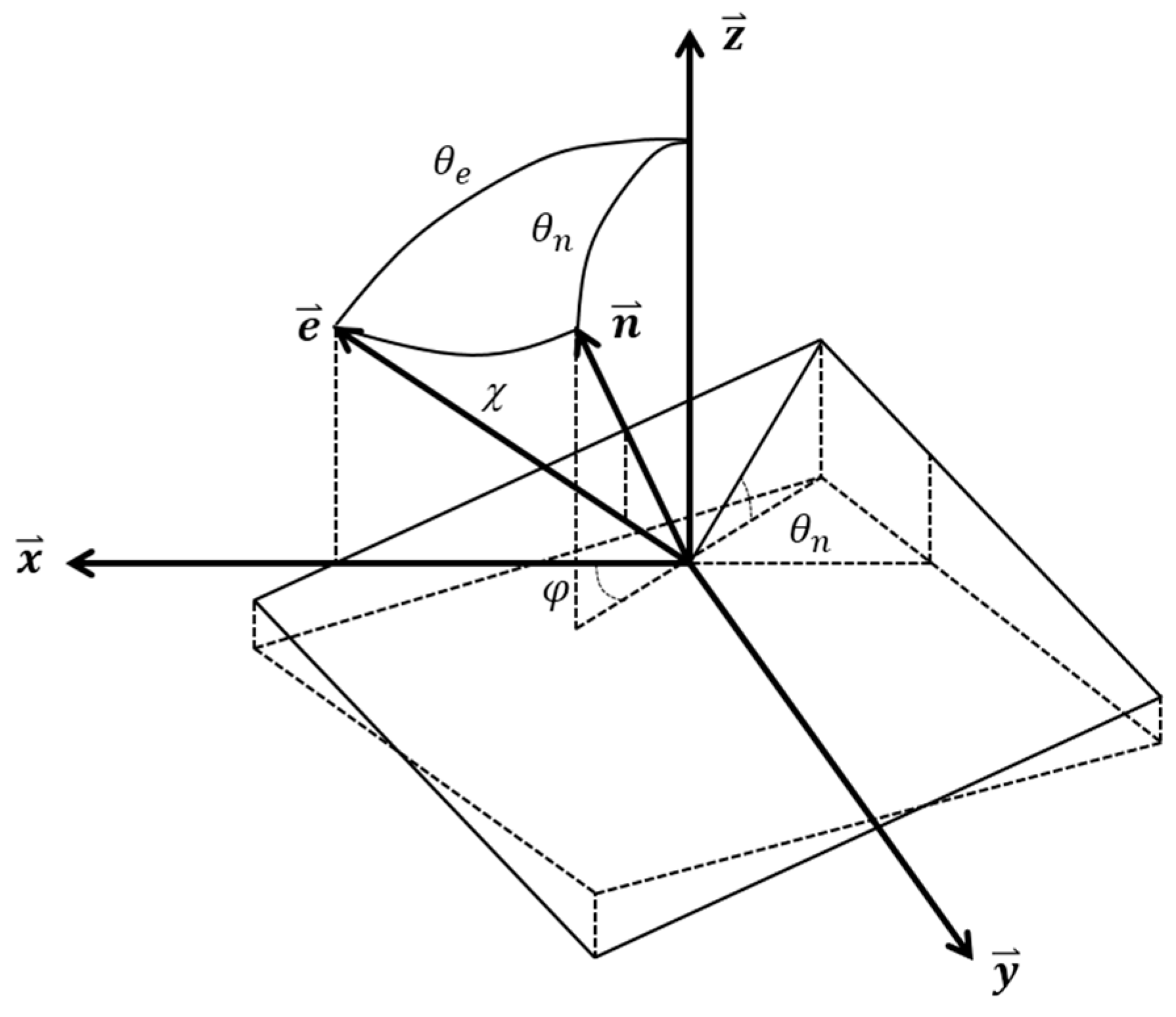
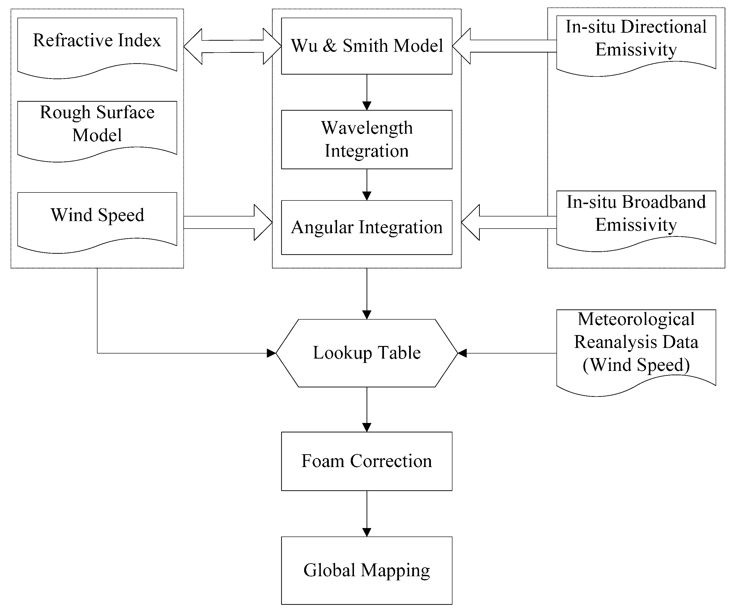
2. Data and Methods
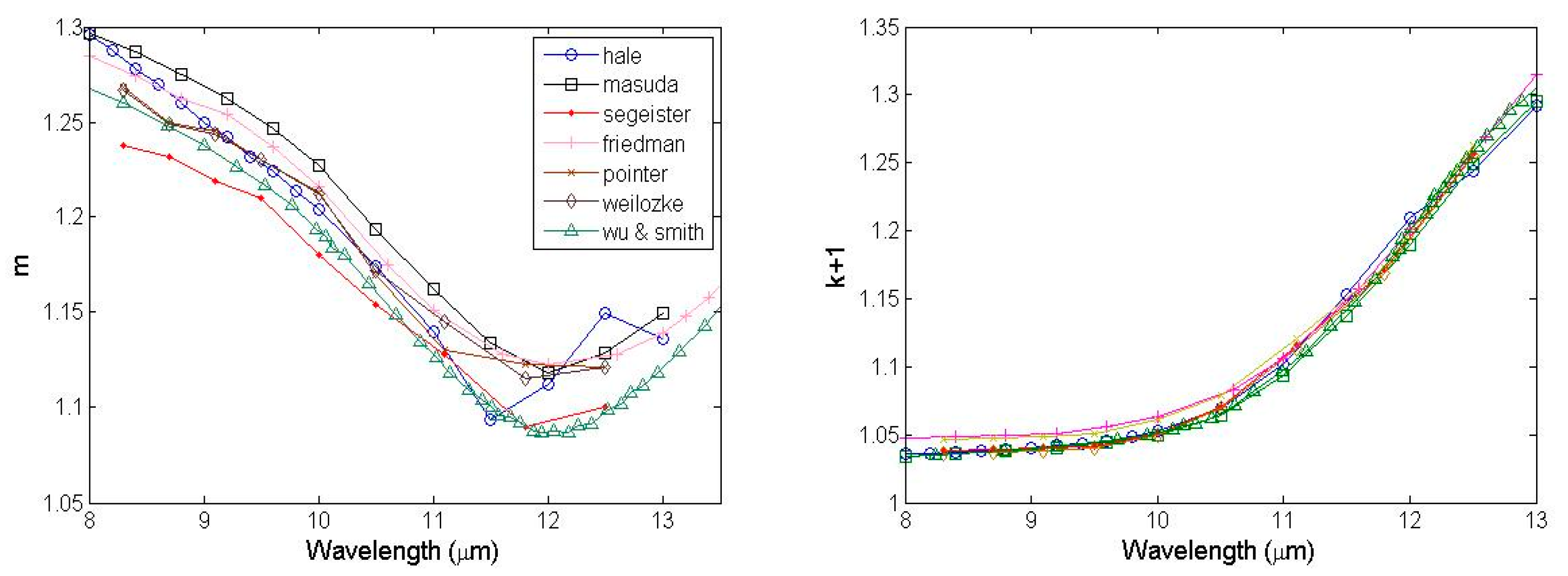
2.1. Refractive Index
2.2. In Situ Measurements
2.3. Meteorological Reanalysis Data
2.4. Wu and Smith Model
2.5. Description of Our Method
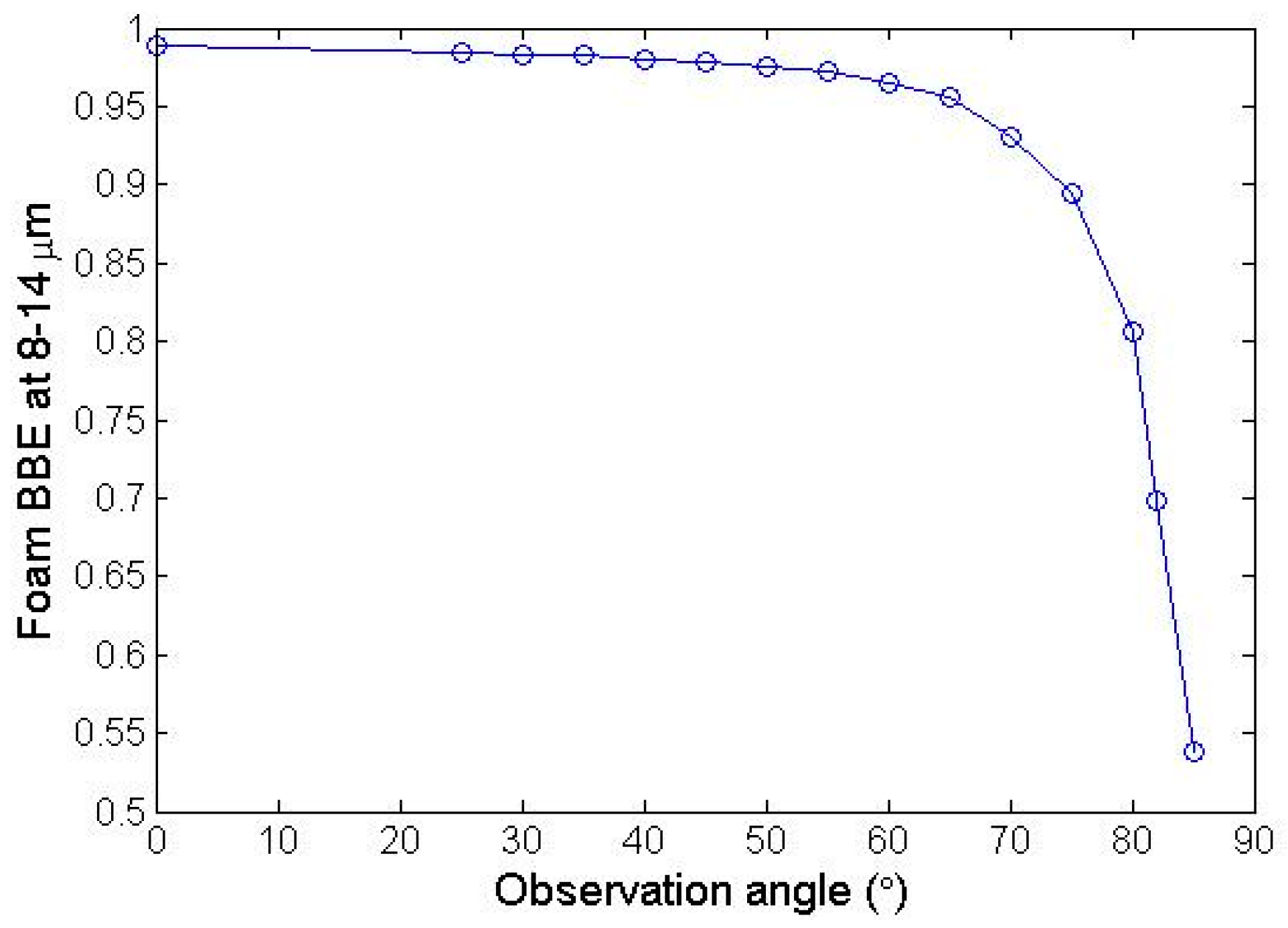
3. Analysis of the Results
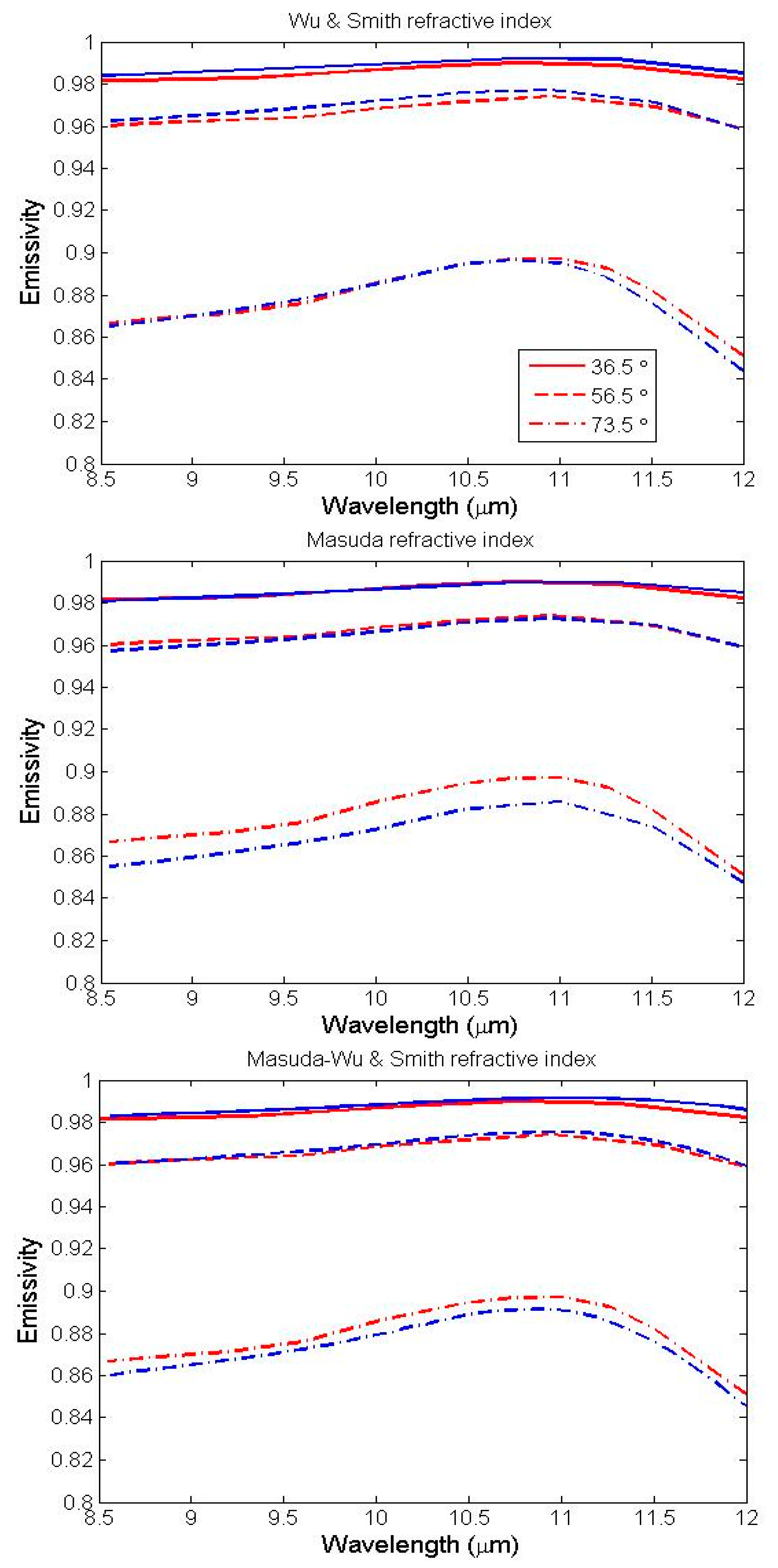
3.1. Determining Optimal Sea Water Optical Constants
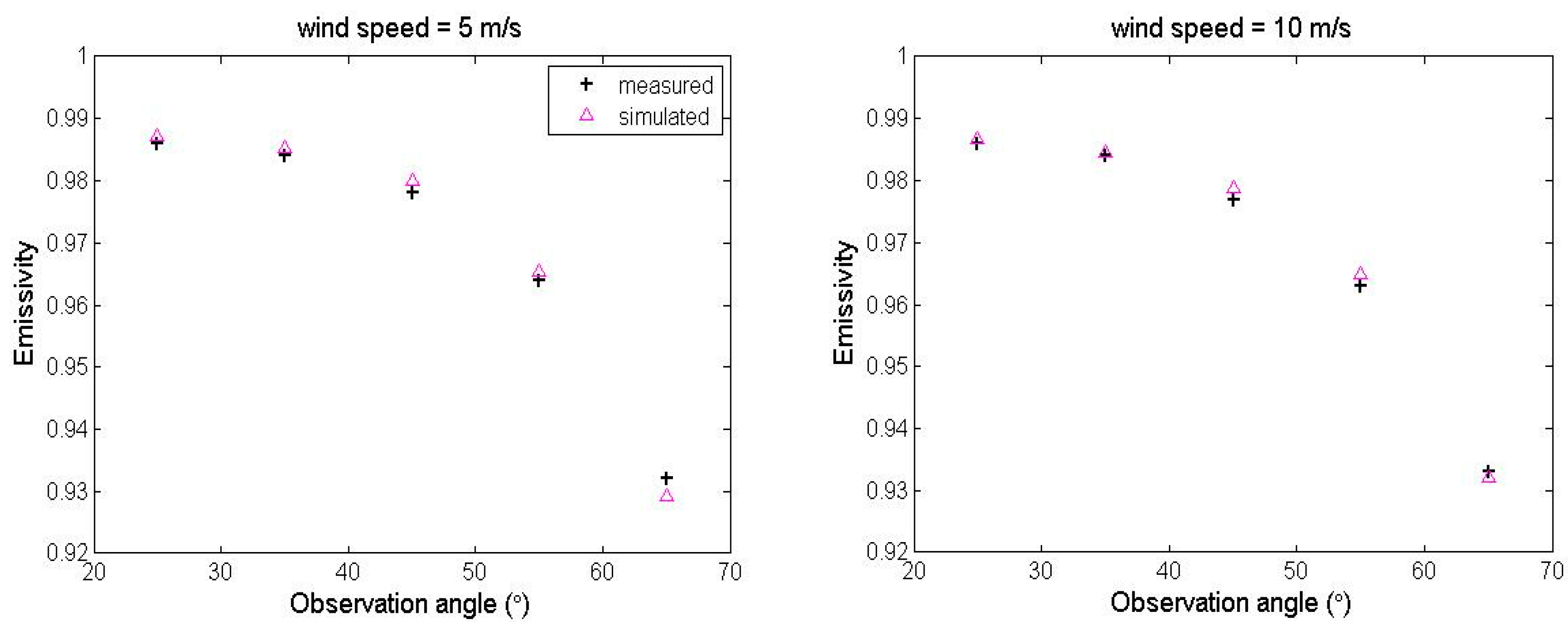
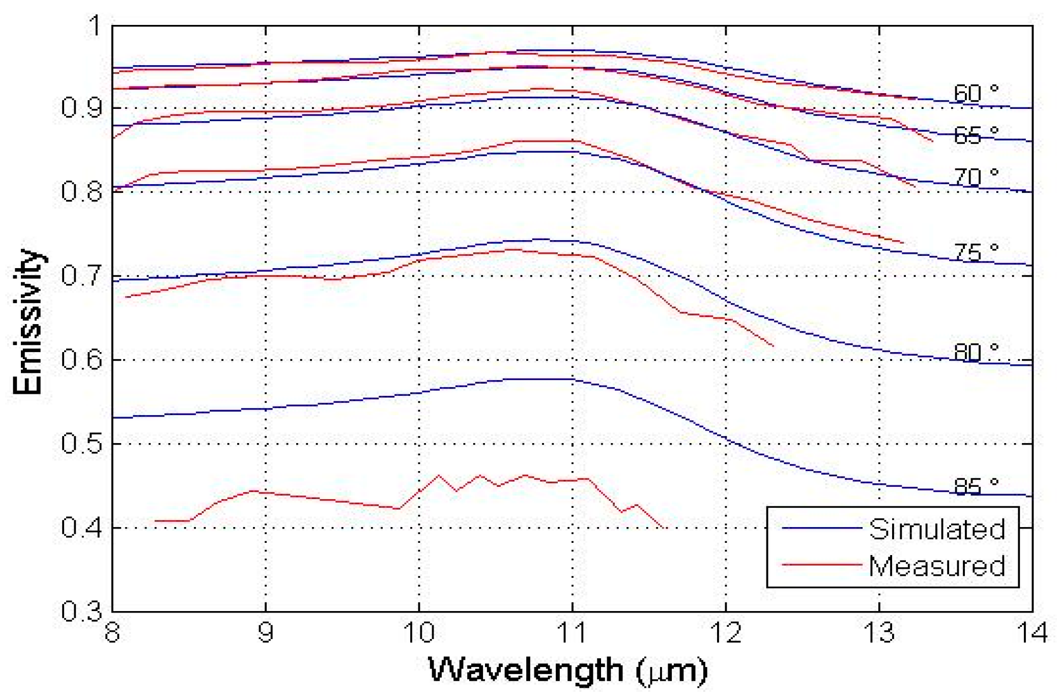
3.2. Validation of the Simulated Directional and Hemispherical BBE
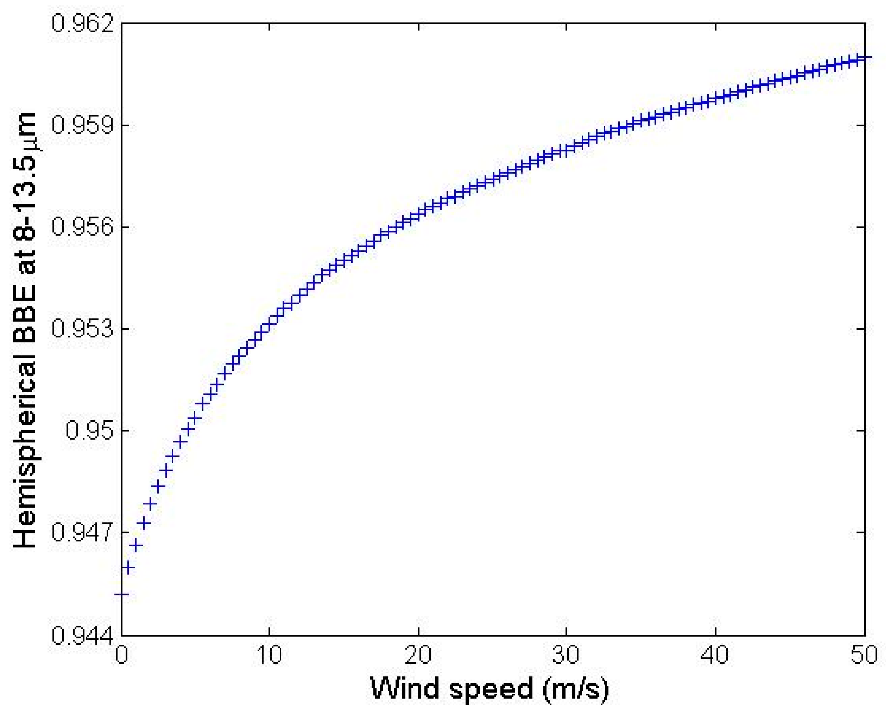
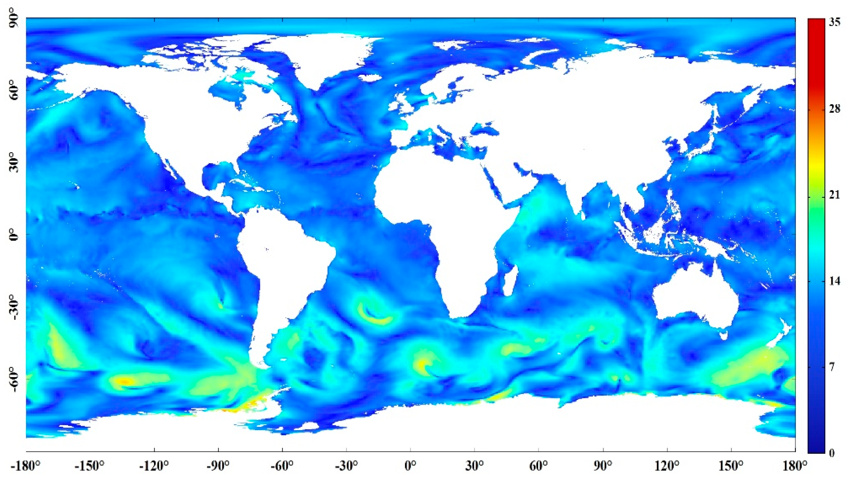
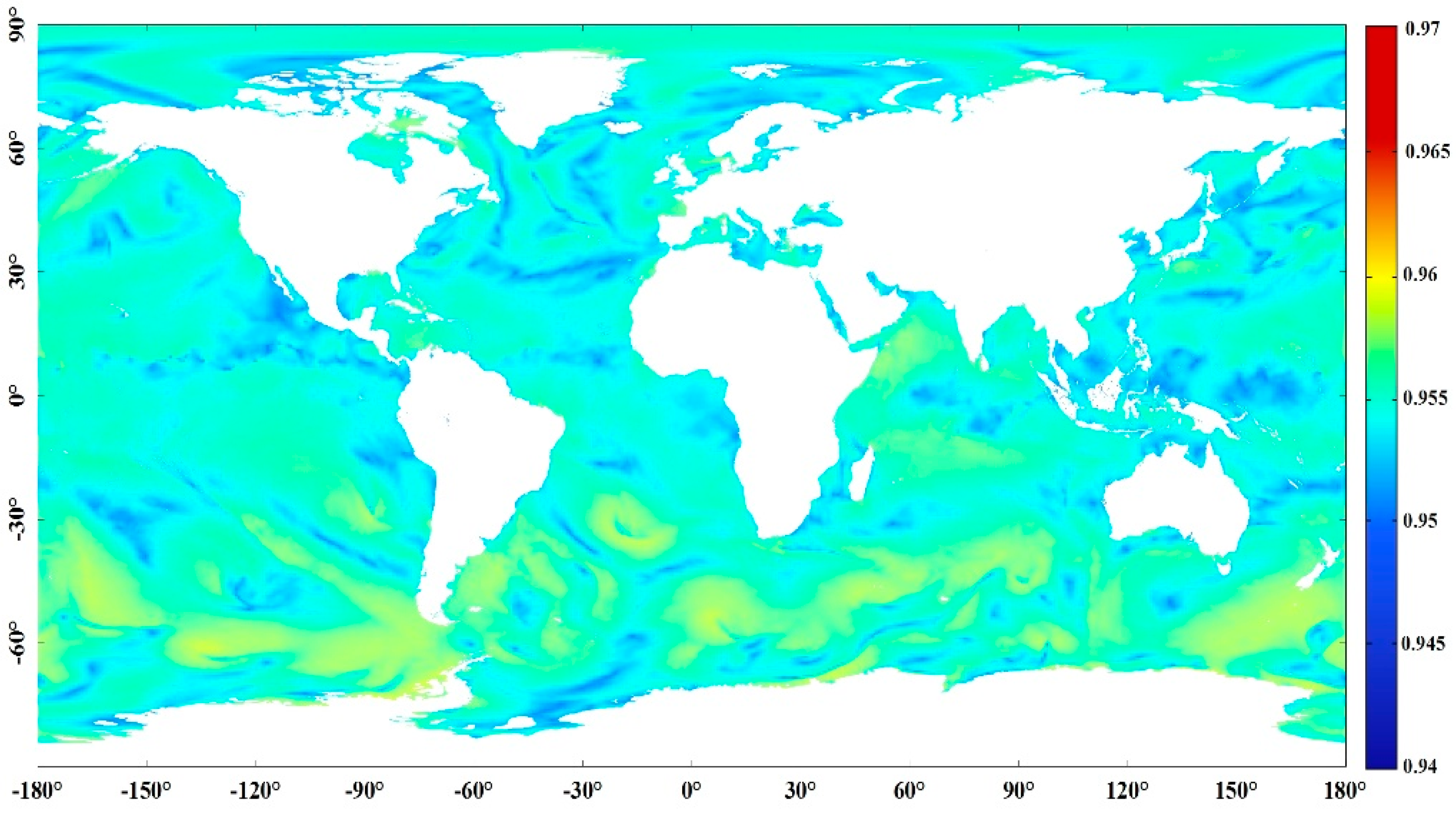
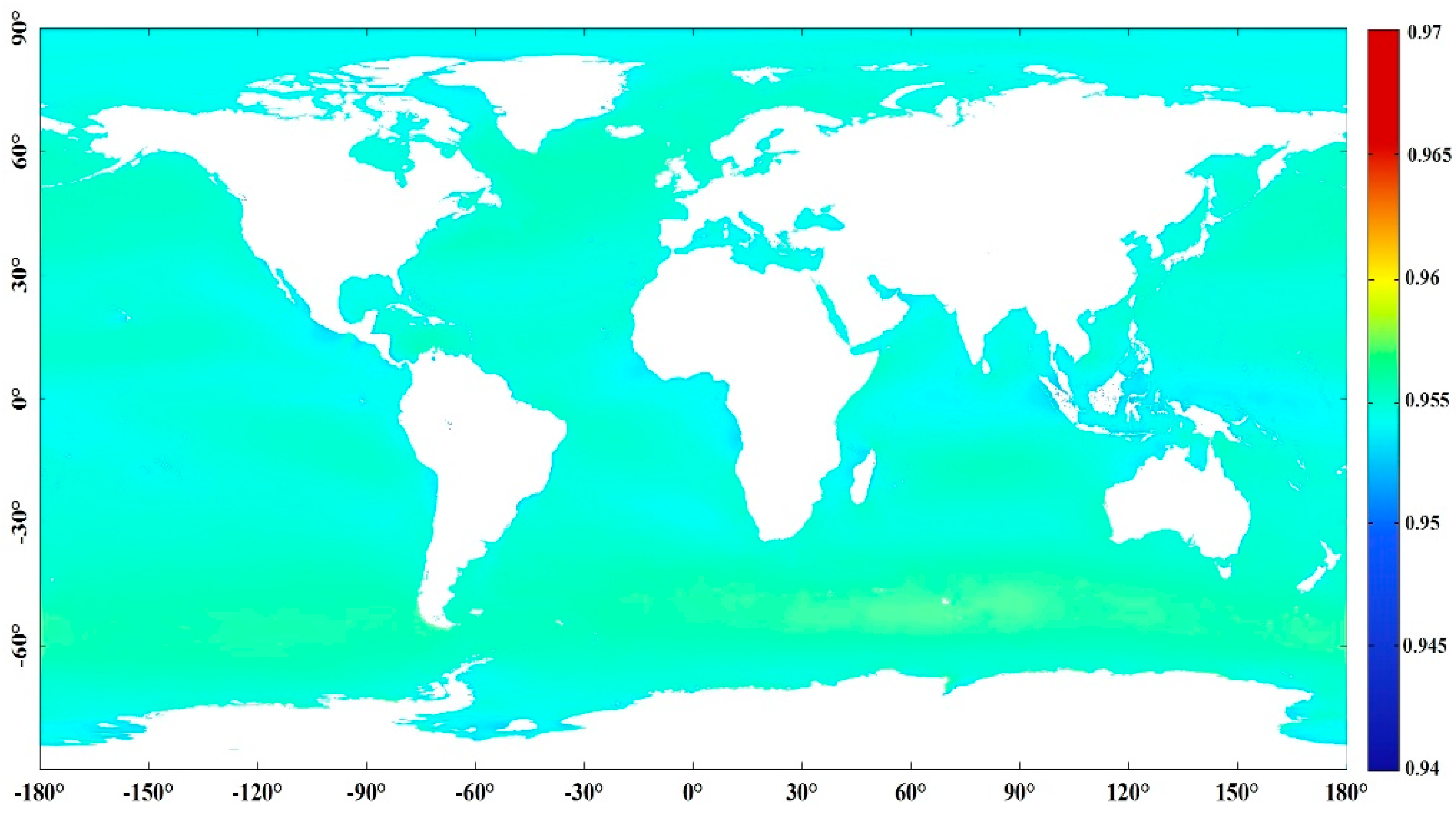
3.3. Mapping Global Ocean Hemispherical BBE
4. Discussion
5. Conclusions
Acknowledgments
Author Contributions
Conflicts of Interest
References
- McMillin, L.M. Estimation of sea surface temperature from two infrared window measurements with different absorption. J. Geophys. Res. 1975, 20, 11587–11601. [Google Scholar] [CrossRef]
- Niclos, R.; Estrela, M.J.; Valiente, J.A.; Barbera, M.J. Proposal and validation of an emissivity-dependent algorithm to retrieve sea-surface temperature from MSG-SEVIRI data. IEEE Geosci. Remote Sens. Lett. 2010, 7, 786–790. [Google Scholar] [CrossRef]
- Barton, I.J. Satellite-derived sea surface temperatures—A comparison between operational, theoretical and experimental algorithms. J. Appl. Meteorol. 1992, 31, 432–442. [Google Scholar] [CrossRef]
- Kilpatrick, K.A.; Podesta, G.; Walsh, S.; Williams, E.; Halliwell, V.; Szczodrak, M.; Brown, O.B.; Minnett, P.J.; Evans, R. A decade of sea surface temperature from modis. Remote Sens. Environ. 2015, 165, 27–41. [Google Scholar] [CrossRef]
- Niclos, R.; Caselles, V.; Coll, C.; Valor, E. Determination of sea surface temperature at large observation angles using an angular and emissivity dependent split-window equation. Remote Sens. Environ. 2007, 111, 107–121. [Google Scholar] [CrossRef]
- Hanafin, J.A.; Minnett, P.J. Measurements of the infrared emissivity of a wind-roughened sea surface. Appl. Opt. 2005, 44, 398–411. [Google Scholar] [CrossRef] [PubMed]
- Wu, X.; Smith, W.L. Sensitivity of sea surface temperature retrieval to sea surface emissivity. ACTA Meteorol. Sin. 1996, 10, 376–384. [Google Scholar]
- Von Schuckmann, K.; Palmer, M.D.; Trenberth, K.E.; Cazenave, A.; Chambers, D.; Champollion, N.; Hansen, J.; Josey, S.A.; Leob, N.; Mathieu, P.-P.; et al. An imperative to monitor earth’s energy imbalance. Nat. Clim. Chang. 2016, 6, 138–144. [Google Scholar] [CrossRef]
- Trenberth, K.E.; Fasullo, J.T.; Balmaseda, M.A. Earth’s energy imbalance. J. Clim. 2014, 27, 3129–3144. [Google Scholar] [CrossRef]
- Stephens, G.L.; L’Ecuyer, T. The earth’s energy balance. Atmos. Res. 2015, 166, 195–203. [Google Scholar] [CrossRef]
- Cheng, J.; Liang, S.; Yao, Y.; Zhang, X. Estimating the optimal broadband emissivity spectral range for calculating surface longwave net radiation. IEEE Geosci. Remote Sens. Lett. 2013, 10, 401–405. [Google Scholar] [CrossRef]
- Cheng, J.; Liang, S. Effects of thermal-infrared emissivity directionality on surface broadband emissivity and longwave net radiation estimation. IEEE Geosci. Remote Sens. Lett. 2014, 11, 499–503. [Google Scholar] [CrossRef]
- Masuda, K.; Takashima, T.; Takayama, Y. Emissivity of pure and sea waters for the model sea surface in the infrared window regions. Remote Sens. Environ. 1988, 24, 313–329. [Google Scholar] [CrossRef]
- Cox, C.; Munk, W. Statistics of the sea surface derived from sun glitter. J. Mar. Res. 1954, 13, 198–227. [Google Scholar]
- Watts, P.D.; Allen, M.R.; Nightingale, T.J. Wind speed effects on sea surface emission and reflection for the along track scanning radiometer. J. Atmos. Ocean. Technol. 1996, 13, 126–141. [Google Scholar] [CrossRef]
- Wu, X.; Smith, W.L. Emissivity of rough sea surface for 8–13 um: Modeling and verification. Appl. Opt. 1997, 36, 2609–2619. [Google Scholar] [CrossRef] [PubMed]
- Masuda, K. Infrared sea surface emissivity including multiple reflection effect for isotropic Gaussian slope distripution model. Remote Sens. Environ. 2006, 103, 488–496. [Google Scholar] [CrossRef]
- Freund, D.E.; Joseph, R.I.; Donohue, D.J.; Constantikes, K.T. Numerical computations of rough sea surface emissivity using the interaction probability density. J. Opt. Soc. Am. A 1997, 14, 1836–1849. [Google Scholar] [CrossRef]
- Henderson, B.G.; Theiler, J.; Villeneuve, P. The polarized emissivity of a wind-roughened sea surface: A monte carlo model. Remote Sens. Environ. 2003, 88, 453–467. [Google Scholar] [CrossRef]
- Nalli, N.R.; Minnett, P.J.; delst, P.V. Emissivity and reflection model for calculating unpolarized isotropic water surface-leaving radiance in the infrared. I. Theoretical development and calculations. Appl. Opt. 2008, 47, 3701–3721. [Google Scholar] [CrossRef] [PubMed]
- Nalli, N.R.; Minnett, P.J.; Maddy, E.; McMillan, W.W.; Goldberg, M.D. Emissivity and reflection model for calculating unpolarized isotropic water surface-leaving radiance in the infrared. 2: Validation using fourier transform spectrometers. Appl. Opt. 2008, 47, 4649–4671. [Google Scholar] [CrossRef] [PubMed]
- Van Delst, P. JCSDA infrared sea surface emissivity model. In Proceedings of the 13th International TOVS Study Conference, Sainte-Adele, QC, Canada, 29 October–4 November 2003.
- Hale, G.M.; Querry, M.R. Optical constants of water in the 200-nm to 200-um wavelength region. Appl. Opt. 1973, 12, 555–563. [Google Scholar] [CrossRef] [PubMed]
- Friedman, D. Infrared characteristics of ocean water (1.5–15 microns). Appl. Opt. 1969, 8, 2073–2078. [Google Scholar] [CrossRef] [PubMed]
- Pointer, L.; Dechambenoy, C. Determination des constantes optiques del’eau entre 1 et 40 um. Ann. Geophys. 1966, 22, 633–641. [Google Scholar]
- Wieliczka, D.M.; Weng, S.; Querry, M.R. Wedge shaped cell for highly absorbent liquids: Infrared optical constants of water. Appl. Opt. 1989, 28, 1714–1719. [Google Scholar] [CrossRef] [PubMed]
- Niclos, R.; Caselles, V.; Valor, E.; Coll, C.; Sanchez, J.M. A simple equation for determining sea surface emissivity in the 3-15 um. Int. J. Remote Sens. 2009, 30, 1603–1619. [Google Scholar] [CrossRef]
- Smith, W.L.; Knuteson, R.O.; Revercomb, H.E.; Feltz, W.; Howell, H.B.; Menzel, W.P.; Nalli, N.; Brown, O.B.; Minnett, P.J.; McKeown, W. Observations of the infrared radiative properties of the ocean—Implications for the measurement of sea surface temperature via satellite remote sensing. Bull. Am. Meteorol. Soc. 1996, 77, 41–51. [Google Scholar] [CrossRef]
- Niclos, R.; Valor, E.; Caselles, V.; Coll, C.; Sanchez, J.M. In situ angular measurements of thermal infrared sea surface emissivity—Validation of models. Remote Sens. Environ. 2005, 94, 83–93. [Google Scholar] [CrossRef]
- Niclos, R.; Caselles, V.; Coll, C.; Valor, E.; Rubio, E. Autonomous measurements of sea surface temperature using in situ thermal infrared data. J. Atmos. Ocean. Tech. 2004, 21, 683–692. [Google Scholar] [CrossRef]
- Niclos, R.; Dona, C.; Valor, E.; Bisquert, M. Thermal-infrared spectral and angular characterization of crude oil and seawater emissivities for oil slick identification. IEEE Trans. Geosci. Remote Sens. 2014, 52, 5387–5395. [Google Scholar] [CrossRef]
- Niclos, R.; Caselles, V.; Valor, E.; Coll, C. Foam effect on the sea surface emissivity in the 8–14 um region. J. Geophys. Res. 2007, 112. [Google Scholar] [CrossRef]
- Branch, R.; Chickadel, C.C.; Jessup, A.T. Infrared emissivity of seawater and foam at large incidence angles in the 3–14 um wavelength range. Remote Sens. Environ. 2016, 184, 15–24. [Google Scholar] [CrossRef]
- Ogawa, K.; Schmugge, T.; Jacob, F.; Prench, A. Estimation of broadband land surface emissivity from multi-spectral thermal infrared remote sensing. Agronomie 2002, 22, 695–696. [Google Scholar] [CrossRef]
- Hapke, B. Theory of Reflectance and Emittance Spectroscopy; Cambridge Unviersity Press: New York, NY, USA, 1993. [Google Scholar]
- Cheng, J.; Liang, S.; Verhoef, W.; Shi, S.; Liu, Q. Estimating the hemispherical broadband longwave emissivity of global vegetated surfaces using a radiative transfer model. IEEE Trans. Geosci. Remote Sens. 2016, 54, 905–917. [Google Scholar] [CrossRef]
- Anguelova, M.D.; Bettenhausen, M.H.; Gaiser, P.W. Passive remote sensing of sea foam using physically-based models. In Proceedings of the IEEE International Geoscience and Remote Sensing Symposium, Denver, CO, USA, 31 July–4 August 2006; pp. 3676–3679.
- Wu, J. Variations of whitecap coverage with wind stress and water temperature. J. Phys. Ocean. 1988, 18, 1064–1068. [Google Scholar] [CrossRef]
- Duan, Q.Y.; Gupta, V.K.; Sorooshian, S. Shuffled complex evolution approach for effective and efficient global minimization. J. Optim. Theory Appl. 1993, 3, 501–521. [Google Scholar] [CrossRef]
- Wilber, A.C.; Kratz, D.P.; Gupta, S.K. Surface Emissivity Maps for Use in Satellite Retrievals of Longwave Radiation. Available online: https://ntrs.nasa.gov/archive/nasa/casi.ntrs.nasa.gov/19990100634.pdf (accessed on 5 March 2017).
- Lee, H.-T.; Laszlo, I.; Gruber, A. ABI Earth Radiation Budget-Surface Upward Longwave Radiation Algorithm Theoretical Basis Document (ATBD); NOAA NESDIS Center for Satellite Applications and Research (STAR): College Park, MD, USA, 2009.
- Hanafin, J.A. On Sea Surface Properties and Characteristics in the Infrared. Ph.D. Thesis, University of Miami, Coral Gables, FL, USA, August 2002. [Google Scholar]
- Embury, W.; Merchant, C.J.; Filipiak, M.J. A reprocessing for climate of sea surface temperature from the along-track scanning radiometers: Basis in radiative transfer. Remote Sens. Environ. 2012, 116, 32–46. [Google Scholar] [CrossRef]
- Newman, S.M.; Smith, J.A.; Glew, M.D.; Rogers, S.M.; Taylor, J.P. Temperature and salinity dependence of sea surface emissivity in the thermal infrared. Q. J. R. Meteorol. Soc. 2005, 131, 2539–2557. [Google Scholar] [CrossRef]


| Angle (°) | 36.5 | 56.5 | 73.5 |
|---|---|---|---|
| bias | 0.0019 | 0.0012 | −0.0058 |
| RMSD | 0.0021 | 0.0014 | 0.0059 |
| Angle (°) | 60 | 65 | 70 | 75 | 80 | 85 |
|---|---|---|---|---|---|---|
| bias | 0.0038 | −0.0007 | −0.0044 | −0.0094 | 0.0166 | 0.1203 |
| RMSD | 0.0047 | 0.0047 | 0.0086 | 0.0113 | 0.0198 | 0.1247 |
© 2017 by the authors. Licensee MDPI, Basel, Switzerland. This article is an open access article distributed under the terms and conditions of the Creative Commons Attribution (CC BY) license ( http://creativecommons.org/licenses/by/4.0/).
Share and Cite
Cheng, J.; Cheng, X.; Liang, S.; Niclòs, R.; Nie, A.; Liu, Q. A Lookup Table-Based Method for Estimating Sea Surface Hemispherical Broadband Emissivity Values (8–13.5 μm). Remote Sens. 2017, 9, 245. https://doi.org/10.3390/rs9030245
Cheng J, Cheng X, Liang S, Niclòs R, Nie A, Liu Q. A Lookup Table-Based Method for Estimating Sea Surface Hemispherical Broadband Emissivity Values (8–13.5 μm). Remote Sensing. 2017; 9(3):245. https://doi.org/10.3390/rs9030245
Chicago/Turabian StyleCheng, Jie, Xiaolong Cheng, Shunlin Liang, Raquel Niclòs, Aixiu Nie, and Qiang Liu. 2017. "A Lookup Table-Based Method for Estimating Sea Surface Hemispherical Broadband Emissivity Values (8–13.5 μm)" Remote Sensing 9, no. 3: 245. https://doi.org/10.3390/rs9030245