
A Data-Driven Assessment of Biosphere-Atmosphere Interaction Impact on Seasonal Cycle Patterns of XCO2 Using GOSAT and MODIS Observations

Abstract
:
1. Introduction
2. Materials and Methods
2.1. Datasets Used in the Study
2.1.1. Global Land Mapping XCO2 Data Derived from GOSAT Retrievals
2.1.2. Terrestrial Biosphere Parameters from MODIS
2.1.3. TCCON
2.1.4. XCO2 Simulations from Carbon-Tracker
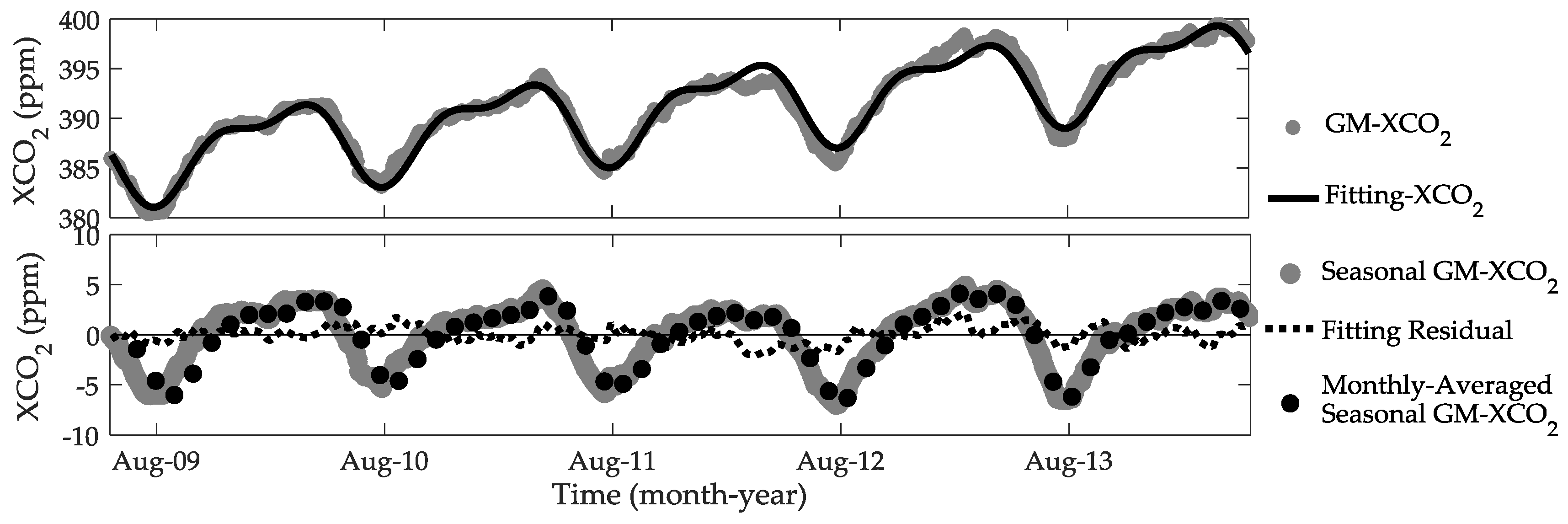
2.2. Calculation of Seasonal Cycle Amplitude of XCO2
2.3. Correlating Analysis of Seasonal Variation between XCO2 and Biosphere Parameters
3. Results
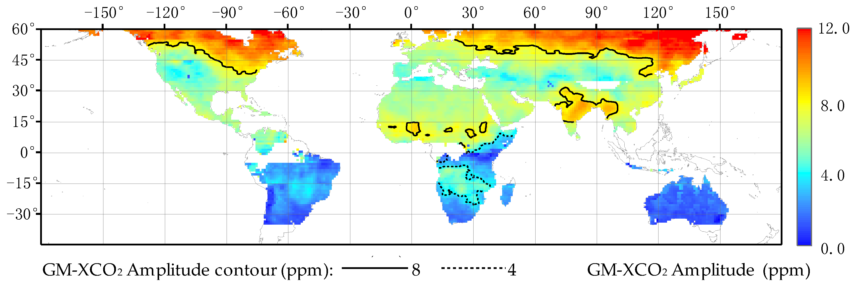
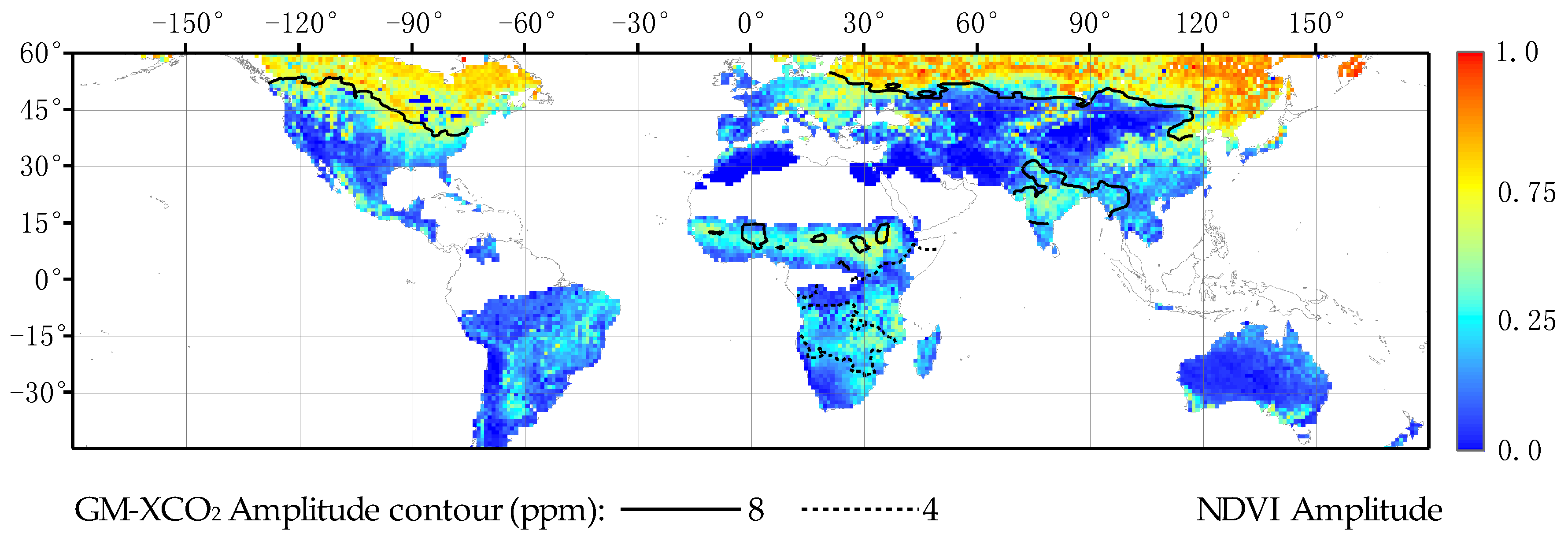
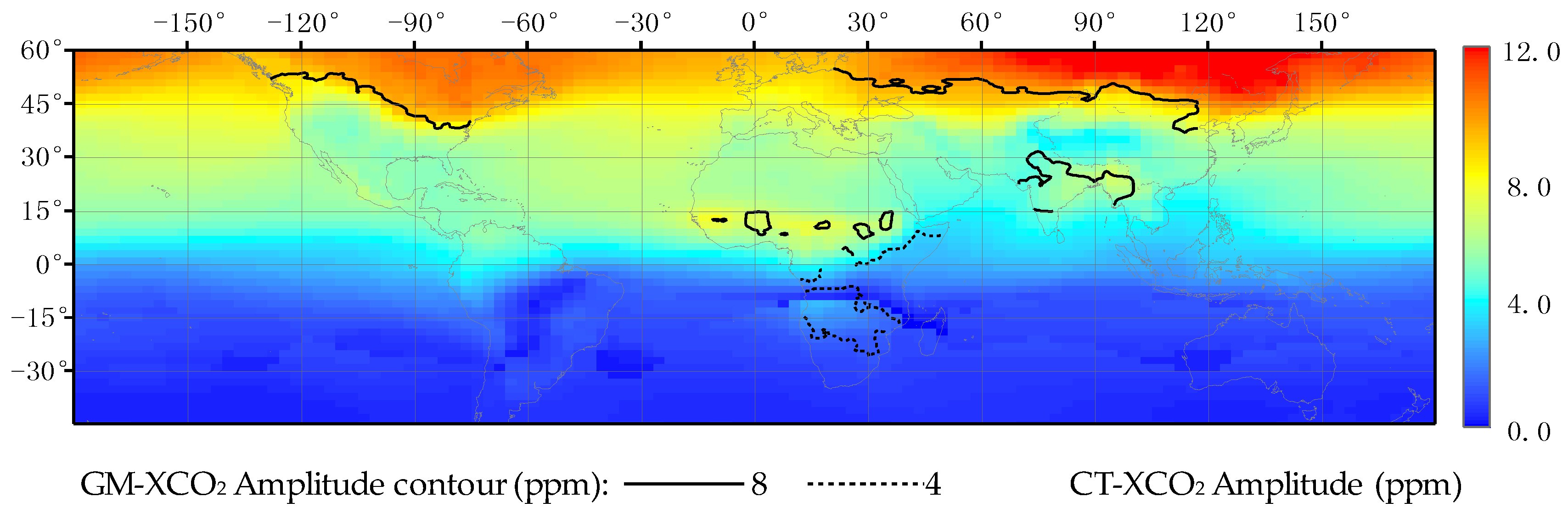
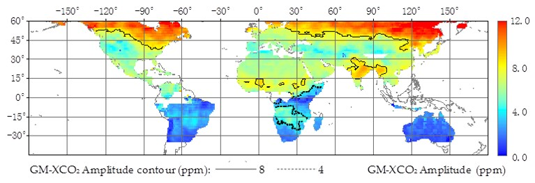
3.1. Spatial Pattern of Seasonal Cycle Amplitude of XCO2 and NDVI
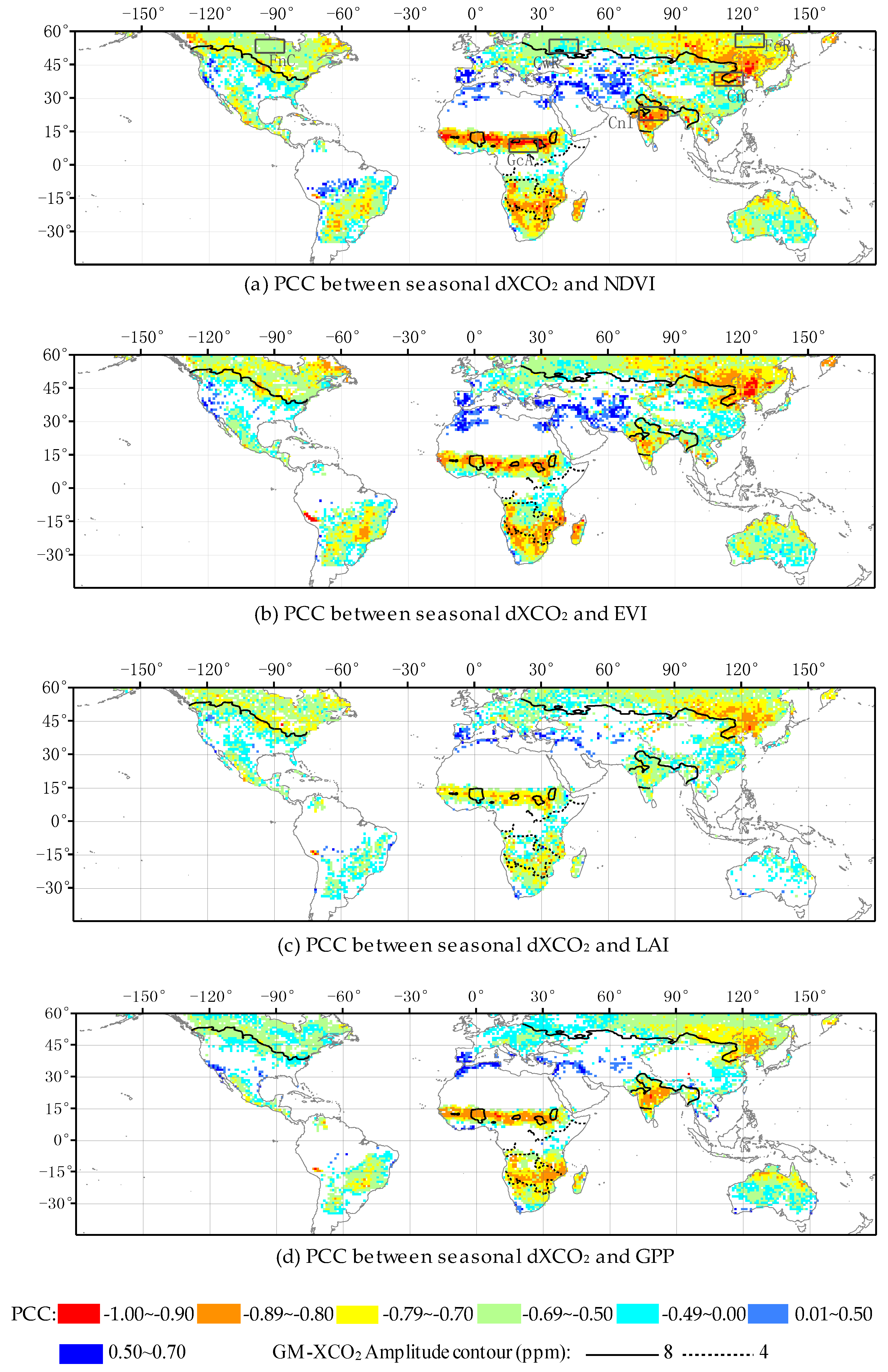
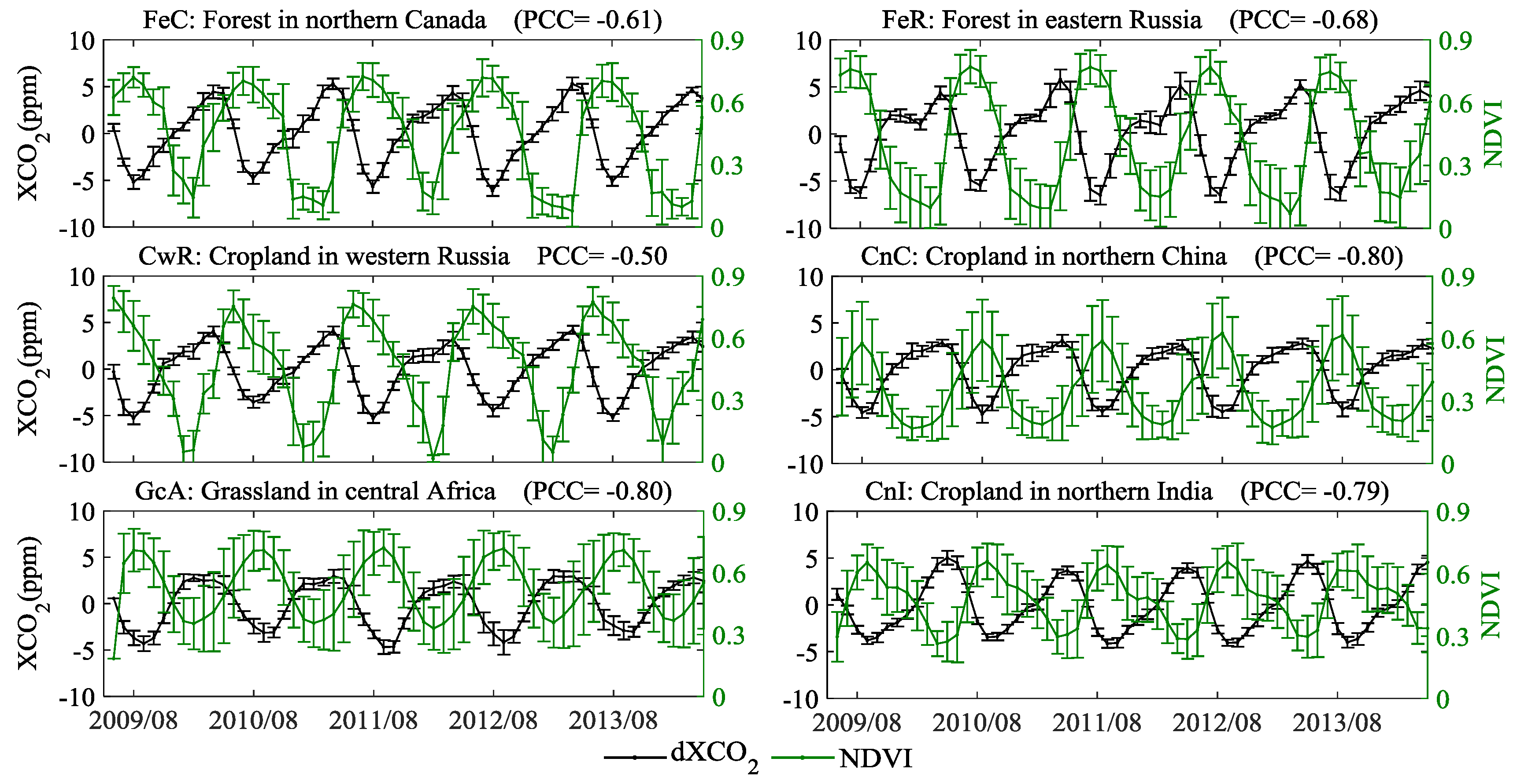
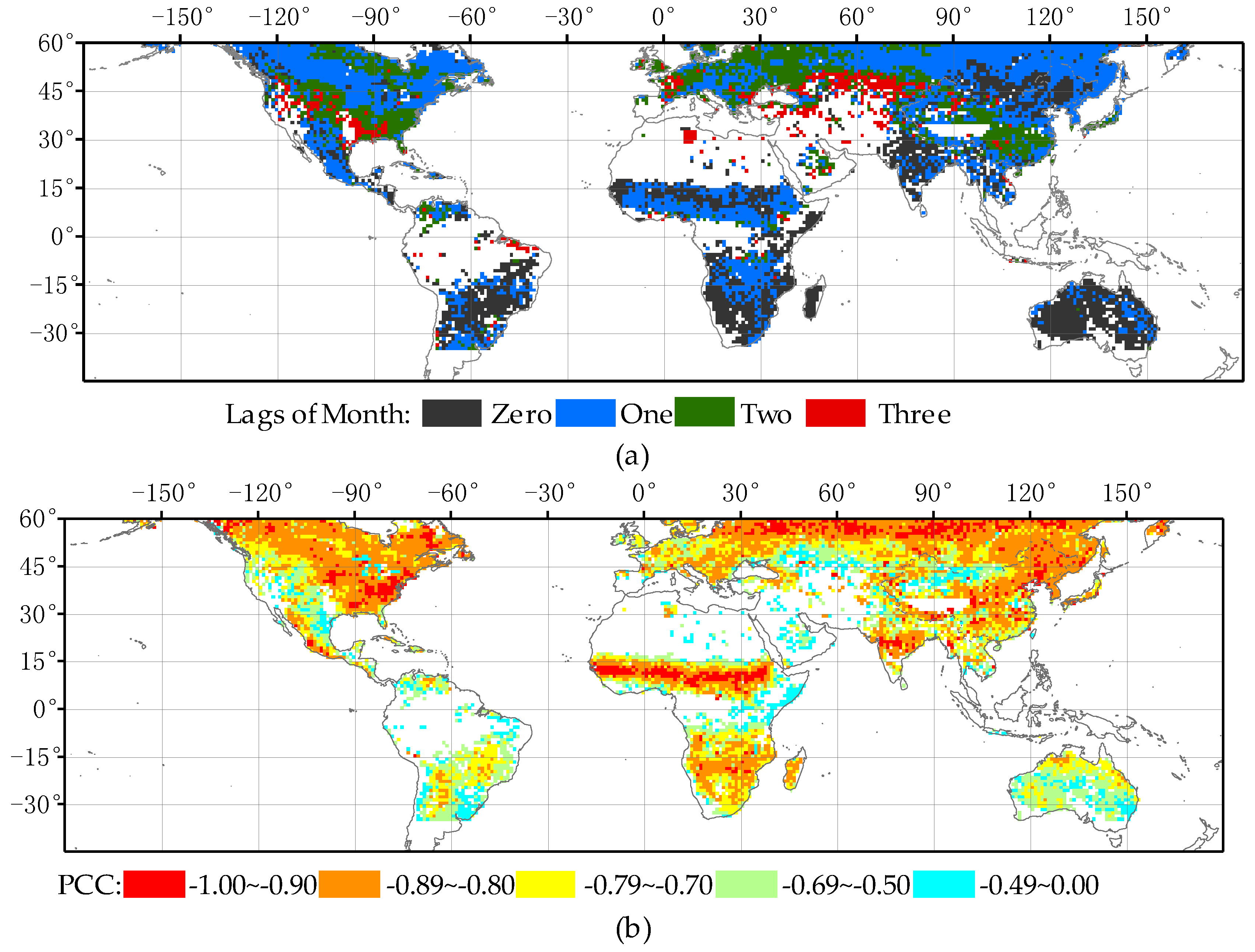
3.2. Correlation between XCO2 and Biosphere Parameters
3.3. Global Pattern of Phase Delay Effect of XCO2 to NDVI
4. Discussion
4.1. Uncertainty of XCO2 Global Land Mapping Dataset
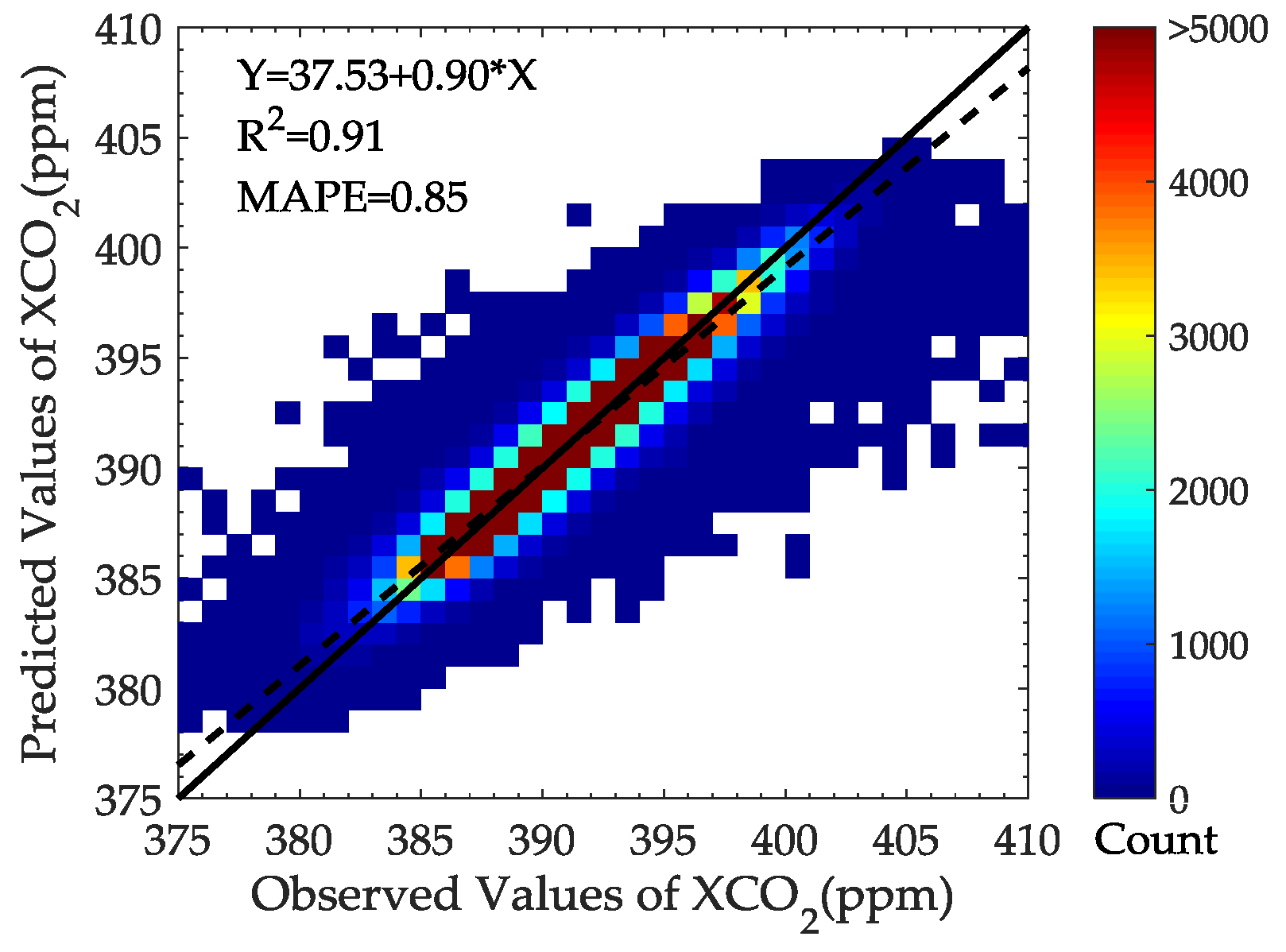
4.1.1. Evaluation Using Cross-Validation
4.1.2. Verification with TCCON
4.1.3. Comparison of Seasonal Cycle between GM-XCO2 and Model Simulations
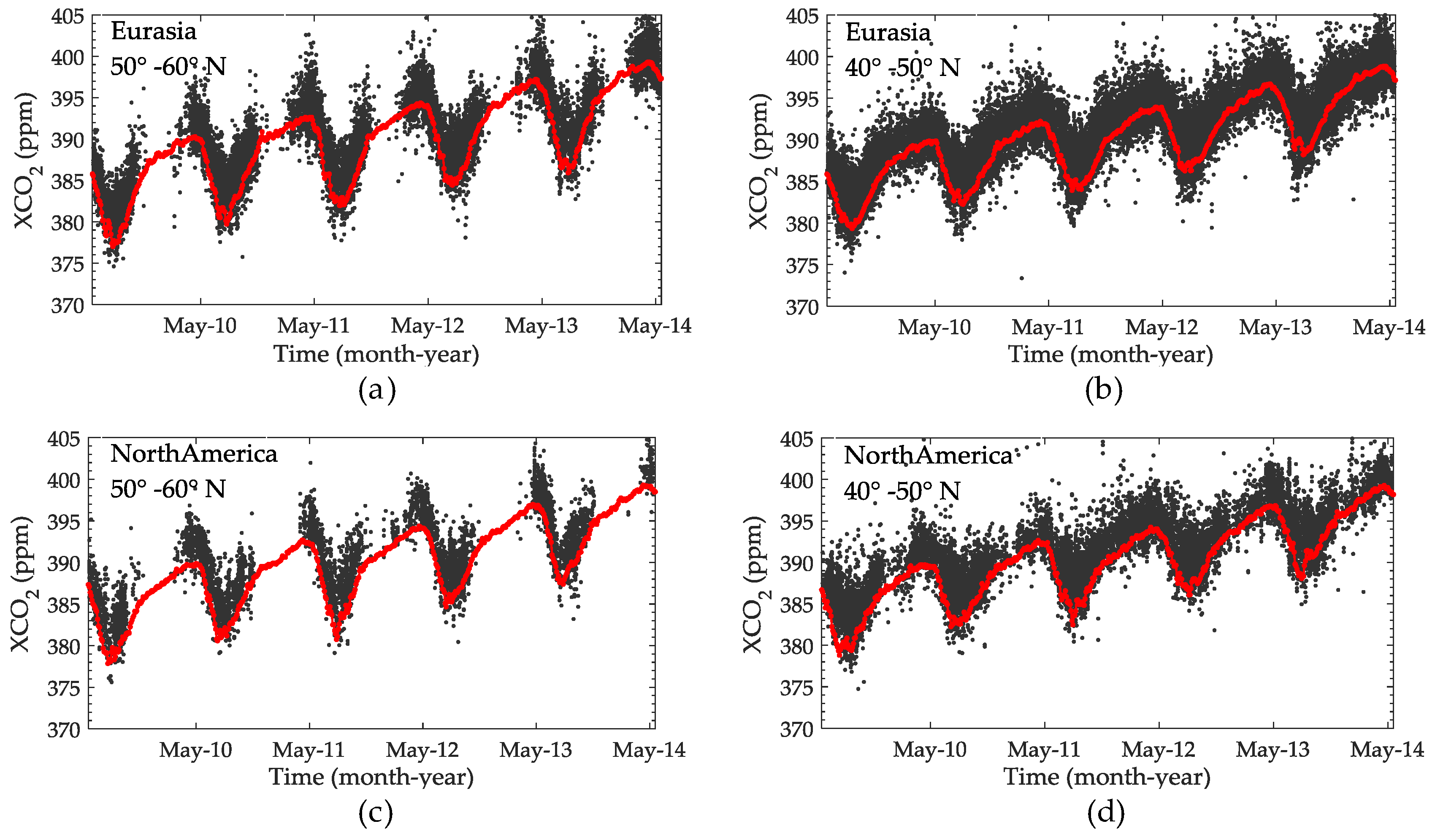
4.2. The Possible Impact of Retrieval Density in High Latitude Regions
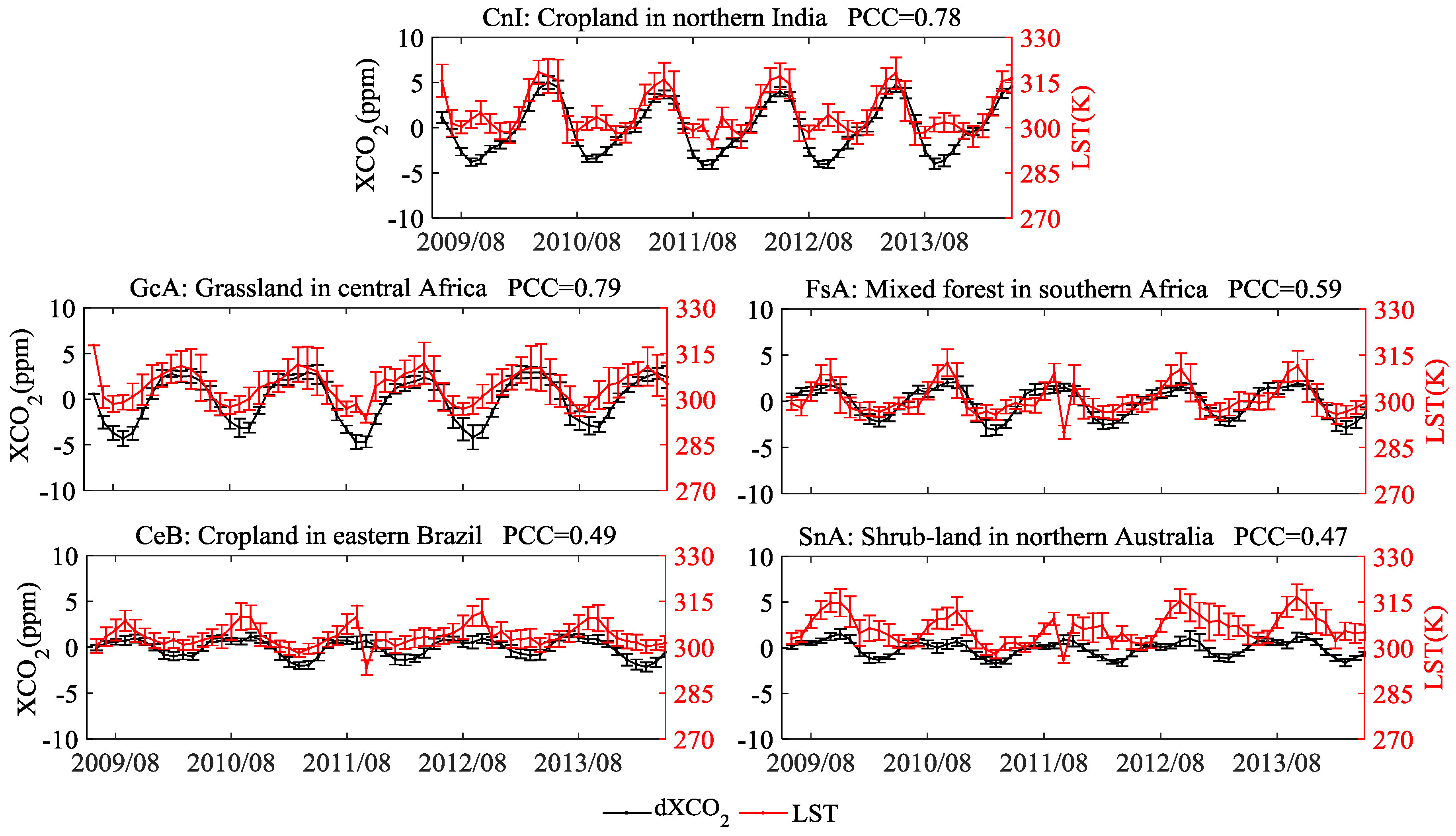
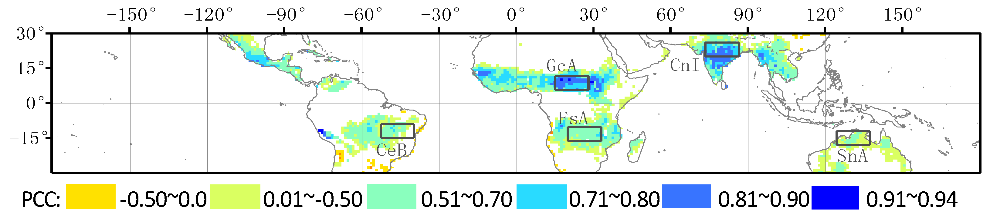
4.3. Possible Impact of LST on Seasonal Variation of XCO2 on Tropical Land
5. Conclusions
Supplementary Materials
Acknowledgments
Author Contributions
Conflicts of Interest
References
- Pan, Y.; Birdsey, R.A.; Fang, J.; Houghton, R.; Kauppi, P.E.; Kurz, W.A.; Phillips, O.L.; Shvidenko, A.; Lewis, S.L.; Canadell, J.G.; et al. A large and persistent carbon sink in the world’s forests. Science 2011, 333, 988–993. [Google Scholar] [CrossRef] [PubMed]
- Quéré, C.L.; Andres, R.J.; Boden, T.; Conway, T.; Houghton, R.; House, J.I.; Marland, G.; Peters, G.P.; Van der Werf, G.; Ahlström, A. The global carbon budget 1959–2011. Earth Syst. Sci. Data 2013, 5, 165–185. [Google Scholar] [CrossRef] [Green Version]
- Stocker, T.; Qin, D.; Plattner, G.; Tignor, M.; Allen, S.; Boschung, J.; Nauels, A.; Xia, Y.; Bex, B.; Midgley, B. Contribution of working group I to the fifth assessment report of the intergovernmental panel on climate change. In Climate Change 2013: The Physical Science Basis; Cambridge University Press: Cambridge, UK, 2013. [Google Scholar]
- Doney, S.C.; Lima, I.; Feely, R.A.; Glover, D.M.; Lindsay, K.; Mahowald, N.; Moore, J.K.; Wanninkhof, R. Mechanisms governing interannual variability in upper-ocean inorganic carbon system and air–sea CO2 fluxes: Physical climate and atmospheric dust. Deep Sea Res. Part II Top. Stud. Oceanogr. 2009, 56, 640–655. [Google Scholar] [CrossRef]
- Zeng, N.; Zhao, F.; Collatz, G.J.; Kalnay, E.; Salawitch, R.J.; West, T.O.; Guanter, L. Agricultural green revolution as a driver of increasing atmospheric CO2 seasonal amplitude. Nature 2014, 515, 394–397. [Google Scholar] [CrossRef] [PubMed]
- Keeling, R.F.; Piper, S.C.; Heimann, M. Global and hemispheric CO2 sinks deduced from changes in atmospheric concentration. Nature 1996, 381, 218–221. [Google Scholar] [CrossRef]
- Buermann, W.; Lintner, B.R.; Koven, C.D.; Angert, A.; Pinzon, J.E.; Tucker, C.J.; Fung, I.Y. The changing carbon cycle at Mauna Loa Observatory. Proc. Natl. Acad. Sci. USA 2007, 104, 4249–4254. [Google Scholar] [CrossRef] [PubMed]
- Forkel, M.; Carvalhais, N.; Rodenbeck, C.; Keeling, R.; Heimann, M.; Thonicke, K.; Zaehle, S.; Reichstein, M. Enhanced seasonal CO2 exchange caused by amplified plant productivity in northern ecosystems. Science 2016, 351, 696–699. [Google Scholar] [CrossRef] [PubMed]
- Graven, H.D.; Keeling, R.F.; Piper, S.C.; Patra, P.K.; Stephens, B.B.; Wofsy, S.C.; Welp, L.R.; Sweeney, C.; Tans, P.P.; Kelley, J.J. Enhanced seasonal exchange of CO2 by northern ecosystems since 1960. Science 2013, 341, 1085–1089. [Google Scholar] [CrossRef] [PubMed]
- Randerson, J.T.; Thompson, M.V.; Conway, T.J.; Fung, I.Y.; Field, C.B. The contribution of terrestrial sources and sinks to trends in the seasonal cycle of atmospheric carbon dioxide. Glob. Biogeochem. Cycles 1997, 11, 535–560. [Google Scholar] [CrossRef]
- Schneising, O.; Reuter, M.; Buchwitz, M.; Heymann, J.; Bovensmann, H.; Burrows, J.P. Terrestrial carbon sink observed from space: Variation of growth rates and seasonal cycle amplitudes in response to interannual surface temperature variability. Atmos. Chem. Phys. 2014, 14, 133–141. [Google Scholar] [CrossRef]
- Welp, L.R.; Patra, P.K.; Rödenbeck, C.; Nemani, R.; Bi, J.; Piper, S.C.; Keeling, R.F. Increasing summer net CO2 uptake in high northern ecosystems inferred from atmospheric inversions and comparisons to remote-sensing NDVI. Atmos. Chem. Phys. 2016, 16, 9047–9066. [Google Scholar] [CrossRef] [Green Version]
- Wunch, D.; Wennberg, P.O.; Messerschmidt, J.; Parazoo, N.C.; Toon, G.C.; Deutscher, N.M.; Aleks, G.K.; Roehl, C.M.; Randerson, J.T.; Warneke, T.; et al. The covariation of northern hemisphere summertime CO2 with surface temperature in boreal regions. Atmos. Chem. Phys. 2013, 13, 9447–9459. [Google Scholar] [CrossRef]
- Lindqvist, H.; O’Dell, C.W.; Basu, S.; Boesch, H.; Chevallier, F.; Deutscher, N.; Feng, L.; Fisher, B.; Hase, F.; Inoue, M.; et al. Does gosat capture the true seasonal cycle of carbon dioxide? Atmos. Chem. Phys. 2015, 15, 13023–13040. [Google Scholar] [CrossRef]
- Kulawik, S.; Wunch, D.; O'Dell, C.; Frankenberg, C.; Reuter, M.; Oda, T.; Chevallier, F.; Sherlock, V.; Buchwitz, M.; Osterman, G.; et al. Consistent evaluation of ACOS-GOSAT, BESD-SCIAMACHY, CarbonTracker, and MACC through comparisons to TCCON. Atmos. Meas. Tech. 2016, 9, 683–709. [Google Scholar] [CrossRef]
- Aleks, G.K.; Wennberg, P.O.; Washenfelder, R.A.; Wunch, D.; Schneider, T.; Toon, G.C.; Andres, R.J.; Blavier, J.F.; Connor, B.; Davis, K.J.; et al. The imprint of surface fluxes and transport on variations in total column carbon dioxide. Biogeosciences 2012, 9, 875–891. [Google Scholar] [CrossRef] [Green Version]
- Ciais, P.; Dolman, A.J.; Bombelli, A.; Duren, R.; Peregon, A.; Rayner, P.J.; Miller, C.; Gobron, N.; Kinderman, G.; Marland, G.; et al. Current systematic carbon-cycle observations and the need for implementing a policy-relevant carbon observing system. Biogeosciences 2014, 11, 3547–3602. [Google Scholar] [CrossRef] [Green Version]
- Schimel, D.; Pavlick, R.; Fisher, J.B.; Asner, G.P.; Saatchi, S.; Townsend, P.; Miller, C.; Frankenberg, C.; Hibbard, K.; Cox, P. Observing terrestrial ecosystems and the carbon cycle from space. Glob. Chang. Biol. 2015, 21, 1762–1776. [Google Scholar] [CrossRef] [PubMed]
- Zeng, Z.; Lei, L.; Hou, S.; Ru, F.; Guan, X.; Zhang, B. A regional gap-filling method based on spatiotemporal variogram model of columns. IEEE Trans. Geosci. Remote Sens. 2014, 52, 3594–3603. [Google Scholar] [CrossRef]
- Zeng, Z.C.; Lei, L.; Strong, K.; Jones, D.B.A.; Guo, L.; Liu, M.; Deng, F.; Deutscher, N.M.; Dubey, M.K.; Griffith, D.W.T.; et al. Global land mapping of satellite-observed CO2 total columns using spatio-temporal geostatistics. Int. J. Digit. Earth 2017, 10. [Google Scholar] [CrossRef]
- Chen, B.; Xu, G.; Coops, N.C.; Ciais, P.; Innes, J.L.; Wang, G.; Myneni, R.B.; Wang, T.; Krzyzanowski, J.; Li, Q.; et al. Changes in vegetation photosynthetic activity trends across the Asia-Pacific region over the last three decades. Remote Sens. Environ. 2014, 144, 28–41. [Google Scholar] [CrossRef]
- Inoue, Y.; Peñuelas, J.; Miyata, A.; Mano, M. Normalized difference spectral indices for estimating photosynthetic efficiency and capacity at a canopy scale derived from hyperspectral and CO2 flux measurements in rice. Remote Sens. Environ. 2008, 112, 156–172. [Google Scholar] [CrossRef]
- Vetter, P.; Schmid, W.; Schwarze, R. Spatio-temporal statistical analysis of the carbon budget of the terrestrial ecosystem. Stat. Methods Appl. 2016, 25, 1–19. [Google Scholar] [CrossRef]
- Huang, N.; Gu, L.; Black, T.A.; Wang, L.; Niu, Z. Remote sensing-based estimation of annual soil respiration at two contrasting forest sites. J. Geophys. Res. Biogeosci. 2015, 120, 2306–2325. [Google Scholar] [CrossRef]
- ESA. Available online: http://www.esa-landcover-cci.org/ (accessed on 15 October 2016).
- O’Dell, C.W.; Connor, B.; Bösch, H.; O’Brien, D.; Frankenberg, C.; Castano, R.; Christi, M.; Eldering, D.; Fisher, B.; Gunson, M.; et al. The ACOS CO2 retrieval algorithm—Part 1: Description and validation against synthetic observations. Atmos. Meas. Tech. 2012, 5, 99–121. [Google Scholar] [CrossRef]
- Peters, W.; Jacobson, A.R.; Sweeney, C.; Andrews, A.E.; Conway, T.J.; Masarie, K.; Miller, J.B.; Bruhwiler, L.M.; Petron, G.; Hirsch, A.I.; et al. An atmospheric perspective on North American carbon dioxide exchange: CarbonTracker. Proc. Natl. Acad. Sci. USA 2007, 104, 18925–18930. [Google Scholar] [CrossRef] [PubMed]
- Huete, A.; Didan, K.; van Leeuwen, W.; Miura, T.; Glenn, E. MODIS vegetation indices. In Land Remote Sensing and Global Environmental Change; Springer: Berlin/Heidelberg, Germany, 2011; pp. 579–602. [Google Scholar]
- Heinsch, F.A.; Reeves, M.; Votava, P.; Kang, S.; Milesi, C.; Zhao, M.; Glassy, J.; Jolly, W.M.; Loehman, R.; Bowker, C.F. GPP and NPP (MOD17A2/A3) products NASA MODIS land algorithm. In MOD17 User’s Guide; MODIS Land Team: Washington, DC, USA, 2003; pp. 1–57. [Google Scholar]
- Yang, W.; Tan, B.; Huang, D.; Rautiainen, M.; Shabanov, N.V.; Wang, Y.; Privette, J.L.; Huemmrich, K.F.; Fensholt, R.; Sandholt, I. MODIS leaf area index products: From validation to algorithm improvement. IEEE Trans. Geosci. Remote Sens. 2006, 44, 1885–1898. [Google Scholar] [CrossRef]
- Wan, Z. Collection-5 MODIS Land Surface Temperature Products Users’ Guide; ICESS, University of California: Santa Barbara, CA, USA, 2007. [Google Scholar]
- National Aeronautics and Space Administration (NASA). Available online: http://CO2web.jpl.nasa.gov (accessed on 15 October 2016).
- Doughty, C.E.; Goulden, M.L. Are tropical forests near a high temperature threshold? J. Geophys. Res. Biogeosci. 2008, 113, 1–12. [Google Scholar] [CrossRef]
- Cox, P.M.; Pearson, D.; Booth, B.B.; Friedlingstein, P.; Huntingford, C.; Jones, C.D.; Luke, C.M. Sensitivity of tropical carbon to climate change constrained by carbon dioxide variability. Nature 2013, 494, 341–344. [Google Scholar] [CrossRef] [PubMed]
- Wunch, D.; Wennberg, P.O.; Toon, G.C.; Connor, B.J.; Fisher, B.; Osterman, G.B.; Frankenberg, C.; Mandrake, L.; O’Dell, C.; Ahonen, P.; et al. A method for evaluating bias in global measurements of CO2 total columns from space. Atmos. Chem. Phys. 2011, 11, 12317–12337. [Google Scholar] [CrossRef]
- Wunch, D.; Toon, G.C.; Blavier, J.F.; Washenfelder, R.A.; Notholt, J.; Connor, B.J.; Griffith, D.W.; Sherlock, V.; Wennberg, P.O. The total carbon column observing network. Philos. Trans. Ser. A Math. Phys. Eng. Sci. 2011, 369, 2087–2112. [Google Scholar] [CrossRef] [PubMed]
- Washenfelder, R.A.; Toon, G.C.; Blavier, J.F.; Yang, Z.; Allen, N.T.; Wennberg, P.O.; Vay, S.A.; Matross, D.M.; Daube, B.C. Carbon dioxide column abundances at the Wisconsin tall tower site. J. Geophys. Res. 2006, 111. [Google Scholar] [CrossRef]
- Wennberg, P.O.; Roehl, C.; Wunch, D.; Toon, G.C.; Blavier, J.F.; Washenfelder, R.; Aleks, G.K.; Allen, N.; Ayers, J. TCCON Data from Park Falls, Wisconsin, USA, Release GGG2014R0; Carbon Dioxide Information Analysis Center: Oak Ridge, TN, USA, 2014.
- Warneke, T.; Messerschmidt, J.; Notholt, J.; Weinzierl, C.; Deutscher, N.; Petri, C.; Grupe, P.; Vuillemin, C.; Truong, F.; Schmidt, M.; et al. TCCON Data from Orleans, France, Release GGG2014R0; Carbon Dioxide Information Analysis Center: Oak Ridge, TN, USA, 2014.
- Sussmann, R.; Rettinger, M. TCCON Data from Garmisch, Germany, Release GGG2014R0; Carbon Dioxide Information Analysis Center: Oak Ridge, TN, USA, 2014.
- Hase, F.; Blumenstock, T.; Dohe, S.; Gross, J.; Kiel, M. TCCON Data from Karlsruhe, Germany, Release GGG2014R1; Carbon Dioxide Information Analysis Center: Oak Ridge, TN, USA, 2014.
- Notholt, J.; Petri, C.; Warneke, T.; Deutscher, N.; Buschmann, M.; Weinzierl, C.; Macatangay, R.; Grupe, P. TCCON Data from Bremen, Germany, Release GGG2014R0; Carbon Dioxide Information Analysis Center: Oak Ridge, TN, USA, 2014.
- Messerschmidt, J.; Chen, H.; Deutscher, N.M.; Gerbig, C.; Grupe, P.; Katrynski, K.; Koch, F.T.; Lavrič, J.V.; Notholt, J.; Rödenbeck, C.; et al. Automated ground-based remote sensing measurements of greenhouse gases at the Białystok site in comparison with collocated in situ measurements and model data. Atmos. Chem. Phys. 2012, 12, 6741–6755. [Google Scholar] [CrossRef]
- Deutscher, N.; Notholt, J.; Messerschmidt, J.; Weinzierl, C.; Warneke, T.; Petri, C.; Grupe, P.; Katrynski, K. TCCON Data from Bialystok, Poland, Release GGG2014R1; Carbon Dioxide Information Analysis Center: Oak Ridge, TN, USA, 2014.
- Ohyama, H.; Morino, I.; Nagahama, T.; Machida, T.; Suto, H.; Oguma, H.; Sawa, Y.; Matsueda, H.; Sugimoto, N.; Nakane, H.; et al. Column-averaged volume mixing ratio of CO2 measured with ground-based fourier transform spectrometer at Tsukuba. J. Geophys. Res. 2009, 114. [Google Scholar] [CrossRef]
- Morino, I.; Matsuzaki, T.; Shishime, A. TCCON Data from Tsukuba, Ibaraki, Japan, 125hr, Release GGG2014R1; Carbon Dioxide Information Analysis Center: Oak Ridge, TN, USA, 2014.
- Wennberg, P.O.; Wunch, D.; Roehl, C.; Blavier, J.F.; Toon, G.C.; Allen, N.; Dowell, P.; Teske, K.; Martin, C.; Martin, J. TCCON Data from Lamont, Oklahoma, USA, Release GGG2014R0; Carbon Dioxide Information Analysis Center: Oak Ridge, TN, USA, 2014.
- Wennberg, P.O.; Roehl, C.; Blavier, J.F.; Wunch, D.; Landeros, J.; Allen, N. TCCON Data from Jet Propulsion Laboratory, Pasadena, California, USA, Release GGG2014R0; Carbon Dioxide Information Analysis Center: Oak Ridge, TN, USA, 2014.
- Kawakami, S.; Ohyama, H.; Arai, K.; Okumura, H.; Taura, C.; Fukamachi, T.; Sakashita, M. TCCON Data from Saga, Japan, Release GGG2014R0; Carbon Dioxide Information Analysis Center: Oak Ridge, TN, USA, 2014.
- Griffith, D.W.T.; Deutscher, N.; Velazco, V.A.; Wennberg, P.O.; Yavin, Y.; Aleks, G.K.; Washenfelder, R.; Toon, G.C.; Blavier, J.F.; Murphy, C.; et al. TCCON Data from Darwin, Australia, Release GGG2014R0; Carbon Dioxide Information Analysis Center: Oak Ridge, TN, USA, 2014.
- Griffith, D.W.T.; Velazco, V.A.; Deutscher, N.; Murphy, C.; Jones, N.; Wilson, S.; Macatangay, R.; Kettlewell, G.; Buchholz, R.R.; Riggenbach, M. TCCON Data from Wollongong, Australia, Release GGG2014R0; Carbon Dioxide Information Analysis Center: Oak Ridge, TN, USA, 2014.
- Connor, B.J.; Boesch, H.; Toon, G.; Sen, B.; Miller, C.; Crisp, D. Orbiting carbon observatory: Inverse method and prospective error analysis. J. Geophys. Res. Atmos. 2008, 113, 1–14. [Google Scholar] [CrossRef]
- Cogan, A.J.; Boesch, H.; Parker, R.J.; Feng, L.; Palmer, P.I.; Blavier, J.F.L.; Deutscher, N.M.; Macatangay, R.; Notholt, J.; Roehl, C.; et al. Atmospheric carbon dioxide retrieved from the greenhouse gases observing satellite (GOSAT): Comparison with ground-based TCCON observations and GEOS-Chem model calculations. J. Geophys. Res. Atmos. 2012, 117, 1–17. [Google Scholar] [CrossRef]
- Keeling, C.D.; Bacastow, R.B.; Bainbridge, A.E.; Ekdahl, C.A.; Guenther, P.R.; Waterman, L.S.; Chin, J.F.S. Atmospheric carbon dioxide variations at Mauna Loa Observatory, Hawaii. Tellus 1976, 28, 538–551. [Google Scholar]
- Thoning, K.W.; Tans, P.P.; Komhyr, W.D. Atmospheric carbon dioxide at Mauna Loa Observatory: 2. Analysis of the NOAA GMCC data, 1974–1985. J. Geophys. Res. Atmos. 1989, 94, 8549–8565. [Google Scholar] [CrossRef]
- Jiang, X.; Chahine, M.T.; Li, Q.; Liang, M.; Olsen, E.T.; Chen, L.L.; Wang, J.; Yung, Y.L. CO2 semiannual oscillation in the middle troposphere and at the surface. Glob. Biogeochem. Cycles 2012, 26. [Google Scholar] [CrossRef]
- Schneising, O.; Buchwitz, M.; Reuter, M.; Heymann, J.; Bovensmann, H.; Burrows, J.P. Long-term analysis of carbon dioxide and methane column-averaged mole fractions retrieved from SCIAMACHY. Atmos. Chem. Phys. 2011, 11, 2863–2880. [Google Scholar] [CrossRef] [Green Version]
- Aleks, G.K.; Wennberg, P.O.; Schneider, T. Sources of variations in total column carbon dioxide. Atmos. Chem. Phys. 2011, 11, 3581–3593. [Google Scholar] [CrossRef]
- Gitelson, A.A.; Peng, Y.; Arkebauer, T.J.; Schepers, J. Relationships between gross primary production, green LAI, and canopy chlorophyll content in maize: Implications for remote sensing of primary production. Remote Sens. Environ. 2014, 144, 65–72. [Google Scholar] [CrossRef]
- Lausch, A.; Pause, M.; Schmidt, A.; Salbach, C.; Gwillymmargianto, S.; Merbach, I. Temporal hyperspectral monitoring of chlorophyll, LAI, and water content of barley during a growing season. Can. J. Remote Sens. 2013, 39, 191–207. [Google Scholar] [CrossRef]
- Huete, A.; Didan, K.; Miura, T.; Rodriguez, E.P.; Gao, X.; Ferreira, L.G. Overview of the radiometric and biophysical performance of the MODIS vegetation indices. Remote Sens. Environ. 2002, 83, 195–213. [Google Scholar] [CrossRef]
- Olsen, S.C.; Randerson, J.T. Differences between surface and column atmospheric CO2 and implications for carbon cycle research. J. Geophys. Res. 2004, 109. [Google Scholar] [CrossRef]
- Rayner, P.J.; Law, R.M. A Comparison of Modelled Responses to Prescribed CO2 Sources. In CSIRO Division of Atmospheric Research Technical Paper; CSIRO: Canberra, Australia, 1995. [Google Scholar]
- Huang, J.; McElroy, M.B. Contributions of the hadley and ferrel circulations to the energetics of the atmosphere over the past 32 years. J. Clim. 2014, 27, 2656–2666. [Google Scholar] [CrossRef]
- Aleks, G.K.; Wennberg, P.O.; O’Dell, C.W.; Wunch, D. Towards constraints on fossil fuel emissions from total column carbon dioxide. Atmos. Chem. Phys. 2013, 13, 4349–4357. [Google Scholar] [CrossRef]
- Liu, M.; Lei, L.; Liu, D.; Zeng, Z.C. Geostatistical analysis of CH4 columns over monsoon Asia using five years of GOSAT observations. Remote Sens. 2016, 8. [Google Scholar] [CrossRef]
- Nguyen, H.; Osterman, G.; Wunch, D.; O’Dell, C.; Mandrake, L.; Wennberg, P.; Fisher, B.; Castano, R. A method for colocating satellite XCO2 data to ground-based data and its application to ACOS-GOSAT and TCCON. Atmos. Meas. Tech. 2014, 7, 2631–2644. [Google Scholar] [CrossRef]
- Chevallier, F. On the statistical optimality of CO2 atmospheric inversions assimilating CO2 column retrievals. Atmos. Chem. Phys. 2015, 15, 11133–11145. [Google Scholar] [CrossRef]
- Heymann, J.; Schneising, O.; Reuter, M.; Buchwitz, M.; Rozanov, V.V.; Velazco, V.A.; Bovensmann, H.; Burrows, J.P. SCIAMACHY WFM-DOAS XCO2: Comparison with CarbonTracker XCO2 focusing on aerosols and thin clouds. Atmos. Meas. Tech. 2012, 5, 2887–2931. [Google Scholar] [CrossRef]
- Chandra, N.; Lal, S.; Venkataramani, S.; Patra, P.K.; Sheel, V. Temporal variations of atmospheric CO2 and CO at Ahmedabad in western India. Atmos. Chem. Phys. 2016, 16, 6153–6173. [Google Scholar] [CrossRef]
- Hammerling, D.M.; Michalak, A.M.; O’Dell, C.; Kawa, S.R. Global CO2 distributions over land from the greenhouse gases observing satellite (GOSAT). Geophys. Res. Lett. 2012, 39, 1–6. [Google Scholar] [CrossRef]
- Raich, J.W.; Potter, C. Global patterns of carbon dioxide emission from soils. Glob. Biogeochem. Cycles 1995, 9, 23–36. [Google Scholar] [CrossRef]
- Raich, J.W.; Potter, C.; Bhagawati, D. Interannual variability in global soil respiration, 1980–94. Glob. Chang. Biol. 2002, 8, 800–812. [Google Scholar] [CrossRef]
- Huang, N.; Gu, L.; Niu, Z. Estimating soil respiration using spatial data products: A case study in a deciduous broadleaf forest in the Midwest USA. J. Geophys. Res. Atmos. 2014, 119, 6393–6408. [Google Scholar] [CrossRef]
- Sreenivas, G.; Mahesh, P.; Subin, J.; Kanchana, A.L.; Rao, P.V.N.; Dadhwal, V.K. Influence of meteorology and interrelationship with greenhouse gases (CO2 and CH4) at a suburban site of India. Atmos. Chem. Phys. 2016, 16, 3953–3967. [Google Scholar] [CrossRef]
- Oda, T.; Maksyutov, S. A very high-resolution (1 km×1 km) global fossil fuel CO2 emission inventory derived using a point source database and satellite observations of nighttime lights. Atmos. Chem. Phys. 2011, 11, 543–556. [Google Scholar] [CrossRef]
- Andres, R.J.; Gregg, J.S.; Losey, L.; Marland, G.; Boden, T.A. Monthly, global emissions of carbon dioxide from fossil fuel consumption. Tellus B 2011, 63, 309–327. [Google Scholar] [CrossRef]
- Frank, A.B.; Karn, J.F. Vegetation indices, CO2 flux, and biomass for northern plains grasslands. J. Range Manag. 2003, 56, 382–387. [Google Scholar] [CrossRef]
- Aalto, T.; Ciais, P.; Chevillard, A.; Moulin, C. Optimal determination of the parameters controlling biospheric CO2 fluxes over Europe using eddy covariance fluxes and satellite NDVI measurements. Tellus B 2004, 56, 93–104. [Google Scholar] [CrossRef]
- Liu, Y.; Yang, D.; Cai, Z. A retrieval algorithm for Tansat XCO2 observation: Retrieval experiments using GOSAT data. Chin. Sci. Bull. 2013, 58, 1520–1523. [Google Scholar] [CrossRef]


| Dataset | Resolution Spatial Temporal | Description | Reference | |
|---|---|---|---|---|
| Global mapping XCO2 (GM-XCO2) | 1 × 1 degree | 3 day | Global land mapping of XCO2 by spatio-temporal geostatistics approach using GOSAT XCO2 (v 3.5) retrievals from ACOS project team. | Zeng et al. [20]; O’Dell et al. [26] |
| Simulated XCO2 (CT-XCO2) | 2 × 3 degree | 3 day | Global simulations of XCO2 derived from multi-layer CO2 data simulated by CarbonTracker CT2015 | Peter et al. [27] |
| NDVI | 0.05 degree | monthly | Normalized Difference Vegetation Index (NDVI) from MOD09 reflectance product (MYD13C2) | Huete et al. [28] |
| EVI | 0.05 degree | monthly | Enhanced Vegetation Index (EVI) from MOD09 reflectance product (MYD13C2) | Huete et al. [28] |
| GPP | 1 km | monthly | Gross Primary Productivity (GPP) from MODIS data product (MOD17A2) | Heinsch et al. [29] |
| LAI | 1 km | 8 days | Leaf Area Index (LAI) from MODIS data product (MCD15A2) | Yang et al. [30] |
| LST | 0.05 degree | monthly | Land Surface Temperature (LST) from MODIS data product (MOD11C3) | Wan et al. [31] |
| Regions | Long Name | Latitude | Longitude | Description | PCC with NDVI | PCC with LST |
|---|---|---|---|---|---|---|
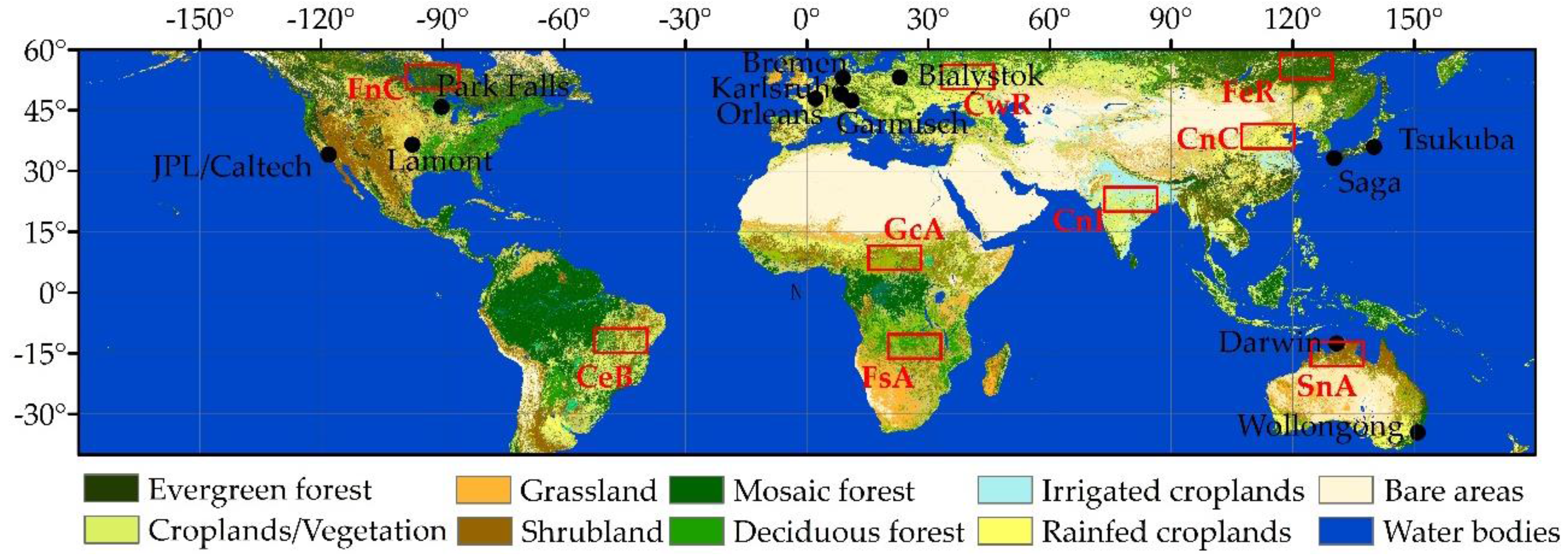
| FnC | Forest in Northern Canada | 50°–57°N | 86°–99°W | F: 63% | −0.61 | - |
| FeR | Forest in Eastern Russia | 52°–59°N | 117°–130°E | F: 86% | −0.68 | - |
| CwR | Cropland in Western Russia | 50°–57°N | 33°–46°E | C: 70% | −0.50 | - |
| CnC | Cropland in Northern China | 35°–42°N | 107°–120°E | C: 58% G-S: 18% | −0.80 | - |
| CnI | Cropland in Northern India | 19°–26°N | 74°–87°E | C: 89% | −0.79 | 0.78 |
| GcA | Grassland in Central Africa | 5°–12°N | 15°–28°E | G:36% F: 30% | −0.80 | 0.79 |
| CeB | Cropland in Eastern Brazil | 8°–15°S | 40°–53°W | C: 43% F: 15% | - | 0.49 |
| FsA | Mixed forest in Southern Africa | 10°–17°S | 20°–33°E | F: 64% | - | 0.59 |
| SnA | Shrub-land in Northern Australia | 11°–18°S | 124°–137°E | G: 60% | - | 0.47 |
| Sites | Location (Latitude, Longitude) | Coincident Data Pairs | Averaged Biases (ppm) | Averaged Absolute Bias (ppm) | Standard Deviation (ppm) | GM-XCO2 SCA (ppm) | TCCON SCA (ppm) | SCA Difference (ppm) |
|---|---|---|---|---|---|---|---|---|
| Bialystok | (53.23, 23.02) | 231 | 0.33 | 1.10 | 2.03 | 7.38 | 8.38 | −1.00 |
| Bremen | (53.1, 8.85) | 119 | −0.35 | 1.23 | 2.67 | 6.67 | 7.35 | −0.68 |
| Karlsruhe | (49.1, 8.44) | 193 | −0.57 | 1.33 | 2.59 | 6.12 | 7.50 | −1.38 |
| Orleans | (47.97, 2.11) | 259 | 0.21 | 1.11 | 1.94 | 5.87 | 7.62 | −1.75 |
| Garmisch | (47.48, 11.06) | 322 | −0.49 | 1.21 | 2.09 | 5.99 | 6.99 | −1.00 |
| Park Falls | (45.94, −90.27) | 453 | −0.24 | 1.02 | 1.62 | 9.25 | 9.2 | 0.05 |
| Lamont | (36.6, −97.49) | 513 | 0.25 | 0.95 | 1.40 | 5.18 | 5.8 | −0.62 |
| Tsukuba | (36.05, 140.12) | 246 | −1.72 | 1.94 | 2.70 | 7.38 | 6.38 | 1.00 |
| JPL/Caltech | (34.2, −118.18) | 195 | 0.10 | 1.29 | 2.45 | 5.32 | 6.07 | −0.75 |
| Saga | (33.24, 130.29) | 208 | 1.08 | 1.37 | 1.39 | 6.94 | 6.65 | 0.29 |
| Darwin | (−12.43, 130.89) | 413 | −0.36 | 1.02 | 1.37 | 2.27 | 1.12 | 1.15 |
| Wollongong | (−34.41, 150.88) | 412 | −0.36 | 0.68 | 0.65 | 1.34 | 1.41 | −0.07 |
| Overall | 3564 | −0.18 | 1.19 | 1.91 | −0.40 |
© 2017 by the authors. Licensee MDPI, Basel, Switzerland. This article is an open access article distributed under the terms and conditions of the Creative Commons Attribution (CC BY) license ( http://creativecommons.org/licenses/by/4.0/).
Share and Cite
He, Z.; Zeng, Z.-C.; Lei, L.; Bie, N.; Yang, S. A Data-Driven Assessment of Biosphere-Atmosphere Interaction Impact on Seasonal Cycle Patterns of XCO2 Using GOSAT and MODIS Observations. Remote Sens. 2017, 9, 251. https://doi.org/10.3390/rs9030251
He Z, Zeng Z-C, Lei L, Bie N, Yang S. A Data-Driven Assessment of Biosphere-Atmosphere Interaction Impact on Seasonal Cycle Patterns of XCO2 Using GOSAT and MODIS Observations. Remote Sensing. 2017; 9(3):251. https://doi.org/10.3390/rs9030251
Chicago/Turabian StyleHe, Zhonghua, Zhao-Cheng Zeng, Liping Lei, Nian Bie, and Shaoyuan Yang. 2017. "A Data-Driven Assessment of Biosphere-Atmosphere Interaction Impact on Seasonal Cycle Patterns of XCO2 Using GOSAT and MODIS Observations" Remote Sensing 9, no. 3: 251. https://doi.org/10.3390/rs9030251