Geostatistical Integration of Coarse Resolution Satellite Precipitation Products and Rain Gauge Data to Map Precipitation at Fine Spatial Resolutions

Abstract

This paper investigates the benefits of integrating coarse resolution satellite-derived precipitation estimates with quasi-point rain gauge data for generating a fine spatial resolution precipitation map product. To integrate the two precipitation data sources, a geostatistical downscaling and integration approach is presented that can account for the differences in spatial resolution between data from different supports and adjusts inherent errors in the coarse resolution precipitation estimates. First, coarse resolution precipitation estimates are downscaled at a fine spatial resolution via area-to-point kriging to allow direct comparison with rain gauge data. Second, the downscaled precipitation estimates are integrated with the rain gauge data by multivariate kriging. In particular, errors in the coarse resolution precipitation estimates are adjusted against rain gauge data during this second stage. In this study, simple kriging with local means (SKLM) and kriging with an external drift (KED) are used as multivariate kriging algorithms. For comparative purposes, conditional merging (CM), a frequently-applied method for integrating rain gauge data and radar precipitation, is also employed. From a case study with Tropical Rainfall Measuring Mission (TRMM) 3B43 monthly precipitation products acquired in South Korea from May–October in 2013, we found that the incorporation of TRMM data with rain gauge data did not improve prediction performance when the number of rain gauge data was relatively large. However, the benefit of integrating TRMM and rain gauge data was most striking, regardless of multivariate kriging algorithms, when a small number of rain gauge data was used. These results indicate that the coarse resolution satellite-derived precipitation product would be a useful source for mapping precipitation at a fine spatial resolution if the geostatistical integration approach is applied to areas with sparse rain gauges.

1. Introduction

Knowledge of the spatio-temporal variations in the distribution of precipitation is of critical importance to hydrological/hydrometeorological modeling. As the quality of hydrological and hydrometeorological model outputs depends greatly on the quality of the input precipitation estimates, realistic spatio-temporal distributions of precipitation are required for reliable modeling [1,2].

Two data sources are routinely used to obtain reliable estimates of precipitation. The first source comprises the point measurements acquired from rain gauges. The spatio-temporal estimates of precipitation are routinely obtained by applying various interpolation algorithms to the rain gauge data. It is not always possible, however, to generate reliable precipitation estimates from rain gauge data alone, as the quality of the resulting estimates depends on the number and spatial configuration of those data [3,4].

The second sources comprise radar or satellite observations. Weather radar, which measures the reflectivity of water droplets at a certain height [5,6], can provide fine resolution estimates of precipitation. However, such precipitation estimates suffer from various types of errors [7,8], so a proper correction of the radar estimates should be considered for many hydrological applications. In addition, weather radar networks are available only for restricted regions. Another source of quantitative precipitation data involves satellite-based estimates. Indeed, many missions producing satellite-derived precipitation estimates have been operating since the 1990s, such as the Tropical Rainfall Measuring Mission (TRMM) Multisatellite Precipitation Analysis (TMPA), the Global Precipitation Mapping (GPM) and the Global Change Observation Mission-Water (GCOM-W) [9,10,11]. These satellite precipitation products can provide periodic and regional information about the distribution of precipitation and its variations. Despite their advantages compared with rain gauge data, satellite precipitation products also have some limitations. First, their spatial resolution is too coarse to analyze precipitation distributions at a local scale. The spatial resolution of most satellite products ranges from 10 km–25 km, which is not adequate for local analysis. Thus, spatial downscaling to increase spatial resolution [12] is essential when using coarse spatial resolution satellite-derived precipitation data for local-scale analysis in areas where rain gauges are very sparse. Several statistical/geostatistical methods have been proposed for spatial downscaling, some of which integrate auxiliary environmental variables, such as elevation and vegetation index, at a fine spatial resolution via regression analysis and residual correction [4,13,14,15,16,17,18,19,20]. Promising downscaling results have been obtained by previous studies, but the predictive performance of any downscaling method is subject to the accuracy of input satellite precipitation product. A large number of rain gauges throughout the world is already used for precipitation retrieval from satellite data. For example, the TMPA 3B43 products have been rescaled by monthly rain gauge data from the Global Precipitation Climatological Project (GPCP) and the Climate Assessment and Monitoring System (CAMS) [21]. However, the accuracy of satellite-derived precipitation products might be unsatisfactory in some areas where accessibility to rain gauge data was restricted [22].

If properly integrated with satellite precipitation products, rain gauge data can be effectively used to map precipitation at a fine spatial resolution, since precipitation estimates from rain gauges and satellites have complementary characteristics in terms of data availability and accuracy. Precipitation data from rain gauges are usually regarded as true measurements, hence information provided by rain gauges could be used to adjust bias or errors in satellite precipitation products, thereby helping to improve the predictive performance of fine resolution mapping of precipitation.

Despite the potential of the integration of rain gauge data with satellite precipitation products, some challenging issues still need to be addressed. The major issue is the difference in scale between rain gauge data and satellite products. Rain gauge data can be regarded as point measurements, whereas satellite precipitation product can be considered as areal or aggregated measurements at a certain coarse spatial resolution. Thus, differences in scale or mismatching should be considered in an appropriate manner during the integration of data from different supports. A detailed discussion on the difficulty in comparing satellite-derived precipitation estimates with point rain gauges can be found in Porcù et al. [23]. In addition, an appropriate method should also be developed for the adjustment of satellite products using rain gauge data. As mentioned above, satellite precipitation products such as TMPA have been generated through a gauge adjustment step. However, the bias-corrected coarse resolution precipitation product might still have bias or errors at a finer resolution because rescaling to the monthly rain gauge data was implemented at the coarse resolution. Thus, local adjustment using rain gauge data is still required to generate improved precipitation estimates at the fine spatial resolution. To integrate rain gauges and satellite precipitation products, many studies have developed advanced methods, such as double kernel smoothing [24], Bayesian combination [25], conditional merging (CM) [26], cokriging (CK) [27] and kriging with an external drift (KED) [28,29,30]. Hunink et al. [31] combined two different TRMM products with rain gauge data and satellite-derived environmental variables, such as NDVI and DEM. However, this approach requires sufficient rain gauges to establish quantitative relationships between input variables. Although bias correction or local adjustment has been applied by the above methods, very few studies have considered the difference in scale during integration.

Recently, Duan and Bastiaanssen [32] tried to downscale TRMM 3B43 products with fine resolution environmental variables, and the downscaled TRMM precipitation estimates were then integrated with rain gauge data. The errors at rain gauges were interpolated, then added to correct the downscaled TRMM precipitation estimates. However, there was no step to relate the downscaled TRMM precipitation estimates to the rain gauge data prior to interpolation of the errors. The local adjustment with rain gauges may facilitate correcting errors in the downscaled satellite-derived precipitation estimates. When integrating rain gauges and satellite-derived precipitation estimates, the predictive performance usually depends on many factors. Even though the difference in scale has been properly accounted for, the spatial configuration or density of rain gauges, as well as the quality of the coarse resolution satellite precipitation product might affect the predictive performance. In particular, the density of rain gauges greatly affects not only the spatial pattern of mapping results, but also the degree of local adjustment of the satellite precipitation product. Therefore, the impact of the density of rain gauges on predictive performance should also be quantitatively evaluated, in conjunction with the development of a proper integration method. However, very few studies have considered these two important aspects in the same body of work.

In this study, we investigate the benefits of integrating coarse resolution satellite precipitation products and rain gauge data for fine resolution mapping of precipitation, with emphasis on the development of a geostatistical downscaling-integration framework. A two-stage geostatistical approach is presented that considers the differences in spatial resolution between rain gauge and satellite precipitation products, as well as the errors in satellite precipitation products. In the first stage, the coarse resolution satellite precipitation data are downscaled at a fine spatial resolution using area-to-point (ATP) kriging [33] to allow direct comparison with rain gauge data. In the second stage, the downscaled precipitation estimates are integrated with rain gauge data using multivariate kriging. During this second stage, the errors in the satellite-derived precipitation estimates are adjusted based on the rain gauge data. Three geostatistical algorithms, i.e., simple kriging with local means (SKLM), KED and CM, are applied for integration at a fine spatial resolution. To analyze the impact of the rain gauge density on the predictive performance, scenarios with various rain gauge densities are tested by cross-validation. Our approach differs from previous studies in that the whole of the procedures for both downscaling and integration is fully based on geostatistics that can provide consistent and flexible ways for the change of support, the quantification of spatial correlation and data integration. The methodological developments and applications are demonstrated by an experiment on the integration of TRMM monthly precipitation estimates and rain gauge data acquired over South Korea.

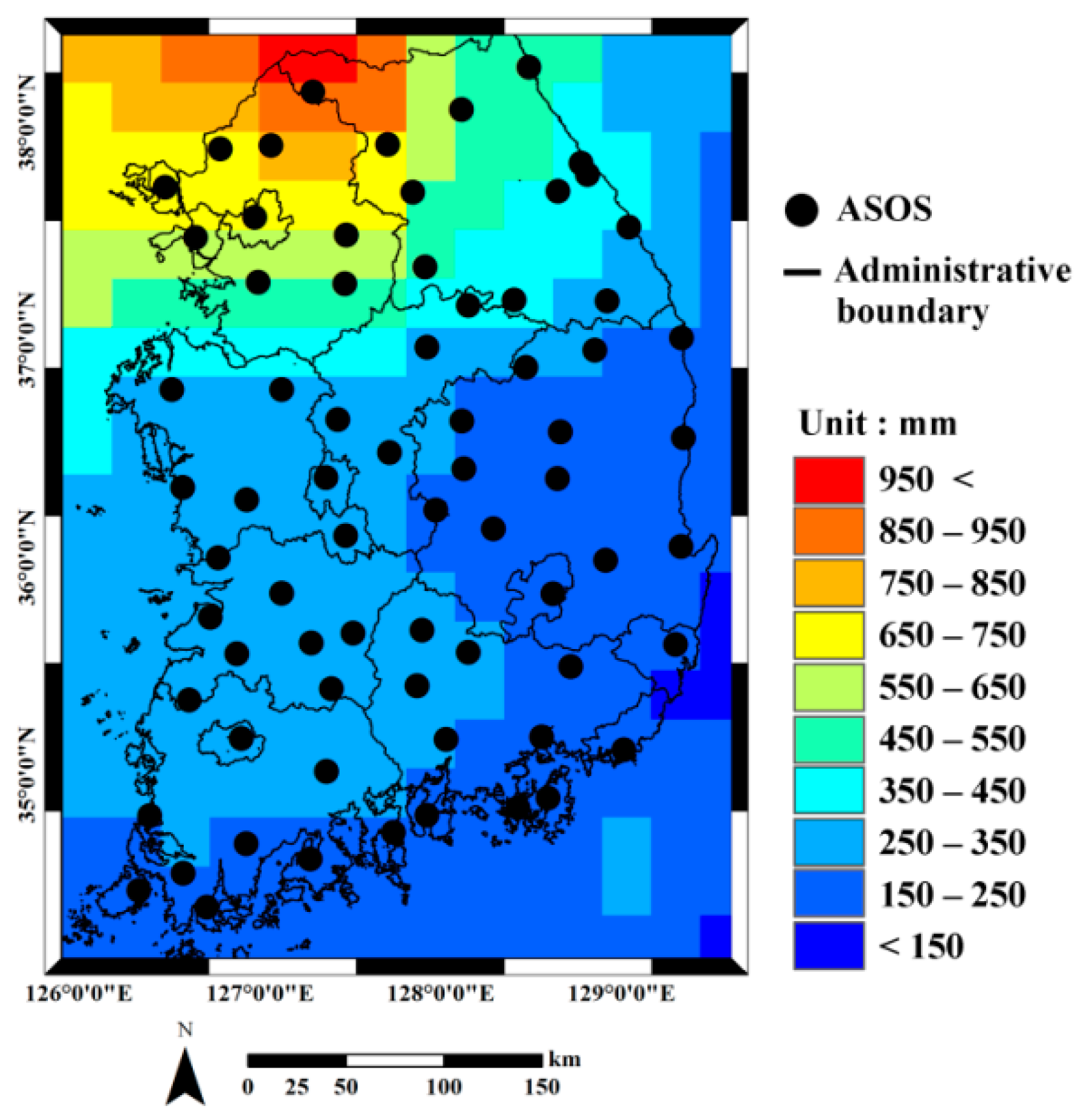
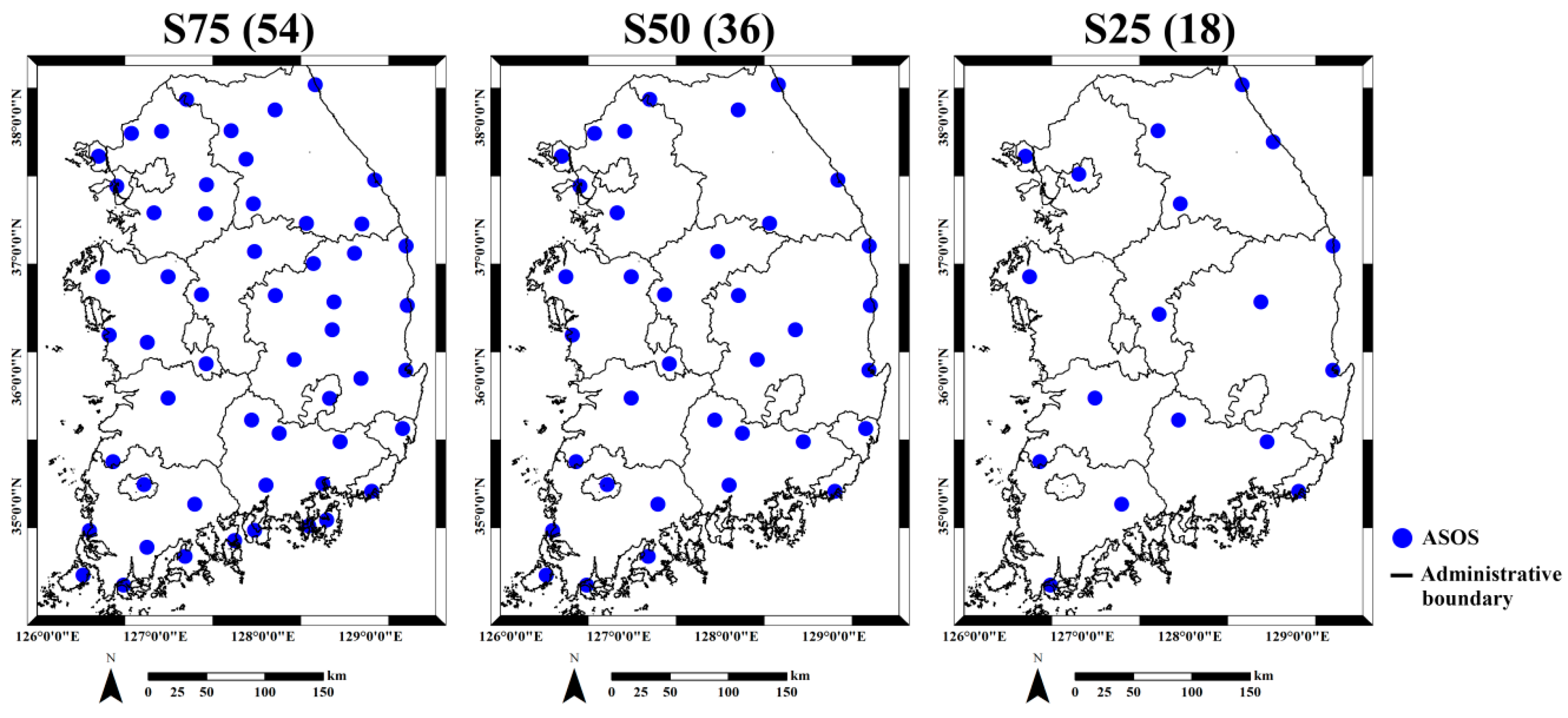
2. Study Area and Data

A downscaling and integration experiment is conducted using coarse resolution satellite precipitation products and rain gauge data acquired over South Korea. Six TRMM 3B43 products acquired from May–October in 2013 were used as the satellite-derived precipitation estimates. Using TRMM products from May–October, not all 12 months, is based on the precipitation characteristics in South Korea. Seasonally, 50%–60% of annual precipitation falls in summer, and the winter precipitation is less than 10% of the total annual precipitation [34]. As part of the summer East-Asian Monsoon system, a rainy season due to stationary front rain, locally known as the Changma in Korea, starts in late June and continues until late July, bringing frequent heavy rainfall [34,35]. Typhoons also have influences on the Korean peninsula from June–October [34]. By considering these precipitation characteristics in South Korea, TRMM products from May–October in 2013 were chosen for this experiment.

The original monthly TRMM data at a resolution of 0.25° were first geocoded using a transverse Mercator projection with a spatial resolution of 25 km. The monthly accumulated precipitation at a mm scale was finally prepared for integration with the rain gauge data. Monthly accumulated rainfall measurements obtained from 71 automated synoptic observing systems (ASOS) over South Korea were used for integrating and validating the prediction results (Figure 1). ASOS data are available mainly over land, so the integration and downscaling results were generated only over land. The target resolution for downscaling was set experimentally to 1 km.

3. Methodology

The geostatistical downscaling and integration approach employed in this study comprises two analytical steps (Figure 2): (1) downscaling of TRMM precipitation products using ATP kriging and (2) integration of rain gauge data with the downscaled TRMM precipitation products using multivariate kriging. A detailed description of each step is given in the following.

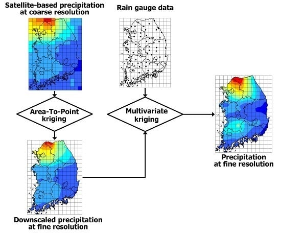
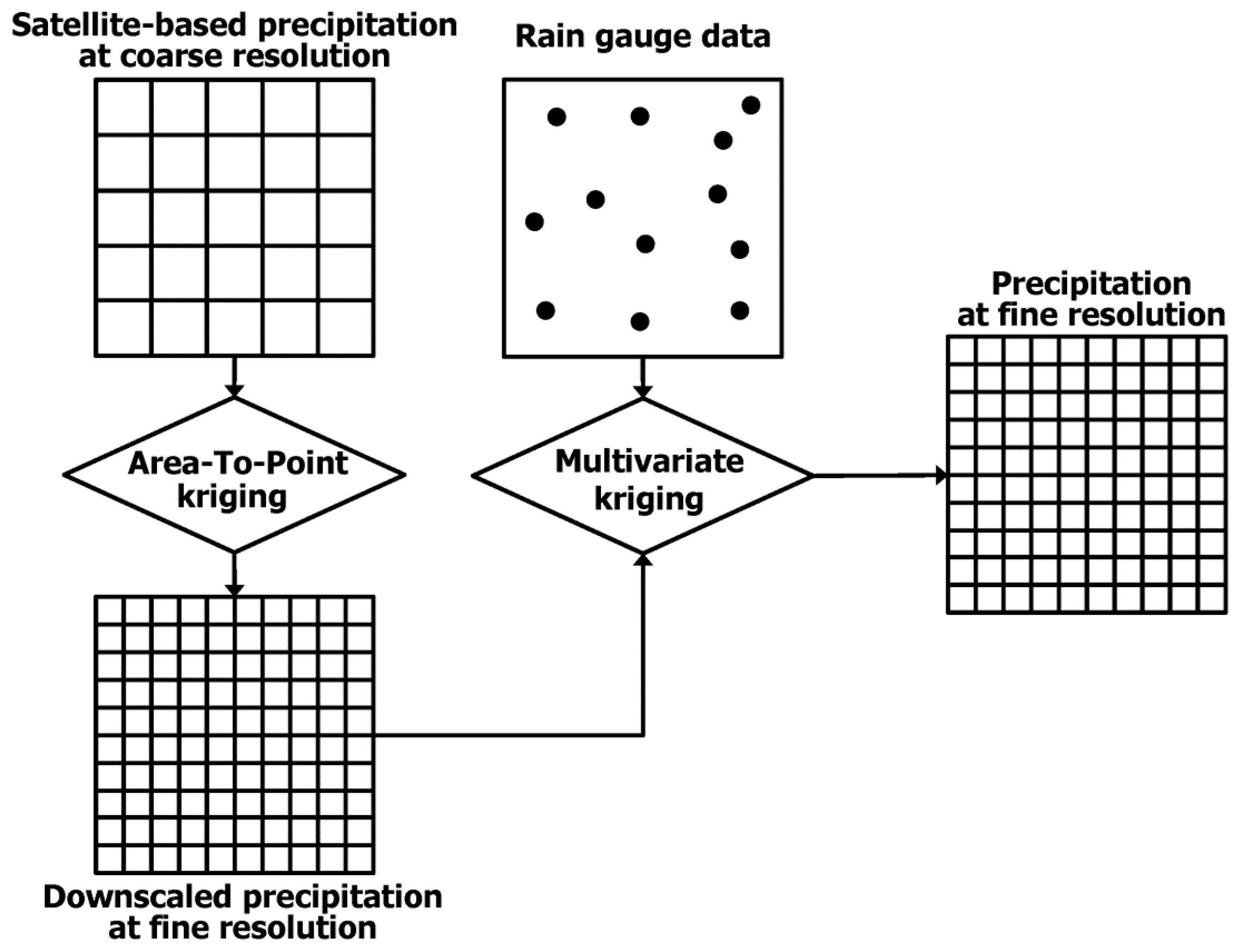
3.1. Geostatistical Downscaling

In the first processing step, ATP kriging is applied to obtain downscaled TRMM precipitation estimates at a 1-km resolution. The aim of this downscaling step is to compare the TRMM precipitation estimates with rain gauge data so as to facilitate both data integration and adjustment of errors in the TRMM data at a fine spatial resolution.

ATP kriging predicts target attribute values at a fine resolution (e.g., 1-km resolution in this study) by a linear combination of weighted neighboring attribute values at a coarse resolution [33,36,37]. If the TRMM precipitation product in the study area comprises N coarse pixels {$z(v_{\beta });\beta =1,\cdots ,N$} at the location $v_{\beta }$, then ATP ordinary kriging estimates are defined as:

$$z_{\mathrm{ATP}}^{\ast }(\mathbf{u})={\displaystyle \sum _{k=1}^K{\lambda }_k(\mathbf{u})z(v_k)}$$

(1)

where ${\lambda }_k(\mathbf{u})$ is an ordinary ATP kriging weight assigned to the K neighboring coarse pixels at a prediction location (u).

The ordinary ATP kriging weights are computed by solving the following ordinary block kriging system:

$$\begin{array}{l}{\displaystyle \sum _{k^{\prime }=1}^K{\lambda }_{k^{\prime }}(\mathbf{u})\overline{C}(v_k,v_{k^{\prime }})}+\mu (\mathbf{u})=\overline{C}(v_k,\mathbf{u}),k=1,\cdots ,K\\ {\displaystyle \sum _{k^{\prime }=1}^K{\lambda }_{k^{\prime }}(\mathbf{u})=1}\end{array}$$

(2)

where $\mu (\mathbf{u})$ is the Lagrange multiplier for the unit-sum constraint on the weights. $\overline{C}(v_i,v_j)$ and $\overline{C}(v_i,\mathbf{u})$ denote the block-to-block covariances and block-to-point covariances, respectively. The block-to-block covariances are numerically approximated based on the average of the covariances between any two points discretizing the coarse pixels $v_k$ and $v_{k^{\prime }}$. Similarly, the block-to-point covariances are computed by averaging the covariances between the prediction location u and a set of points discretizing the coarse pixel $v_k$ [33,37].

The computation of those two covariances requires the point-support covariance or equivalently the variogram. Spatial variability may change according to scale or support, so the variogram model inferred from coarse pixels cannot be used directly as the point-support variogram. In addition, the variogram model of rain gauge data cannot be used as the point-support variogram for the TRMM precipitation product because the latter data include errors and they may have different spatial variability. Thus, it is necessary to infer the point-support variogram from the available coarse pixels. In this study, the point-support variogram model is inferred using variogram deconvolution, which is an iterative procedure that aims to find the optimal point-support variogram model where the regularized model is very close to the variogram model of the coarse pixels [37]. More specifically, after defining an initial point-support variogram model, the theoretically regularized model is computed and compared with the variogram model inferred from the TRMM precipitation product. Based on the deviation between the two models, the parameters of the point-support model are adjusted, and the rescaled model is used for the next iteration. This procedure is repeated until the optimal model is finally found under predefined stop criteria [37].

After inferring the point-support variogram model by variogram deconvolution, ATP kriging estimates are obtained at 1-km resolution using Equations (1) and (2). These downscaled TRMM precipitation estimates are used as inputs to multivariate kriging for integration. If the same K coarse pixels are used for estimation at the prediction locations as the set of points for discretizing coarse pixels, then the average of ATP kriging estimates in the original coarse pixel is the same as the original TRMM precipitation value, which is called the coherence or consistency property [33,36]. Conventional interpolation methods such as inverse distance weighting cannot always satisfy this property. Thus, ATP kriging estimates can be regarded as downscaled TRMM precipitation estimates that preserve the characteristics of the original TRMM precipitation product at the resolution of 25 km.

3.2. Geostatistical Integration

After the TRMM precipitation product has been downscale to 1 km, it can be compared directly with the rain gauge data. Thus, the next step is to integrate and adjust the downscaled product with rain gauge data. Three multivariate kriging algorithms are used for integration in this study, i.e., SKLM, KED and CM. In these algorithms, rain gauge and downscaled TRMM product are regarded as point hard and exhaustive soft data, respectively. CK has been widely used for integrating hard and soft data, but it is not considered in this study because it requires more variogram modeling effort.

3.2.1. Simple Kriging with Local Means

SKLM, which is also called regression kriging [38], replaces the constant global means in univariate simple kriging by varying local means [39]. The local means are estimated based on quantitative relationships between collocated hard and soft data [39].

Suppose there are two information sources for precipitation prediction, i.e., rain gauge data {$z({\mathbf{u}}_{\alpha });\alpha =1,\cdots ,n$} and the downscaled TRMM precipitation ($z_{\mathrm{ATP}}^{\ast }(\mathbf{u})$). The SKLM estimates are defined as:

$$z_{\mathrm{SKLM}}^{\ast }(\mathbf{u})=m(\mathbf{u})+{\displaystyle \sum _{\alpha =1}^{n(\mathbf{u})}{\lambda }_{\alpha }(\mathbf{u})[z({\mathbf{u}}_{\alpha })}-m({\mathbf{u}}_{\alpha })]$$

(3)

where $n(\mathbf{u})$ is the number of rain gauge data within a predefined search window. $m(\mathbf{u})$ and $m({\mathbf{u}}_{\alpha })$ are the local means at the prediction location u and sample location ${\mathbf{u}}_{\alpha }$, respectively.

The local means $m({\mathbf{u}}_{\alpha })$ at rain gauges are first estimated by linear regression between $z({\mathbf{u}}_{\alpha })$ and $z_{\mathrm{ATP}}^{\ast }({\mathbf{u}}_{\alpha })$, where the former is the dependent variable and the latter is the independent variable. Since downscaled TRMM precipitation data are available for the study area, the local means $m(\mathbf{u})$ in the study area are finally obtained using the regression relationship, i.e., the TRMM precipitation estimates adjusted with respect to the rain gauge data are used as varying local means.

The term [$z({\mathbf{u}}_{\alpha })-m({\mathbf{u}}_{\alpha })$] in Equation (3) can be regarded as residuals. Thus, the kriging weights assigned to the residuals at rain gauges are computed using the following simple kriging system:

$${\displaystyle \sum _{\beta =1}^{n(\mathbf{u})}{\lambda }_{\beta }(\mathbf{u})C_R({\mathbf{u}}_{\alpha }-{\mathbf{u}}_{\beta })}=C_R({\mathbf{u}}_{\alpha }-\mathbf{u}),\alpha =1,\cdots ,n(\mathbf{u})$$

(4)

where $C_R$ is the covariance of the residuals.

The final SKLM estimates are obtained from Equations (3) and (4) by adding local means to the residual estimates. From a data integration viewpoint, the errors in the TRMM precipitation estimates are adjusted by regression using rain gauge data, which are assumed to be precise. In addition, spatial auto-correlation information is used for spatial prediction of the residuals that cannot be accounted for by the TRMM precipitation estimates.

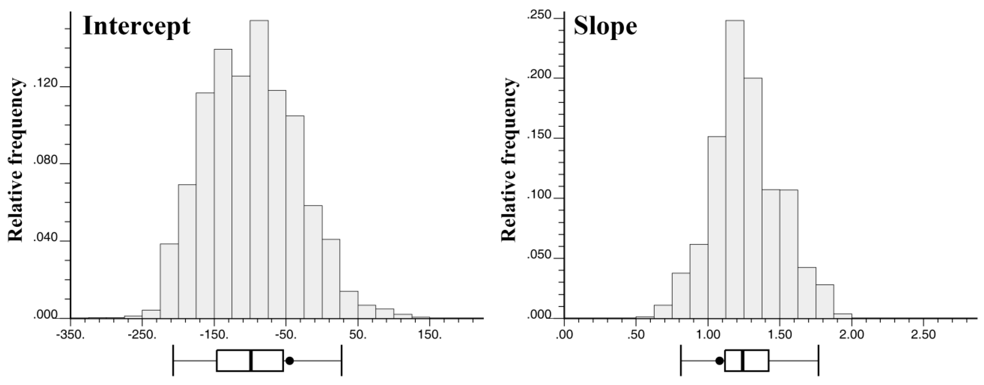
3.2.2. Kriging with an External Drift

KED is a multivariate kriging algorithm that can be applied when exhaustive soft data are available on a regular grid [39]. Similar to SKLM, KED also uses exhaustive downscaled TRMM precipitation estimates to derive varying local means, but KED differs from SKLM in that the soft data should have a linear relationship with the hard data, where the linear relationship is implicitly re-estimated by the kriging system. In other words, constant global regression coefficients are applied to the downscaled TRMM precipitation to derive the local means in SKLM, whereas the regression coefficients are locally re-estimated in KED. The KED estimates are computed as follows.

$$z_{\mathrm{KED}}^{\ast }(\mathbf{u})={\displaystyle \sum _{\alpha =1}^{n(\mathbf{u})}{\lambda }_{\alpha }(\mathbf{u})z({\mathbf{u}}_{\alpha })}$$

(5)

It should be noted that the regression coefficients and downscaled TRMM precipitation data are not included in Equation (5) because the locally re-estimated regression coefficients are generally used for interpretation purposes [3,39], rather than for the KED estimates.

The kriging weights are computed using the following KED kriging system:

$$\begin{array}{l}{\displaystyle \sum _{\beta =1}^{n(\mathbf{u})}{\lambda }_{\beta }(\mathbf{u})C_R({\mathbf{u}}_{\alpha }-{\mathbf{u}}_{\beta })}+{\mu }_0(\mathbf{u})+{\mu }_1(\mathbf{u})z_{\mathrm{ATP}}^{\ast }({\mathbf{u}}_{\alpha })=C_R({\mathbf{u}}_{\alpha }-\mathbf{u}),\alpha =1,\cdots ,n(\mathbf{u})\\ {\displaystyle \sum _{\beta =1}^{n(\mathbf{u})}{\lambda }_{\beta }(\mathbf{u})=1}\\ {\displaystyle \sum _{\beta =1}^{n(\mathbf{u})}{\lambda }_{\beta }(\mathbf{u})z_{\mathrm{ATP}}^{\ast }({\mathbf{u}}_{\alpha })}=z_{\mathrm{ATP}}^{\ast }(\mathbf{u})\end{array}$$

(6)

where ${\mu }_1(\mathbf{u})$ and ${\mu }_2(\mathbf{u})$ are two Lagrange multipliers for the constraints on the weights, and $C_R$ is the covariance of the residuals.

Unlike SKLM where the residuals are available at rain gauges, the residuals are not available in KED, so the residual variogram is not available. Several methods have been proposed for inferring the residual variogram. Since the trends or local means are already explained by exhaustive soft data, the residual variogram should be inferred from sample data pairs that are not affected or slightly affected by the trend [39] (p. 195). By following the practice of previous studies [40,41], the residual variogram inferred in SKLM was used for KED in the present study.

3.2.3. Conditional Merging

CM, which has been frequently employed to integrate rain gauge and radar data because of its computational efficiency, is a variant of kriging of errors [42]. CM combines the mean precipitation field estimated by kriging of rain gauge data and the spatial variability of soft data, such as radar or satellite precipitation product [26,42,43].

First, ordinary kriging (OK) using rain gauge data is employed to derive initial precipitation estimates. Next, the downscaled TRMM precipitation estimates only at rain gauges are interpolated over the study area. The differences between the interpolated and observed downscaled TRMM precipitation estimates over the study area are computed and regarded as errors, which are then added to the initial estimates obtained by OK using rain gauges. There are no differences at rain gauges, so the hard data values at rain gauges can be preserved (i.e., the exactitude property of kriging). The intrinsic assumption of CM is that exhaustive soft data can provide the overall spatial distributions of precipitation, although they may include local errors. In SKLM and KED, the errors in soft data are adjusted using rain gauge data, whereas CM uses soft data to estimate and adjust the errors associated with kriging of sparse rain gauges. Thus, CM estimates are affected by both the configuration of the rain gauge data and the quality of the downscaled TRMM precipitation estimates.

3.3. Performance Evaluation

This study was initiated to investigate whether merging rain gauge data and the satellite precipitation product could improve the predictive performance in fine resolution mapping of precipitation. For this purpose, different rain gauge density scenarios are considered in the performance evaluation. The impact of the rain gauge density scenarios on the predictive performance of different kriging algorithms is evaluated using leave-one-out cross-validation (LOO CV). Four sampling density scenarios were considered in this study: 100% (referred to as S100), 75% (S75), 50% (S50) and 25% (S25) of 71 rain gauges. If random sampling is applied to each density scenario, the predictive performance might be affected greatly by sampling fluctuations. Thus, to reduce the impact of the sampling fluctuations caused by random sampling, a systematic procedure to select representative rain gauges [30] is employed. The sum of the distances to the four nearest rain gauges is first computed. The rain gauges with the minimum distance (i.e., too close to neighbors) are then removed. However, when this principle is directly applied to rain gauges in the study area, as shown in Figure 1, most of the rain gauges near the coast are selected, and others on land are removed in S25. To avoid this problem, the selection procedure is serially repeated with respect to the remaining rain gauges. Therefore, the rain gauges with the maximum distance are retained, and the rain gauges in the low density scenario are always included in all of the other scenarios. The distributions of the rain gauges in each scenario are shown in Figure 3.

The error statistics are calculated based on LOO CV for each scenario. The relative mean bias (rME), root mean squared errors (RMSE) and relative RMSE (rRMSE) are computed as quantitative measures of errors. rME measures the relative degree of bias, whereas the latter two metrics measure the magnitude of errors. The amount of accumulated precipitation varies per month, so rRMSE is computed to compare the predictive performance for each month. To investigate the effects of integrating TRMM precipitation estimates, the relative improvement index (RI), which measures the improvement in RMSE compared with that in OK using only rain gauges, is also computed. Kriging is a generalized least square interpolator, so a smoothing effect is frequently observed in the predictions. To quantitatively measure the magnitude of the smoothing effect, the relative variance (rVar) is also computed. If any interpolator yields less smoothing effect, the value of rVar is close to 100%. If $z^{\ast }({\mathbf{u}}_{\alpha })$ and $z^{\ast }({\mathbf{u}}_{\alpha })$ are the predicted and true precipitation values at rain gauges, respectively, the equations of the measures above are as follows:

$$\mathrm{rME}(\%)=\frac{\frac{1}{n}{\displaystyle \sum _{\alpha =1}^n[z^{\ast }({\mathbf{u}}_{\alpha })-z({\mathbf{u}}_{\alpha })]}}{\overline{z}}\times 100$$

(7)

$$\mathrm{RMSE}=\sqrt{\frac{1}{n}{\displaystyle \sum _{\alpha =1}^n{[z^{\ast }({\mathbf{u}}_{\alpha })-z({\mathbf{u}}_{\alpha })]}^2}}$$

(8)

$$\mathrm{rRMSE}(\%)=\frac{\mathrm{RMSE}}{\overline{z}}\times 100$$

(9)

$${\mathrm{RI}}_i(\%)=\frac{{\mathrm{RMSE}}_{\mathrm{OK}}-{\mathrm{RMSE}}_i}{{\mathrm{RMSE}}_{\mathrm{OK}}}\times 100$$

(10)

$$\mathrm{rVar}(\%)=\frac{\mathrm{Var}[z^{\ast }({\mathbf{u}}_{\alpha })]}{\mathrm{Var}[z({\mathbf{u}}_{\alpha })]}\times 100$$

(11)

where n and $\overline{z}$ are the total number of rain gauges and the average of true precipitation values at rain gauges in each scenario, respectively. RMSE_i and RMSE_OK denote RMSE for the i-th interpolator and OK, respectively, and Var[·] is the variance of a certain variable.

4. Results

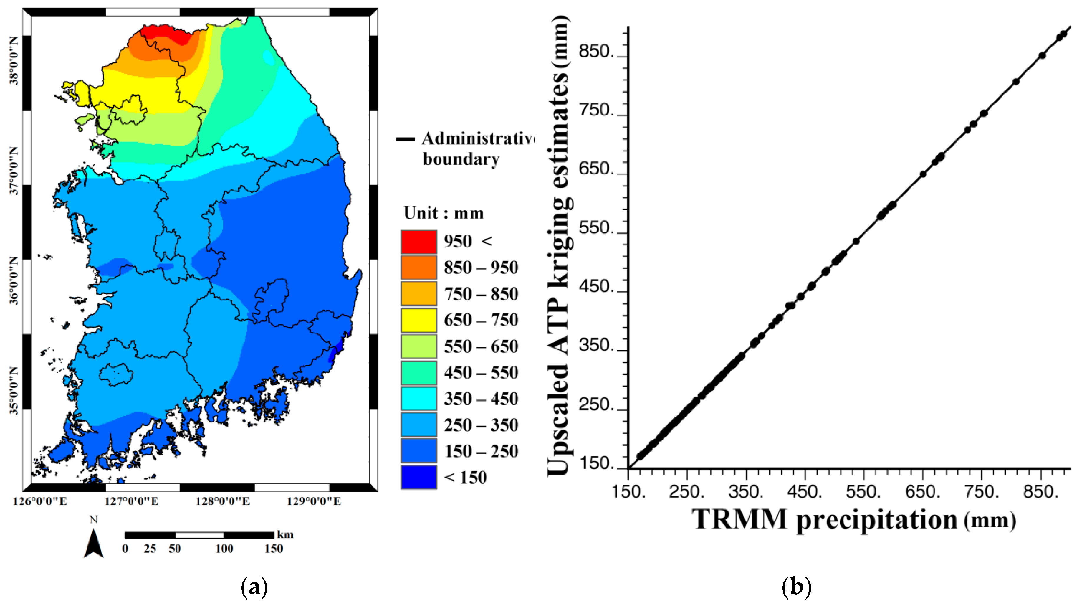
4.1. Downscaling of TRMM Precipitation Products

ATP kriging was implemented using FORTRAN and R programming. The neighboring 24 TRMM pixels were used for computing ATP kriging weights. The 1-km pixel, downscaled TRMM precipitation estimates for July, along with the scatter-plot illustrating the coherency property of the corresponding estimates are shown in Figure 4a,b, respectively. Note that some TRMM ocean pixels were excluded for upscaling because downscaling was performed only for land. The downscaled TRMM precipitation estimates at 1-km resolution generated by ATP kriging for all months preserved the overall patterns in the original TRMM precipitation products and reproduced the original TRMM precipitation values when upscaled to 25 km.

The downscaled TRMM precipitation estimates were compared directly with all of the rain gauge data, and the error statistics are presented in

Table 1. Summary of error statistics for the downscaled TRMM precipitation estimates. rME, relative mean bias; rRMSE, relative RMSE; rVar, relative variance.

Month	rME (%)	RMSE (mm)	rRMSE (%)	rVar (%)	Correlation
May	1.42	31.61	24.28	44.46	0.81
June	12.44	36.51	36.13	36.75	0.75
July	5.19	82.56	25.28	71.45	0.91
August	7.53	42.80	27.00	58.23	0.79
September	10.11	35.53	29.41	56.47	0.73
October	5.30	24.26	45.71	67.12	0.87
Average	7.00	42.21	31.30	55.75	0.81

. The positive rME values for all months indicated that overestimation was dominant in the TRMM precipitation products for the study area, which indicates the necessity of their local adjustment. The ATP kriging estimates for the TRMM precipitation product were used as inputs for multivariate kriging for data integration.

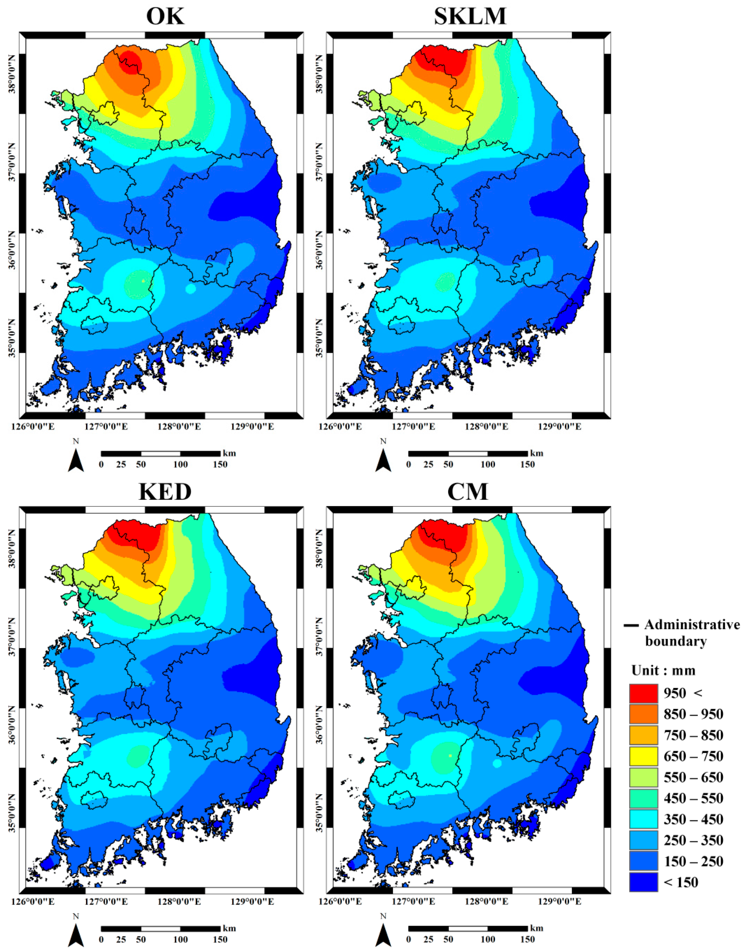
4.2. Prediction Results

Three multivariate kriging algorithms were applied using GSLIB [44] and FORTRAN programming. As four different rain gauge density scenarios were applied, the different numbers of rain gauges were used to compute kriging weights by considering the maximum number of each scenario and the correlation ranges of variogram models. As a reference for the spatial distributions obtained by integration, the downscaled TRMM precipitation estimates were first integrated with all 71 rain gauges (i.e., S100). Figure 5 shows histograms of the regression coefficients (intercept and slope) for KED in July. The regression coefficients were locally re-estimated by the KED system, so their values constitute distributions, rather than a single value in SKLM, and thus, the local trends varied across the study area.

Figure 6 presents four prediction results on a 1-km pixel generated by OK using all of the rain gauge data (S100) and three multivariate kriging algorithms for July. When comparing the ATP kriging estimates in Figure 4a with the OK estimates from the rain gauge data, the overall patterns were similar with a large amount of precipitation in the northern part and a small amount of precipitation in the southern and eastern parts. However, overestimated patterns in the downscaled TRMM precipitation estimates were observed in the northeastern and eastern parts, as indicated by the positive rME value in Table 1. Since rME is an overall location-independent measure of bias, locally different patterns may be observed. The relatively large value in the southwestern part of the study area in the OK estimates was not observed in the downscaled TRMM precipitation in Figure 4a. After integrating the rain gauge data, the local pattern, which was not observed in the downscaled TRMM precipitation, could be reproduced in all results by three multivariate kriging algorithms. According to a visual inspection, similar precipitation patterns were presented in all of the prediction results when using all 71 rain gauges, which indicates that the rain gauge data greatly affected the prediction results, and the predictive performance should be assessed under different rain gauge density scenarios.

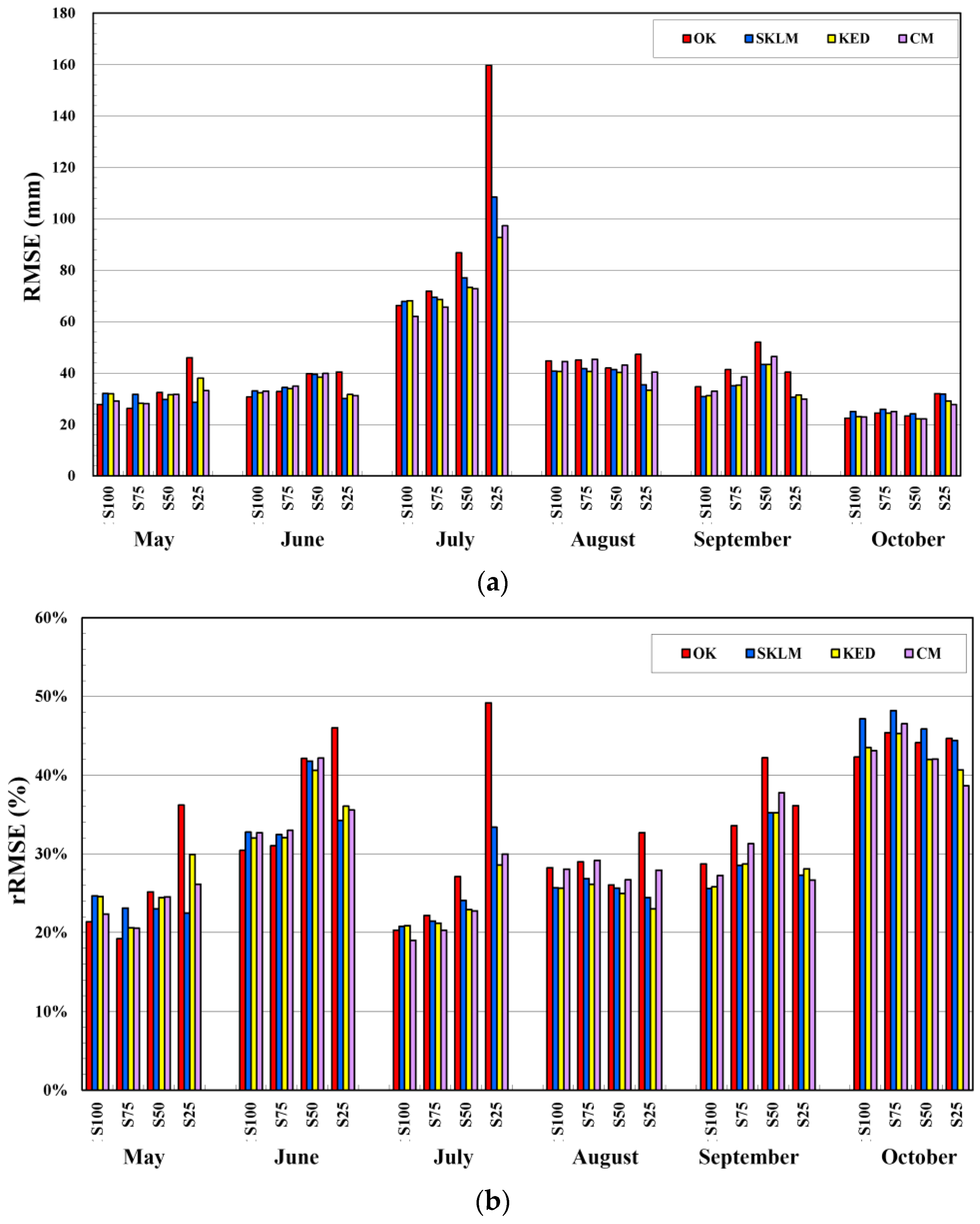
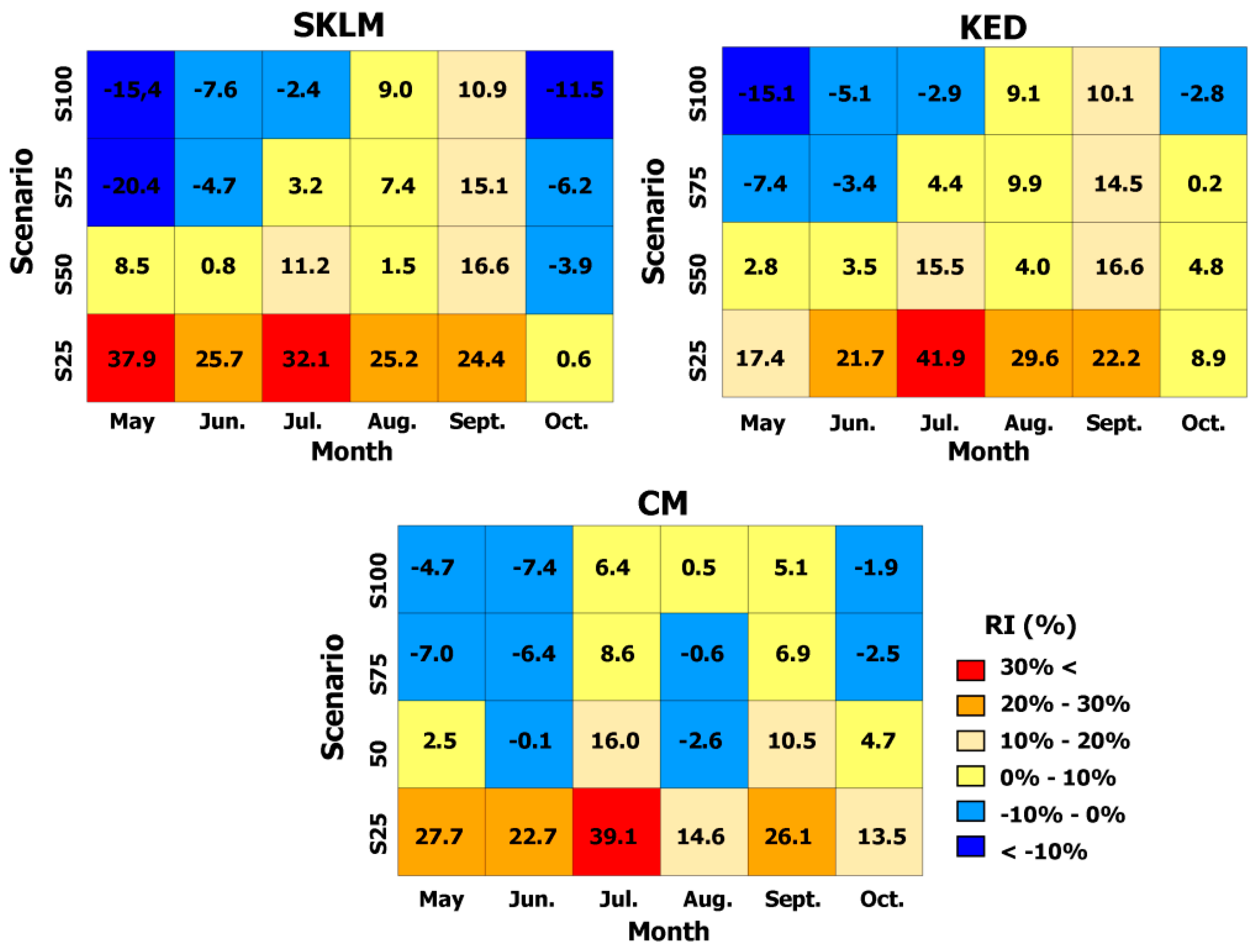
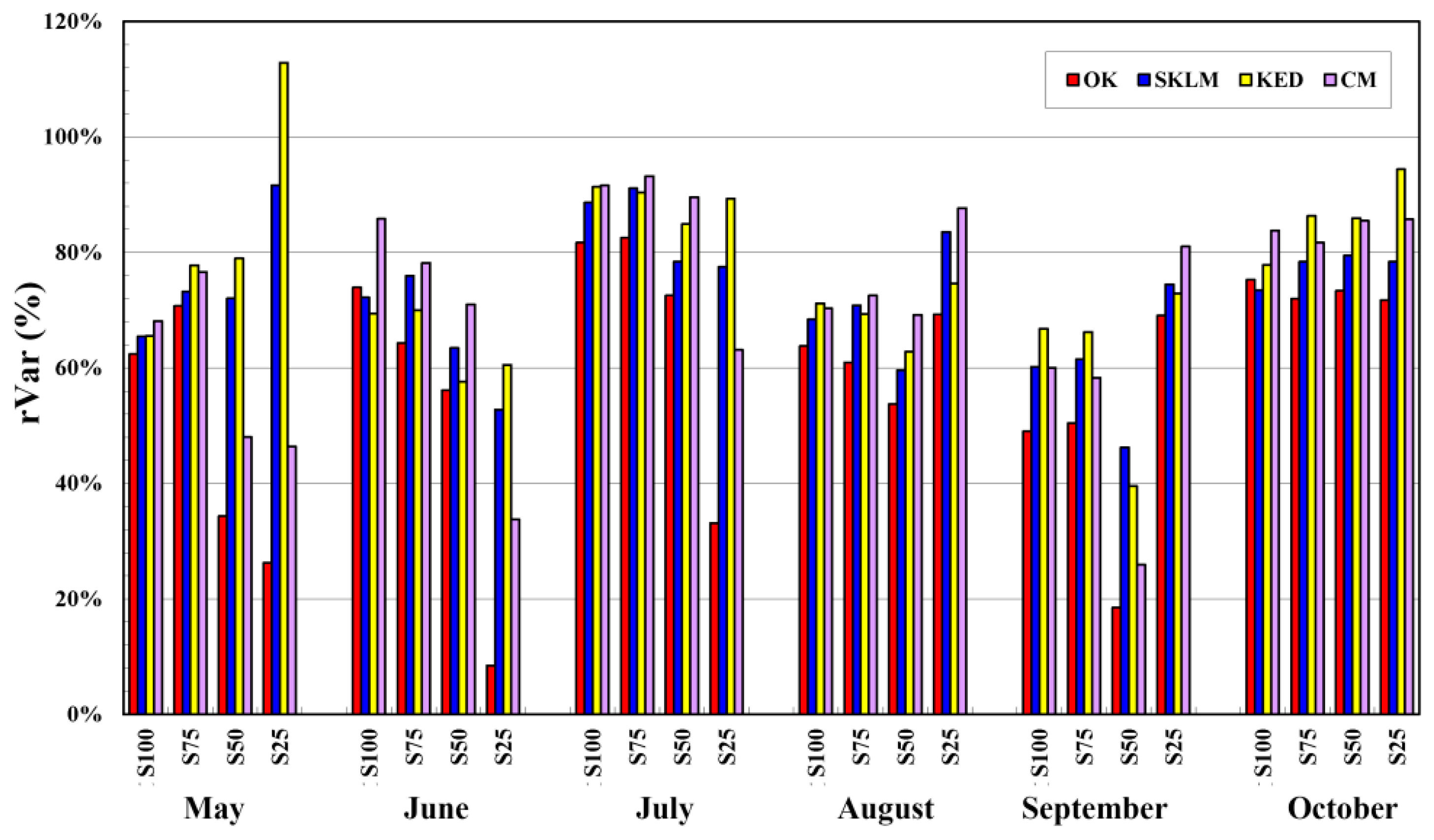
4.3. Performance Evaluation Results

LOO CV was applied to the different rain gauge density scenarios. For an objective comparison, regression and residual kriging for SKLM were applied to the rain gauge data used in each scenario, rather than using the regression model with all of the rain gauge data.

The average error statistics for all months are summarized in

Table 2. Average precipitation error statistics for all months obtained from different kriging algorithms in different rain gauge density scenarios. RI, relative improvement index.

Statistics	Scenario	OK	SKLM	KED	CM
rME (%)	S100	0.14	0.08	0.66	0.06
	S75	0.39	0.43	0.27	0.18
	S50	0.33	0.09	−0.01	0.23
	S25	−0.39	−0.40	−0.13	−0.03
rRMSE (%)	S100	28.55	29.43	28.73	28.74
	S75	30.05	30.09	28.99	30.12
	S50	34.45	32.59	31.69	32.66
	S25	40.80	31.03	31.04	30.81
rVar (%)	S100	67.69	71.39	73.68	76.62
	S75	66.81	75.17	76.67	76.76
	S50	51.45	66.55	68.30	64.87
	S25	46.32	76.39	84.11	66.29
RI of RMSE (%)	S100	-	−2.84	−1.11	−0.33
	S75	-	−0.92	3.04	−0.17
	S50	-	5.78	7.87	5.18
	S25	-	24.30	23.62	23.95

. As the rain gauge density decreased, the bias slightly increased, and underestimation (i.e., negative rME) was dominant in all the predictions for S25. Comparisons of the rRMSE values for all of the predictions showed that integrating TRMM precipitation data with the rain gauges did not yield any significant improvements in RMSE when many rain gauges were used for prediction. In particular, OK was the best predictor when all of the rain gauges were used (S100). When few rain gauges were used (S50 and S25), however, all of the multivariate kriging algorithms outperformed OK. The impact of the amount of rain gauges was the most striking in S25. All of the multivariate kriging algorithms yielded significant improvements in RMSE (more than 23%) for S25, compared with OK. It was not possible to conclude which of the three algorithms was the best predictor. KED had the best prediction performance for S75 and S50, whereas SKLM and CM were the best for S25 and S100, respectively. When comparing the rVar values that indicate the degree of smoothness, OK was greatly affected by the rain gauge density. The decrease of the rain gauge density increased the smoothing effect for OK. Even though many rain gauges were integrated with TRMM precipitation product, the rVar values were greater for all of the multivariate kriging algorithms than OK, thereby implying that the TRMM precipitation product contributed to greater variations in the predicted precipitation. When very few rain gauges were used (S25), KED had the lowest smoothness. Overall, KED and SKLM obtained lower levels of smoothness than CM.

The error statistics per month were further analyzed to investigate the monthly variations in such statistics based on different kriging algorithms. rME did not show any interpretable patterns for each month. Comparing the monthly variations in the RMSEs with different kriging algorithms (Figure 7a), the RMSE was highest in July with a relatively large amount of precipitation. The OK prediction for July had the highest RMSE of 159.7 mm. As the density of the rain gauges decreased, the RMSE of OK increased for all months. By contrast, the three multivariate kriging algorithms had similar or lower RMSEs compared with OK as the density of rain gauges decreased. In particular, for S25, integration with the TRMM precipitation product improved the RMSE compared with OK.

The monthly variations in the RMSEs were further analyzed by comparing the rRMSE values (Figure 7b). The largest RMSEs were obtained in July, whereas the rRMSEs were relatively larger in October. The relatively lower RMSEs in October were due to the lower amount of precipitation in October. The larger rRMSEs indicate that the prediction results for October were relatively unreliable compared with other months. Similar to the RMSE, the improvement in the rRMSE brought by the integration of rain gauge and TRMM precipitation data was also significant for S25. In addition, the period from August–October had lower rRMSEs, although very few rain gauges were used (e.g., S25).

The relative improvements in the RMSE over OK are presented as a contingency table plot in Figure 8, where the blue color denotes that the RMSEs of the multivariate kriging algorithms are higher than that for OK, thereby implying its poor predictive performance. When a large number of rain gauges was used for integration with the TRMM data (i.e., S100), no significant improvements in the predictive performance could be obtained. In some months such as May, integration with the TRMM data led to even larger errors compared with OK. As the density of rain gauges decreased, however, the contribution of the TRMM data increased and led to significant improvements in the predictive performance for all months. All three integration algorithms performed better than OK with S50 and S25, except for August and September. The largest improvement in the RMSE was obtained in most months with S25, except for October. This result confirms that the contribution of TRMM precipitation is the greatest when fewer rain gauges are used. A comparison of the predictive performance of the three integration algorithms showed that SKLM improved the RMSE most for May (37.9%), as well as KED for June (41.9%) and CM for September (26.1%). The relatively lower improvement in the RMSE for October might be explained by the errors in TRMM precipitation product. As shown in Table 1, the rRMSE of TRMM was highest in October. Thus, the integration with the TRMM precipitation product containing errors led to no significant improvements in the RMSE when fewer rain gauges were used. According to the three error statistics, the predictive performance when integrating the TRMM precipitation product with rain gauge data depends greatly on the density of rain gauges. Thus, the integration of TRMM precipitation data is only beneficial when the number of available rain gauges is relatively small.

The variations of rVar that measures the degree of smoothness for predictions are shown in Figure 9. The smoothing effect of OK increased dramatically as the density of rain gauges decreased in all months. By contrast, integrating TRMM precipitation data using multivariate kriging greatly reduced the smoothing effect. In some months such as May, September and October, the rVar value increased for KED although a very small number of rain gauges was used (S25). A comparison of the multivariate kriging algorithms showed that KED had larger rVar values for most months and densities compared with SKLM and CM. When considering all of the RMSE, rRMSE and rVar, it is confirmed again that the benefit of using TRMM precipitation data is most apparent as the density of rain gauges decreases.

Overall, these comparison results for different rain gauge density scenarios reveal that the advantage of integrating coarse resolution satellite precipitation products with rain gauges is not striking when many rain gauges are available. If the geostatistical downscaling-integration approach is applied to other areas where there are very few rain gauges relative to the size of the area, however, integrating the coarse resolution satellite precipitation products with rain gauges could be beneficial, thereby highlighting the necessity of using the satellite precipitation products.

5. Discussion

To further investigate the differences among the three multivariate kriging algorithms, we computed correlation coefficients by comparing error statistics and predictions for different inputs and algorithms using all of the months and densities (

Table 3. Summary of correlation coefficients from the comparison with error statistics and predictions for different kriging algorithms.

Case	SKLM	KED	CM
(a) Comparison with TRMM error statistics and predictions
rRMSE for TRMM precipitation versus rRMSE for kriging predictions	0.96	0.95	0.92
Average of correlation of TRMM precipitation versus kriging predictions	0.97	0.95	0.92
(b) Comparison with OK error statistics and predictions
rRMSE for OK predictions versus rRMSE for kriging predictions	0.80	0.81	0.85
Average of correlation for OK predictions versus kriging predictions	0.90	0.90	0.93

). Since error statistics obtained from all months were used in the computations, the rRMSEs were used as error statistics instead of the RMSEs. First, the impact of TRMM precipitation data on the predictive performance of each multivariate kriging algorithm was analyzed. The errors in the TRMM precipitation had a strong positive correlation with the predictive performance for all three algorithms (Table 3a). A strong positive correlation was also observed in the average of correlation coefficients between the TRMM precipitation data and the predicted values by each multivariate kriging algorithm for all months and densities. Strong correlations were obtained by all three algorithms, but SKLM and KED had relatively stronger correlations than CM. For merging rain gauge and radar data using KED, similar findings were obtained by Berndt et al. [28], where KED was more sensitive to the radar data quality than CM. These measures indicate that the gain of integrating TRMM precipitation with rain gauges depends on the errors or quality of the TRMM precipitation data, as well as on the density of the rain gauges.

To analyze the differences of predictions without or with the integration of the TRMM precipitation product, the error statistics and predictions obtained by OK were compared with those obtained using multivariate kriging algorithms (Table 3b). The correlation between the rRMSEs for OK and each multivariate kriging algorithm was also strong. In addition, the average correlation coefficients between the OK predictions and the predicted values by each multivariate kriging were also very strong. All of the multivariate kriging algorithms had high correlation, but CM had the largest correlation coefficients, unlike the analysis result regarding the impact of errors in the TRMM precipitation data. These differences in the impact analysis results may be explained by the characteristics of each multivariate kriging algorithm. In SKLM and KED, soft data contribute to the estimation of the local means. The errors in the soft data are adjusted using hard data, but they might not be fully adjusted. Residuals are the main target of kriging in SKLM and KED, so their dependency on the local means also affects the prediction results. Meanwhile, CM predictions are the sum of the contributions from both the hard and soft data. When few rain gauges are used for CM, the errors in the OK predictions may greatly affect the final CM predictions. Based on these findings, the impacts of errors in the OK predictions may be reduced if the correlation with the OK predictions is low, but that with the TRMM precipitation data is large. For example, the CM predictions for S25 in June had a correlation coefficient of 0.45 with the OK predictions, but 0.948 with the TRMM precipitation data. Thus, the RMSE of the CM predictions (31.44) was smaller than that of the OK predictions (40.44). However, intrinsic errors in the TRMM precipitation data may also have degraded the CM predictions. Thus, the tentative conclusions obtained from this study should be evaluated extensively from experiments using longer time-series datasets.

In relation to integrating datasets measured over different supports, advanced geostatistical kriging algorithms, which integrate datasets from different supports within one stage unlike our two-stage approach, have been proposed. Liu and Journel [45] proposed block kriging to integrate well-logging data with coarse scale geophysical exploration data. Goovaerts [46] also proposed area-and-point kriging as a general framework for combining point- and areal-support data and demonstrated its effectiveness through case studies in the fields of soil science and medical geography. From impact analysis results in this study, it was observed that the reliability of the integration of coarse resolution satellite-derived precipitation estimates with rain gauges was still susceptible to errors in areal-support data. Since the variants of conventional kriging directly integrate data measured over different supports, intrinsic errors in the areal-support data may propagate to the integration procedure, thereby yielding unreliable final prediction results at a fine spatial resolution. If a priori information is available regarding the error variance, this information could be used to adjust the kriging weights [45,47]. However, information on the error variance is not always available. Thus, the final prediction results obtained by direct integration without error adjustment may be affected severely by the errors in the areal-support data. To prove this statement, the two-stage approach presented in this study should be compared with the direct integration approach.

In order to focus on the benefit of integrating coarse resolution satellite-derived precipitation estimates with rain gauge data, other environmental variables related to precipitation were not considered in this study. If auxiliary environmental variables at a fine spatial resolution are available, they can easily be integrated within the geostatistical framework presented in this study. These days, many fine scale auxiliary variables, such as DEM and the vegetation index, can be readily obtained from satellites (e.g., ASTER DEM and MODIS products). These auxiliary variables can be integrated in either (1) the downscaling step or (2) the integration step. If auxiliary variables at a fine spatial resolution are used during the downscaling step, several downscaling methods mentioned in the Introduction Section (e.g., linear regression-ATP residual kriging [4] and geographically-weighted regression-spline interpolation of residuals [15,19]) can be employed to generate the satellite-derived precipitation estimates while accounting for the spatial heterogeneity at a fine spatial resolution. As discussed in Park et al. [17], however, the benefit of incorporating fine resolution auxiliary variables for downscaling may be not always great in some cases, when compared with downscaling without the auxiliary variables. In addition, any regression model with higher explanatory power does not always lead to an improvement of predictive performance due to the intrinsic errors of input coarse resolution data [48]. If the downscaled satellite-derived precipitation estimates with the fine resolution auxiliary variables are integrated with rain gauge data, the final prediction results at the fine resolution might not show improved performance in some areas with sparse rain gauges. The second possible integration approach is to use the auxiliary variables at the fine resolution as additional inputs for multivariate kriging algorithms as in this study. SKLM is more efficient than other multivariate kriging algorithms because many auxiliary variables can be used to estimate the local means via multiple linear/non-linear regression modeling. Meanwhile, KED is only applicable when the auxiliary variables are linearly related to precipitation. It also becomes computationally demanding when many auxiliary variables are integrated. CM has been applied to integrate only one type of radar or satellite precipitation product, so the applicability of CM is not clear. By considering these issues, thus, integrating datasets from both different supports and multiple sources should be tested extensively in future research.

Another important issue in downscaling and integration is to quantify the uncertainty attached to prediction. In particular, the uncertainty quantification or assessment in downscaling of coarse resolution satellite product is very important because downscaling is regarded as an under-determined inverse problem [4]. In downscaling of the coarse resolution satellite product, the uncertainty can be assessed within a stochastic simulation framework [4,39,49]. The multiple downscaled realizations from stochastic simulation can be used as inputs of multivariate kriging for integration with rain gauge data. Subsequently, the comparison of the differences between multiple integration results can be used to quantify the uncertainty or impact of downscaled satellite-derived precipitation estimates on, say, hydrological assessments. As the downscaled satellite-derived precipitation estimates are integrated with rain gauge data, however, there are several different sources of uncertainty at ungauged locations, such as the spatial configuration of rain gauges and spatial correlation structures of the residuals, as well as the uncertainty of the downscaled satellite-derived precipitation estimates. Due to the complexity of considering all different sources of uncertainty, uncertainty assessment based on stochastic simulation was not considered in this study. A stochastic simulation framework for downscaling (conditional ATP simulation [36]) and integration (multivariate conditional simulation [39]) has already been established in geostatistics. Thus, the two-stage geostatistical kriging approach presented in this paper could be extended to the stochastic simulation framework for target-specific uncertainty assessment, such as the impact of the incorporation of fine resolution auxiliary variables on the downscaling of coarse resolution satellite precipitation products.

6. Conclusions

The benefits of integrating coarse resolution satellite-derived precipitation data with rain gauge data have been investigated for fine resolution mapping of precipitation. For this purpose, a two-stage geostatistical downscaling approach was presented for integrating datasets from different supports and adjusting the errors in the satellite precipitation product. A case study using TRMM 3B43 monthly precipitation products obtained in South Korea demonstrated that integrating the TRMM precipitation product with rain gauge data did not improve the predictive performance with a large number of rain gauges, but the integration was increasingly beneficial as the density of rain gauges decreased. In addition, integrating the TRMM precipitation data could generate more variable precipitation at a fine resolution with less smoothing effect, compared with the OK predictions using only rain gauge data. Thus, the effectiveness of coarse resolution satellite precipitation products is therefore more pronounced when high resolution mapping of precipitation is required for areas with sparse rain gauges. The predictive performance of all multivariate kriging algorithms was affected by errors in the TRMM precipitation product. To support the findings obtained in this study, the impact of errors in input coarse resolution data on the predictive performance of integration results via stochastic simulation will be investigated in future research.

References

1. Kyriakidis, P.C.; Miller, N.L.; Kim, J. Uncertainty propagation of regional climate model precipitation forecasts to hydrologic impact assessment. J. Hydrometeorol. 2001, 2, 140–160. [Google Scholar] [CrossRef]
2. Kyriakidis, P.C.; Kim, J.; Miller, N.L. Geostatistical mapping of precipitation from rain gauge data using atmospheric and terrain characteristics. J. Appl. Meteor. 2001, 40, 1855–1877. [Google Scholar] [CrossRef]
3. Goovaerts, P. Geostatistical approaches for incorporating elevation into the spatial interpolation of rainfall. J. Hydrol. 2000, 228, 113–129. [Google Scholar] [CrossRef]
4. Park, N.-W. Spatial downscaling of TRMM precipitation using geostatistics and fine scale environmental variables. Adv. Meteorol. 2013, 2013, 237126. [Google Scholar] [CrossRef]
5. Atlas, D. Radar in Meteorology; Springer: New York, NY, USA, 1990. [Google Scholar]
6. Hong, Y.; Gourley, J.J. Radar Hydrology: Principles, Models, and Applications; CRC Press: Boca Raton, FL, USA, 2014. [Google Scholar]
7. Seo, D.-J.; Breidenbach, J.P.; Johnson, E.R. Real-time estimation of mean field bias in radar rainfall data. J. Hydrol. 1999, 3–4, 131–147. [Google Scholar] [CrossRef]
8. Ciach, G.J.; Krajewski, W.F.; Villarini, G. Product-error-driven uncertainty model for probabilistic precipitation estimation with NEXRAD data. J. Hydrometeorol. 2007, 8, 1325–1347. [Google Scholar] [CrossRef]
9. Kummerow, C.D.; Barnes, W.; Kozu, T.; Shiue, J.; Simpson. The tropical rainfall measuring mission (TRMM) sensor package. J. Atmos. Ocean. Tech. 1998, 15, 809–817. [Google Scholar] [CrossRef]
10. Imaoka, K.; Kachi, M.; Fujii, H.; Murakami, H.; Hori, M.; Ono, A.; Igarashi, T.; Nakagawa, K.; Oki, T.; Honda, Y.; et al. Global change observation mission (GCOM) for monitoring carbon, water cycles, and climate change. Proc. IEEE 2010, 98, 717–734. [Google Scholar] [CrossRef]
11. Hou, A.Y.; Kakar, R.K.; Neeck, S.; Azarbarzin, A.A.; Kummerow, C.D.; Kojima, M.; Oki, R.; Nakamura, K.; Iguchi, T. The global precipitation measurement mission. Bull. Am. Meteorol. Soc. 2014, 95, 701–722. [Google Scholar] [CrossRef]
12. Atkinson, P.M. Downscaling in remote sensing. Int. J. Appl. Earth Obs. Geoinf. 2013, 22, 106–114. [Google Scholar] [CrossRef]
13. Immerzeel, W.W.; Rutten, M.M.; Droogers, P. Spatial downscaling of TRMM precipitation using vegetative response on the Iberian Peninsula. Remote Sens. Environ. 2009, 113, 362–370. [Google Scholar] [CrossRef]
14. Jia, S.; Zhu, W.; Lü, A.; Yan, T. A statistical spatial downscaling algorithm of TRMM precipitation based on NDVI and DEM in the Qaidam basin of China. Remote Sens. Environ. 2011, 115, 3069–3079. [Google Scholar] [CrossRef]
15. Chen, F.; Liu, Y.; Liu, Q.; Li, X. Spatial downscaling of TRMM 3B43 precipitation considering spatial heterogeneity. Int. J. Remote Sens. 2014, 35, 3074–3093. [Google Scholar] [CrossRef]
16. Shi, Y.; Song, L.; Xia, Z.; Lin, Y.; Myneni, R.B.; Choi, S.; Wang, L.; Ni, X.; Lao, C.; Yang, F. Mapping annual precipitation across mainland China in the period 2001–2010 from TRMM 3B43 product using spatial downscaling approach. Remote Sens. 2015, 7, 5849–5878. [Google Scholar] [CrossRef]
17. Park, N.-W.; Hong, S.; Kyriakidis, P.C.; Lee, W.; Lyu, S.-J. Geostatistical downscaling of AMSR2 precipitation with COMS infrared observations. Int. J. Remote Sens. 2016, 37, 3858–3869. [Google Scholar] [CrossRef]
18. Jing, W.; Yang, Y.; Yue, X.; Zhao, X. A spatial downscaling algorithm for satellite-based precipitation over the Tibetan plateau based on NDVI, DEM, and land surface temperature. Remote Sens. 2016, 8, 655. [Google Scholar] [CrossRef]
19. Chen, C.; Zhao, S.H.; Duan, Z.; Qin, Z.H. An improved spatial downscaling procedure for TRMM 3B43 precipitation product using geographically weighted regression. IEEE J. Sel. Top. Appl. Earth Obs. Remote Sens. 2015, 8, 4592–4604. [Google Scholar] [CrossRef]
20. Xu, S.; Wu, C.; Wang, L.; Gonsamo, A.; Shen, Y.; Niu, Z. A new satellite-based monthly precipitation downscaling algorithm with non-stationary relationship between precipitation and land surface characteristics. Remote Sens. Environ. 2015, 162, 119–140. [Google Scholar] [CrossRef]
21. Huffman, G.J.; Bolvin, D.T.; Nelkin, E.J.; Wolff, D.B.; Adler, R.F.; Gu, G.; Hong, Y.; Bowman, K.P.; Stocker, E.F. The TRMM multisatellite precipitation analysis (TMPA): Quasi-global, multiyear, combined-sensor precipitation estimates at fine scale. J. Hydrometeorol. 2007, 8, 38–55. [Google Scholar] [CrossRef]
22. Nerini, D.; Zulkafli, Z.; Wang, L.-P.; Onof, C.; Buytaert, W.; Lavado-Casimiro, W.; Guyot, J.-L. A comparative analysis of TRMM-rain gauge data merging techniques at the daily time scale for distributed rainfall-runoff modeling applications. J. Hydrometeorol. 2015, 16, 2153–2168. [Google Scholar] [CrossRef]
23. Porcù, F.; Milani, L.; Petracca, M. On the uncertainties in validating satellite instantaneous rainfall estimates with raingauge operational network. Atmos. Res. 2014, 144, 73–81. [Google Scholar] [CrossRef]
24. Li, M.; Shao, Q. An improved statistical approach to merge satellite rainfall estimates and raingauge data. J. Hydrol. 2010, 385, 51–64. [Google Scholar] [CrossRef]
25. Todini, E. A Bayesian technique for conditioning radar precipitation estimates to rain-gauge measurements. Hydrol. Earth Syst. Sci. 2001, 5, 187–199. [Google Scholar] [CrossRef]
26. Baik, J.; Park, J.; Ryu, D.; Choi, M. Geospatial blending to improve spatial mapping of precipitation with high spatial resolution by merging satellite-based and ground-based data. Hydrol. Process. 2016, 30, 2789–2803. [Google Scholar]
27. Chappell, A.; Renzullo, L.J.; Raupach, T.H.; Haylock, M. Evaluating geostatistical methods of blending satellite and gauge data to estimate near real-time daily rainfall for Australia. J. Hydrol. 2013, 493, 105–114. [Google Scholar] [CrossRef]
28. Berndt, C.; Rabiei, E.; Haberlandt, U. Geostatistical merging of rain gauge and radar data for high temporal resolutions and various station density scenarios. J. Hydrol. 2014, 508, 88–101. [Google Scholar] [CrossRef]
29. Erdin, R.; Frei, C.; Küsch, H.R. Data transformation and uncertainty in geostatistical combination of radar and rain gauges. J. Hydrometeorol. 2012, 13, 1332–1346. [Google Scholar] [CrossRef]
30. Goudenhoofdt, E.; Delobbe, L. Evaluation of radar-gauge merging methods for quantitative precipitation estimates. Hydrol. Earth Syst. Sci. 2009, 13, 195–203. [Google Scholar] [CrossRef]
31. Hunink, J.E.; Immerzeel, W.W.; Droogers, P. A high-resolution precipitation 2-step mapping procedure (HiP2P): development and application to a tropical mountainous area. Remote Sens. Environ. 2014, 140, 179–188. [Google Scholar] [CrossRef]
32. Duan, Z.; Bastiaanssen, W.G.M. First results from version 7 TRMM 3B43 precipitation product in combination with a new downscaling-calibration procedure. Remote Sens. Environ. 2013, 131, 1–13. [Google Scholar] [CrossRef]
33. Kyriakidis, P.C. A geostatistical framework for area-to-point spatial interpolation. Geogr. Anal. 2004, 36, 259–289. [Google Scholar] [CrossRef]
34. Korea Meteorological Administration. Available online: http://web.kma.go.kr/eng/biz/climate_01.jsp (accessed on 31 January 2017).
35. Oh, H.-J.; Sohn, B.-J.; Smith, E.A.; Turk, F.J.; Seo, A.-S.; Chung, H.-S. Validating infrared-based rainfall retrieval algorithms with 1-minute spatially dense raingage measurements over Korean peninsula. Meteorol. Atmos. Phys. 2002, 81, 273–287. [Google Scholar] [CrossRef]
36. Kyriakidis, P.C.; Yoo, E.H. Geostatistical prediction and simulation of point values from areal data. Geogr. Anal. 2005, 37, 124–151. [Google Scholar] [CrossRef]
37. Goovaerts, P. Kriging and semivariogram deconvolution in the presence of irregular geographical units. Math. Geosci. 2008, 40, 101–128. [Google Scholar] [CrossRef]
38. Hengl, T.; Heuvelink, G.B.M.; Stein, A. A generic framework for spatial prediction of soil variables based on regression-kriging. Geoderma 2004, 120, 75–93. [Google Scholar] [CrossRef]
39. Goovaerts, P. Geostatistics for Natural Resources Evaluation; Oxford University Press: New York, NY, USA, 1997. [Google Scholar]
40. Patriarche, D.; Castro, M.C.; Goovaerts, P. Estimating regional hydraulic conductivity fields-a comparative study of geostatistical methods. Math. Geol. 2005, 37, 587–613. [Google Scholar] [CrossRef]
41. Sales, M.H.; Souza, C.M., Jr.; Kyriakidis, P.C. Fusion of MODIS images using kriging with external drift. IEEE Trans. Geosci. Remote Sens. 2013, 51, 2250–2259. [Google Scholar] [CrossRef]
42. Ehret, U. Rainfall and Flood Nowcasting in Small Catchments Using Weather Radar. Ph.D. Thesis, University of Stuttgart, Stuttgart, Germany, 2002. [Google Scholar]
43. Sinclair, S.; Pegram, G. Combining radar and rain gauge rainfall estimates using conditional merging. Atmos. Sci. Lett. 2005, 6, 19–22. [Google Scholar] [CrossRef]
44. Deutsch, C.V.; Journel, A.G. GSLIB: Geostatistical Software Library and User’s Guide, 2nd ed.; Oxford University Press: New York, NY, USA, 1998. [Google Scholar]
45. Liu, Y.; Journel, A.G. A package for geostatistical integration of coarse and fine scale data. Comput. Geosci. 2009, 35, 527–547. [Google Scholar] [CrossRef]
46. Goovaerts, P. Combining areal and point data in geostatistical interpolation: Applications to soil science and medical geography. Math. Geosci. 2010, 42, 535–554. [Google Scholar] [CrossRef] [PubMed]
47. Remy, N.; Boucher, A.; Wu, J. Applied Geostatistics with SGeMS: A User’s Guide; Cambridge University Press: Cambridge, UK, 2009. [Google Scholar]
48. Park, N.-W. Spatial downscaling of coarse scale satellite products: State-of-the-arts and issues. In Proceedings of the Fall Meeting of Korean Society of Remote Sensing, Chungjoo, Korea, 4 November 2016; pp. 310–311. (In Korean)
49. Gires, A.; Tchiguirinskaia, I.; Schertzer, D.; Schellart, A.; Berne, A.; Lovejoy, S. Influence of small scale rainfall variability on standard comparison tools between radar and rain gauge data. Atmos. Res. 2014, 138, 125–138. [Google Scholar] [CrossRef]
Figure 1. Location of automated synoptic observing systems (ASOS) data (black dots) over the TRMM 3B43 precipitation product obtained in July 2013. The polylines are administrative boundaries in South Korea.
Remotesensing 09 00255 g001
Figure 2. Graphical depiction of the geostatistical downscaling and integration approach presented in this study.
Remotesensing 09 00255 g002
Figure 3. Location of rain gauges (blue dots) in different density scenarios. The number in parentheses for each scenario denotes the number of rain gauges. S75, scenario 75% sampling density.
Remotesensing 09 00255 g003
Figure 4. (a) Downscaling result by area-to-point (ATP) kriging for July in 2013; and (b) scatter-plot of the original TRMM precipitation values versus the average of ATP kriging results within each 25-km TRMM pixel.
Remotesensing 09 00255 g004
Figure 5. Histograms of the regression coefficients of kriging with an external drift (KED) for July. The black dot in the box-plot under each histogram denotes the global regression coefficient of simple kriging with local means (SKLM).
Remotesensing 09 00255 g005
Figure 6. Precipitation prediction results for July using different kriging algorithms. OK, ordinary kriging; CM, conditional merging.
Remotesensing 09 00255 g006
Figure 7. Monthly precipitation error statistics for various prediction algorithms in different rain gauge density scenarios: (a) RMSE; and (b) rRMSE.
Remotesensing 09 00255 g007
Figure 8. Contingency plot of RI for the three multivariate kriging algorithms in each month and the density of rain gauges. The numerical value in each cell represents the RI value for the corresponding month and scenario.
Remotesensing 09 00255 g008
Figure 9. Monthly variations in rVar for the kriging algorithms in different rain gauge density scenarios.
Remotesensing 09 00255 g009