Mapping Rice Fields in Urban Shanghai, Southeast China, Using Sentinel-1A and Landsat 8 Datasets

Abstract

Sentinel-1A and Landsat 8 images have been combined in this study to map rice fields in urban Shanghai, southeast China, during the 2015 growing season. Rice grown in paddies in this area is characterized by wide inter-field variability in addition to being fragmented by other land-uses. Improving rice classification accuracy requires the use of multi-source and multi-temporal high resolution data for operational purposes. In this regard, we first exploited the temporal backscatter of rice fields and background land-cover types at the vertical transmitted and vertical received (VV) and vertical transmitted and horizontal received (VH) polarizations of Sentinel-1A. We observed that the temporal backscatter of rice increased sharply at the early stages of growth, as opposed to the relatively uniform temporal backscatter of the other land-cover classes. However, the increase in rice backscatter is more sustained at the VH polarization, and two-class separability measures further indicated the superiority of VH over VV in discriminating rice fields. We have therefore combined the temporal VH images of Sentinel-1A with the normalized difference vegetation index (NDVI) and the modified normalized difference water index (MNDWI) derived from a single-date cloud-free Landsat 8 image. The integration of these optical indices with temporal backscatter eliminated all commission errors in the Rice class and increased overall accuracy by 5.3%, demonstrating the complimentary role of optical indices to microwave data in mapping rice fields in subtropical and urban landscapes such as Shanghai.

1. Introduction

Urban and peri-urban agriculture (UPA) has gained much recognition as a major source of livelihoods for inhabitants within cities and those along the rural–urban fringe, especially in developing countries [1,2,3]. The increasing trends of rural–urban migration have triggered a population explosion in cities. Migrated rural surplus labor is mostly unskilled. As a result, migrant populations mainly engage in primary economic activities, prominent among which is farming [4].

The concept of UPA is fraught with definitional challenges as it involves a diverse range of agricultural activities involving crops, livestock, and aquaculture at scales ranging from roof-top gardens to larger cultivated open spaces [5]. Additionally, the boundary between the urban and peri-urban is along a land-use continuum which exhibits considerable heterogeneity [6]. Various definitions of UPA have been put forward by scholars, and at the center of all these definitions is the understanding that urban agriculture is farming practiced in inner city areas. On the other hand, peri-urban agriculture is a residual form of farming at the fringes of growing cities, though a commonly agreed spatial definition is missing [5]. The peri-urban is a transition zone between rural and urban areas, which on the one hand is characterized by lower population density and inadequate infrastructure compared to cities, and therefore not “urban”, and on the other hand a limited amount of agricultural and natural land, and therefore not “rural” [7,8]. While urban agriculture primarily meets food demands at household levels, peri-urban agriculture provides larger quantities with broader distribution pathways, giving it a separate status in terms of food security planning [5]. Food security is one major objective in the millennium development goals.

Urban agriculture is an important land-use and economic activity central to millions of people in the world. It contributes significantly in meeting the nutritional requirements of urban dwellers and hence, improves urban food security [9,10]. According to [11,12], urban agriculture supplies food to about one-quarter of the world’s urban population. Apart from enhancing food security and urban incomes, urban farming also contributes to flood control, land reclamation and city greening [13,14]. Hence, the economic and environmental significance of urban agriculture are enormous.

However, despite the enormous social, economic and environmental benefits provided by urban agriculture, land is increasingly becoming scarce for the sustainability of this vital sector [3,15]. Residential and industrial land-uses are ever expanding into arable land at the fringes of urban centers [4]. The unprecedented population increase in cities, especially in the developing world, means more living space will be required for housing and other social infrastructure. This has led to a gradual loss and fragmentation of agricultural land-use in urban and peri-urban areas [16,17], and one of the most important agricultural crops affected by this socio-economic transformation is rice [18].

Rice is one of the most important food crops and accounts for 20% of the world’s calorie supply. Rice is regarded the most important food for the poor as it serves as staple for about a billion people subsisting on less than a dollar a day [19]. The rice crop is extensively grown in upland and lowland ecologies found in the tropics, sub-tropics and temperate regions in Asia, Africa, Australia, Europe and the Americas. Irrigation is often practiced in places where rain-fed agriculture is infeasible [20].

The continuous increase in the world’s human population has triggered an increase in the demand for rice especially in developing countries, where rice is a major component of the daily diet. In response to such food demands, several calls have been made over the years to increase rice production [21]. However, such efforts have been hindered by the substantial shift in investment of major rice producing countries from agriculture to manufacturing, and the continuous conversion of agricultural land to residential and industry, mostly as a consequence of growing urbanization and industrialization. Additionally, urban agricultural land-uses such as vegetable gardening, fruit farming and aquaculture are increasingly encroaching into lands initially dedicated to rice farming. Globally, there is an increasing decline in rice planted areas [22] and the intensification of this trend in urban and peri-urban areas could have implications for global food security and food self-sufficiency. However, the loss of paddy rice area has occurred in tandem with intensification of rice farming through the use of agrochemicals to control pest and improve soil fertility, introduction of improved (short cycle and high yielding) varieties and mechanized agriculture.

Monitoring rice cultivation is of great significance as such statistics could provide a means of early warning signals of food scarcity, and hence, supporting food security policies [23]. Perhaps the most widely and easily monitored variable of rice cultivation is acreage. Under the assumption of ceteris paribus (all other things being equal), an increase in the rice planted area should translate to an increase in rice productivity and food supply. Rice fields have also been noted to be major sources of methane, a notable green house gas [24]. Monitoring paddy rice fields is therefore of much relevance in understanding the global dynamics of greenhouse gas emissions, rising temperatures and climate change. Additionally, one of the most potent impacts of climate change is dwindling water resources [25]. Paddy rice is mostly flooded during its entire growth. Hence, data on the spatial distribution of this crop are of vital importance in formulating informed environmental policies aimed at the sustainable utilization and management of water resources [26].

Monitoring rice acreage with traditional ground-based surveys is time and labor consuming [27] and also requires huge finance for resource mobilization especially when it is implemented at large scales (regional to global) [28]. To ameliorate these cost limitations, satellite remote sensing has been increasingly applied to provide data on rice planted areas at a variety of spatial scales with minimal finance, time and human resources. The technology has been deemed efficient and is providing the much needed data to support a range of agricultural, environmental and development policies [4].

Both optical and microwave remote sensing data have been exploited to map and monitor rice growth [29]. However, as optical datasets are frequently contaminated by clouds in tropical areas, microwave datasets are increasingly being preferred especially in rice area estimation due to their all-weather imaging capability [30]. Microwave data are complementary to optical data, and in cloud-prone tropical regions, they could be the preeminent data for monitoring paddy rice fields.

Mapping rice planted areas using optical satellite remote sensing data is primarily based on the exploitation of the crop’s apparent reflectance characteristics in the visible near infrared (VNIR) portions of the electromagnetic spectrum. It has been observed that after twelve weeks of growth, the reflectance of paddy rice in the near infrared (NIR) reaches the highest value, while in the visible region it reaches the lowest value [31]. The diagnostic spectral reflectance exhibited by paddy rice during growth and their associated temporal vegetation indices have been mostly utilized to discriminate the crop from other land-cover categories using optical remote sensing datasets such as Landsat 8 imagery and the Moderate Resolution Imaging Spectroradiometer (MODIS) [29,32,33].

On the other hand, mapping paddy rice using microwave (radar) satellite data is based on the backscatter response [34], which is largely a function of growth stage and conditions [35,36]. Three main components account for the observed temporal radar response produced by the interaction of electromagnetic waves and the vegetation canopy; surface scattering, volume scattering, and surface scattering attenuated by the vegetation volume [35,37]. Prior to sowing/planting, paddy rice fields are flooded and a characteristic low backscatter is observed at this stage due to a dominance of smooth or specular reflections from the water surface [36]. As the rice grows, a significant increase in backscatter is recorded as a result of multiple scattering (double-bounce) effects involving the water surface and the vertical elements of the crop [35]. It is this temporal backscatter change that has been exploited to discriminate the rice crop from other surfaces using microwave data such as Sentinel-1 [38,39].

A number of studies have explored the comparative advantages of integrating optical and microwave datasets for more efficient and accurate crop classifications. These research works have employed classification algorithms ranging from the simple and traditional supervised classifiers of maximum likelihood (MLC) to the more complex machine learning algorithms such as support vector machine (SVM), random forest (RF), and classification and regression trees (CART). In this study, we have explored both optical and microwave datasets to map paddy rice based on a simple decision tree algorithm. We have combined five images from the new Sentinel-1A synthetic aperture radar (SAR) with one Landsat 8 Operational Land Imager (OLI) image to discriminate paddy rice in a subtropical and urban landscape in Shanghai, southeast China, at the 2015 rice growing season.

The test site selected in this study is one of the most populated, industrialized and urbanized areas in Southeast Asia. Even though rice cultivation is not a major economic activity in this area, being a major staple food warrants its monitoring to provide data of relevance to urban food supply. To better understand the relative contributions of economic sectors to greenhouse gas emissions in urbanized and industrialized landscapes around the globe, it is extremely important to monitor urban rice agriculture as a major source of methane. With the continuous increase in the population of Shanghai mostly as a consequence of rural–urban migration, rice farming also provides an alternative source of livelihood for migrants unabsorbed by the industrial labor market. Moreover, urban and industrial areas such as Shanghai are faced with the challenges of meeting water demands for household and industrial purposes. Rice in Shanghai is grown in paddies and as a result of insufficient rainfall, irrigation is often practiced to meet growth requirements of this water-loving crop. In view of the above, it is therefore of essence, to develop methods that enhance effective mapping of rice agriculture in highly industrialized urban areas such as Shanghai, as data derived from such studies could have implications for social and environmental policies.

In addition to the aforementioned, it is worth noting that most paddy rice mapping projects using satellite remote sensing data are conducted in rural and more agriculturally intensive landscapes, in or proximal to river basins, inland valley swamps, flood plains and estuarine deltas. Limited efforts have been directed towards the mapping of urban agriculture where rice fields in particular, are characterized by fuzzy boundaries, small sizes, and are also highly fragmented by other land-uses. Wide inter-field variability due primarily to differences in sowing or transplanting dates, crop variety, soils and management practices have intensified the challenges of paddy rice mapping in urban agricultural landscapes, and to ameliorate this, higher spatial resolution and multi-source information are required to adequately discriminate urban rice fields.

In subtropical regions like southeast China where cloudy weather conditions are prevalent during the rice growing season, a combination of optical and radar imagery is highly desirable for a more efficient mapping of rice fields. A number of studies have been conducted on rice mapping, but gaps remain on the combined use of microwave and optical data for rice area estimation in fast urbanizing landscapes. This study could be regarded as one of the inaugural studies on the application of the new Sentinel-1 constellation in paddy rice mapping. The combination of these new SAR data with traditional Landsat optical data in mapping urban rice fields which are typically at subsistence or smallholder commercialization scales, further stresses the significance and potential contribution of the current study in the emerging field of agricultural remote sensing.

2. Methodology

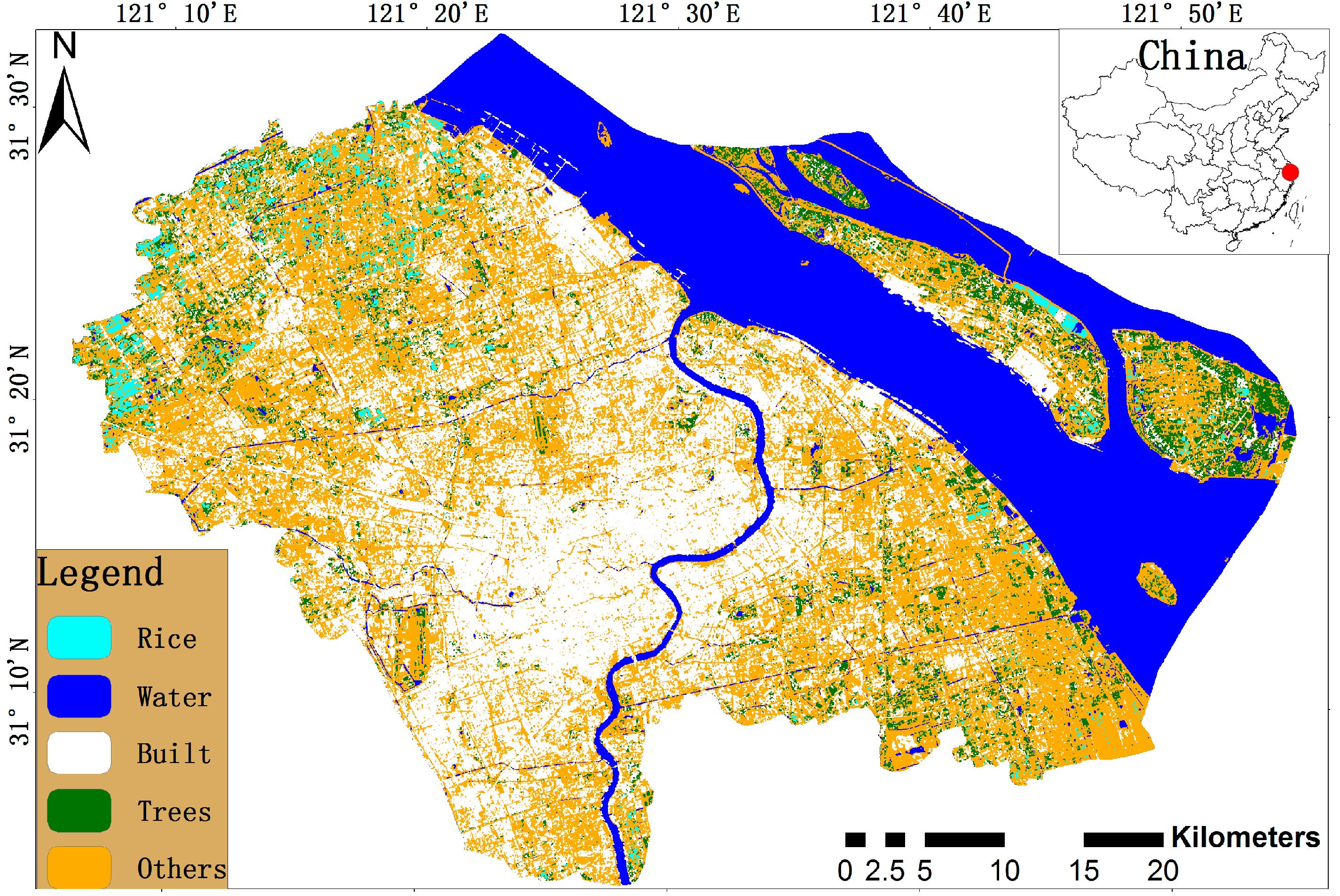
2.1. Study Area

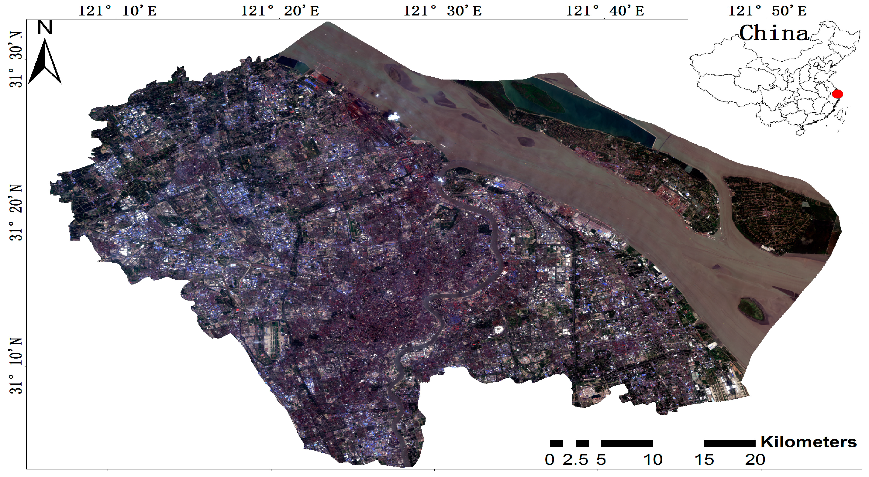
The test site is located in Shanghai, southeast China. It covers the Shanghai central business district (CBD) and its immediate environs. The area under investigation is approximately 2437.7 km², and is centered at longitude 121°5′0.9′′E and latitude 31°8′5.8′′N. It is the most densely populated and most economically intensive part in the Shanghai metropolitan area. The location map of this area is given in Figure 1.

Shanghai is found in the subtropical zone and records annual mean temperatures and rainfall of 15.8 °C and 1149.7 mm, respectively [40]. To support year-round agricultural practices, irrigation schemes are often conducted to supplement insufficient rainfall and meet crop water requirements.

Located in the western North Pacific at the mouth of the Yangtze River, Shanghai is a major commercial hub in China and is home to one of the largest seaports in the world. Shanghai has the highest population density in China, and with its vigorous economic growth, this municipality accounts for about 4.5% of China’s gross domestic product (GDP) [40]. The population of Shanghai continues to soar with increasing migration and arable land for UPA is rapidly becoming scarce.

Several years ago, southeast China including the Shanghai metropolis was one of the major rice producing areas in China. With rapid socio-economic development in this area, more land is required for housing, infrastructure and industry, and rice cultivation is increasingly becoming prominent in northeast China [33]. Even though rice fields have been shifted to the peri-urban, apart from competition from residential and industrial land-uses, they are also seriously contested by such lucrative farming activities as aquaculture, horticulture, and other high income earning and shorter duration crops. Rice fields are therefore becoming smaller and highly fragmented. Much of the paddy rice in Shanghai is now cultivated by subsistence and smallholder commercial farmers. As rice is one major food crop in southeast China, information on its spatial distribution is required for agricultural and food security planning, and in land, water and environmental management.

A single-season rice cultivation system is practiced in Shanghai, which spans from late May to late November. After rice harvest, most of the paddy fields are cultivated with winter wheat, forming the most distinct crop rotation pattern in southeast China. Even though rice is cultivated in a single season in this area, inter-field variability due to different planting dates is evident. Hence, to accurately map rice fields in this area, multi-temporal data are imperative, and the use of multi-source datasets could bring substantial improvements in overall classification accuracies.

2.2. Sentinel-1A Data

Launched in April 2014 by the European Space Agency (ESA) on a SOYUZ rocket from the Guiana Space Center in French Guiana, Sentinel-1A is the first of a series of earth observation satellites for the Copernicus Initiative. The Sentinel-1 mission is the European Radar Observatory for the joint initiative on environment and security between the European Commission and ESA.

The Sentinel-1 synthetic aperture radar (SAR) constellation carries two C-band instruments (1A and 1B) operating at a center frequency of 5.4 GHz, sharing the same orbital plane. Sentinel-1A is a sun-synchronous, near-polar circular orbit at a height of 693 km and an inclination angle of 98.18°. It offers a 12-day repeat cycle at the equator with 175 satellite orbits per cycle. With Sentinel-1A and Sentinel-1B operating, a 6-day repeat cycle at the equator will be achieved [41]. These polar-orbiting satellites acquire images day and night regardless of weather conditions. They continue and compliment C-band imaging missions of ESA’s Earth Resources Satellites (ERS 1 and ERS 2), Environment Satellite (ENVISAT), and Canada’s RADARSAT-1 and RADARSAT-2 [41].

Sentinel-1 presents significant advancement over previous C-band missions as stated above, in terms of spatial and temporal resolution, geographical coverage, reliability and data dissemination [41]. The mission seeks to benefit numerous services as in sea-ice monitoring and maritime surveillance, land monitoring of forest, water, soils and agriculture, monitoring of land surface motions, and mapping to support environment, crisis and natural disaster management [41].

Sentinel-1 operates in four exclusive acquisition modes; Stripmap (SM), Interferometric Wide swath (IW), Extra-Wide swath (EW), and Wave mode (WV). Each mode can produce products at SAR Level-0, Level-1 single look complex (SLC), Level-1 ground range detected (GRD) and Level-2 Ocean (OCN). Level-1 SLC products have been focused and geo-referenced using satellite altitude and orbit data, and are provided in zero-Doppler slant range geometry. Level-1 GRD products are detected, multi-looked and projected to ground range using an Earth ellipsoid model, and phase information is lost. The products have approximately square resolution and pixel spacing with reduced speckle effects at the cost of reduced geometric resolution. GRD products can be in full, high and medium resolution. Level-2 OCN products include Ocean Swell spectra (OSW), Ocean Wind Fields (OWI), and Surface Radial Velocities (RVL). OSW provides an estimate of wind speed and direction per swell spectrum. OWI gives a ground range gridded estimate of surface wind speed and direction at 10 m above the surface. RVL is a ground range gridded difference between the measured Level-2 Doppler grid and the level-1 calculated geometrical Doppler. Of these four acquisition modes of Sentinel-1A, the IW mode is regarded as the primary or default operational mode over land, supporting agriculture, forestry and other natural resource applications [41]. Hence, the IW mode is selected in this study to map rice fields in urban Shanghai.

The IW mode combines a large swath (250 km) with a moderate geometric resolution (5 m by 20 m), and images in three sub-swaths using the Terrain Observation with Progressive Scans SAR (TOPSAR). In addition to steering the beam in range as in SCANSAR, the TOPSAR technique also steers the beam electronically from backward to forward in azimuth direction for each burst, thus, avoiding scalloping and resulting in higher quality images [41]. Interferometry is maintained by the sufficient overlap of the Doppler spectrum (azimuth domain) and the wave number spectrum (elevation domain). TOPSAR ensures homogenous image quality throughout the swath [41].

In this study, we have acquired five Sentinel-1A GRD images in IW mode during the 2015 rice growing season in Shanghai. These images span from the flooding/transplanting stage to the heading/milking stage of paddy rice, a period at which changes in temporal backscatter of the rice crop are most diagnostic. The acquired images are all in dual polarization of vertical transmitted and vertical received (VV), and vertical transmitted and horizontal received (VH) channels. They are in a range and azimuth resolution of 5 m and 20 m, respectively [41]. All images from Sentinel satellite constellations are freely available to consumers and can be downloaded at https://scihub.copernicus.eu/dhus/#/home.

Table 1. Characteristics of Sentinel-1A level 1 GRD IW products used in this study.

Date	AT	RON	PD	ST (GMT)	Polarization	Resolution
9 June 2015	Normal	105	Descending	21:49	VV VH	High
8 July 2015	Normal	171	Ascending	09:54	VV VH	High
1 August 2015	Normal	171	Ascending	09:54	VV VH	High
25 August 2015	Normal	171	Ascending	09:54	VV VH	High
18 September 2015	Normal	171	Ascending	09:54	VV VH	High

AT, RON, PD and ST are acquisition type, relative orbit number, pass direction and sensing time, respectively.

gives a summary of the characteristics of the 5 Sentinel-1A images used in this study. More details on Sentinel-1 products can be found in [41].

2.3. Landsat 8 Data

Landsat provides the longest continuous archive of optical satellite data for land applications. Since its first launch in 1972 with the Multi-spectral Scanner (MSS), Landsat data have significantly improved over the years both in terms of spectral and spatial resolution. The launch of the Landsat 8 Operational Land Imager (OLI) and Thermal Infrared Sensor (TIRS) in February 2013 in particular, has brought new opportunities and a platform for continuity in optical remote sensing. Landsat data are the most widely used in global land-cover mapping and are also freely available to the user community, and can be downloaded at http://glovis.usgs.gov/ or http://earthexplorer.usgs.gov/.

The Landsat 8 carries two instruments: the OLI sensor comprises refined heritage bands from the Enhanced Thematic Mapper plus (ETM+) or Landsat 7, a new deep blue band for coastal/aerosol studies, a shortwave infrared (SWIR) band for cirrus detection, and a quality assessment band. The Thermal Infrared Sensor (TIRS) provides two thermal bands. These sensors onboard Landsat 8, have brought marked improvement in signal-to-noise ratio (SNR) and radiometry is quantized over a 12-bit dynamic range. There are 4096 potential grey levels in Landsat 8 images compared with the 256 in previous 8-bit instruments (Landsat 4, 5 and 7). The improved SNR performance in Landsat 8 enables better land-cover classification, making it suitable for many environmental applications.

Due to persistent cloudy weather conditions in the study area during the rice growing season, only a single cloud-free Landsat 8 image acquired on 3 August 2015 was used in this study. This image is a standard Level-1 terrain corrected (LT1) product on path/row 118/038, projected to the Universal Transverse Mercator (UTM) zone 51 N and World Geodetic System 84 (WGS84) datum.

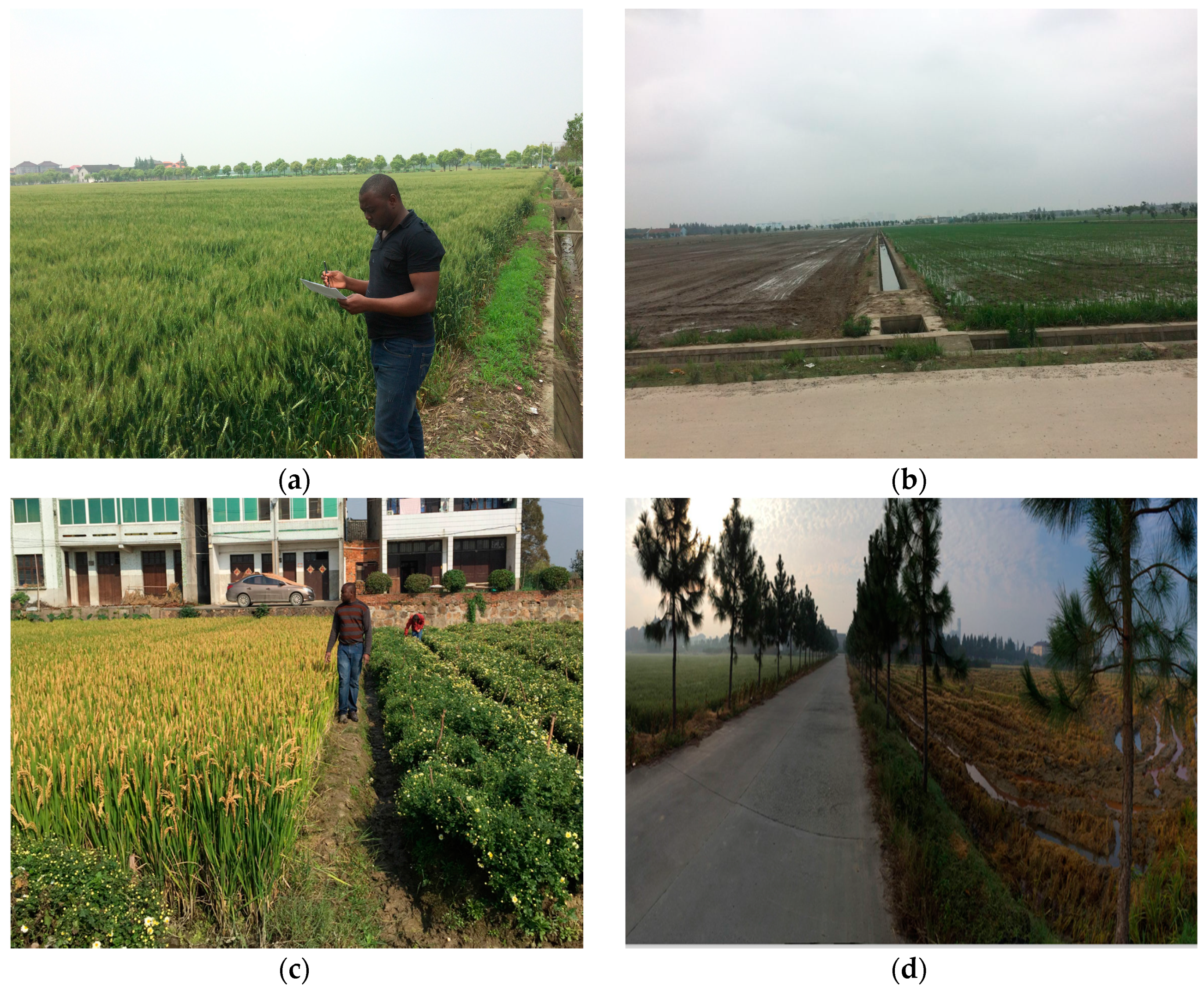
2.4. Field Data

Prior to image classification and accuracy assessment, a field survey of rice fields cultivated in 2015 was conducted from April to May 2016 to obtain training and validation datasets. An ancillary field campaign was also conducted during rice maturity and harvest in November 2016. Rice fields in 2015 were identified through rice stubble (residue), as some of the paddies remained uncultivated after the previous rice harvest. Other 2015 rice fields, which were at the time of our survey cultivated with winter wheat or other crops, were verified through sign boards and interviews with local farmers. Figure 2 shows photos taken during the 2016 field campaigns.

Based on knowledge acquired during the 2016 field campaigns, we have proposed a simplified land-cover classification scheme for the area under study with five broad classes: Rice refers to paddy rice fields; Water includes rivers, lakes, streams and ponds; Built includes residential and industrial estates; Tress include forests and plants with considerable height and density; and Others include transitional areas, paved roads, bare land surfaces, grassland, other low biomass crops, and in the final map could include any or a combination of the other classes due to misclassification. We have adopted this broad classification scheme as the major focus of this study is rice field mapping. The broad land-cover classes of Water, Built, Trees and Others have also been taken into consideration as their coexistence with rice fields could induce confusions and influence Rice classification accuracy.

A total of 150 points, each away from field boundaries, were randomly collected from paddy rice fields using a portable Garmin Global Positioning System (GPS) device, and an average horizontal accuracy of 4.0 m was recorded. From the 150 paddy points, 42 were randomly selected to guide the onscreen digitization of training polygons for the extraction of backscatter coefficients from the temporal Sentinel-1A images. Each of the digitized rice polygons had over 30 pixels. The remaining 108 points were reserved for accuracy assessment. As the other land-cover categories (Water, Built, Trees and Others) are broad and more easily recognizable, 30 training polygons (each over 50 pixels) in each class were directly digitized from high resolution and geo-referenced Google Earth images and exported to Sentinel-1A data for the extraction of temporal backscatter profiles. Additionally, 42 points from Water, and 50 points each from Built, Trees and Others, were randomly selected for the purpose of map accuracy assessment.

Jensen [42] stated that without stratification, it is often difficult to find sufficient samples for classes that occupy a small portion of the study area. Therefore, we have intentionally increased the number of training and validation samples for the Rice class as it forms the major focus of our study. In a highly heterogeneous landscape such as urban Shanghai, accuracy assessment of the rice maps warrants a larger number of samples from the Rice class relative to other land-cover categories. According to [42], the number of samples can also be adjusted based on the relative importance of categories within the objectives of the project or the inherent variability within each category. It may be useful to take fewer samples in categories that show little variability, such as water and forest, and increase the sampling in the categories that are more variable, such as agricultural areas [42]. Hence, though it accounted for the smallest percentage of the scene, we have collected more samples for the Rice class, as it is more variable over time, in addition to being the major focus of our study.

2.5. Image Preprocessing

The five temporal images of Sentinel-1A SAR acquired for this study were automatically preprocessed using the Sentinel Application Platform (SNAP) 2.0 software [43]. SNAP is a common architecture for all Sentinel toolboxes, and is ideal for all earth observation processing and analysis. The images were first calibrated to sigma naught (${\mathsf{\sigma }}^0$) backscatter coefficients using Equation (1). The calibrated images were then automatically terrain corrected using range Doppler terrain correction (producing 10 m square pixel resolution images), reprojected to the Universal Transverse Mercator (UTM) zone 51 N, and speckle filtered using a 7 × 7 gamma map filter with 3 looks [44,45]. Using the 9 June image as master, all the Sentinel-1A images were co-registered on-the-fly in SNAP based on binomial interpolation, using 200 ground control points (GCPs).

$$10 alog10\left(b_0\right)$$

(1)

where $b_0$ is the per pixel signal intensity value or digital number (DN).

The Landsat 8 OLI image used in this study was preprocessed using the Environment for Visualizing Images (ENVI) 5.1 software (ITT Systems, ITT Exelis, Herndon, VA, USA). As optical satellite images are frequently affected by atmospheric effects [46], we employed the darkest object subtraction (DOS) method which has been found most suitable for removing atmospheric effects from cloud-free images [46] as the one used herein. The atmospherically corrected Landsat 8 image was subset to the areal extent of the test site. This image subset was geometrically corrected using 30 GCPs located at major intersections or easily identifiable features across the study area, and a root mean square error (RMSE) of less than 0.5 pixel (<15 m) was recorded. A 4-band spectral subset comprising the green (0.53–0.59), red (0.64–0.67), NIR (0.85–0.88) and SWIR 1 (1.57–1.65) bands was then generated. These 4 multispectral bands were selected for the derivation of optical indices that will be combined with the temporal Sentinel-1A data for the land-cover mapping in this study.

The final preprocessing involved a PAN-sharpening of the 30 m Landsat OLI image (selected 4 bands) to the 10 m square pixel resolution of Sentinel-1A. PAN-sharpening involves the merging of a panchromatic image (PAN) with a multispectral image (MSI) inorder to increase the spatial resolution of the latter, while simultaneously preserving its spectral information [47]. In this study, both datasets (Sentinel-1A as PAN and Landsat 8 as MSI) have been geo-referenced and projected to the same cartographic plane (UTM 51 N, WGS 84). The Gram-Schmidt Spectral Sharpening method was used to sharpen the multispectral Landsat data with the higher resolution Sentinel-1A data. Gram-Schmidt is an effective multispectral image sharpening method as it uses the spectral response function of a given sensor to estimate what the panchromatic data look like. It has been recommended for most remote sensing applications [47,48] and is therefore, utilized in this study.

2.6. Image Classification

A decision tree classification algorithm is implemented in this study based on the spatial and temporal distribution of backscatter coefficients obtained from Sentinel-1A data and optical indices derived from the single Landsat image. A decision tree classifier is independent of data probability distributions [23]. It employs tree-structured rules which recursively divide the initial input dataset into increasingly homogeneous subsets based on well defined splitting criteria [49]. At each split or node, the values of each explanatory variable are examined and a particular threshold of a single variable that produces the largest reduction in a deviance measure is chosen to partition the data [50]. Decision tree classifiers are advantageous in that they are less sensitive to nonlinearities in the input data than classification methods that require an assumption of Gaussian distributions [50,51].

As the Sentinel-1A data used in this study are in dual polarization of VV and VH, we have attempted to propose the most optimal polarization for mapping the targeted land-cover types. We have decided to use a single polarization in order to reduce data redundancy and dimensionality, as Landsat 8 optical indices are also utilized. In [52], similar to using multiple or dual polarization data, a corresponding increase in accuracy is expected when the inputs to the classification algorithm consist of measurements acquired at different dates.

Two criteria were considered in the selection of the optimal polarization. The first criterion is based on the temporal increase of paddy rice backscatter, whereas the second exploits a two-class separability measure. The optimal polarization is assumed to be the one which exhibits the most sustained increase in paddy rice backscatter, while at the same time producing the best results with the two-class separability measure. In other words, a polarization has to satisfy both conditions to be considered optimal or else both polarizations will be used as inputs in the decision tree classifier.

According to the concept of feature separability [53], two classes are said to be well separated if the distance between their respective class means is larger than that of their standard deviations. The separability criteria between classes a and b is measured by the Bahattacharrya distance [54] as:

$$S_{ab}=\frac{\left|{\mu }_a-{\mu }_b\right|}{s_a+s_b}$$

(2)

where μ and s are the mean and standard deviation of the features to be separated, respectively. The Bahattachayrrya distance is theoretically sound as it is directly related to the upper bound of classification error probabilities [23]. It measures the real values between 0 and 2, where 0 indicates a complete overlap between two classes, and 2 indicates a complete separation between them [55]. The larger the separability values among class pairs, the better the final classification results [23,49].

The normalized difference vegetation index (NDVI) and the normalized difference water index (NDWI) were the two optical indices generated from the PAN-sharpened (10 m) Landsat 8 image for combination with the temporal Sentinel-1A data. NDVI has been widely applied in monitoring various vegetation cover, and is frequently used as a proxy of plant growth and productivity, as the amount of solar radiation reflected by the vegetation canopy is related to wavelength, chlorophyll, leaf interior tissues and plant water content [56]. NDWI is as important to the monitoring of water bodies as NDVI is to the monitoring of vegetation canopies. In this study, we have employed the modified NDWI (MNDWI) proposed by [57] which cannot only enhance information about water and restricting the one from vegetation and soil, but can also significantly distinguish built-up features from water bodies. These optical indices have been derived using the following equations:

$$NDVI=\frac{b_{nir}-b_{red}}{b_{nir}+b_{red}}$$

(3)

where $b_{nir}$ is the near infrared band and $b_{red}$ is the red band.

$$MNDWI=\frac{b_{green}-b_{swir}}{b_{green}+b_{swir}}$$

(4)

where $b_{green}$ and $b_{swir}$ are the green and shortwave infrared bands, respectively.

Land-cover classification accuracies have been improved with the conjugative use of optical and microwave datasets [39,43]. In the current study, it is proposed that the integration of the aforementioned optical indices with temporal microwave data could provide additional information that would improve overall classification accuracy. The 5 Sentinel-1A images from the optimal polarization and the NDVI and MNDWI images were finally layer stacked via bilinear interpolation to produce a 7-band dataset as follows: 9 June image (b1), 8 July Image (b2), 1 August image (b3), 25 August image (b4), 18 September image (b5), 3 August NDVI image (b6) and 3 August MNDWI image (b7).

The collected training polygons as stated in Section 2.4 were used to extract backscatter profiles of the targeted land-cover categories using the optimal polarization. Average backscatter values in decibels (dB) were calculated for each training polygon in each class. Then the average temporal backscatter profile was calculated for each land-cover class. Based on the temporal backscatter of the investigated land-cover classes at the optimal polarization and the spatial distribution of NDVI and MNDWI values, a decision rule mapping algorithm is proposed and validated in this study.

2.7. Mapping Algorithm

In our proposed algorithm, we have made an initial categorization of the Rice class into two subclasses (A and B) so as to take into account the different planting dates which cause differences in growth stages and hence temporal backscatter between rice fields. Such variations could trigger omissions in the Rice class. In the final map however, the Rice subclasses have been merged into a single Rice class. Our proposed mapping algorithm is described along the following paragraphs.

A hierarchical knowledge-based decision rule classier has been employed in this study. As stated in [23,47,58], this knowledge can be heuristic, i.e., based on experience and reasoning. We have developed the classification rules based on our expert knowledge of class signatures and data characteristics using the per pixel information in each image, with its temporal behavior, and the corresponding temporal backscatter coefficients (dynamic range, minimum and maximum) and the single-date optical indices in each of the land-cover types. Dynamic and variable thresholds have been employed to discriminate paddy rice fields from the other land-cover. All 7 images in the co-registered layer stack described in Section 2.6 are used as input datasets in the decision tree.

For the identification of Rice, the observed dynamic range of backscatter values in this class is from −23.5 to −13.5. As the Rice class showed the most dynamic backscatter range among the classes investigated and being that there is wide inter-field variability in planting dates and hence growth conditions, we have proposed two temporal thresholds for Rice discrimination. Firstly, all pixels less than or equal to −19.0 dB and greater than or equal to −17.0 dB from b1 (9 June) to b2 (8 July) or from b1 to b3 (1 August), or from b2 to b3, and with b6 (NDVI) greater than or equal to 0.3 but less than 0.5 are classified as Rice. Secondly, all pixels less than or equal to −18.0 dB and greater than or equal to −16.0 dB from b1 to b2 or from b1 to b3, or from b2 to b3, with b6 greater than or equal to 0.3 but less than 0.5 are classified as Rice. NDVI is derived from a 3 August image. From field information, late planting of paddy rice in this area in 2015 was done within the first week of July. In view of the observed paddy rice phenology in this area, at 3 August, even late planted rice is already 3−4 weeks old, corresponding to a part of the vegetative stage, in which NDVI values are no less than 0.3 [59]. These rules are expected to reduce, if not eliminate confusions involving Rice.

For the identification of Water, the maximum backscatter value of water or flooded surfaces is below −18.0 dB. Therefore, all pixels for which after the extraction of Rice were less than −18.0 dB at any three consecutive dates of imaging (b1−b3, b2–b4, or b3–b5), and with a positive MNDWI and negative NDVI are classified as Water. Between subsequent dates of SAR imaging, a backscatter increase could be recorded over a water surface due to an increase in surface roughness caused by moving elements such as winds or boats as is mostly common along rivers and coastlines. The introduction of a consecutive three-date temporal backscatter below −18.0 dB could offset the effect of isolated increases in backscatter between dates of SAR imaging. Additionally, the use of optical indices could eliminate the influence of any spontaneous increase in temporal backscatter.

For the mapping of Built, all pixels greater than −13.0 dB at any three consecutive dates of imaging (b1–b3, b2–b4, or b3–b5), and with a negative NDVI were classified into this category. This class exhibited the highest temporal backscatter values due primarily to corner reflections from buildings and other vertical objects [45]. As we have placed other low backscatter surfaces such as asphalt pavements into the class “Others” and as the temporal backscatter profile of Built is far removed from that of Water, the MNDWI image was not applied in the mapping of Built.

For the mapping of Trees, all pixels for which after the extraction of Built were greater than −16.0 dB at three consecutive dates of imaging as stated above, and with b6 greater than or equal to 0.5 were put into this category. Trees exhibited the second highest backscatter, and as its temporal backscatter profile is also far away from that of Water, there was no need to utilize the MNDWI.

Finally, all pixels which do not meet the classification criteria outlined above, were classified as Others, a class which as earlier mentioned, contains roads, barren, grasslands and other low biomass plants, and in the final land-cover map, could include misclassified pixels from Rice, Water, Built and Trees. Results obtained from this algorithm were validated via accuracy tests.

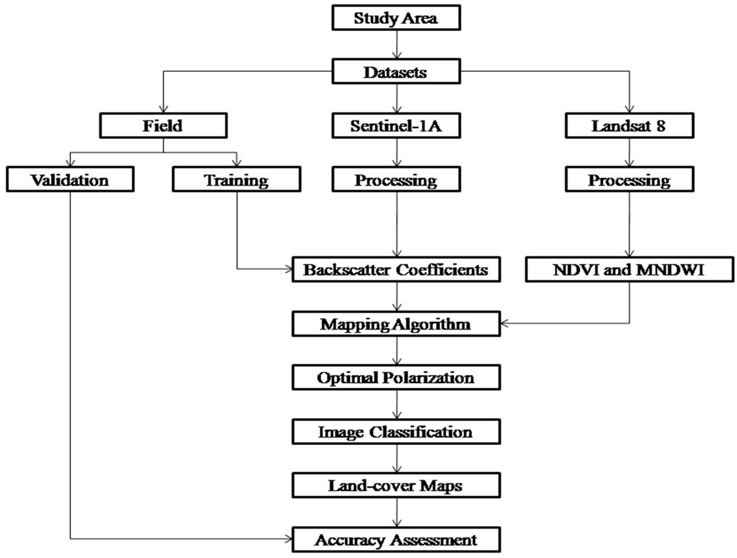
2.8. Accuracy Assessment

As stated in Section 2.4, 108 Rice points obtained from the 2016 field survey, 42 Water points and 50 points from each of the other land-cover types, derived from geo-referenced and high resolution Google Earth images, were used in a post-classification accuracy assessment. An error/confusion matrix was generated, and from which the producer’s accuracy, user’s accuracy, Kappa (statistic) index of agreement and overall classification accuracy of our mapping algorithm were calculated.

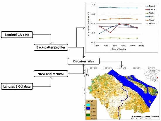
The methodological approach adopted in this study is illustrated in the flow chart below (Figure 3).

3. Results

3.1. Optimal Polarization Images

In determining the optimal polarization based on the temporal increase in paddy rice backscatter, backscatter profiles of training polygons were critically examined at both VV and VH polarizations. It is observed at these two polarizations that at the start of the growing season, out of the 42 paddy rice training polygons, 14 showed lowest backscatter at the first available image (9 June/b1), while the remaining 28 showed lowest backscatter at the second available image (8 July/b2). In any paddy rice field, lowest backscatter values are recorded at the flooding and planting stages. Hence, we first made a temporal distinction of paddy rice fields based on the apparent time of lowest backscatter as follows: Rice A as fields whose lowest backscatter at the start of the season were recorded by the 9 June image; Rice B as fields whose lowest backscatter at the start of the season were recorded by the 8 July image. In effect, Rice A are fields planted before 9 June, and Rice B are those planted after 9 June.

Table 2. Temporal backscatter coefficients for all land-cover classes at VH polarization.

	Rice A		Rice B		Water		Built		Trees		Others
Image	μ	s	μ	s	μ	s	μ	s	μ	s	μ	s
9 June	−20.2	1.0	−17.2	1.9	−22.3	3.1	−9.2	4.2	−14.4	0.6	−17.2	2.1
8 July	−17.7	1.3	−19.7	1.0	−22.0	2.1	−9.0	4.3	−14.0	1.0	−17.1	2.2
1 August	−16.3	0.7	−16.2	0.9	−22.1	2.4	−9.3	4.3	−13.9	1.0	−17.5	1.6
25 August	−16.9	0.9	−16.4	0.8	−22.2	2.2	−9.4	4.3	−13.8	0.9	−17.7	2.2
18 September	−17.7	1.0	−17.8	1.1	−22.1	2.4	−9.2	4.3	−14.1	0.6	−17.4	1.9

μ and s are the mean and standard deviation, respectively, of backscatter (dB) at corresponding class and date.

and

Table 3. Temporal backscatter coefficients for all land-cover classes at VV polarization.

	Rice A		Rice B		Water		Built		Trees		Others
Image	μ	s	μ	s	μ	s	μ	s	μ	s	μ	s
9 June	−12.6	2.0	−9.8	2.4	−15.4	2.9	−0.9	3.6	−7.5	0.6	−10.7	3.7
8 July	−8.3	1.5	−11.0	2.0	−14.4	2.6	−2.0	3.2	−7.0	1.0	−9.9	4.1
1 August	−9.7	1.7	−9.3	1.7	−13.7	1.9	−2.5	3.2	−7.3	1.1	−10.4	3.5
25 August	−10.9	1.5	−10.2	2.2	−15.3	2.0	−2.2	3.2	−7.0	0.8	−10.2	4.0
18 September	−12.5	2.0	−13.4	1.8	−14.8	2.6	−2.3	3.2	−7.6	0.9	−10.4	3.9

μ and s are the mean and standard deviation, respectively, of backscatter (dB) at corresponding class and date.

show the extracted average temporal radar backscatter coefficients and their corresponding standard deviations at VH and VV polarizations for the two Rice subclasses and the broad land-cover categories of Water, Built, Trees and Others.

Figure 4 shows the average temporal backscatter profiles of Rice at both VV and VH polarizations. It can be observed from Figure 4 that the temporal backscatter at the VV channel is higher than that at VH at all imaging dates, in agreement with results obtained in [38,45]. However, the VH polarization indicates the most consistent temporal increase in paddy rice backscatter. The consistency is here defined as the number of time points at which an increase in backscatter is recorded. For Rice A, there is an increase in backscatter up to the third image date (1 August 2015) at VH polarization, as opposed to a VV polarization in which the increase stopped at the second image date (8 July 2015). For Rice B, even though the increase in backscatter saturates at the second image for both polarizations, the VH channel shows a relatively shallow decline compared to the steep decline at VV. As stated in [38], the physical basis for the more sustained increase in rice temporal backscatter at VH polarization is attributable to the VH signal being less affected by changes in surface water and therefore could better reveal rice growth conditions. Furthermore, Le Toan et al. [60] attributed this to the stronger attenuation of vertical cylinders (leaves and stems) at the VV than at the VH channel. These backscatter dynamics have also been observed in [23], and, hence, substantiate our results. We have therefore, supposed the VH polarization to provide a better discrimination of Rice from other land-cover categories whose temporal backscatter profiles are generally stable during the paddy rice growing season in the area under investigation.

Results on the determination of the optimal polarization channel based on two-class signature separability measures are given in

Table 4. Comparison of two-class separability results at VH and VV polarizations.

Class Pairs	VH Polarization	VV Polarization
Rice and Water *	1.1	1.0
Rice and Built	1.6	1.6
Rice and Trees *	1.9	1.0
Rice and Others *	0.4	0.1
Water and Built **	1.9	2.2
Water and Trees *	2.3	2.1
Water and Others *	1.1	0.7
Built and Trees **	0.9	1.3
Built and Others *	1.3	1.2
Trees and Others *	1.1	0.6

* Class pair in which VH has better separability than VV, and ** class pair in which VV separates better than VH.

. Results are computed using Equation (2) in Section 2.6.

From Table 4, the class pair “Rice and Others” is not linearly separable as the latter is a combination of surface features (bare soils, asphalt pavements and grassland) which generally exhibit similar (low) backscatter values especially at the start of the rice growing season. However, as our mapping strategy is based on multi-temporal data, these classes can be separated based on the increase in temporal backscatter of rice at the start of the growing season, as opposed to the relatively linear backscatter profile of “Others” at periods corresponding to the rice growing season.

In general, a separability value below 0.8 is regarded not large enough to separate two classes. Between 0.8 and 1.5, the quality of the separation between the two classes is regarded as average. Values above 2.0 indicate almost complete separability between classes [53,54]. From Table 4, it can be observed that with exception of the class pairs “Water and Built” and “Built and Trees”, the VH polarization produces better inter-class signature separability.

Based on the most sustained increase in paddy rice backscatter at the VH polarization, and the superiority of the VH over the VV channel in the two-class separability measure, we have, therefore, proposed the VH polarization as the optimal polarization and with which the optical indices are combined for the mapping of rice fields and the other land-cover categories in this study. It has also been observed in [52] that at C-band, cross (VH) polarization produces better crop classification results than the like (VV) polarization, and that the use of dual polarization does not further improve the classification results. Figure 5 shows the temporal backscatter profiles of the two Rice subclasses (Rice A and Rice A) and the other broad land-cover categories at the VH polarization.

In Figure 5, it can be clearly seen that, apart from the two Rice subclasses, the other land-cover classes show linear temporal backscatter profiles during the paddy rice growing season. Therefore, based on the observed increase in the backscatter of paddy rice at the first two months of growth and its steady decline thereafter relative to the almost stable temporal backscatter profiles of the other land-cover classes, and the spatial distribution of single-date NDVI and MNDWI values, we have presented results from two mapping algorithms; one obtained only from the temporal VH images of Sentinel-1A and the other derived from the synergistic application of temporal Sentinel-1A images and single-date Landsat indices. The latter algorithm (described in Section 2.7) is, however, proposed in this study as it produced much better classification accuracy.

3.2. Mapping Results from Sentinel-1A

Results from the use of only the temporal VH images of Sentinel-1A are presented in Figure 6.

In Figure 6, it can be observed that there are wide misclassifications especially with Rice, Water and Trees. Some pixels within deep water surfaces have been classified as Rice. Even on land, certain pixels have been misclassified as Rice, such as in lawns and asphalt pavements. These areas typically show low microwave backscatter. As the prevalence of surface winds could increase the roughness and, hence, the backscatter signals at a subsequent acquisition, some of these pixels could be misclassified as Rice. Water pixels can also be found in dryland surfaces such as asphalt pavements and lawns. Additionally, in a highly urbanized landscape such as Shanghai, it is very unlikely to find such a large area covered by trees, as can be observed in Figure 6. The class “Trees” has virtually taken all the areas that are likely to be occupied by the class “Others” (as defined in this study). The accuracy assessment report for the land-cover map presented in Figure 6 is given in

Table 5. Error matrix of accuracy assessment of classification with Sentinel-1A VH images.

Classes	Rice	Water	Built	Trees	Others	Row Total
Rice	107	3	2	1	6	119
Water	1	38	2	1	7	49
Built	0	0	44	2	7	53
Trees	0	0	2	38	18	58
Others	0	1	0	8	12	21
CT	108	42	50	50	50	300
PA (%)	99.1	90.5	88.0	76.0	24.0
UA (%)	89.9	77.6	83.0	65.5	57.1
Overall Classification Accuracy: 79.7%				Kappa Statistic: 0.73

CT, PA and UA are column total, producer’s accuracy and user’s accuracy, respectively.

.

In Table 5, even though almost all validation points of Rice have been correctly classified, there are some commission errors in this class. Much of the commission errors in Water are derived from the misclassification of Rice. In addition, much of the omission errors in the class “Others” are derived from the misclassification of Trees. Built shows a relatively good agreement with ground reference data.

3.3. Mapping Results from Sentinel-1A and Landsat 8

Results from the proposed mapping algorithm, which utilizes both the temporal VH images of Sentinel-1A and the single-date NDVI and MNDWI from Landsat 8 are presented in Figure 7.

In Figure 7, the wide classification errors observed in Figure 6 have been reduced significantly with the introduction of single-date optical indices (NDVI and MNDWI). The map shows greater class homogeneity as much of the misclassified, island or mixed pixels have been eliminated. Rice and Water are more clearly delineated. Rice pixels can now only be seen inland, and in places where rice cultivation is most likely. The area covered by Trees has significantly reduced as a consequence of the increase in the area covered by the class “Others”. Additionally, some of the pixels (bare surfaces, asphalt pavements, grassland, etc.) initially misclassified as Water have now been categorized into the class ”Others”. The Built category still maintains its relatively good agreement with reference data. The class accuracy assessment report of Figure 7 is given in

Table 6. Error matrix of accuracy assessment of classification with Sentinel-1A VH and Landsat 8 OLI.

Classes	Rice	Water	Built	Trees	Others	Row Total
Rice	104	0	0	0	0	104
Water	2	39	1	0	0	42
Built	0	0	43	2	7	52
Trees	0	0	0	31	5	36
Others	2	3	6	17	38	66
CT	108	42	50	50	50	300
PA (%)	96.3	92.9	86.0	62.0	76.0
UA (%)	100	92.9	82.7	86.1	57.6
Overall Classification Accuracy: 85.0%				Kappa Statistic: 0.81

CT, PA and UA are column total, producer’s accuracy and user’s accuracy, respectively.

.

In Table 6, the commission errors previously recorded in Rice have all been eliminated, with however, a few omission errors. There is a slight decrease in the accuracy of Built, but that of Water increases. The improvement in the UA of Trees corresponds to the improvement in the PA of Others.

In Figure 6 and Figure 7, it can be clearly seen that, excluding the apparent commission errors in the Rice class in Figure 6, there seems a perfect agreement on the spatial distribution of rice fields between the two maps. Paddy rice cultivation is mostly concentrated in the northeastern part of the study area, which mainly includes the urban Shanghai districts of Jiading and Baoshan.

4. Discussion

Sentinel-1A offers a new opportunity for environmental monitoring at finer spatio-temporal scales. These data have already been tested in rice and land-cover monitoring [38,39,43]. However, specific applications of these data in mapping subsistence or smallholder commercial rice agriculture typical in urban landscapes are yet to be undertaken. In this study, we have combined these new SAR data with the Landsat 8 OLI data to map rice fields in urban Shanghai, southeast China, during the 2015 growing season.

Even though a single-season rice cultivation system is practiced in the study area, there is still wide inter-field variability in the growth of rice crops, due mainly to differences in planting dates and varieties. As temporal backscatter coefficients of rice are largely a function of rice growth stage and conditions, inter-field differences could affect the performance of rice mapping algorithms in which temporal backscatter change is used as the main classification feature. In a single-season rice cultivation system, planting dates could vary up to eight weeks between adjacent paddy rice fields [24]. Additionally, differences in variety and management practices could lead to marked differences in growth conditions, and, hence, temporal backscatter. Therefore, using the temporal backscatter change as a classification feature, a major source of uncertainty could arise due to different radar response patterns between fields. This calls for the application of a high temporal frequency of SAR observations that would capture even subtle differences in backscatter values between rice fields.

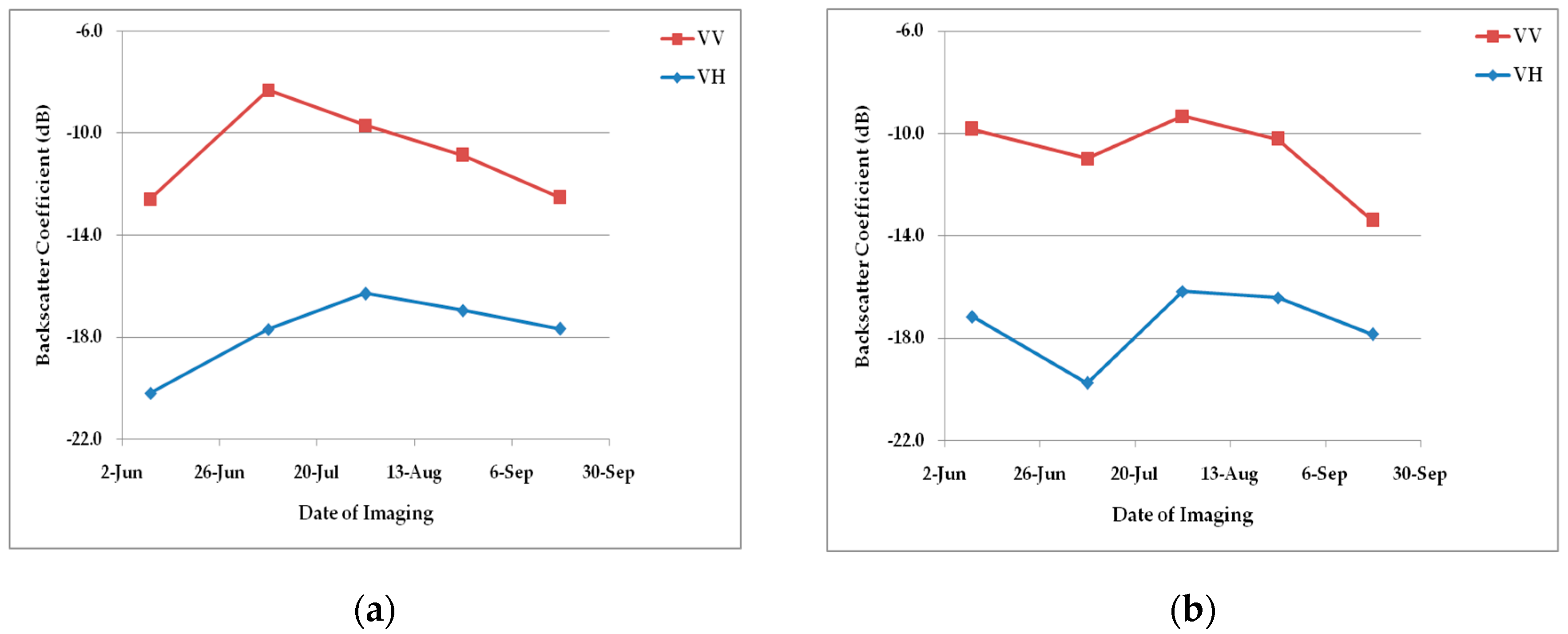
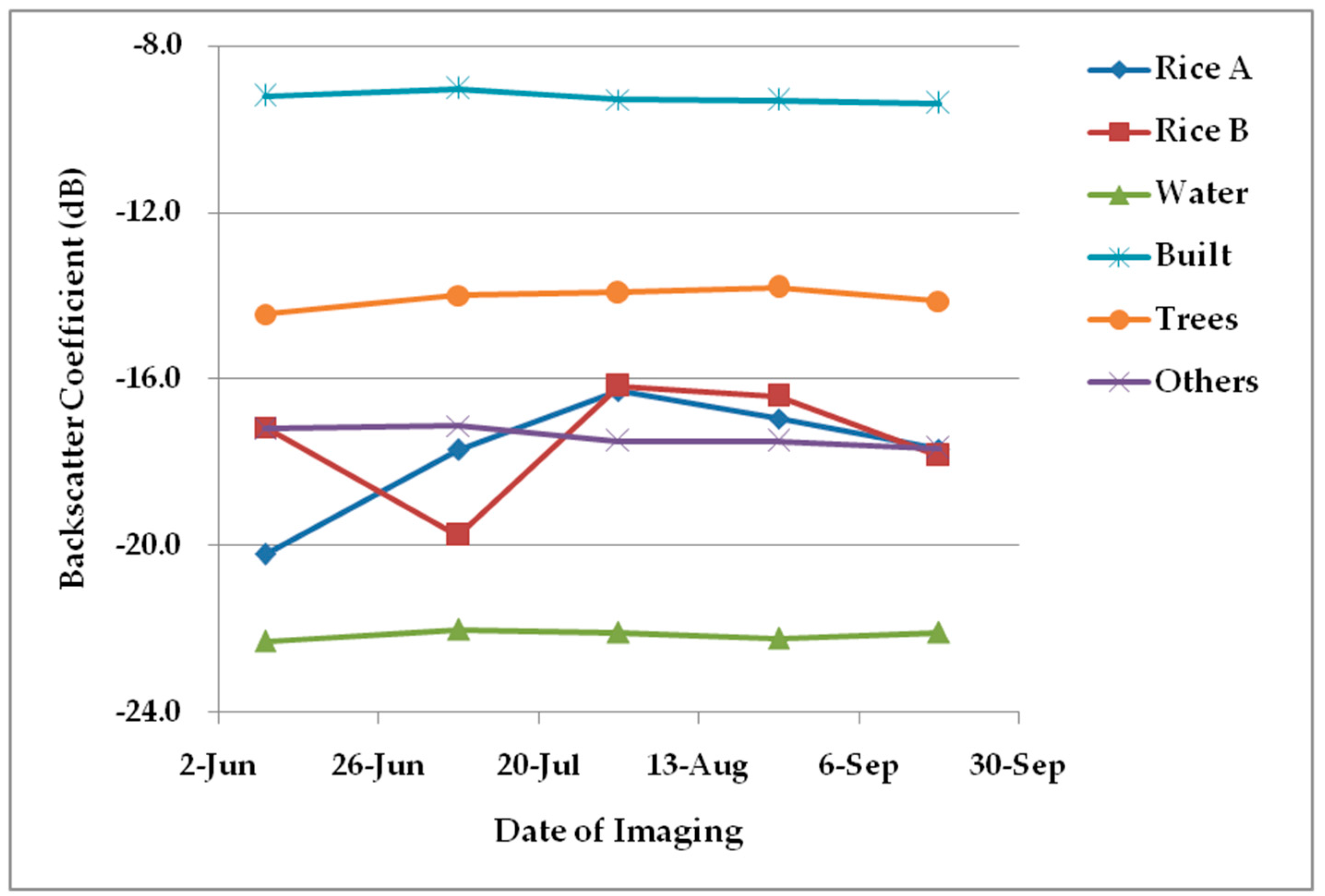
In this study, we have employed five temporal images of Sentinel-1A, covering a part of the rice growing season (planting to heading) in which changes in backscatter values are most pronounced. From an analysis of the temporal backscatter of paddy rice, we confirmed the variations in planting dates based on the time of lowest backscatter at the start of the growing season. The time of lowest backscatter for paddy rice at the start of the growing season is at flooding and planting. We have therefore, initially categorized the Rice class into two: Rice A, are those fields in which the lowest backscatter at the start of the season is recorded by the 9 June image; Rice B, are those in which the lowest backscatter at the start of the season is recorded by the 8 July image. Out of the 42 Rice training samples, none recorded lowest backscatter in the 1 August image, implying that, in 2015, planting was conducted from early June to early July for most, if not all, the rice fields in the study area.

It is observed in this study that the temporal backscatter profiles at the VV polarization are higher for all land-cover classes, which is in agreement with results obtained in [45]. However, the VH polarization exhibited the most sustained increase in backscatter of Rice A, increasing sharply from flooding/planting to apparent tillering and booting, and decreasing slightly at heading. With the VV channel, the temporal increase in backscatter saturates at the second available image for both Rice subclasses (A and B). For Rice B, even though the increase in backscatter saturates at the second image for both polarizations, the VH channel shows a relatively shallow decline compared to the steep decline at VV polarization. Using two-class separability measures reported in [51], the VH polarization is also found to have an overall better performance in discriminating the investigated land-cover classes. Hence, given its more sustained increase in temporal backscatter with rice and its better inter-class signature separability, the VH polarization was regarded optimal for our study, and whose temporal images were used in subsequent analysis.

As would be expected, Water showed the lowest temporal backscatter, a feature attributable to the smooth or specular reflections from the water surface [23]. Built exhibited the highest temporal backscatter profile, which is largely ascribed to corner reflections from buildings and other vertical objects [49]. Trees also showed a high temporal backscatter profile second only to Built. Excluding the Rice subclasses, the class “Others”, which comprises bare soils, paved roads, herbaceous cover, grass and other low biomass crops, showed a temporal backscatter profile higher only than that of Water. This is due to the significant influence of roads in the class “Others”. Even in optical images, asphalt materials could show low reflectance. From a visual inspection of the individual pixels of highways and airport runways, we observed a low temporal backscatter closer to the maximum backscatter value recorded at the flooding stage of rice. The temporal backscatter profile of the class ”Others” is approximately mid-way between the peaks and troughs of rice temporal backscatter.

As stated earlier, the first mapping results presented in this study are only based on five VH images from Sentinel-1A. We have employed as a classification feature, the temporal increase in rice backscatter during the first two months of growth, and its steady decline thereafter relative to the nearly uniform temporal backscatter profiles of the other land-cover classes. The resultant land-cover map from this approach shows serious misclassifications of Rice, Water, Trees and Others. Even though almost all validation Rice pixels were correctly classified, there were some commission errors in this class. Several Water pixels have been misclassified as Rice. This is one major source of uncertainty in paddy rice mapping algorithms solely based on the temporal increase in backscatter. It is important to note that an increase in surface roughness, which could be induced by moving objects such as wind or boats, could increase the backscatter value of a given pixel between SAR acquisitions [28]. If this backscatter increase is within the observed dynamic range of paddy rice backscatter and also fall within the lower and upper limit thresholds, such a pixel will be categorized as Rice. Several confusions also exist between Trees and Others, and between Water and Others. Figure 6 shows a relatively large area covered by Trees, a condition that is very unlikely in this area. Much of the pixels of the class “Others”, especially those of herbaceous plants, have been misclassified as Trees. Several pixels of the class “Others” have equally been misclassified as Water due to significantly low backscatter profiles of areas covered by grass and asphalts pavements. In order to eliminate some of these confusions, we have combined the temporal VH images with the NDVI and MNDWI images.

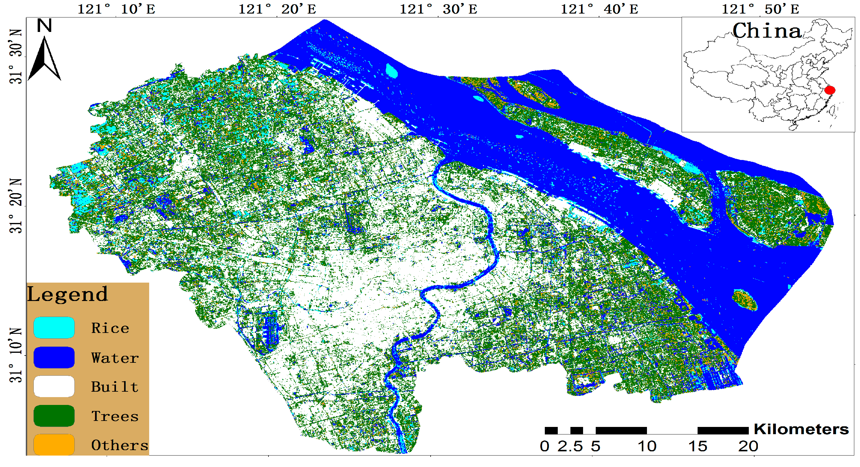
The introduction of the aforementioned optical indices into our mapping algorithm brought a significant reduction in inter-class confusions as evident in the respective producer’s and user’s accuracies. In the Rice class, these optical indices eliminated all the commission errors derived from omissions in the other classes. Our study area is not only located along the coast but is also home to large rivers including the famous Huangpu River. As boats and other marine vessels frequently sail along these waterways, the backscatter of a given pixel could increase between dates of imaging. Furthermore, this area is prone to subtropical monsoon winds, which occur during the rice growing season. Thus, sporadic or spontaneous increases in surface roughness and, hence, SAR backscatter are most likely, which could lead to misclassification of Water pixels as Rice. Water and Built typically have negative NDVI values, and therefore, the introduction of this optical index removed all Water and Built pixels misclassified as Rice on the basis of a temporal increase in backscatter. In Table 5, half of the commission errors in the Rice class are accounted for by the class “Others”. With the introduction of the condition, 0.5 > NDVI ≥ 0.3, all commission errors in the Rice class derived from omissions in “Trees and Others” were eliminated. It is assumed that at 3 August (date of optical indices), rice plants in the study area would have acquired enough surface area for NDVI to be greater than or equal to 0.3, but less than 0.5. The use of the condition, NDVI ≥ 0.5, significantly reduced the commission errors in Trees, thereby increasing the PA of Others, and hence, an overall increase in the classification accuracy of Trees and Others. It can be observed that most of the areas initially misclassified as Trees in Figure 6 have been classified as “Others” in Figure 7. This is quite agreeable with ground reference data as the class “Others” occupies a larger portion in the study area.

As the major focus of this study is urban rice mapping, it is extremely important to note the comparative advantages of the two mapping algorithms in discriminating rice fields. With the incorporation of optical indices, there is a slight decrease in the PA of Rice but a substantial increase in its UA. The slight decrease in the former is attributable to the omission errors associated with the use of NDVI. We have proposed that a pixel is classified as Rice when it meets the temporal backscatter change criterion, while having NDVI values ≥ 0.3 but < 0.5. The three additional pixels eliminated from the Rice class with the introduction of NDVI is likely due to the fact that, even within a plot of rice, growth is not uniform, and pixels which may fall below a critical threshold could be removed from the Rice class. With the sole use of the temporal VH images, only one Rice validation point was eliminated. However, results obtained from the sole use of VH images are largely misleading due to the commission errors in the Rice class, and of course also, the commission errors in Water, Built and Trees, which are as a result of the large omission errors in the class “Others”. With the integration of the temporal VH images of Sentinel-1A with the single-date Landsat 8 OLI’s NDVI and MNDWI images, there is a substantial increase in the class accuracy of Rice and the reduction of commission and omission errors in the other classes brought a slight increase in overall classification accuracy.

5. Conclusions

Globally, little research effort has been directed towards urban agricultural mapping, where land dedicated to rice cultivation in particular, is increasingly becoming smaller and fragmented by other land-uses. With rice production forming an integral part in meeting global food demands, it is important to not only monitor rice cultivation at large scales, but also those at relatively smaller scales such as in urban areas. Furthermore, rice cultivation is at the center stage of global environmental debates involving greenhouse gas emissions and water resource allocation. However, the contribution of urban rice agriculture to the above environmental issues is largely ignored due to limited urban agricultural information. In an attempt to fill some of the knowledge gaps in agricultural mapping in urban landscapes, this study is conducted to test the potential of integrating the new Sentinel-1A SAR data with Landsat 8 optical data for urban rice mapping.

In this study, we have noted the VH polarization of Sentinel-1A to be the optimal polarization for rice field mapping as it exhibited the most sustained increase in the temporal backscatter of rice, relative to the nearly uniform temporal backscatter profiles of the other land-cover classes. Using a two-class separability measure, the VH polarization showed better inter-class discrimination ability, and was thus combined with NDVI and MNDWI images in our proposed rice mapping algorithm.

With the introduction of NDVI and MNDWI, overall classification accuracy increased from 79.7% to 85.0%, and the Kappa statistic from 0.73 to 0.81. The slight increase in overall classification accuracy (5.3%) has demonstrated the added value of limited optical data to the more available radar data in cloud-prone tropics and subtropics for land-cover mapping. We strongly suppose that with more temporal optical data, the potential of SAR data in paddy rice mapping will be fully realized. The increase in Rice user’s accuracy (reduction in commission errors) with the addition of these two optical indices confirms the operational applicability of integrating the new Sentinel-1A data with optical data for rice mapping in subtropical and highly heterogeneous landscapes.

It can be observed in Figure 7 that the rice parcels are located in the peripheral areas of the study site. This indicates the gradual shift of rice cultivation to the urban fringe and peri-urban as a consequence of urban expansion and industrialization. Additionally, the intensification of urban agricultural land-uses such as vegetable gardening, fruit farming and aquaculture has reduced the amount of land allocated to rice cultivation. Apart from providing better rents than rice, perishable goods such as vegetables, fruits and fish require closer proximity to urban markets and consumers. Hence, rice fields are increasingly becoming smaller and fragmented by other agricultural land-uses in urban areas such as Shanghai. However, rice being a major staple food means its cultivation is still central in the attainment of global food security and in urban areas could not only meet food demands at household levels but also provide an alternative employment for unskilled or urban surplus labor. Even though our study has only mapped rice fields at a single time point (2015), our results could be instrumental in updating previous records while providing a basis for revealing the spatio-temporal dynamics of rice cultivation in urban Shanghai and its potential impacts on food availability, greenhouse gas emissions, water resource utilization and land-use management. This study could be regarded as one of, if not the first, to test the operational applicability of integrating the new Sentinel-1A data with Landsat 8 data for mapping smallholder rice fields in an urban landscape at a district scale, providing details of individual rice field boundaries. Moreover, our study, having shown the VH polarization to increase sharply after planting and decrease steadily at heading, demonstrates the potential of Sentinel-1A in monitoring other rice biophysical parameters that show similar temporal behaviors such as above ground biomass and leaf area index. Hence, this scientific contribution would be of much interest to the agricultural remote sensing community.