Article

Human Activity Influences on Vegetation Cover Changes in Beijing, China, from 2000 to 2015

1
School of Earth Sciences and Resources, China University of Geosciences, Beijing, Beijing 100083, China
2
Key Laboratory of Digital Earth Science, Institute of Remote Sensing and Digital Earth, Chinese Academy of Sciences, Beijing 100101, China
3
University of Chinese Academy of Sciences, Beijing 100049, China
4
Key Laboratory of Wetland Ecology and Environment, Northeast Institute of Geography and Agroecology, Chinese Academy of Sciences, Changchun 130102, China
*
Authors to whom correspondence should be addressed.
Remote Sens. 2017, 9(3), 271; https://doi.org/10.3390/rs9030271
Submission received: 6 December 2016 / Revised: 7 March 2017 / Accepted: 14 March 2017 / Published: 15 March 2017
(This article belongs to the Special Issue Remote Sensing of Urban Ecology)

Abstract

:
For centuries, the rapid development of human society has already made human activity the dominant factor in the terrestrial ecosystem. As the city of greatest importance in China, the capital Beijing has experienced eco-environmental changes with unprecedented economic and population growth during the past few decades. To better understand the ecological transition and its correlations in Beijing, Landsat Thematic Mapper (TM) and Operational Land Imager (OLI) images were used to investigate vegetation coverage changes using a dimidiate pixel model. Piecewise linear regression, bivariate-partial correlation analysis, and factor analysis were applied to the probing of the relationship between vegetation coverage changes and climatic/human-induced factors. The results showed that from 2000 to 2005, 2005 to 2010, and 2010 to 2015, Beijing experienced both restoration (6.33%, 10.08%, and 12.81%, respectively) and degradation (13.62%, 9.35%, and 9.49%, respectively). The correlation analysis results between climate and vegetation changes demonstrated that from 2000 to 2015, both the multi-year annual mean temperature (r = −0.819, p < 0.01) and the multi-year annual mean precipitation (r = 0.653, p < 0.05) had a significantly correlated relationship with vegetation change. The Beijing-Tianjin Sandstorm Source Control Project (BTSSCP) has shown beneficial spatial effects on vegetation restoration; the total effectiveness in conservation areas (84.94 in 2000–2010) was much better than non-BTSSCP areas (34.34 in 2000–2010). The most contributory socioeconomic factors were the population (contribution = 54.356%) and gross domestic product (GDP) (contribution = 30.677%). The population showed a significantly negative correlation with the overall vegetation coverage (r = −0.684, p < 0.05). The GDP was significantly negatively correlated with vegetation in Tongzhou, Daxing, Central city, Fangshan, Shunyi, and Changping (r = −0.601, p < 0.01), while positively related in Huairou, Miyun, Pinggu, Mentougou and Yanqing (r = 0.614, p < 0.01). These findings confirm that human activity is a very significant factor in impacting and explaining vegetation changes, and that some socioeconomic influences on vegetation coverage are highly spatially heterogeneous, based on the context of different areas.

Graphical Abstract

1. Introduction

During the past five decades, the population growth and the expansion of economic and human activities have put enormous pressure on the world’s ecosystem and biodiversity [1]. China has become the second largest economy in the world since the 1970s, yet the costs of this success are reflected in the high levels of environmental degradation [2]. As the city of greatest importance in China, the capital Beijing, during past decades, has experienced eco-environmental changes, along with the rapid development of the population and the economy.
Vegetation is the most basic part of the ecosystem [3]. In the long geological history of the earth, carbon stocks in vegetation are almost the only source of oxygen in the atmosphere, determining the trend of the earth’s environment. Vegetation coverage has changed dynamically over time, which is of vital importance to global climate change and the creation of environmental policies [4,5,6,7,8,9,10,11,12]. Fractional vegetation coverage (FVC) is a sensitive and important ecological parameter for describing vegetation biomes and ecosystems, and for responding to regional or global environmental change, which is defined as the ratio of the vertical vegetation projected area and surface area within the observation region [13,14,15]. Numerous researchers have used FVC to reveal laws of spatial variation of the surface, to discuss driving factors of change, and to analyze regional ecological transitions [11,16,17,18]. For example, Wu et al. [19] used FVC to estimate the change trend from 1982 to 2011 by GIMMS NDVI data on a global scale. Zhang et al. [20] analyzed and appraised the changes in vegetation patterns and revealed a pattern of spatial change in the vegetation coverage of a typical oasis region in the Tarim River Watershed, by producing a map of FVC levels. Linear spectral mixture analysis was used in Tang et al.’s study to estimate the urban green density in the Baltimore-Washington corridor area, with an emphasis on assessing the greenness pattern and its dynamic process [21].
Sun et al. and Huang et al. concluded that temperature and precipitation are both significant in impacting vegetation variation with high spatial and temporal heterogeneity, and that temperature exhibits a negative influence, while precipitation exhibits a positive influence on vegetation in the Tibetan Plateau based on the Normalized Difference Vegetation Index (NDVI) [22,23]. With the growing population and economy, many studies have gradually concluded that the human-induced activities are the dominant factors affecting vegetation greening and browning. Feng et al. used a pooled regression model to consider the relative roles of climate change and human activities on desertified areas and vegetation coverage. The results showed that socioeconomic factors were the dominant factors affecting desertification [24]. Lü et al. [25] quantified the changing trends in vegetation using the FVC estimated by remote sensing and analyzed the influential factors. The results indicated that China experienced both vegetation greening and browning with great heterogeneity, and the most significantly influential factors for vegetation changes were socioeconomic factors. The ecological conservation and restoration policies also played an important role. It confirmed that China has been undergoing significant large-scale policy-driven ecological restoration [26]. However, the effects on a large scale do not necessarily occur on a small scale, and previous studies have concluded the relationship between vegetation transitions and natural or human-induced factors at a global, national, or regional level; the provincial and/or city scale is lacking [3,27,28]. Furthermore, there are also very few investigations of the spatial heterogeneity of human activity’s influential effects.
As one of the seven super cities and the capital of China, Beijing has the typical features of urbanization. Based on the ecological situation and urban developing needs, the government has formulated the 11th Five-Year Plan and the 12th Five-Year Plan, to make sure that the ecological environment can be adequately protected and improved, alongside Beijing’s rapid economic development. Consequently, it can provide important insights into options for harmonizing economic growth and environmental protection through studying the relationship between urbanization and greenness, both inside China and around the world. In this study, we used FVC to assess the spatiotemporal vegetation dynamic in the past 16 years and combined it with climatic and socioeconomic data to analyze the impacts of climatic changes and anthropogenic factors on vegetation activity by piecewise linear regression, bivariate-partial correlation analysis, and factor analysis. The scientific interests of our research focus on: (1) monitoring the spatiotemporal vegetation dynamic and mapping areas of significant vegetation restoration and significant vegetation degradation at a 30m spatial resolution; (2) assessing the effectiveness of an ecological restoration project by comparing vegetation changes in BTSSCP and non-BTSSCP areas; (3) and analyzing the impacts of climatic changes and human activities on vegetation transition and discussing the spatial heterogeneity of socioeconomic influences on vegetation changes.

2. Materials and Methods
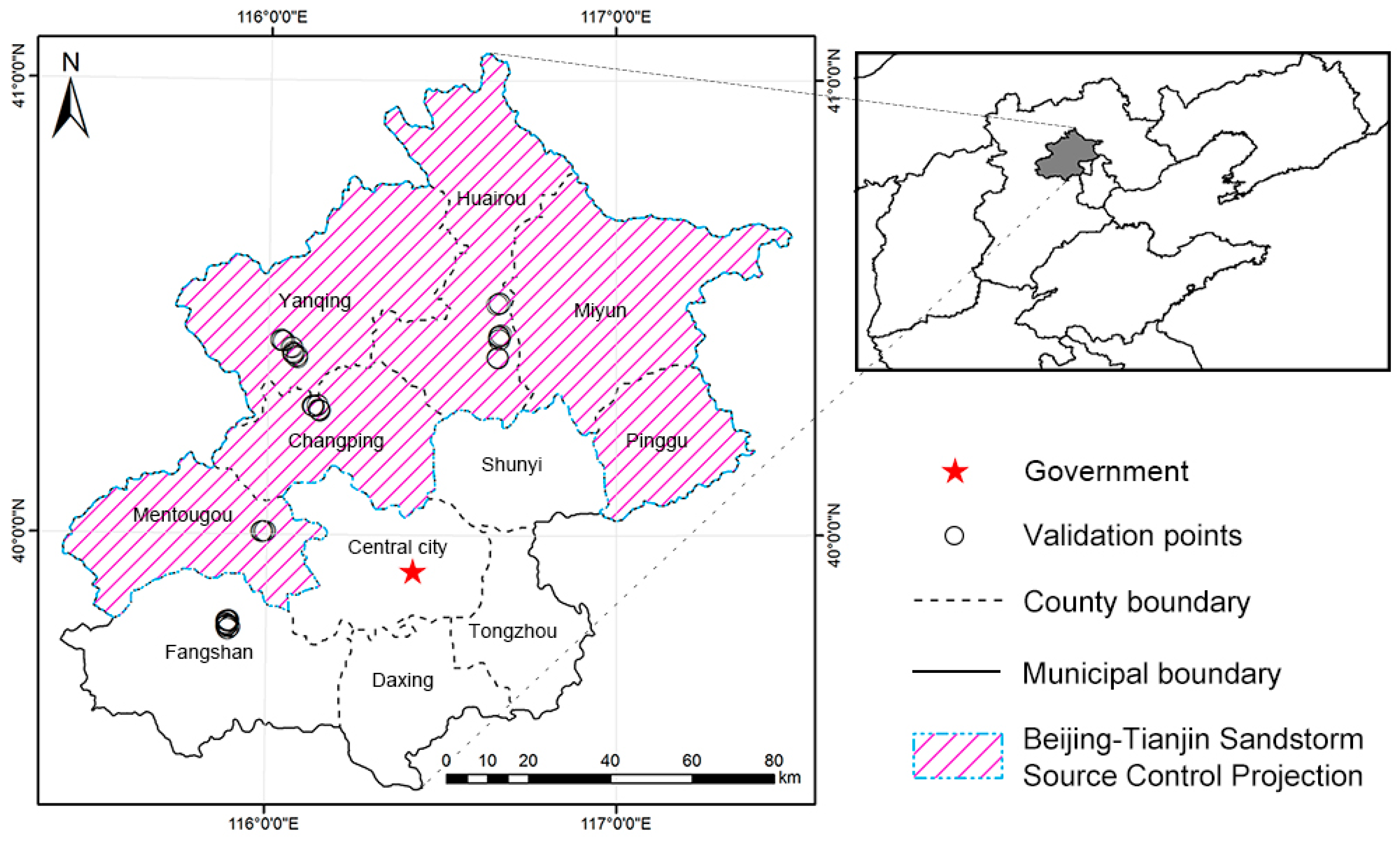
2.1. Study Area

Shielded by the Yan Mountains, Beijing is located in the north of the North China Plain (115.7°–117.4°E, 39.4°–41.6°N). The center is at 39°54′20″N, 116°25′29″E (Figure 1). Beijing spans over 160 km (EW) and 176 km (NS), including 16 districts and counties that are adjacent to the provinces Tianjin and Hebei. The flatland accounts for 1/3 (6390.3 km2) and the mountain land accounts for 2/3 (10,417.5 km2) of the total area (~16,353.2 km2). The climate in Beijing is the typical North Temperate Zone semi-humid continental monsoon climate with hot and rainy summers, cold and dry winters, and a short spring and autumn. The distribution of seasonal precipitation is uneven, with 80% of the annual precipitation occurring in June, July, and August. The annual average sunshine duration is approximately 2000–2800 h. Distributed in the north and west, the vegetation resources of Beijing are mainly warm temperate deciduous broad-leaved forests, and occasionally, temperate coniferous forests. Most of the plain has already been turned into farmlands and towns.

2.2. Data Sources and Pre-Processing

Landsat-5 TM and Landsat-8 OLI ortho-images with a spatial resolution of 30 m from four periods (2000, 2005, 2010, and 2015) were downloaded at no cost from USGS (http://earthexplorer.usgs.gov), the Institute of Remote Sensing and Digital Earth, Chinese Academy of Sciences (http://eds.ceode.ac.cn) and Geospatial Data Cloud, Computer Network Information Center, CAS (http://www.gscloud.cn). All images were obtained during July or August, covering less than 2% clouds. These images were processed as level 1T (precision and terrain corrected) products, so we completed pre-processing, including radiometric calibration, FLAASH atmospheric correction, and ortho-rectification. Previous studies have suggested that Landsat-8 OLI data show biased values, especially in bands RED and NIR, in comparison with TM data [29,30]; therefore, we completed histogram matching between OLI and TM to make the radiation values of the multi-source images comparable. We also used the same atmospheric correction method for all Landsat data, as well as using the same selectable calibration parameters, which might help alleviate the bias [30]. We created mosaics for the 3-scene or 4-scene images (path/row: 122/32, 123/32, 123/33, and 124/32) of each period using seamless mosaics in ENVI 5.1, which allowed finer image control and a better fusion of the image edges. The land cover data with 30m resolution was supplied by the National Geomatics Center of China (http://www.globallandcover.com). The 2000–2015 Beijing statistical yearbooks provided the socioeconomic data (e.g., GDP, population) [31]. Time series of annual climate data were also obtained from the statistical yearbooks, which were derived from the observation data from the Beijing Meteorological Bureau and calculated by the Beijing Statistical Bureau. Multi-year annual mean climate data were offered by the National Meteorological Information Center (http://data.cmc.cn).
To validate the accuracy of the FVC results from remote sensing, field FVC data was acquired based on the visual estimation method in June and August 2015, in Beijing. Considering the distance convenience, vegetation distribution, feasible fieldwork time in the growing season, and staff limitation, we carried out field work in vegetated areas such as Huairou, Yanqing, Changping, Mentougou, and Fangshan. In total, 63 sample plots were obtained, in which vegetation was distributed evenly. The size of each plot was 100 m × 100 m, with two 30 m × 30 m sample squares. Three individuals were used to estimate the FVC in each sample square. They walked along the two diagonal lines of each sample square and recorded 1 or 0, to represent the presence or absence of vegetation cover, and the vegetation coverage on the two diagonal lines was calculated separately. The process was repeated three times by the three individuals, and the arithmetic average value was taken as the total coverage of one sample square. The mean FVC of the two sample squares was regarded as the true FVC of each sample plot, which was intended to improve the reliability of the in-situ data and better match the scale of the Landsat data. A Trimble GPS was used to record the coordinates for the center of the sample plots, and each plot was visually estimated by three people. The plot design is shown in Figure 2. We used the conventional standard deviation analysis method to exclude the abnormal points ( | x μ | > 2 σ , x is the value of the point, μ is the mean value of all points, and σ is the standard deviation of all points), maintaining 60 sample plots as accuracy validation points. These points were distributed in the urban areas (seven points), suburban areas (17 points), and mountainous areas (36 points) of Beijing (Figure 1).

2.3. Methodology

2.3.1. Dimidiate Pixel Model

A pixel is generally considered to contain various surface features information. Therefore, by establishing a spectral mixture model, we can confirm that each surface features a ratio of one pixel. There is a generalizability approach of the linear spectral mixture method, the dimidiate pixel model (DPM). For our research, that only aims to analyze regional FVC values, this model has a simple algorithm and a strong operability. Additionally, it can weaken the influence of the atmosphere, soil background, vegetation types, etc. [32]. Many studies indicated that this model was suitable for diverse vegetation types and resolutions of remote sensing data [33,34,35,36,37].
In the dimidiate pixel model, we hypothesized that a pixel was only composed of vegetation and non-vegetation information. The observed information of one pixel was expressed as S, while the vegetation information was expressed as Sv, and the non-vegetation information was Sn:
S = S v + S n
The ratio of the vegetation coverage area to the total area in a pixel was the FVC of this pixel (fc). The ratio of the non-vegetation coverage area to the total area in a pixel was 1 − fc. We hypothesized that the pure pixel information that was completely covered by vegetation was Sveg, and the non-vegetation-covered pixel information was Snon. Then, Sv can be expressed as the product of fc and Sveg:
S v = f c × S v e g
In a similar way, Sn was the product of 1 − fc and Snon:
S n = ( 1 f c ) × S n o n
The fc value was deduced as follows:
S = S v + S n = f c × S v e g + ( 1 f c ) × S n o n
f c = S S n o n S v e g S n o n
Rundquist performed linear correlation analysis of FVC and NDVI, affirming that there was a good correlation between them [38]. Wittich and Hansing’s achievements demonstrated the indicative function of NDVI to FVC [39]. NDVI was the most widely applied indicator to vegetation growth [40,41,42,43,44]. Substituting NDVI into Equation (5), the FVC expression was derived as follows:
F V C = N D V I N D V I n o n N D V I v e g N D V I n o n
NDVInon was an NDVI value in the non-vegetation-covered area, i.e., the NDVI of a non-vegetation pixel should be 0 in theory; NDVIveg represented the NDVI value of the pixel that was fully covered by vegetation, i.e., the NDVI of a pure vegetation pixel should be 1. However, in practice, NDVInon was −0.1–0.2 because it was affected by noise [38,45]. Similarly, NDVIveg was usually not 1. Li believed that NDVIveg and NDVInon should be determined by the image itself, which can eliminate various interferences of the image [32]. In this paper, we chose the NDVI value in the NDVI frequency histogram of the image corresponding to a cumulative frequency with the value of 1% as the NDVInon, and 99% as NDVIveg.

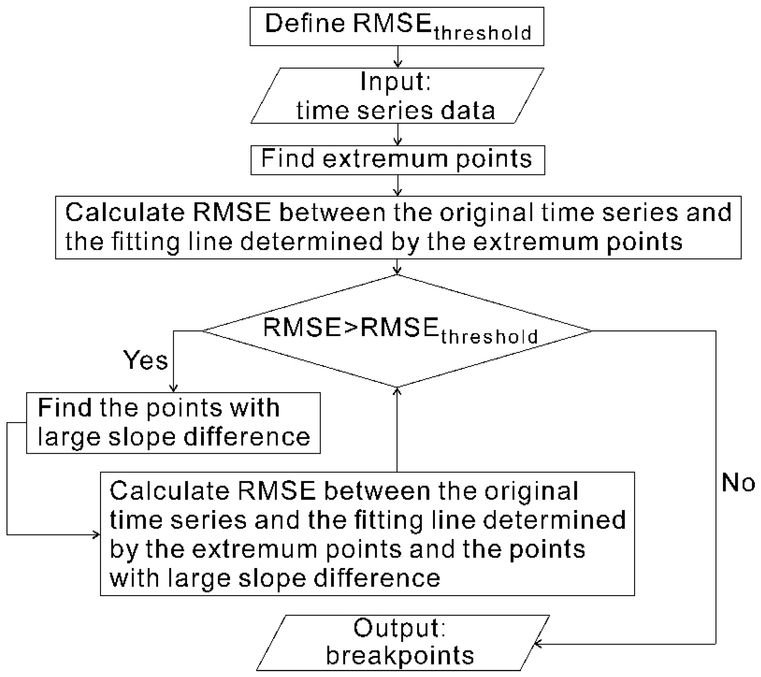
2.3.2. Piecewise Linear Regression

Piecewise linear regression (PLR) is a commonly applied method for reflecting variations in a time series [46]. PLR divides time series data into multiple adjacent fitting lines with the minimum root mean square error [47]. In this study, we were not only limited to choosing extremum points as key breakpoints, but we also calculated the differences of every two adjacent sequence segment slopes, to acquire a high degree of goodness of fit. The specific procedure for determining the breakpoints is shown below (Figure 3).

2.3.3. Bivariate and Partial Correlation Analysis

To quantitatively analyze the correlation between vegetation changes and socioeconomic factors, we used bivariate (Equation (7)) correlation analysis to calculate their correlates, as shown by Pearson correlation coefficients (r). The coefficient of determination R2 equaled r square. In the equations, x represents the socioeconomic factors and y represents the average FVC.
r x y = R 2 = i = 1 n ( x i x ¯ ) ( y i y ¯ ) i = 1 n ( x i x ¯ ) 2 i = 1 n ( y i y ¯ ) 2
However, there were intensive interactions between each factor [48]. When there are other variables affecting the correlation analysis results, bivariate correlation analysis may not be able to identify a positive or negative relationship. Thus, we used partial correlation analysis (Equation (8)), excluding the controlled variables, to measure the relationship between the two variables, without other influential factors.
r x 1 y ,   x 2 = r x 1 y r x 1 x 2 r x 2 y 1 r x 1 x 2 2 1 r x 1 y 2

2.3.4. Factor Analysis

Factor analysis (FA) is an important dimensionality reduction method promoted from principal component analysis to simplify multiple complex variables. Assuming that a multivariate system can be described by n random variables [x = (x1, x2, ..., xn)’], the mathematical model of FA is as follows:
x μ = AF + ε
Μ = (μ1, μ2, ..., μn)’ is the mean value, A = (αij) is the loading matrix, F is the common factor, ε is a special factor, and Var is variance. The factor contribution can be calculated as follows:
Contribution   =   i   =   1 n α i j 2 i   =   1 n V a r ( x i )

2.3.5. FVC Growth Rate

To clearly show the transitions of vegetation greenness in the time series, we calculated the growth rates of the mean FVC using Equation (11).
Rate = A 2 A 1 A 1 × 100 %
A2 represents the mean FVC of the last year, while A1 represents the mean FVC of the initial year.

3. Results

3.1. FVC Estimation Results

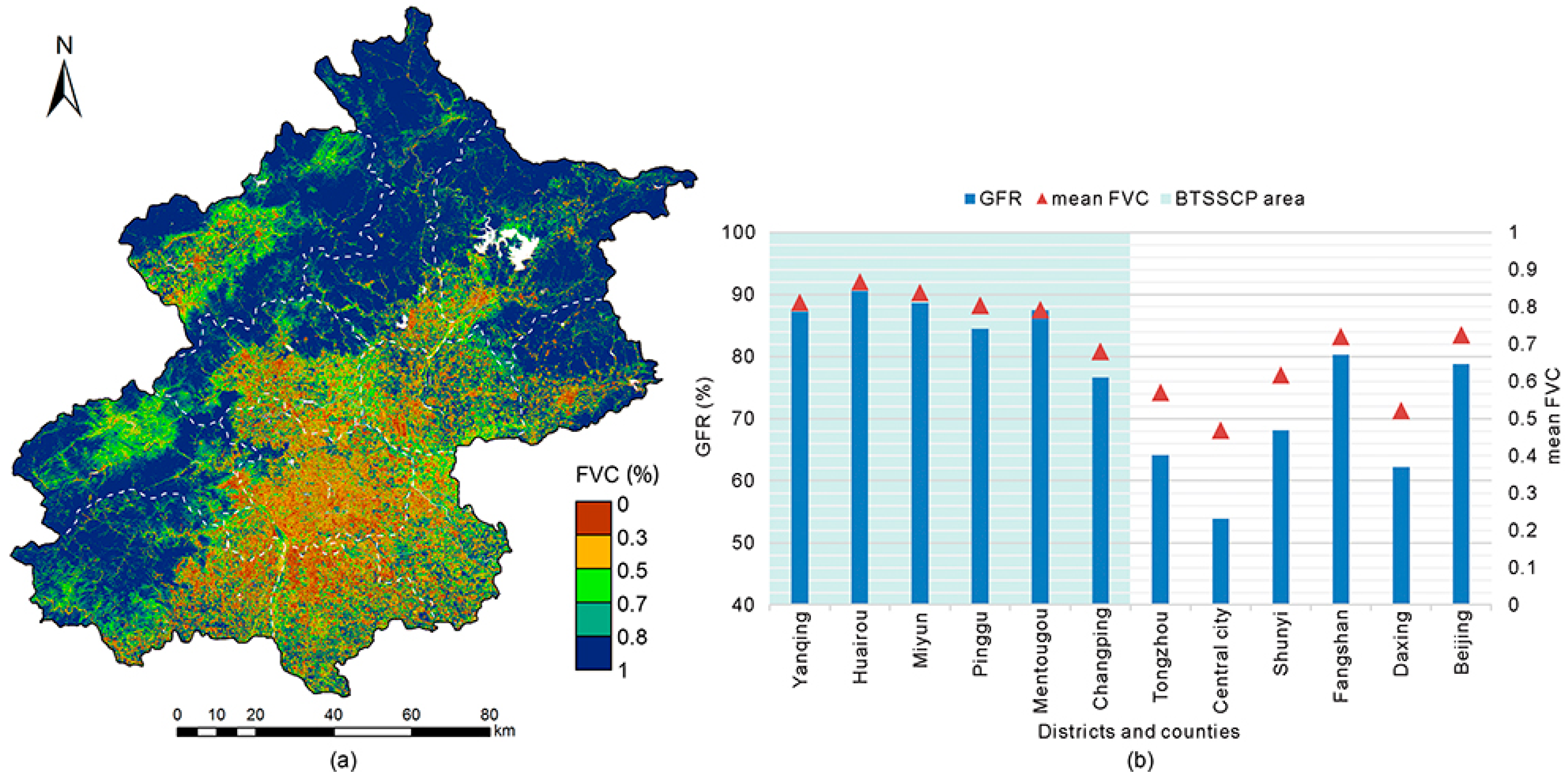
3.1.1. Spatial Distribution of FVC

Figure 4 shows the FVC in Beijing for 2015. As shown in the figure, the high FVC is mainly distributed in the north and west, and the low FVC is mainly seen in the urban areas. The mean FVC for the entire city of Beijing was 0.725; the higest FVC was 0.867 in Huairou, and the lowest was 0.468 in Central city. The sub-areas of Beijing were ranked by the mean FVC in descending order, as: Huairou > Miyun > Yanqing > Pinggu > Mentougou > Fangshan > Changping > Shunyi > Tongzhou > Daxing > Central city. We also classified the FVC estimation data into five levels using the Natural Breaks method, which best minimizes within class differences and maximizes between class differences [49]; rankings of 1 to 5 indicate poor, relatively poor, moderate, relatively good, and good, as shown in Table 1. Based on the in-situ investigation and the land use map, we placed rankings 3, 4, and 5 into the “good FVC” category, and rankings of 1 and 2 into the “bad FVC” category. We calculated the “good FVC” ratio (GFR) at district and county level to further show the vegetation conditions of Beijing. The GFR of Beijing was 78.8%; the highest and the lowest GFR were in Huairou and Central city (90.5% and 53.8%, respectively). The sub-areas of Beijing were ranked by GFR in descending order, as: Huairou > Miyun > Yanqing > Mentougou > Pinggu > Fangshan > Changping > Shunyi > Tongzhou > Daxing > Central city.

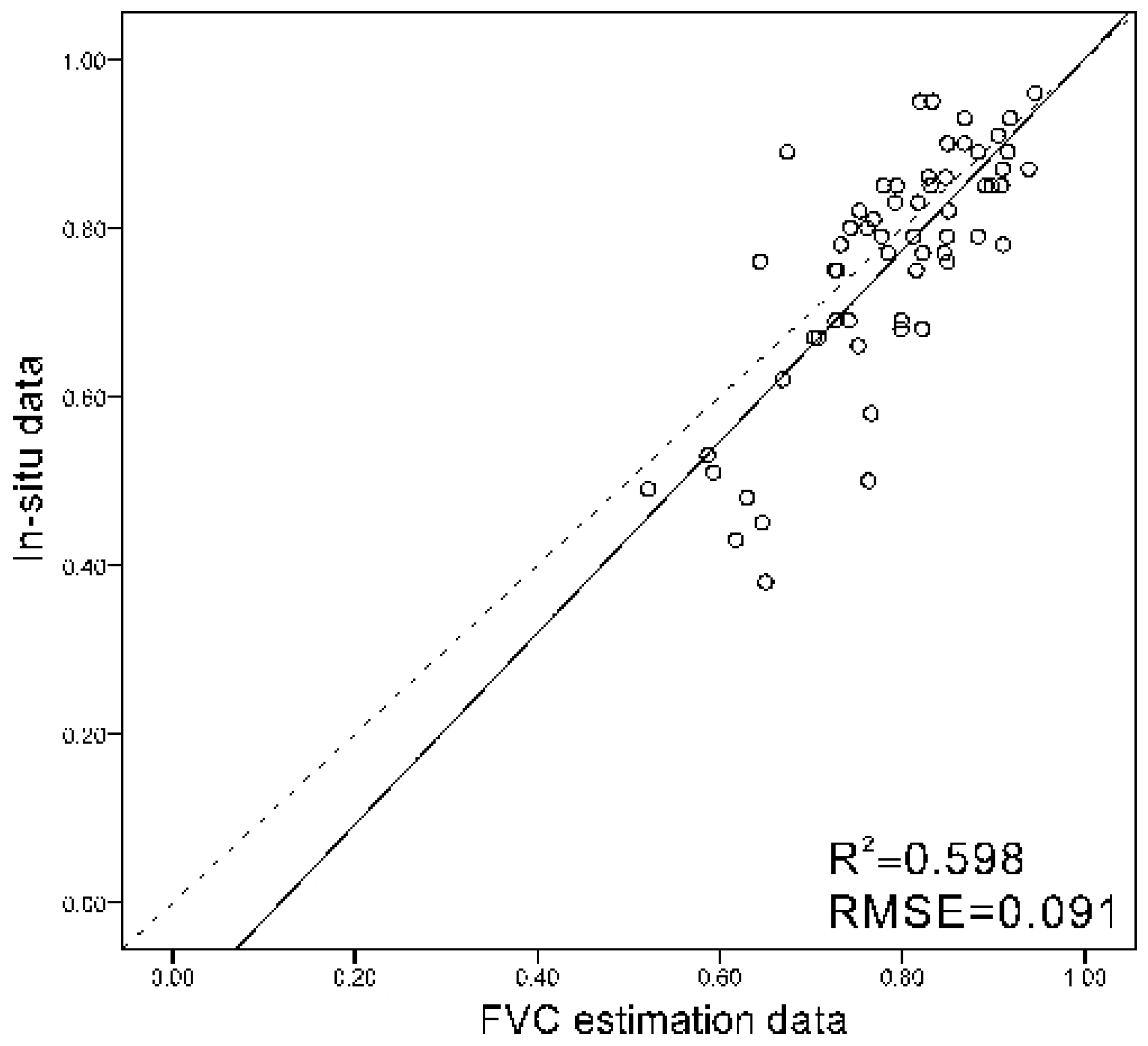
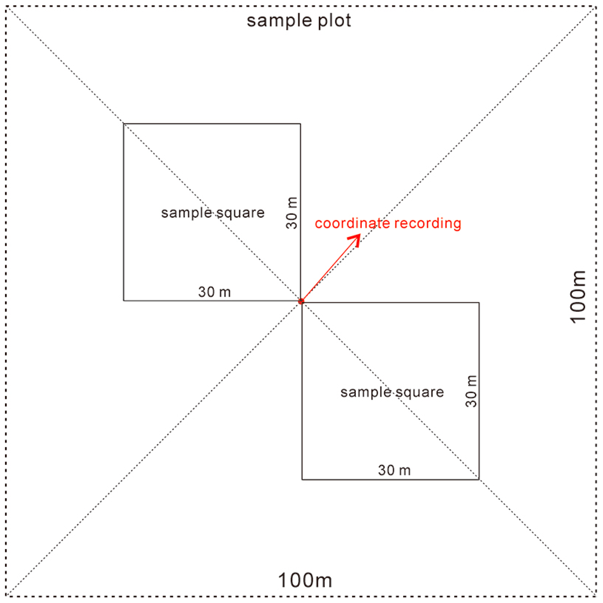
3.1.2. Accuracy Validation

To validate the accuracy of the results in our study area, the 60 in-situ checkpoints were utilized to perform a bivariate correlation analysis with the FVC estimation data. The Pearson’s correlation coefficient was 0.773 (p < 0.01, RMSE = 0.091), which meets the accuracy requirements (Figure 5), indicating that the DPM was reliable in extracting the FVC. This is also consistent with previous findings [3].

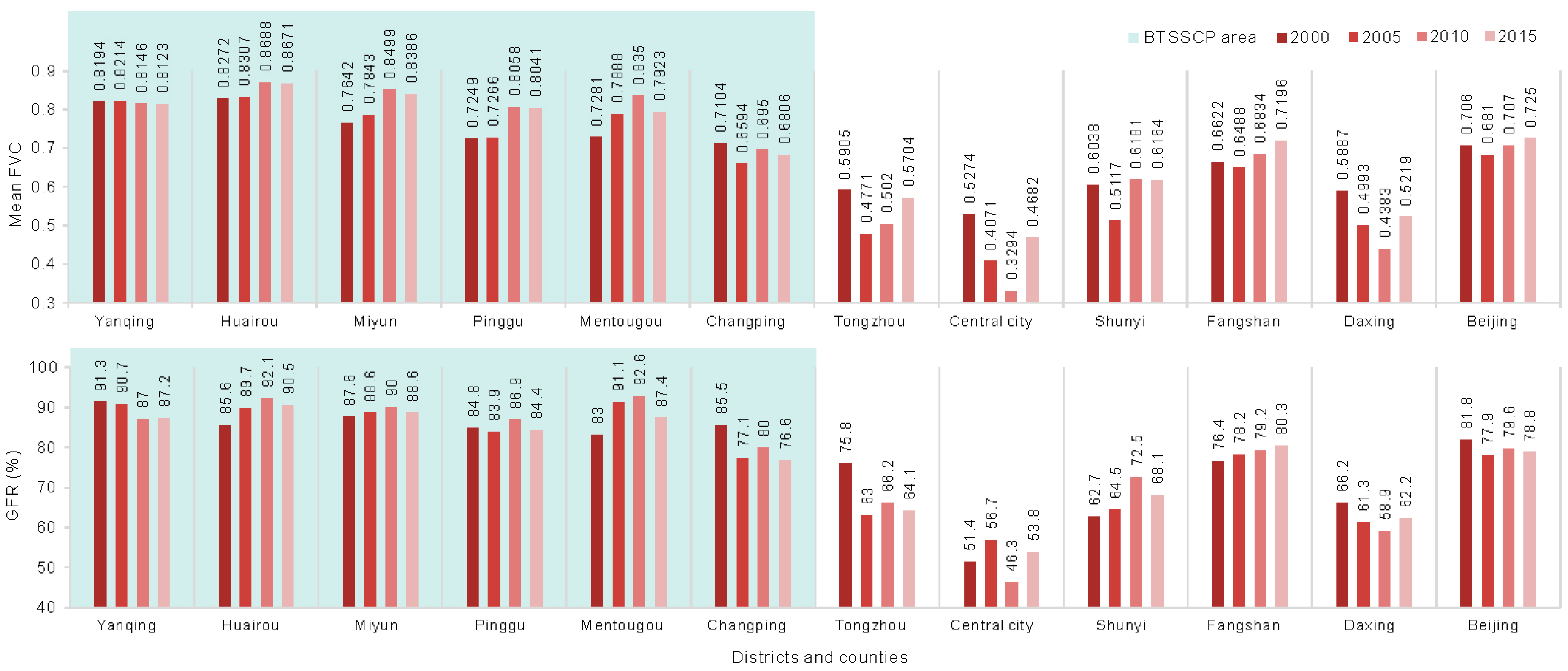
3.2. Spatial-Temporal Variation of FVC during 2000–2015

Figure 6 illustrates the temporal characteristics of the FVC, indicating that the general restoration of vegetation greenness from 2000 to 2015 occurred in Huairou (HR), Miyun (MY), Shunyi (SY), Pinggu (PG), Mentougou (MTG), and Fangshan (FS); the degradation of vegetation coverage was seen in Yanqing (YQ), Changping (CP), Tongzhou (TZ), Daxing (DX), Central city (CC), and the whole of Beijing.
We used the minus tool of spatial analyst tools in ArcGIS 10.2 to carry out difference calculations by subtracting the FVC estimation data of the former period from the latter, and made three spatial vegetation restoration and degradation pattern maps (Figure 7) for 2000 to 2005, 2005 to 2010, and 2010 to 2015. The difference values were between −1 and 1. Based on our field investigation and magnitude of the difference values, we defined −1 to −0.2 as significant degradation, shown in maroon; −0.2 to 0.2 was defined as non-significant change, shown in off-white; and 0.2 to 1 was defined as significant restoration, shown in green.
Combining Figure 6 and Figure 7, from 2000 to 2005, the ratio of the significant restoration area was 6.33%, while the ratio of the significant degradation area was 13.62%. The main greening area was in MTG; CP, SY, TZ, and CC were in browning. In the next five years, from 2005 to 2010, the ratio of the significant restoration area increased by 3.75% (to 10.08%), and the ratio of the significant degradation area decreased by 4.27% (to 9.35%). SY, CP, and TZ were then in greening, while CC was still in browning. From 2010 to 2015, the ratio of the significant restoration area increased by another 2.73% (to 12.81%), and the ratio of the significant degradation area remained generally stable (9.49%). During this period, YQ, and the most non-BTSSCP area, was in greening. The main degradation area was in the northern MTG area. It is verified that Beijing experienced both restoration and degradation from 2000 to 2015, and the vegetation conditions were better in general, only partially deteriorating.

3.3. Correlations between Climatic Factors and FVC

Time series of the annual mean temperature (AMT) and annual total precipitation (ATP) data were taken from Beijing statistical yearbooks. From 2000 to 2015, the AMT decreased by −0.0032 °C·year−1 (R2 = 0.12, p = 0.185), while the ATP significantly increased by 0.0323 mm·year−1 (R2 = 0.45, p = 0.005) (Figure 8). The PLR method divided the time series of AMT into three different trends (two breakpoints): 2000 to 2006, 2007 to 2010, and 2011 to 2015. From 2000 to 2006, the AMT significantly increased at a rate of 0.0077 °C·year−1 (R2 = 0.60, p = 0.041), whereas from 2007 to 2010, it significantly decreased at a rate of −0.0345 °C·year−1 (R2 = 0.94, p = 0.032); a significantly decrease also took place during 2011 to 2015, at a rate of −0.0232 °C·year−1 (R2 = 0.95, p = 0.005) (Figure 8a). The PLR method also divided the ATP time sequence into three trends: 2000 to 2005, 2006 to 2011, and 2012 to 2015. Before 2006, the ATP slightly increased, at a rate of 0.0204 mm·year−1 (R2 = 0.59, p = 0.12); from 2006 to 2011, it increased at a rate of 0.1778 mm·year−1 (R2 = 0.59, p = 0.074); and it decreased after 2012, by −0.0656 mm·year−1 (R2 = 0.32, p = 0.431) (Figure 8b). The data show that in 2005/2006, there was a drought in Beijing, which was agreeable with the research conducted in Northern China [50,51]. However, in 2011/2012, although the temperature increased, the precipitation was abundant.
Multi-year annual mean climate data from eighteen meteorological stations were selected to be the parameters for the bivariate and partial correlation analysis with FVC at a spatial level. The multi-year monthly temperature and multi-year monthly precipitation data from April to October were chosen to calculate the multi-year annual mean temperature (MAMT) and multi-year annual mean precipitation (MAMP) in the growing season [52]. Table 2 shows the results. In the bivariate correlation analysis, the MAMT showed a significant negative relationship with FVC (r = −0.69, p = 0.019), but the MAMP did not (p > 0.05). To better confirm the relationships between each climate factor and FVC, a partial correlation analysis was performed. The results showed that the FVC was significantly negatively correlated with the MAMT (r = −0.819, p = 0.004); the FVC was significantly positively correlated with the MAMP (r = 0.653, p = 0.04).

3.4. Correlations between Human Activities and FVC

3.4.1. Beijing-Tianjin Sandstorm Source Control Project

BTSSCP is a sandstorm control policy which was implemented in Beijing, Tianjin, Hebei, Shanxi, and Inner Mongolia from 2000 to 2010. From 2000 to 2005, 2005 to 2010, 2000 to 2010, and 2010 to 2015, the percentages of the significant restoration area of BTSSCP accounted for 5.43%, 3.07%, 11.45%, and 1.88%, respectively; the percentages of the significant degradation area were 1.6%, 1.11%, 7.53%, and 5.68%, respectively The percentages of the significant restoration area of non-BTSSCP accounted for 9.82%, 13.34%, 13.09%, and 11.34%, respectively; the percentages of the significant degradation area were 8.95%, 4.74%, 32.83%, and 6.09%, respectively (Table 3). In the three five-year periods (2000–2005, 2005–2010, and 2010–2015), the restoration or degradation area of BTSSCP was relatively small, while the restoration or degradation area of non-BTSSCP was relatively large. This was mainly because, in the year 2000, the mean FVC of BTSSCP (0.77) was much higher than non-BTSSCP (0.6); the cardinal number was large, so the significant restoration area (FVC increased more than 0.2) ratio was small in the BTSSCP area.
The total effectiveness is a parameter for comparing the ecological conservation and restoration efforts in various ecological conservation areas (BTSSCP and non-BTSSCP in our study), which can be analogized as: Total   Effectiveness = Restoration + Stable Degradation . The total effectiveness is higher if the Restoration and Stable values are larger, and the Degradation value is smaller. The total comparative effectiveness of ecological restoration efforts can be ranked using the total effectiveness [25]. In every five-year period, the total effectiveness of the BTSSCP area (96.79, 97.77, and 88.63, respectively) was better than the non-BTSSCP area (82.09, 90.52, and 87.83, respectively). Moreover, from 2000 to 2010, the total effectiveness of the BTSSCP area (84.94) was much higher than that of the non-BTSSCP area (34.34). Based on these facts, we can conclude that during the BTSSCP implementation period (2000–2010), the vegetation conditions of the BTSSCP area were well maintained. These findings are consistent with previous studies, which showed that the ecological policy was very effective in improving the vegetation conditions [44,53].

3.4.2. Socioeconomic Factors

We chose some related available socioeconomic variables at a district and county level for a bivariate-partial correlation analysis with vegetation transitions and factor analysis. These included the total population, GDP, Engel coefficient of urban, Engel coefficient of rural, per capita consumption of urban and per capita consumption, and investment in fixed assets (a significant indicator of urban expansion [54]).
Table 4 presents the correlation coefficients and significance between the overall vegetation coverage changes and socioeconomic factors. In the bivariate correlation analysis, FVC showed a significantly negative correlation with the total population (r = −0.705, p < 0.001), GDP (r = −0.556, p < 0.001), the Engel coefficient of urban (r = −0.537, p < 0.01), and the investment in fixed assets (r = 0.443, p = 0.01). In the partial correlation analysis, the controlled variables were removed, and FVC only maintained a significantly negative correlation with the total population (r = −0.684, p < 0.05); however, the partial correlation coefficient with GDP was only −0.125 and did not pass the t-test.
The most contributory socioeconomic factors tested by factor analysis were the population (contribution = 54.356%) and GDP (contribution = 30.677%). The question arose as to why GDP showed such a difference in the bivariate and partial correlation analyses. To confirm whether there was some relationship between GDP and vegetation changes, we drew a scatter plot of GDP-FVC (Figure 9a) at a district and county level, and also drew a population-FVC scatter plot, used for comparison (Figure 9b). It was observed that the points of TZ, DX, CC, FS, SY, and CP (T-C) are distributed on the left of the vertical dashed line, which represents “mean FVC = 0.7”. The points of HR, MY, PG, MTG, and YQ (H-Y) were distributed on the right of the dashed line. There are possible different relationships on the left and right. Figure 9c,d show the FVC growth rates and population at a district and county level. Vertical dashed lines were illustrated to divide T-C and H-Y, and it could be seen that trends in FVC growth and population were spatially heterogeneous. In T-C, FVC growth was mostly negative, and the population increase was high and unstable. In H-Y, FVC growth was mostly positive, and the population increase was slight and stable. These phenomena would be manifested, based on different policy contexts. Therefore, we proposed a hypothesis that the correlation between socioeconomic factors and vegetation changes might be spatially heterogeneous, based on the context of different areas.
According to our hypothesis, the correlation coefficients of GDP-FVC and population-FVC in T-C and H-Y were calculated, respectively (Table 5). Although there were two obvious groups of points divided by the vertical line FVC = 0.7, and the plus-minus signs of coefficients in T-C (r = −0.175 in bivariate, r = 0 in partial) and H-Y (r = 0.066 in bivariate, r = −0.325 in partial) were opposite, the significance of population-FVC shows that there was no statistical significance of population-FVC in T-C or H-Y (p > 0.1), so the influence of population was not spatially heterogeneous, based on our data. However, there were two opposite trends in the correlation analysis of GDP-FVC in the two groups of points. In T-C, the GDP showed a significantly negative correlation with FVC (r = −0.601, p < 0.01), and a significantly positive correlation with H-Y (r = 0.614, p < 0.01).

4. Discussion

4.1. Possible Influential Factors for Vegetation Change Trends

Lü et al., Tian et al. and Feng et al. pointed out that both natural and human-induced factors have effects on vegetation change, but human-induced factors are more significant in explaining trends [25,55,56]. In this paper, the correlation between the temperature and precipitation, and the FVC, are both significant, and the correlation coefficient between temperature and FVC is higher. From these results, it seems that temperature is inhibiting the growth of vegetation. However, it is well known that this phenomenon occurs in arid and semi-arid areas, with less precipitation [22]. The total precipitation in Beijing is 500–600 mm per year, which makes Beijing a semi-humid region. Furthermore, a 16-year period is a short-term series, and there were also no extreme climatic events, so the meteorological conditions should be seen as a stable condition. Therefore, the climatic factors can not be used to explain the changes in vegetation.
In stable meteorological conditions, human activity is a very significant factor in impacting vegetation changes, especially in mega cities, and the intense human activity can change the urban environment over a short period [57], which has been a hot issue of international concern in recent years. Considering that Beijing is a rapidly developing region with very severe human activity influences, we try to explore whether the strong correlation between climate and FVC is influenced by human activities. Peng et al. found that in Eastern China, the mean NDVI values in the urban areas were lower than those in the rural areas, which suggested that anthropogenic activities in the urban area would have more influence on the vegetation density, manifesting as a decrease in the mean NDVI [27]. This was consistent with the results of our study. The results of the ecological project effect show that, before 2010, namely the implementation period of BTSSCP, in spatial, the total effectiveness of the BTSSCP area was higher than that of non-BTSSCP area, directly showing that human afforestation activities can effectively improve the ecological environment. After 2010, the main degradation area was in MTG. In the second investigation of Chinese land resources in 2007, the type of vegetation in the main degradation area was grassland, but it was transformed to sparse shrub in 2015, according to our investigation. We therefore believe that it is the main contribution to the reduction of total effectiveness in the BTSSCP area. During this period, there was also a large scale plain afforestation project (between the year 2012 to 2015) being rapidly implemented in the non-BTSSCP area. Hence, the total effectiveness of the non-BTSSCP area is also considerable. These facts may not be highly consistent with the expectations, but it is further explained that human-induced policies had significant impacts on vegetation changes. Besides, Sun et al. also proposed that the ecological conservation and restoration policies such as BTSSCP have improved vegetation in the mountainous area of Beijing, and the urban green space construction policies such as plain afforestation project and the preparation for the Olympics have increased the vegetation coverage in the plain urban area [58]. In the correlation analysis of socioeconomic factors with FVC, the relationships are very significant, which are also significant in explaining ecological transitions [57]. How human activity impacts are exerted is another important focus of this study.

4.2. Spatial Heterogeneity of Human Activity Influences

On the basis of our hypothesis, another new point that our study concentrated on was the spatial heterogeneity of human activity influences. Wang et al. criticized the negative effects of economic development on the environment in Southeast China, but it was based on a fast-growing population, which was inconsistent with our study [59]. Table 6 shows that, in most parts of the BTSSCP area, there were positive trends in the vegetation growth; for the aspects of society and economy, there was a stable increase in population, and the GDP showed a positive relationship with vegetation change. This indicated that, although the population was increasing, it increased at a slow rate and was under control, so the increasing population did not obviously damage the local ecosystem in the BTSSCP area. The positive effects of economic welfare and ecological restoration projects were much more significant, which improved the local ecosystem. An empirical study in China from 2000 to 2010 also proved that regional economic welfare may have generally significant positive impacts on vegetation greening [25]. Regression analyses in Italy and Nigeria also suggested that the economic productivity might contribute to ecological restoration and the mitigation of vegetation degradation [60,61].
On the contrary, in most parts of the non-BTSSCP area, negative trends in the vegetation growth were shown; a considerable increasing and fluctuation in the population also occured, while GDP became an indicator of urban expansion [62] and showed a negative correlation with vegetation change. In addition, there was no protection of ecological restoration projects. We therefore believed that in the non-BTSSCP area, the extensive growth and fluctuation of the population and urban expansion, the level of which reached the carrying capacity of ecosystems, caused negative effects on vegetation restoration. This is very common in developing countries [25] and could also be verified by empirical studies and case analyses. For example, Bangladesh experienced a decline in vegetation caused by population growth, economic development, and rapid urban expansion, from 1992 to 2003 [62], while in South Africa, the human population was strongly responsible for land cover change and degradation [63]. It proved that human activity influences would be highly spatially heterogeneous, based on the context of different areas. In addition, the analysis in the BTSSCP and non-BTSSCP areas indicated that vegetation restoration in the BTSSCP area over the last 16 years might be largely attributed to ecological projects, which is consistent with previous studies [44,53,64]. Taking the 2010 land cover data as a reference, what was in the non-BTSSCP area was mostly cultivated land and artificial surfaces, revealing that in this area, urban expansion and populations of great density and mobility brought destruction to the local ecosystem. Therefore, in order to restrain sand invasion and protect the ecosystem while expanding cities, an integrative consideration of ecological conservation, restoration policy, and the spatially heterogeneous of socioeconomic influences (on vegetation and the ecological system) is necessary, when governments make a decision.

4.3. Limitations and Future Work

It is important to consider that the impact of the soil background would introduce errors to the estimation of FVC. There was a shortcoming when using the NDVI, with a response effect inconspicuous to highly-vegetation-covered areas. When the FVC is smaller than 15%, the NDVI can differentiate the soil and vegetation, but when the FVC is larger than 80%, the capacity of the NDVI response to vegetation is weak [65,66,67]. The visual angle in FVC definition was vertical to the surface, but when the satellite sensor acquired remote sensing data, the angle was normally not vertical to the ground. In general, the sensor angle was related to the sensor type. This could also cause errors when estimating the FVC [32]. We could not obtain remote sensing images each year with identical phases, and we also could not remove all the clouds without replacing them with other parts of images. Therefore, the existence of different phases in our images inevitably introduced errors.
Our study area was the city of Beijing. Considering its area and the time period of the study, we chose 30-m Landsat data to conduct the research. The advantages of Landsat data were that the historical data was available, the data volume was moderate, and the resolution also met the in-situ sample resolution and research requirements. However, the data provided by USGS was not continuous in the time sequence, which was very limiting for our research. From many images, we chose the years 2000, 2005, 2010, and 2015 as the four time nodes of Beijing vegetation coverage for estimating and monitoring, and because the time resolution was low, we could not conduct trend analysis using the least square method, which has a higher statistical accuracy. We could only perform difference calculations, which can show vegetation growth trends, but cannot identify the significance level, so there was a weakness in the statistics. Furthermore, because the sample sizes of socioeconomic and meteorological data that we could obtain were significantly different from the size of the remote sensing images, combined with the lack of certain socioeconomic or meteorological data at a district and county level or at a time sequence, uncertainties were brought into the statistical test that affected the accuracy [68]. This meant that the analysis results of some indices could not pass the t-test. In future work, our study will be not limited to four separate years, a 16-year study period, or one city. We would like to use year-by-year remote sensing data, more comprehensive socioeconomic and meteorological data, and consider a longer time period and wilder study area to verify our current findings. In addition, indicators of vegetation conditions would not only be limited to FVC, and we would like to introduce other indices in the future, to indicate vegetation greenness.

5. Conclusions

This study monitored vegetation coverage changes from 2000 to 2015 in Beijing using remote sensing data and analyzed the correlative factors of the changes. The main conclusions of the study are as follows:
(1)
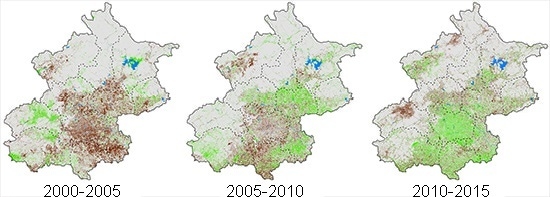
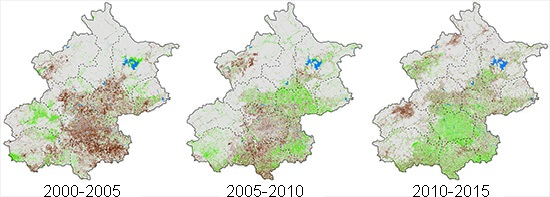
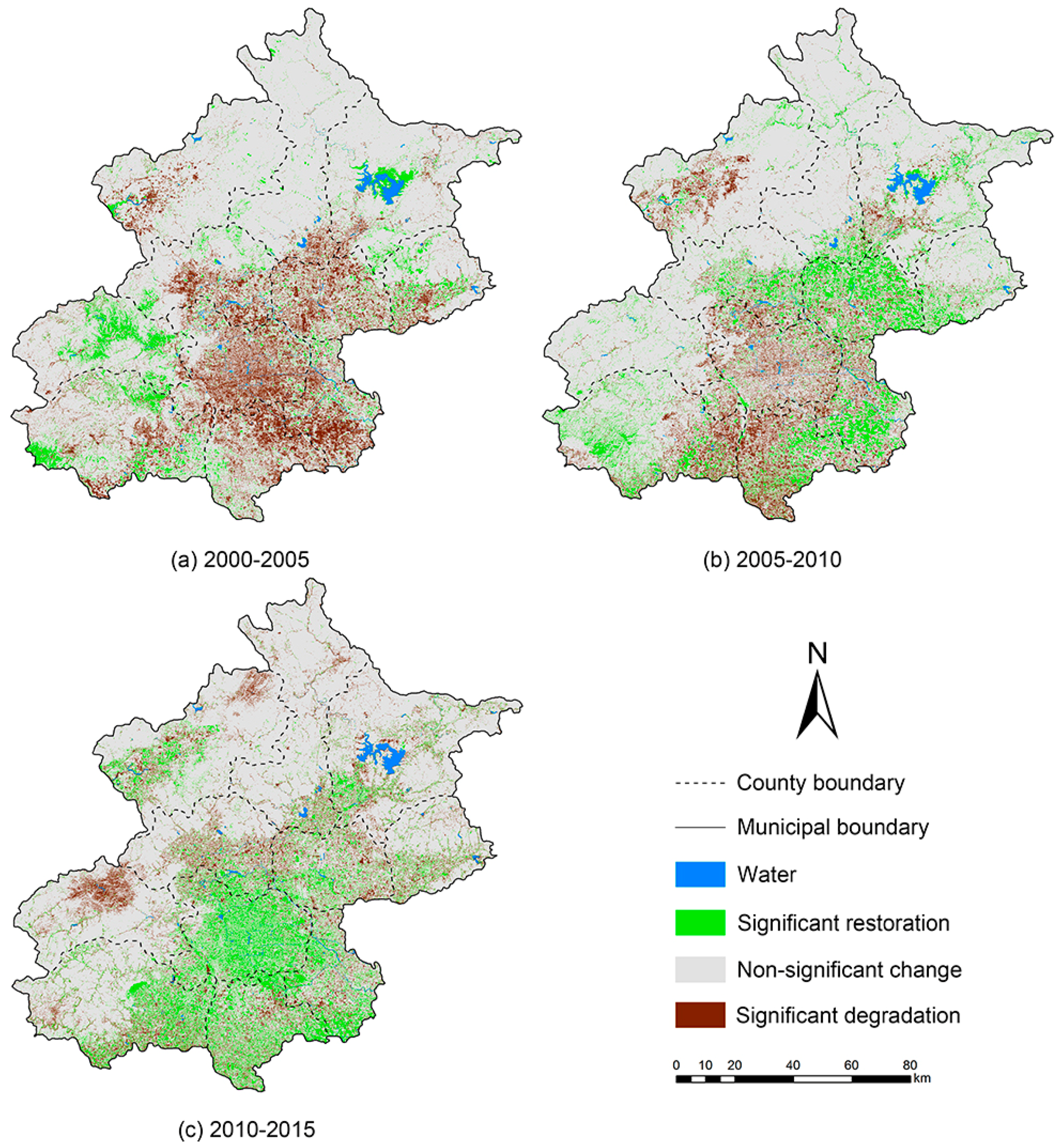
On an overall basis, from 2000 to 2005, 2005 to 2010, and 2010 to 2015, Beijing experienced both restoration (6.33%, 10.08%, and 12.81%, respectively) and degradation (13.62%, 9.35%, and 9.49%, respectively), the vegetation conditions were better in general, only partially deteriorating.
(2)
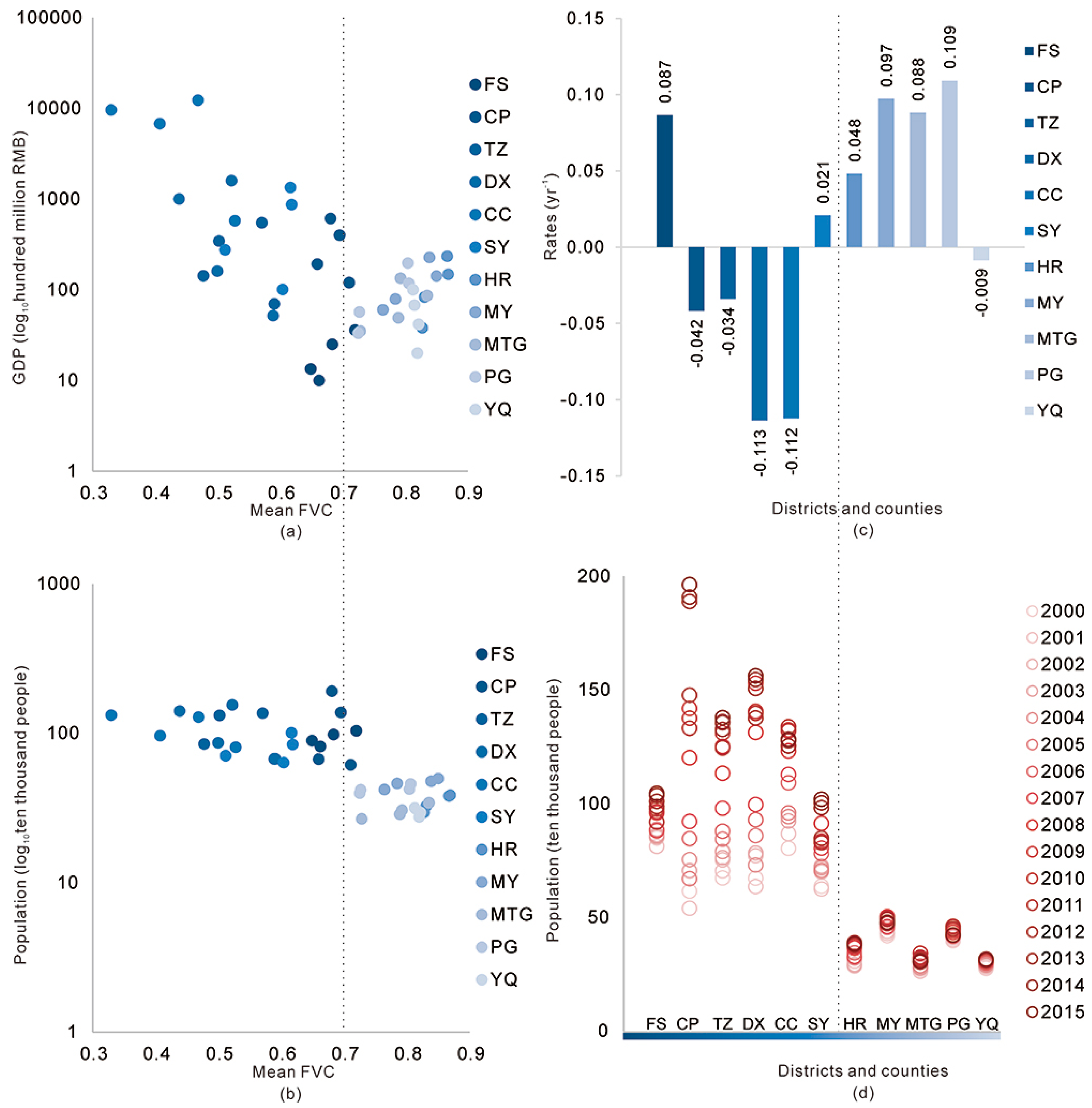
Human activity factors have significant relationships with vegetation cover changes, and they are a very significant factor in impacting and explaining vegetation changes. The socioeconomic factors, especially the population, were the dominant factors influencing the vegetation condition.
(3)
Human activity influences on vegetation coverage were highly spatially heterogeneous, based on the unique context of different areas, which needed to be evaluated comprehensively: in the BTSSCP area, the economic development and ecological restoration project improved the local ecosystem, based on a stable increase in population; in the non-BTSSCP area, the extensive growth and fluctuation of the population, urban expansion, and economic development, caused negative effects on vegetation restoration.

Acknowledgments

This study is supported by the China Geological Survey AGRS Center Project entitled "Comprehensive survey of natural resources in northern coastal areas by remote sensing (Beijing-Tianjin area)" ([2016]DD2016007709). We gratefully thank the constructive discussion with Yuan Zeng. We also thank Yongchao Zhao, Qiaomin Li, Yanqi Fang, and Chao He for the fieldwork. Chiayu Tung from New York University is specially acknowledged for language advice. We also want to thank the three anonymous reviewers and the guest editors for their suggestions that helped us to improve the manuscript.

Author Contributions

Shufang Tian, Qian Zhan, and Meichen Jiang conceived and designed the experiments; Meichen Jiang did the satellite imagery pre-processing and data analysis; Yuexin He, Zhaoju Zheng, and Meichen Jiang analysed the results; Zhaoju Zheng revised the paper; Meichen Jiang wrote the paper.

Conflicts of Interest

The authors declare no conflict of interest.

References

  1. United Nations. The Millennium Ecosystem Assessment; United Nations: New York, NY, USA, 2005. [Google Scholar]
  2. Ouyang, Z.; Zheng, H.; Xiao, Y.; Polasky, S.; Liu, J.; Xu, W.; Wang, Q.; Zhang, L.; Xiao, Y.; Rao, E.; et al. Improvements in ecosystem services from investments in natural capital. Science 2016, 352, 1455–1459. [Google Scholar] [CrossRef] [PubMed]
  3. Tong, S.; Zhang, J.; Ha, S.; Lai, Q.; Ma, Q. Dynamics of fractional vegetation coverage and its relationship with climate and human activities in Inner Mongolia, China. Remote Sens. 2016, 8, 776. [Google Scholar] [CrossRef]
  4. Dubovyk, O.; Landmann, T.; Erasmus, B.F.N.; Tewes, A.; Schellberg, J. Monitoring vegetation dynamics with medium resolution MODIS-EVI time series at sub-regional scale in Southern Africa. Int. J. Appl. Earth Obs. Geoinf. 2015, 38, 175–183. [Google Scholar] [CrossRef]
  5. Jiapaer, G.; Liang, S.; Yi, Q.; Liu, J. Vegetation dynamics and responses to recent climate change in Xinjiang using leaf area index as an indicator. Ecol. Indic. 2015, 58, 64–76. [Google Scholar]
  6. Kutiel, P.; Cohen, O.; Shoshany, M.; Shub, M. Vegetation establishment on the Southern Israeli Coastal sand dunes between the years 1965 and 1999. Landsc. Urban Plan. 2004, 67, 141–156. [Google Scholar] [CrossRef]
  7. Liu, T.; Yang, X. Mapping vegetation in an urban area with stratified classification and multiple endmember spectral mixture analysis. Remote Sens. Environ. 2013, 133, 251–264. [Google Scholar] [CrossRef]
  8. Tooke, T.R.; Coops, N.C.; Goodwin, N.R.; Voogt, J.A. Extracting urban vegetation characteristics using spectral mixture analysis and decision tree classifications. Remote Sens. Environ. 2009, 113, 398–407. [Google Scholar] [CrossRef]
  9. Matteucci, S.D.; Totino, M.; Arístide, P. Ecological and social consequences of the forest transition theory as applied to the Argentinean Great Chaco. Land Use Policy 2016, 51, 8–17. [Google Scholar] [CrossRef]
  10. Liu, Y.; Feng, Y.; Zhao, Z.; Zhang, Q.; Su, S. Socioeconomic drivers of forest loss and fragmentation: A comparison between different land use planning schemes and policy implications. Land Use Policy 2016, 54, 58–68. [Google Scholar] [CrossRef]
  11. Hansen, M.C.; Potapov, P.V.; Moore, R.; Hancher, M.; Turubanova, S.A.; Tyukavina, A.; Thau, D.; Stehman, S.V.; Goetz, S.J.; Loveland, T.R.; et al. High-resolution global maps of 21st-century forest cover change. Science 2013, 342, 850–853. [Google Scholar] [CrossRef] [PubMed]
  12. Hansen, M.C.; Stehman, S.V.; Potapov, P.V. Quantification of global gross forest cover loss. Proc. Natl. Acad. Sci. USA 2010, 107, 8650–8655. [Google Scholar] [CrossRef] [PubMed]
  13. Dymond, J.R.; Stephens, P.R.; Newsome, P.F.; Wilde, R.H. Percentage vegetation cover of a degrading rangeland from SPOT. Int. J. Remote Sens. 1992, 13, 1999–2007. [Google Scholar] [CrossRef]
  14. Gitelson, A.A.; Kaufman, Y.J.; Stark, R.; Rundquist, D. Novel algorithms for remote estimation of vegetation fraction. Remote Sens. Environ. 2002, 80, 76–87. [Google Scholar] [CrossRef]
  15. Zhang, W.; Fu, S.; Liu, B. Error assessment of visual estimation plant coverage. J. Beijing Norm. Univ. (Nat. Sci.) 2001, 37, 402–408. (In Chinese) [Google Scholar]
  16. Johnson, B.; Tateishi, R.; Kobayashi, T. Remote sensing of fractional green vegetation cover using spatially-interpolated endmembers. Remote Sens. 2012, 4, 2619–2634. [Google Scholar] [CrossRef]
  17. Zhang, X.; Liao, C.; Li, J.; Sun, Q. Fractional vegetation cover estimation in arid and semi-arid environments using HJ-1 satellite hyperspectral data. Int. J. Appl. Earth Obs. Geoinform. 2013, 21, 506–512. [Google Scholar] [CrossRef]
  18. Cao, Q.; Yu, D.Y.; Georgescu, M.; Han, Z.; Wu, J.G. Impacts of land use and land cover change on regional climate: A case study in the agro-pastoral transitional zone of China. Environ. Res. Lett. 2015, 10, 124025. [Google Scholar] [CrossRef]
  19. Wu, D.; Wu, H.; Zhao, X.; Zhou, T.; Tang, B.; Zhao, W.; Jia, K. Evaluation of spatiotemporal variations of global fractional vegetation cover based on GIMMS NDVI data from 1982 to 2011. Remote Sens. 2014, 6, 4217–4239. [Google Scholar] [CrossRef]
  20. Zhang, F.; Tiyip, T.; Ding, J.; Sawut, M.; Johnson, V.C.; Tashpolat, N.; Gui, D. Vegetation fractional coverage change in a typical oasis region in Tarim River watershed based on remote sensing. J. Arid Land 2012, 5, 89–101. [Google Scholar] [CrossRef]
  21. Tang, J.; Chen, F.; Schwartz, S.S. Assessing spatiotemporal variations of greenness in the Baltimore–Washington Corridor area. Landsc. Urban Plan. 2012, 105, 296–306. [Google Scholar] [CrossRef]
  22. Huang, K.; Zhang, Y.; Zhu, J.; Liu, Y.; Zu, J.; Zhang, J. The influences of climate change and human activities on vegetation dynamics in the Qinghai-Tibet Plateau. Remote Sens. 2016, 8, 876. [Google Scholar] [CrossRef]
  23. Sun, J.; Cheng, G.; Li, W.; Sha, Y.; Yang, Y. On the variation of ndvi with the principal climatic elements in the Tibetan Plateau. Remote Sens. 2013, 5, 1894–1911. [Google Scholar] [CrossRef]
  24. Feng, Q.; Ma, H.; Jiang, X.; Wang, X.; Cao, S. What has caused desertification in China? Sci. Rep. 2015, 5, 15998. [Google Scholar] [CrossRef] [PubMed]
  25. Lu, Y.; Zhang, L.; Feng, X.; Zeng, Y.; Fu, B.; Yao, X.; Li, J.; Wu, B. Recent ecological transitions in China: Greening, browning, and influential factors. Sci. Rep. 2015, 5, 8732. [Google Scholar] [CrossRef]
  26. Wang, C.; Gao, Q.; Wang, X.; Yu, M. Spatially differentiated trends in urbanization, agricultural land abandonment and reclamation, and woodland recovery in northern China. Sci. Rep. 2016, 6, 37658. [Google Scholar] [CrossRef]
  27. Peng, J.; Li, Y.; Tian, L.; Liu, Y.X.; Wang, Y.L. Vegetation dynamics and associated driving forces in Eastern China during 1999–2008. Remote Sens. 2015, 7, 13641–13663. [Google Scholar] [CrossRef]
  28. Cao, S.; Ma, H.; Yuan, W.; Wang, X. Interaction of ecological and social factors affects vegetation recovery in china. Biol. Conserv. 2014, 180, 270–277. [Google Scholar] [CrossRef]
  29. Roy, D.P.; Kovalskyy, V.; Zhang, H.K.; Vermote, E.F.; Yan, L.; Kumar, S.S.; Egorov, A. Characterization of Landsat-7 to Landsat-8 reflective wavelength and normalized difference vegetation index continuity. Remote Sens. Environ. 2016, 185, 57–70. [Google Scholar] [CrossRef]
  30. Zhu, Z.; Fu, Y.; Woodcock, C.E.; Olofsson, P.; Vogelmann, J.E.; Holden, C.; Wang, M.; Dai, S.; Yu, Y. Including land cover change in analysis of greenness trends using all available Landsat 5, 7, and 8 images: A case study from Guangzhou, China (2000–2014). Remote Sens. Environ. 2016, 185, 243–257. [Google Scholar] [CrossRef]
  31. BMSB. Beijing Statistical Yearbooks. Available online: http://tongji.cnki.net/kns55/Navi/HomePage.aspx?id=N2016010098&name=YOFGE&floor=1 (accessed on 2 February 2017).
  32. Li, M. The Method of Vegetation Fraction Estimation by Remote Sensing. Master’s Thesis, Institute of Remote Sensing and Digital Earth, Chinese Academy of Sciences, Beijing, China, 2003. [Google Scholar]
  33. Di, B.; Zeng, H.; Zhang, M.; Ustin, S.L.; Tang, Y.; Wang, Z.; Chen, N.; Zhang, B. Quantifying the spatial distribution of soil mass wasting processes after the 2008 earthquake in Wenchuan, China. Remote Sens. Environ. 2010, 114, 761–771. [Google Scholar] [CrossRef]
  34. Guo, J.; Zhang, X.; Zhao, L.; Xie, F. Research on spatial pattern changes of vegetation cover in Beijing based on 3S. J. Anhui Agric. Sci. 2009, 17, 8264–8277. (In Chinese) [Google Scholar]
  35. Jia, K.; Yao, Y.; Wei, X.; Gao, S.; Jiang, B.; Zhao, X. A review on fractional vegetation cover estimation using remote sensing. Adv. Earth Sci. 2013, 7, 774–782. [Google Scholar]
  36. Liu, G.; Wu, B.; Fan, W.; Li, X.; Fan, N. Extraction of vegetation coverage in desertification regions based on the dimidiate pixel model—A case study in maowusu sandland. Res. Soil Water Conserv. 2007, 2, 268–271. (In Chinese) [Google Scholar]
  37. Ma, N.; Hu, Y.; Zhuang, D.; Zhang, X. Vegetation coverage distribution and its changes in plan blue banner based on remote sensing data and dimidiate pixel model. Sci. Geogr. Sin. 2012, 32, 251–256. [Google Scholar]
  38. Rundquist, B.C. The influence of canopy green vegetation fraction on spectral measurements over native tallgrass prairie. Remote Sens. Environ. 2002, 81, 129–135. [Google Scholar] [CrossRef]
  39. Wittich, K.P.; Hansing, O. Area-averaged vegetative cover fraction estimated from satellite data. Int. J. Biometeorol. 1995, 38, 209–215. [Google Scholar] [CrossRef]
  40. Hmimina, G.; Dufrêne, E.; Pontailler, J.Y.; Delpierre, N.; Aubinet, M.; Caquet, B.; de Grandcourt, A.; Burban, B.; Flechard, C.; Granier, A.; et al. Evaluation of the potential of MODIS satellite data to predict vegetation phenology in different biomes: An investigation using ground-based NDVI measurements. Remote Sens. Environ. 2013, 132, 145–158. [Google Scholar] [CrossRef]
  41. Pettorelli, N.; Vik, J.O.; Mysterud, A.; Gaillard, J.M.; Tucker, C.J.; Stenseth, N.C. Using the satellite-derived ndvi to assess ecological responses to environmental change. Trends Ecol. Evol. 2005, 20, 503–510. [Google Scholar] [CrossRef] [PubMed]
  42. Van Wagtendonk, J.W.; Root, R.R. The use of multi-temporal landsat Normalized Difference Vegetation Index (NDVI) data for mapping fuel models in Yosemite National Park, USA. Int. J. Remote Sens. 2003, 24, 1639–1651. [Google Scholar] [CrossRef]
  43. Yang, J.; Weisberg, P.J.; Bristow, N.A. Landsat remote sensing approaches for monitoring long-term tree cover dynamics in semi-arid woodlands: Comparison of vegetation indices and spectral mixture analysis. Remote Sens. Environ. 2012, 119, 62–71. [Google Scholar] [CrossRef]
  44. Yang, X.; Xu, B.; Jin, Y.; Qin, Z.; Ma, H.; Li, J.; Zhao, F.; Chen, S.; Zhu, X. Remote sensing monitoring of grassland vegetation growth in the Beijing–Tianjin sandstorm source project area from 2000 to 2010. Ecol. Indic. 2015, 51, 244–251. [Google Scholar] [CrossRef]
  45. Carlson, T.N.; Ripley, D.A. On the relation between ndvi, fractional vegetation cover, and leaf area index. Remote Sens. Environ. 1997, 62, 241–252. [Google Scholar] [CrossRef]
  46. Li, B.; Zhang, L.; Yan, Q.; Xue, Y. Application of piecewise linear regression in the detection of vegetation greenness trends on the Tibetan Plateau. Int. J. Remote Sens. 2014, 35, 1526–1539. [Google Scholar] [CrossRef]
  47. Liu, H.; Zhang, Y. Research on confirming segment points of time series. Comput. Eng. Appl. 2010, 46, 44–46. (In Chinese) [Google Scholar]
  48. Zhu, Z.; Piao, S.; Myneni, R.B.; Huang, M.; Zeng, Z.; Canadell, J.G.; Ciais, P.; Sitch, S.; Friedlingstein, P.; Arneth, A.; et al. Greening of the earth and its drivers. Nat. Clim. Chang. 2016, 6, 791–795. [Google Scholar] [CrossRef]
  49. Jenks, G.F.; Caspall, F.C. Error on choroplethic maps: Definition, measurement, reduction. Ann. Assoc. Am. Geogr. 1971, 61, 217–244. [Google Scholar] [CrossRef]
  50. Piao, S.; Ciais, P.; Huang, Y.; Shen, Z.; Peng, S.; Li, J.; Zhou, L.; Liu, H.; Ma, Y.; Ding, Y.; et al. The impacts of climate change on water resources and agriculture in China. Nature 2010, 467, 43–51. [Google Scholar] [CrossRef] [PubMed]
  51. Barriopedro, D.; Gouveia, C.M.; Trigo, R.M.; Wang, L. The 2009/10 drought in China: Possible causes and impacts on vegetation. J. Hydrometeorol. 2012, 13, 1251–1267. [Google Scholar] [CrossRef]
  52. Piao, S.; Wang, X.; Ciais, P.; Zhu, B.; Wang, T.A.O.; Liu, J.I.E. Changes in satellite-derived vegetation growth trend in temperate and boreal eurasia from 1982 to 2006. Glob. Chang. Biol. 2011, 17, 3228–3239. [Google Scholar] [CrossRef]
  53. Wu, Z.; Wu, J.; Liu, J.; He, B.; Lei, T.; Wang, Q. Increasing terrestrial vegetation activity of ecological restoration program in the Beijing–Tianjin sand source region of China. Ecol. Eng. 2013, 52, 37–50. [Google Scholar] [CrossRef]
  54. Lu, D.; Song, K.; Zang, S.; Jia, M.; Du, J.; Ren, C. The effect of urban expansion on urban surface temperature in Shenyang, China: An analysis with landsat imagery. Environ. Model. Assess. 2014, 20, 197–210. [Google Scholar] [CrossRef]
  55. Feng, L.; Li, J.; Gong, W.; Zhao, X.; Chen, X.; Pang, X. Radiometric cross-calibration of gaofen-1 WFV cameras using Landsat-8 OLI images: A solution for large view angle associated problems. Remote Sens. Environ. 2016, 174, 56–68. [Google Scholar] [CrossRef]
  56. Tian, H.; Cao, C.; Dai, S.; Zheng, S.; Lu, S. Analysis of vegetation fractional cover in jungar banner based on time-series remote sensing data. J. Geo Inf. Sci. 2014, 16, 126–133. [Google Scholar]
  57. Han, L.; Zhou, W.; Li, W. Fine particulate (PM2.5) dynamics during rapid urbanization in Beijing, 1973–2013. Sci. Rep. 2016, 6, 23604. [Google Scholar] [CrossRef] [PubMed]
  58. Sun, X.; Wang, T.; Wu, J.; Ge, J. Change trend of vegetation cover in Beijing metropolitan region before and after the 2008 olympics. Chin. J. Appl. Ecol. 2012, 23, 8. [Google Scholar]
  59. Wang, C.; Yang, Y.; Zhang, Y. Economic development, rural livelihoods, and ecological restoration: Evidence from China. Ambio 2010, 40, 78–87. [Google Scholar] [CrossRef]
  60. Salvati, L.; Zitti, M. Natural resource depletion and the economic performance of local districts: Suggestions from a within-country analysis. Int. J. Sustain. Develop. World Ecol. 2008, 15, 518–523. [Google Scholar] [CrossRef]
  61. Madu, I.A. The impacts of anthropogenic factors on the environment in Nigeria. J. Environ.Manag. 2009, 90, 1422–1426. [Google Scholar] [CrossRef] [PubMed]
  62. Dewan, A.M.; Yamaguchi, Y. Land use and land cover change in greater Dhaka, Bangladesh: Using remote sensing to promote sustainable urbanization. Appl. Geogr. 2009, 29, 390–401. [Google Scholar] [CrossRef]
  63. Burgoyne, C.; Kelso, C.; Ahmed, F. Human activity and vegetation change around mkuze game reserve, South Africa. S. Afr. Geogr. J. 2016, 98, 217–234. [Google Scholar] [CrossRef]
  64. Lu, Y.; Fu, B.; Wei, W.; Yu, X.; Sun, R. Major ecosystems in China: Dynamics and challenges for sustainable management. Environ. Manag. 2011, 48, 13–27. [Google Scholar] [CrossRef] [PubMed]
  65. Hu, L.; Shao, M. Vegetation coverage index in soil and water loss studies. J. Northwest For. Univ. 2001, 16, 40–43. (In Chinese) [Google Scholar]
  66. Li, F.; Chen, W.; Zeng, Y.; Zhao, Q.J.; Wu, B.F. Improving estimates of grassland fractional vegetation cover based on a pixel dichotomy model: A case study in Inner Mongolia, China. Remote Sens. 2014, 6, 4705–4722. [Google Scholar] [CrossRef]
  67. Purevdorj, T.; Tateishi, R.; Ishiyama, T.; Honda, Y. Relationships between percent vegetation cover and vegetation indices. Int. J. Remote Sens. 1998, 19, 3519–3535. [Google Scholar] [CrossRef]
  68. Schulz, J.J.; Cayuela, L.; Rey-Benayas, J.M.; Schroder, B. Factors influencing vegetation cover change in mediterranean central Chile (1975–2008). Appl. Veg. Sci. 2011, 14, 571–582. [Google Scholar] [CrossRef]
Figure 1. Location of study area and the field observation sites.
Remotesensing 09 00271 g001
Figure 2. Design of sample plots.
Remotesensing 09 00271 g002
Figure 3. Procedure of determining breakpoints.
Remotesensing 09 00271 g003
Figure 4. (a) The spatial distribution of FVC in Beijing. The map was created using ESRI ArcGIS 10.2. (b) The mean FVC/GFR of each county in 2015. The areas with a blue-green background color belong to the BTSSCP area.
Remotesensing 09 00271 g004
Figure 5. The linear relationship between in-situ data and FVC estimation data using DPM. The x-axis gives the FVC estimation data in the year 2015, while the y-axis gives the in-situ data measured in 2015. The solid line is the linear fitting line, the dash line is the 1:1 line. r = 0.773 (p < 0.01), R2 = 0.598, RMSE = 0.091 (n = 60).
Remotesensing 09 00271 g005
Figure 6. Temporal variations of GFR and mean FVC at district and county levels from 2000–2015. The areas with a blue-green background color belong to the BTSSCP area.
Remotesensing 09 00271 g006
Figure 7. The spatial pattern of vegetation restoration and degradation in Beijing during (a) 2000–2005; (b) 2005–2010 and (c) 2010–2015.
Remotesensing 09 00271 g007
Figure 8. (a) AMT and (b) ATP in Beijing from 2000 to 2015.
Remotesensing 09 00271 g008
Figure 9. (a) Correlation relationships between GDP and FVC at a district and county level in 2000–2015; (b) Correlation relationships between population and FVC at a district and county level in 2000–2015; (c) FVC change rates at a district and county level during 2000–2015; (d) Population at a district and county level. The y-axis of (a,b) are logarithmic coordinates.
Remotesensing 09 00271 g009
Table 1. Classification of FVC degrees.
LevelsNameFVC Value Ranges
1Poor0–0.3
2Relatively poor0.3–0.5
3Moderate0.5–0.7
4Relatively good0.7–0.8
5Good0.8–1.0
Table 2. Correlations between vegetation cover changes and climatic factors.
VariablesCorrelation CoefficientsSignificant (p-Value)Partial Correlation CoefficientsSignificant (p-Value)
MAMT−0.69 *0.019−0.819 **0.004
MAMP0.2950.3780.653 *0.04
* Significant at p < 0.05, ** Significant at p < 0.01.
Table 3. The ratios of the restoration/degradation/stable area and the total effectiveness at BTSSCP and non-BTSSCP areas (%).
PeriodBTSSCPNon-BTSSCP
Restoration (%)Degradation (%)Stable (%)Total EffectivenessRestoration (%)Degradation (%)Stable (%)Total Effectiveness
2000–20055.431.692.9696.799.828.9581.2282.09
2005–20103.071.1195.8197.7713.344.7481.9290.52
2000–201011.457.5381.0284.9413.0932.8354.0834.34
2010–20151.885.6892.4388.6311.346.0982.5887.83
Table 4. Correlations between overall vegetation cover changes and socioeconomic factors.
VariablesCorrelation CoefficientsSignificance (p-Value)Partial Correlation CoefficientsSignificance (p-Value)Contribution (%)Cumulative Contribution (%)
Total population−0.705 ***0.000−0.684 *0.04254.35654.356
GDP−0.556 ***0.000−0.1250.74930.67785.032
Engel coefficient of urban−0.537 **0.005−0.1860.6317.57992.612
Engel coefficient of rural−0.3480.081−0.0450.9084.23696.848
Investment in fixed assets−0.443 **0.010.1430.7132.11298.960
per capita consumption of urban0.1660.4480.0180.9630.76799.727
per capita consumption of urban0.1580.4840.1340.7310.273100.0
* Significance at p < 0.05, ** Significance at p < 0.01, *** Significance at p < 0.001.
Table 5. Correlations between vegetation cover changes and socioeconomic factors in T-C and H-Y.
Change from 2000 to 2015Correlation CoefficientsSignificance (p-Value)Partial Correlation CoefficientsSignificance (p-Value)
population in T-C−0.1750.41501
population in H-Y0.0660.782−0.3250.175
GDP in T-C−0.617 **0.001−0.601 **0.002
GDP in H-Y0.553 *0.0110.614 **0.005
* Significance at p < 0.05, ** Significance at p < 0.01.
Table 6. Districts and counties under different categorical criteria.
Categorical CriterionDistricts and Counties
BTSSCP/non-BTSSCPHR, MY, PG, MTG, YQ, CPTZ, DX, CC, FS, SY
Positive/negative vegetation growthHR, MY, PG, MTG, FS, SYTZ, DX, CC, YQ, CP
Positive/negative GDP influences Stable/non-stable populationHR, MY, PG, MTG, YQTZ, DX, CC, FS, SY, CP

