
Multi-Feature Registration of Point Clouds


Department of Civil Engineering, National Taiwan University, Taipei City, Taiwan 10617
*
Author to whom correspondence should be addressed.
Remote Sens. 2017, 9(3), 281; https://doi.org/10.3390/rs9030281
Submission received: 23 October 2016
/
Revised: 31 December 2016
/
Accepted: 12 March 2017
/
Published: 16 March 2017
(This article belongs to the Special Issue Airborne Laser Scanning)
Abstract
:Light detection and ranging (LiDAR) has become a mainstream technique for rapid acquisition of 3-D geometry. Current LiDAR platforms can be mainly categorized into spaceborne LiDAR system (SLS), airborne LiDAR system (ALS), mobile LiDAR system (MLS), and terrestrial LiDAR system (TLS). Point cloud registration between different scans of the same platform or different platforms is essential for establishing a complete scene description and improving geometric consistency. The discrepancies in data characteristics should be manipulated properly for precise transformation estimation. This paper proposes a multi-feature registration scheme suitable for utilizing point, line, and plane features extracted from raw point clouds to realize the registrations of scans acquired within the same LIDAR system or across the different platforms. By exploiting the full geometric strength of the features, different features are used exclusively or combined with others. The uncertainty of feature observations is also considered within the proposed method, in which the registration of multiple scans can be simultaneously achieved. The simulated test with an ideal geometry and data simplification was performed to assess the contribution of different features towards point cloud registration in a very essential fashion. On the other hand, three real cases of registration between LIDAR scans from single platform and between those acquired by different platforms were demonstrated to validate the effectiveness of the proposed method. In light of the experimental results, it was found that the proposed model with simultaneous and weighted adjustment rendered satisfactory registration results and showed that not only features inherited in the scene can be more exploited to increase the robustness and reliability for transformation estimation, but also the weak geometry of poorly overlapping scans can be better treated than utilizing only one single type of feature. The registration errors of multiple scans in all tests were all less than point interval or positional error, whichever dominating, of the LiDAR data.
1. Introduction
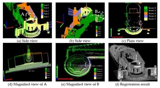
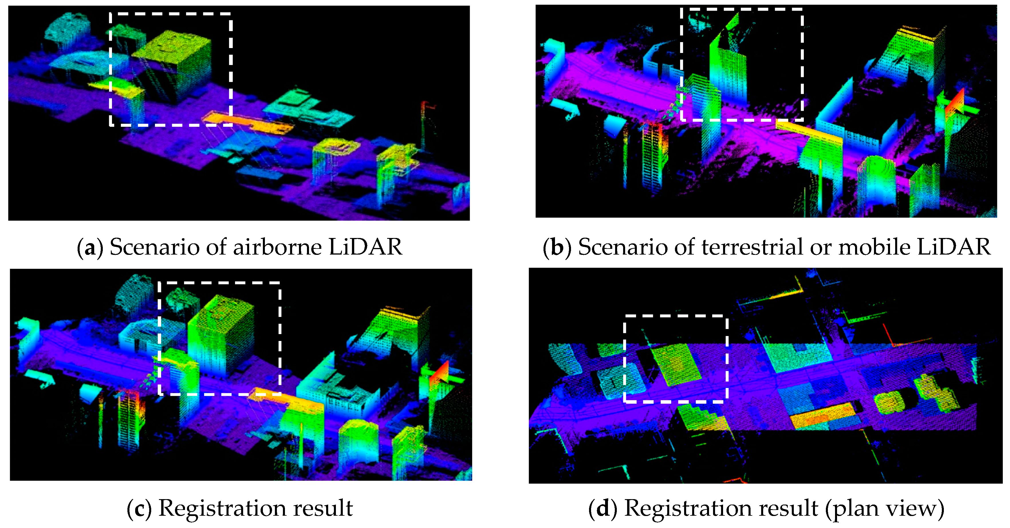
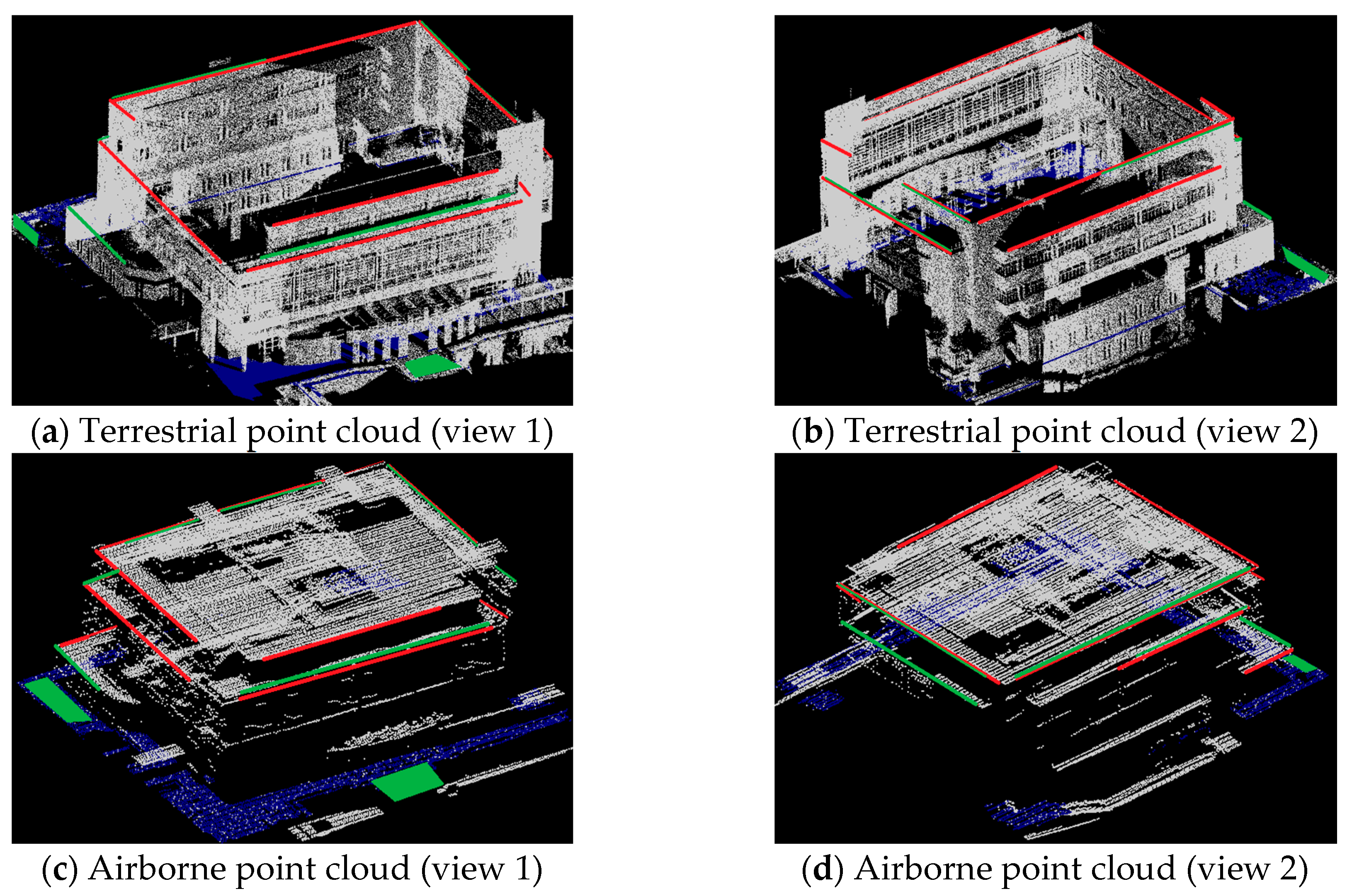
Light detection and ranging (LiDAR) has been an effective technique for obtaining dense and accurate 3-D point clouds. Related applications have emerged in many fields because of advances made in the evolutions of data acquisition and processing [1,2]. Different LiDAR platforms are designed to operate with different scanning distances, scanning rates, and scanning directions. Therefore, point clouds generated from different platforms may vary in density, accuracy, coordinate systems, and scenic extent. Airborne LiDAR system (ALS) renders point clouds covering explicit top appearance of objects (Figure 1a), while mobiles LiDAR system (MLS) and terrestrial LiDAR system (TLS) provide façades and object surfaces (Figure 1b). To make use of the complementary information and generate a complete dataset of 3-D scenes (Figure 1c,d), data integration of different platforms or scans is indispensable. Even if the global navigation satellite systems (GNSS) and inertial navigation systems (INS) are available to the ALS and MLS, problems caused by position and orientation system, mounting errors, and shadowed effect warrant a rectification step for quality products. Thus, registration can be regarded as a pretreatment in terrestrial LiDAR data processing to transfer point clouds collected from different scans onto a suitable reference coordinate system, and also utilized as a refinement procedure to adjust small misalignments either between adjacent strips of airborne or neighboring mobile LiDAR data or between the data collected through two different platforms. A proper registration methodology, being able to tackle the inconsistency between different point clouds, appears crucial to numerous point cloud applications.
Indeed, considerable solutions for point cloud registration have been proposed in the literature. Existing methods can be classified into several types, in which surface- and feature-based approaches are commonly employed and yield high-quality results. The iterative closest point (ICP) algorithm developed by [3,4] is the most commonly used surface-based algorithm. Many follow-up improvements [5,6,7,8] have promoted ICP efficiency. In addition, other related studies, such as the iterative closest patch [9], the iterative closest projected point [10], and the least-squares surface matching method (LS3D) [11,12], have also proven their effectiveness in point cloud registration. On the other hand, numerous feature-based techniques have been developed based on geometric primitives, such as points, lines [13,14,15,16], planes [13,17,18,19,20], curves and surface [21], and specific objects [22]. Methods manipulating image techniques for laser scans [23,24,25,26], and refining the 3D fusion based on the correlation of orthographic depth maps [27] have also been studied for registration purposes. Wu et al. [28] employed points, lines, and planes to register lunar topographic models obtained by using different sensors. Han [29] and Han and Jaw [30] applied hybrid geometric features to solve a 3-D similarity transformation between two reference frames. An extended work of Chuang and Jaw [31] aimed at finding multiple feature correspondences with a side effect of sequentially gaining 3-D transformation parameters, facilitating the level of automatic data processing. Furthermore, the ideas of 2D feature descriptors, such as scale-invariant feature transform (SIFT) [32], smallest univalue segment assimilating nucleus (SUSAN) [33], and Harris [34] operators, were also extended as Thrift [35] and Harris 3D [36] to work with 3-D fusion and similarity search applications [37,38,39,40,41,42], but the current studies mostly undertook the evaluation of shape retrieval [43] or 3D object recognition [44] using techniques such as the shape histograms [45], scale-space signature vector descriptor [46], and local surface descriptors based on salient features [47].
Studies with a focus on cross-based registration can be found as in [15,48] which registered terrestrial and airborne LiDAR data based on line features and combinations of line and plane features extracted from buildings, respectively. Teo and Huang [49] and Cheng et al. [50] proposed a surface-based and a point-based registration, respectively, for airborne and ground-based datasets. However, the inadequate overlapping area of the point clouds of the ALS and MLS or TLS as the scenarios demonstrated in Figure 1a,b raises challenges for acquiring sufficient conjugate features and thus is apt to result in unqualified transformation estimation. In addition, the majority of post-processing methods perform pair-wise registration rather than simultaneous registration for consecutive scans, and the uncertainty of related observations has rarely been considered during the transformation estimation. The registration errors tend to accumulate as running each pair transformation sequentially. On the other hand, the ignorance of varying levels of feature observations errors would lead to the bias of the estimation.
It also drew our attention to the fact that the existing studies of feature-based point cloud registration employing line and plane features either utilized only partial geometric information [13,28] or needed to derive necessary geometric components with alternative ways [29,30]. In this study, we focused on the employment of features versatile in types as well as both complete and straightforward in geometric trajectory and quality information. The main contribution of this paper is the rigorous mathematical and statistical models of the multi-feature transformation capable of carrying out global registration for point cloud registration purposes. Considering the point, line, and plane features, the transformation model was driven by the existing models to improve the exploitation of features on both geometric and weighting aspects and to offer a simultaneous adjustment for global point cloud registration. Each type of feature can be exclusively used or combined with the others to resolve the 3-D similarity transformation. Since the multiple features with full geometric constraints are exploited, a better quality of geometric network is more likely to be achieved. To correctly evaluate the random effect of feature observations derived from the different quality of point cloud data, the variance–covariance matrix of the observations is considered based on the fidelity of data sources. Thus, the transformation parameters among multiple datasets are simultaneously determined via a weighted least-squares adjustment.
The workflow of the multi-feature registration involves three steps comprising the feature extraction, feature matching, and transformation estimation. Although considerable researches on extracting point, line [51], and plane [49,52] features from point clouds have been reported, fully automated feature extraction is still a relevant research topic. We leveraged a rapid plane extraction [53] coupled with a line extractor [51] to acquire accurate and evenly-distributed features and then performed the multiple feature matching approach called RSTG [31] to confirm the conjugate features and to derive approximations for the nonlinear transformation estimation model. Nevertheless, the authors placed a focus on transformation estimation modeling and left aside the feature extraction and feature matching with a brief address referred to the existing literature. Two equivalent formulae for line and plane features, respectively, using different parametric presentation were proposed in the transformation model. The detailed methodology of how the transformation models were established and implemented is given in the following paragraph. The terms “point feature” stands for “corner or point-like feature”, while “line feature” employs only straight line feature throughout the paragraphs that follow.
2. Concepts and Methodology
The proposed multi-feature transformation model integrates point-, line-, and plane-based 3-D similarity transformations to tackle various LiDAR point cloud registrations. Seven parameters, including one scale parameter (s), three elements of a translation vector (, and three angular elements of rotation matrix , are considered for the transformation of scan pairs. The feasible parametric forms of observations used in this paper are the coordinates of points (), two endpoints () as well as six-parameter () or four-parameter ) forms of lines, and two parametric forms of planes ( and ). The different parametric forms for the same type of feature were proposed to fit to the need of feature collection or measurement. In fact, they are mathematically equivalent. Note that the geometric uncertainty, namely the variance–covariance matrix, of these feature observations has been integrated into the transformation estimation in this study.
2.1. Transformation Models
At the methodological level, the spatial transformation of point clouds can be established by the correspondence between conjugate points, the co-trajectory relation of conjugate lines, or conjugate planes. Equation (1) presents the Helmert transformation formula for two datasets on a point-to-point correspondence. To balance the transformation equation for solving seven parameters while providing a sufficient geometric configuration, at least three non-collinear corresponding point pairs are required for a non-singular solution. Furthermore, Equation (1) is employed to derive line- and plane-based transformations in the following paragraphs.
with
where s is the scale parameter; is translation vector; is a rotation matrix; and ω, φ and κ are the sequential rotation angles. and () represent the coordinates of the ith conjugate point in systems 1 and 2, respectively.
2.1.1. Transformation for Line Features
Two types of 3-D line expressions commonly employed in data acquisition were considered. The transformation model for the two-endpoint type of the line features (Figure 2a) is established by collinear endpoints of the line features with their conjugate counterparts when transformed to another coordinate system. The collinearity property for one endpoint may present three alternative forms, one of which is formulized in Equation (2).
where denotes the ith line; ; shows the transformed jth endpoint by Equation (1) from coordinate system 1 to system 2; for , either endpoint of represents the reference point of the ith conjugate line in coordinate system 2; and , derived by subtracting the corresponding coordinate component of the first end-point from the second one, represents the dicovt of the ith line in coordinate system 2.
As revealed in Equation (2), one pair of 3-D line correspondences contributes four equations (two for each endpoint) to the transformation. Similar to the two-endpoint model, the condition for the transformation model based on four-parameter line features can be established by constraining the direction vector and penetration point (which is determined by selecting the X–Y, Y–Z, or X–Z plane, called penetration plane, that supports the best intersection for the 3-D line) of the 3-D line to attain collinearity with their conjugate correspondents when transformed to another coordinate system (Figure 2b).
The right-hand side of Equation (3) shows the four independent parameters of the 3-D line when choosing X-Y intersection plane and they can also be derived from the six-parameter set. The mathematical formula of transformation based on four-parameter lines can be established in Equation (4).
where and represent the reference point and direction vector of the ith line, respectively; is the penetration point on the X–Y plane; is the reductive direction vector; and and are the scaling variables.
where denotes the transformed reference point (six-parameter type) or penetration point of the ith line by Equation (1) from coordinate system 1 to system 2; is the reference point or penetration point of the ith conjugate line in coordinate system 2; and represents the transformed direction vector of the ith line by Equation (5) from coordinate system 1 to system 2.
The six positional variables in Equation (4) may vary with the different penetration planes. Moreover, the conjugate lines from different coordinate systems may have varied penetration planes. Table 1 shows the appropriate use of parameters according to the facing condition.
The dual representation forms of the line-based transformation model given in Equations (2) and (4) are mathematically equivalent and suggest that one pair of conjugate lines offer four equations. At least two non-coplanar conjugate 3-D line pairs must be used to solve the transformation parameters. Furthermore, the line trajectory correspondence underpinning the 3-D line transformation allows flexible manipulation of feature measurements compared with the point-to-point approach.
2.1.2. Transformation for Plane Features
With the similar manipulation mentioned in the line-based model, two equivalent formulae using three independent parameters for plane-based transformation model were formed. A plane can be formulated in a normal vector form by considering the dot product of the normal vector and the point vector of the plane as one (Equation (6)) (zero if the plane includes the origin), or it can be formulated in a polar form by utilizing horizontal angle () and zenith angle () along with the projection distance () from the origin (Equation (8)). Notice that the normal vector employed in Equation (6) is the normalized normal vector of the plane divided by the projection distance. The transformation models are expressed in Equations (7) and (9) and both forms are depicted in Figure 3.
where denotes the ith plane; and and stand for the normal vectors of the ith conjugate plane in coordinate systems 1 and 2, respectively.
with
where () and () represent the parameter sets of the ith conjugate planes in coordinate systems 1 and 2, respectively. In fact, with , Equations (7) and (9) are mathematically equivalent.
2.2. Contributions of Features toward the Transformation Model
The characteristics of geometric constraints provided by these three types of observations vary from one type to another. A single point only contributes to translational (or locative) information, whereas unknown rotation and scale must be solved by points that span the area of interest. By contrast, a line feature provides the co-trajectory constraint along the line. This feature leaves the degrees of freedom of one scale, one translation, and one rotation parameter. A plane feature results in singularities in one scale, one rotation, and two translation parameters on the plane. Thus, line-based and plane-based approaches require features that supply complementary constraints for an entire solution. The application of different primitives is extremely appealing for the support of effective geometric constraints and can resolve situations that are considered difficult when the traditional point-based approaches are used.
Table 2 summarizes the transformation modes for the three primitives, where the numbers of independent pair correspondences for points, lines, and planes are notated by , , and , respectively, and is the number of scans. The effective number of equations generated by each feature is identical to the number of independent parameters, i.e., three, four, and three for a pair correspondence of point, line, and plane, respectively. The third column in Table 2 shows that the line features outperform the others in terms of redundancy.
When dealing with two scans, three point feature pairs with nine equations or two non-coplanar line feature pairs with eight equations are able to solve seven parameters of transformation. Nevertheless, according to Equations (7) and (9), it simply states that one conjugate plane pair will produce three equations which convey all the transformation parameters. However, four pairs of independent and well-distributed conjugate planes are the minimum requirements to solve seven parameters because planes, even if spatially isolated, may not be so complementary as an effective response to the transformation parameters. This statement can be understood by considering that three planes mutually perpendicular to each other contain only the information of three translation elements and three rotation angles even they supply nine equations. The scale factor cannot be fixed until a fourth plane is added.
Moreover, the intersected feature may gain geometric significance together with good quality of positional location at the expense of failing to completely represent the geometric property of the original data used for the intersection. An obvious example is that a corner point resulting from intersecting three neighboring planes brings forth only three equations for transformation, whereas these three planes are able to solve six parameters of 3-D rigid-body transformation. Besides the distinctive geometric characters elaborated by the individual primitive, appreciating the feature combinations realized by one point + one line, one point + two planes, one line + two planes, or two points + one plane in a minimum solution for seven-parameter similarity transformation of two scans is practically meaningful. Such configurations are arranged and analyzed in the experiments.
2.3. Simultaneous Adjustment Model for Global Registration
As mentioned before, the registration process for multiple scans often follows a pair-wise approach and then combines all results for the entire datasets. Consequently, registration errors between neighboring point clouds would gradually accumulate and result in a larger impact on those data distant from the reference one. In contrast, a global adjustment approach that simultaneously addresses the registration of all involved scans would minimize errors among all datasets. In such a simultaneously global registration manner, each feature observation in a scan is associated with only one residual, instead of receiving a residual as it is conducted by passing the pairs if the feature appears in more than two scans.
The Gauss–Helmert model of the least-squares adjustment is used to cope with diversified uncertainty treatment of registration tasks. Equation (10) expresses the mathematical form of the simultaneous adjustment model. Once a data frame is chosen as the reference, all other frames are co-registered by conducting the multi-feature transformation.
with
where Equations (2) and (7) are used for line and plane features in this formula. , , , and denote the observation vector, error vector, discrepancy vector, and incremental transformation parameter vector, respectively; is the weight matrix; and are the partial derivative coefficient matrices with respect to unknown parameters and observations, respectively; is the variance component; , , and are the numbers of total matched mates of points, lines, and planes, respectively; , , and represent the numbers of the conjugate features of ith matched mate; 6 based on Equation (2), otherwise 4 based on Equation (4); and is the number of all scans. On the other hand, if Equations (4) and (9) are employed, the and in matrices and should be replaced with and , and the and are replaced with and , respectively.
According to the Equation (10), the convergent least-squares solutions of the estimated parameter vector , residual vector , posterior variance component , and posterior variance–covariance matrix of the estimated parameter can be computed through Equations (11) to (14), where represents the redundancy.
with
The uncertainty of the observations, resulting from feature extraction, is considered and propagated based on how the feature parameters, namely the parametric forms as previously introduced, are acquired to form the variance–covariance matrix of the observed features. The indicates the covariance between two different feature observations if needed. The quantities revealed in the variance–covariance matrix present the feature quality that often results from the measuring errors and discrepancy between the real scene and the hypothesized scene. Basing the observation uncertainty on the fidelity of the data source is considered an optimal way of assessing and modeling weights in this work. The weight matrix , which is derived from the variance–covariance matrix of the observations, is then fed into the adjustment model.
3. Experiments and Analyses
The effectiveness of the registration quality provided by the individual and combined features was validated using the simulated data. The configurations of simulated data were designed to put more concerns on validating mathematical models in solving the transformation parameters with varied features, different levels of data errors, minimal and nearly minimal observations, thus rendered so ideal as well as fundamental as compared to the practical data that often involved much complicated scenes with feature distribution and quality demanding cautious treatment.
Real scenes with feature appearances collected by TLS, ALS and MLS that dealt with both single- and cross-platform registrations were subsequently demonstrated to reveal the feasibility and effectiveness of the proposed method. To fairly evaluate the merits of the proposed registration scheme in handling multiple scans, we compared our results with those obtained by the ICP algorithm initiated by Besl and McKay [3] and the line-based method [51]. These methods were coded in Matlab and realized on a Windows system.
The customary way of assessing transformation and registration quality is to utilize the root mean square error (RMSE) based on the check points with . Under the mode of multi-feature transformation, the positional discrepancies of the conjugate points, geometric relationships quantified by angles and distances for both conjugate lines and planes are considered as registration quality indicators. Apart from the RMSE criterion, a distance indicator in Equation (15), the average of the spatial distances of all the conjugate line segments and plane patches, is used to evaluate positional agreement. Similarly, an angular indicator in Equation (16), the average angle derived from all the conjugate line segments and plane patches, is used for evaluating geometric similarity.
where is the average distance of each middle point of the ith conjugate line segments to its line counterpart along the direction perpendicular to the line, and is the average distance of each centroid of the ith conjugate planes to its plane counterpart along the normal direction. and are the total numbers of independent conjugate line and plane pairs, respectively. is the angle of the th conjugate line pair computed by the direction vectors. is the angle of conjugate plane pair computed by the normal vectors.
The positional accuracy of each laser point is a function of range, scanning angles, and positioning/pose observations, if applicable. The proposed quality indicators reflect the registration accuracy upon the reference data. The point interval of a point cloud intimates the minimum discrepancy of the raw quality considering the discrete and blind data nature. Thus, we intuitively included the point spacing of the point cloud into quality analysis for the real datasets, particularly if it prevails over the point error. In addition to employing check features, we also introduced the registered features into Equation (15) to derive internal accuracy (IA), which has the same meaning as the mean square error (MSE) index of the ICP algorithm [3]. The index resulting from transformation adjustment would not only be used to assess the registration quality but also suggest whether the internal accuracy and the external one derived from check features are consistent.
3.1. Simulated Data and Evaluation
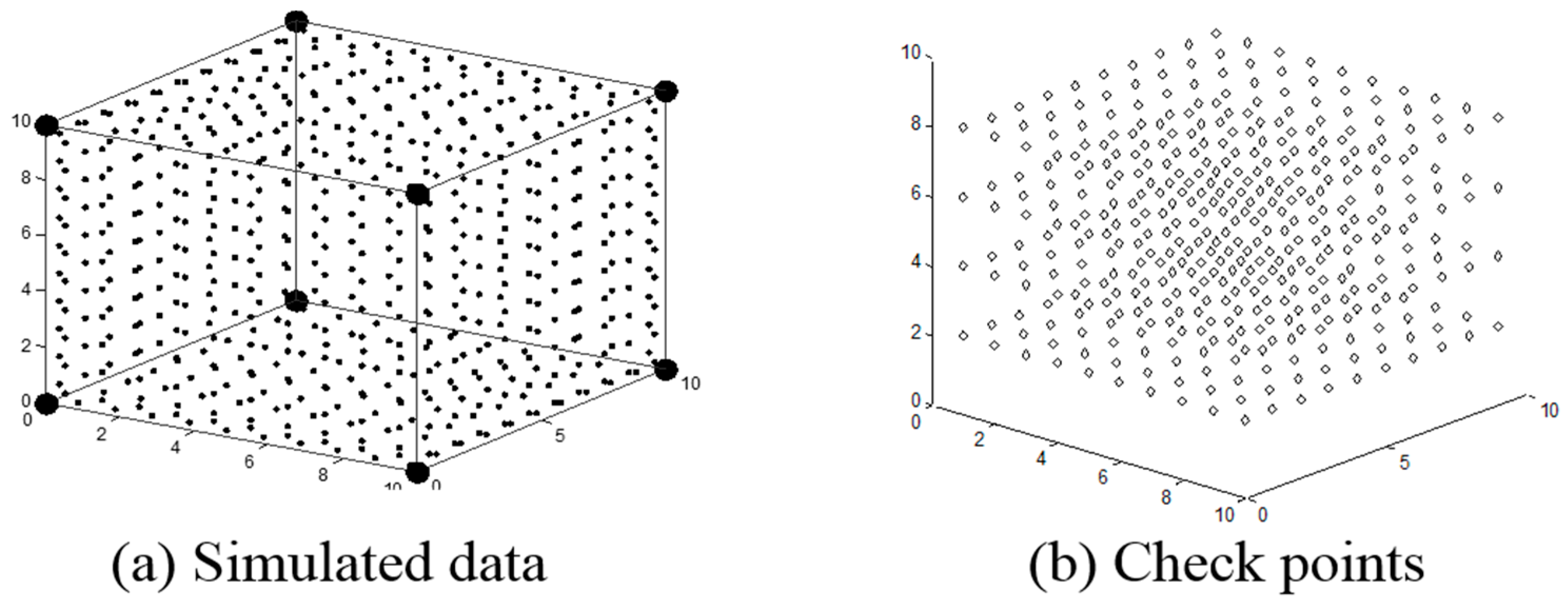
To simplify the scene geometry and concentrate on validating the mathematical models, simulated data with a size of approximately 10 m × 10 m × 10 m were generated in this experiment. Figure 4a shows a point cloud forming a cube, in which 6 planes, 12 lines, and 8 points can be extracted as observations. Four layers of check points, denoted as rhombuses in a total of 400 points, as shown in Figure 4b, were densely arranged and situated inside the cube for exclusively evaluating the registration quality. The point cloud was transformed using a pre-defined set of similarity transformation parameters to represent the data viewed from another station. To simulate the random errors of terrestrial scans, both the simulated and transformed point clouds were contaminated with a noise of zero mean and σ cm standard deviation, where σ ∈ {0.5, 1.5, 2.5, 3.5, 4.5} in each coordinate component. In this case, the points and lines directly measured from the point clouds were considered the coarse features as they (points and endpoints) were determined with the same positional quality as that of the original point. On the other hand, features extracted by fitting process or by intersecting neighboring fitted planes were deemed the fine observations with better accuracy than original point cloud.
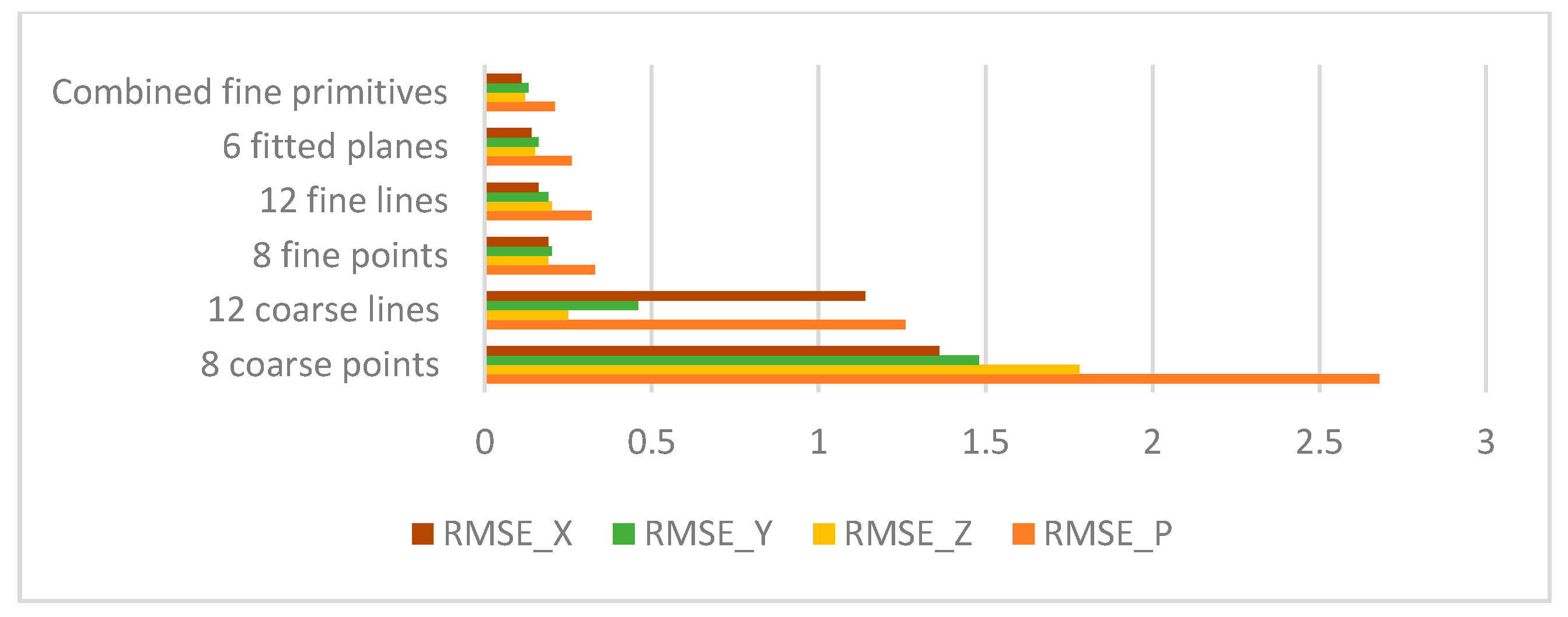
First, the influence of the coarse features versus fine features on the transformation quality was observed as well as the registration effectiveness derived from individually and unitedly as the observations when σ = 1.5 cm was added. This exhibited that transformation can be solved by either applying a single type of features or the combination of multiple features. Figure 5 reveals the registration quality. To assess the quality of estimated transformation parameters, the solved parameters were used to transform the 400 check points from one station to another and computed the RMSE_P.
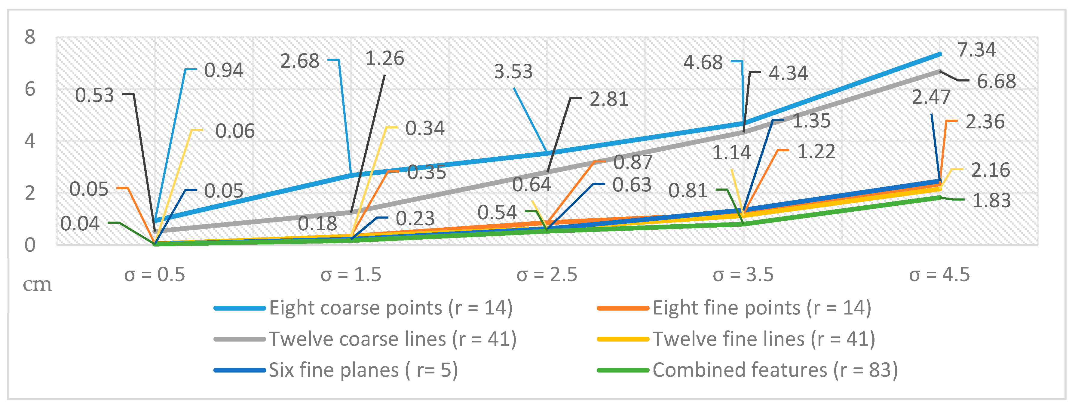
In light of Figure 5, applying fine features only in this case achieves registration quality ranging from 0.23 cm to 0.35 cm under the 1.5 cm standard deviation in each coordinate component of the point clouds, which is much better than the results of applying coarse features only, ranging from 1.26 to 2.68 cm. Using fine features even supplies transformation parameter estimation with sub-point accuracy of point clouds in this case. Obviously, combining all features also results in satisfactory registration quality. Further, to hypothesize the TLS data acquisition with reasonable error range, Figure 6 shows the RMSE_P obtained from each observation set when the standard deviation of the point clouds is set as σ ∈ {0.5 cm, 1.5 cm, 2.5 cm, 3.5 cm, 4.5 cm}, respectively. As anticipated, combining all types of fine features resulted in the best RMSE_P under each data quality. As the deviation increased, namely worsened observations, the advantage of the feature integration became more obvious. It can be seen in Figure 6 that the error trend of employing feature combination, benefiting from the accurate observations and high redundancy (83 in this case), grew moderately as compared to those utilizing single feature type.
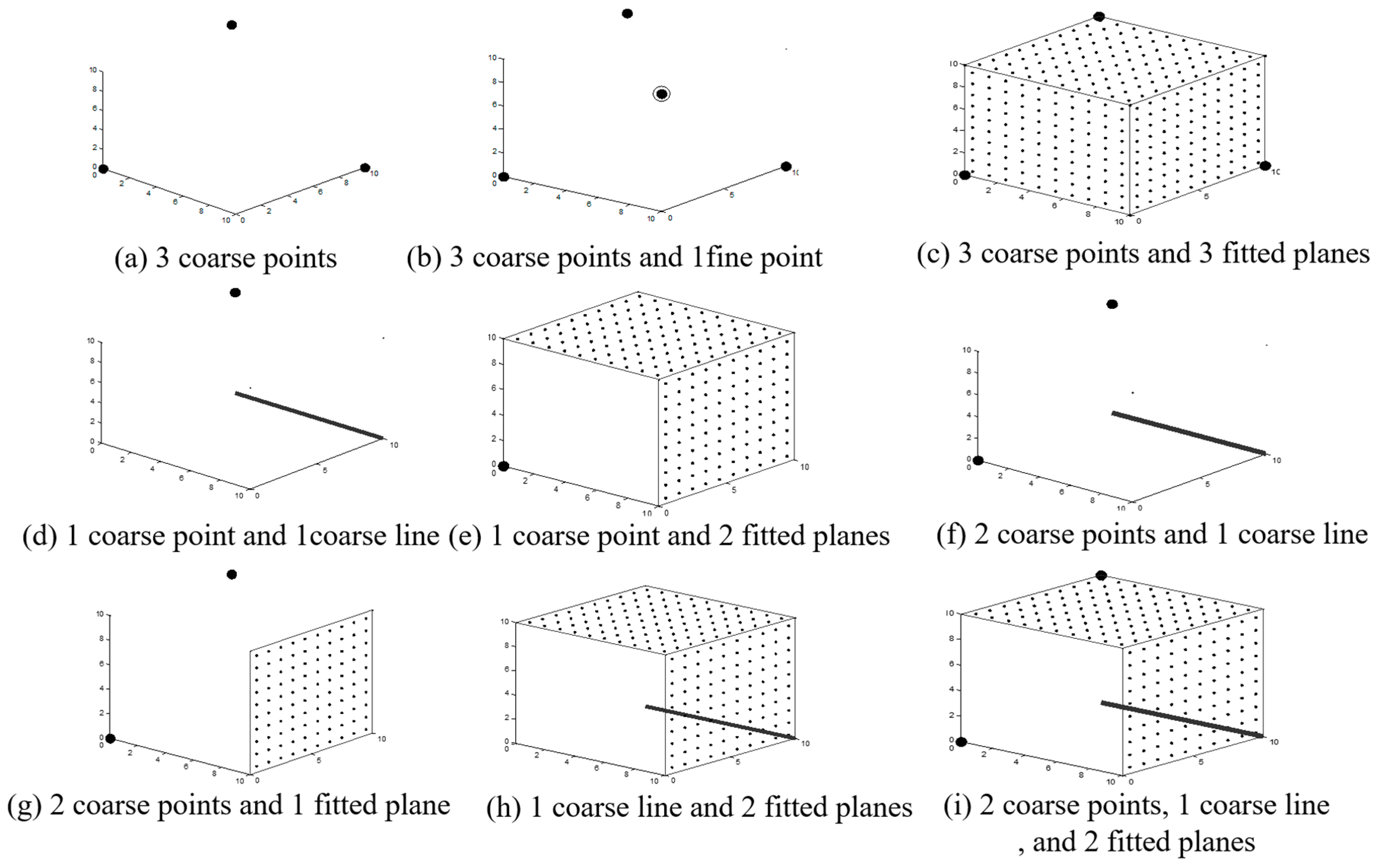
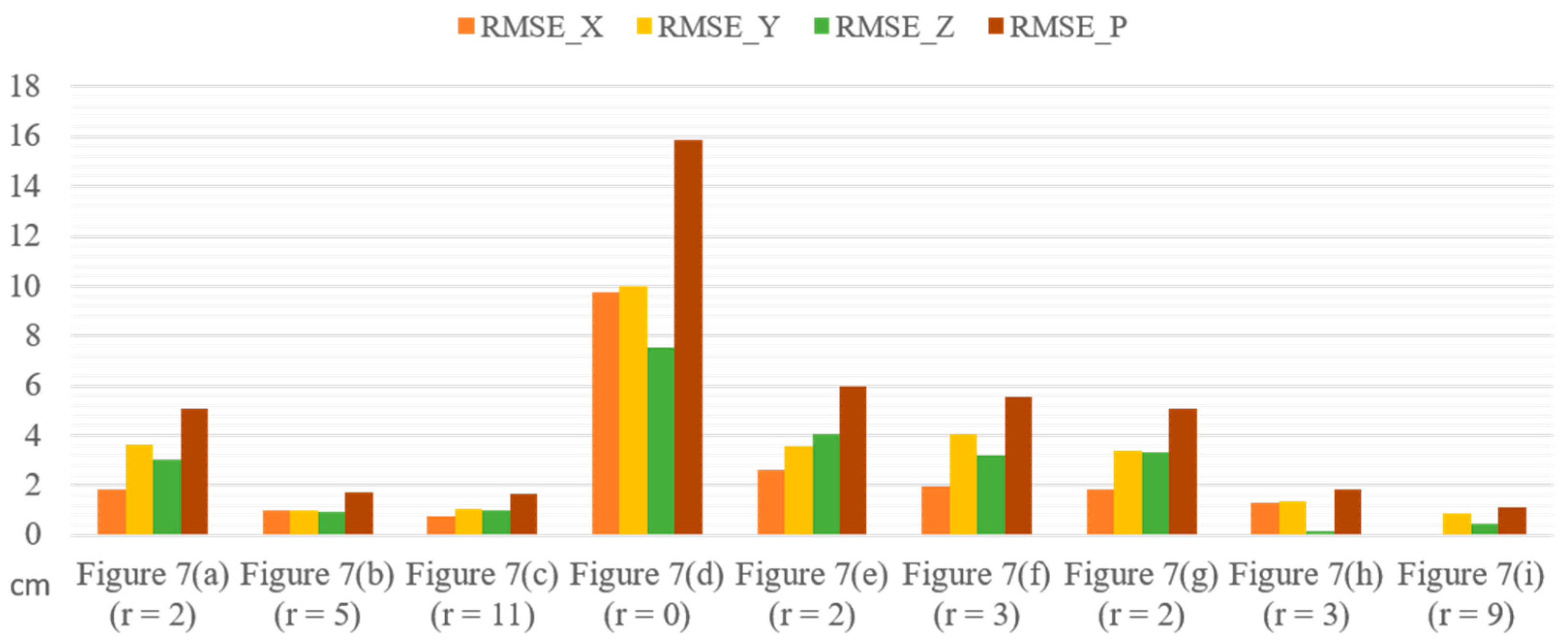
Further, nine minimal or nearly minimal configurations of observations for transformation estimation were investigated to show the complementariness among observed points, lines, and planes. The distribution of the features is illustrated in Figure 7a–i. Specifically, Figure 7a–c was designed to analyze the different benefits gained from an intersected point versus three planes that determined the point. Figure 7d–i was configured to verify the feasibility of multiple feature integration by laying out the feature combinations under the condition of only a few or nearly minimum measurements for estimating the transformation parameters. The evaluations of transformation quality in relation to all the cases are presented in Figure 8, where r indicates the redundancy.
Again, transformations in all nearly minimal solution configurations were resolved. From the comparison of transformation results of Figure 7b versus Figure 7c, both sharing the three coarse points as shown in Figure 7a, it showed that when the three fitted planes, deemed as fine features, were added, the transformation accuracy was slightly increased with a lower RMSE_P (0.07 cm) than adding the fine point intersected by these three planes. This effect gave a numerical example to further add to what was stated in Section 2.2. In the configurations of Figure 7d–h, the transformation estimations using the united features under the minimum measurement condition were demonstrated. It should be noted that the specified number of each feature was insufficient to solve the transformation alone in these cases. Considering the RMSE results in Figure 8, the combination of one point and one line (Figure 7d) resulted in dramatic transformation errors because of its poor distribution and zero redundancy. Transformation errors were reduced with better-distributed features, as those in Figure 7a,e–h. On the other hand, the configuration of Figure 7i which combined the well-situated two points, one line, and two planes, gained the best transformation quality among all the cases.
Considering points are relatively likely to be obstructed between scans than other features as well as the distribution of planes in urban scenes is often monotonous, combinations of these feature primitives would bring more adaptability to conquer distribution restrictions frequently confronted in practical cases. The simulated experiments demonstrated the flexibility of feature combinations and quantified the merits of solving the point cloud registration in a multi-feature manner.
3.2. Real LiDAR Data
To validate the advantage of the proposed registration scheme on real scenes, three cases consisting of the registration of terrestrial point clouds, the registration between terrestrial and airborne LiDAR point clouds, and the registration between mobile and airborne LiDAR point clouds were conducted. The first case demonstrated the routine terrestrial point cloud registration, while the second and third cases tackled the point clouds with different scanning directions, distances, point densities, accuracy, and having rare overlapping areas which is unfavorable for most surface-based approaches, e.g., ICP [3] or LS3D [11].
To evaluate the effectiveness of the registration quality, the registration results were compared with those derived from the ICP algorithm [3] and the line-based transformation model [51]. The comparison with the ICP highlighted the essential differences of the algorithm in terms of operational procedures (e.g., calculating strategy and with/without the need of manual intervention) and the adaptability for cross-based LiDAR platforms. On the other hand, the comparison with the line-based transformation was to illustrate the advantages of feature integration on the operational flexibility and accuracy improvement. Moreover, the last case demonstrated both the feasibility and working efficiency of the proposed method in an urban area with larger extent as compared to the other two cases. Notably, the experiments were performed on the point clouds without any data pre-processing including noise removal, downsampling, or interpolation.
3.2.1. Feature Extraction and Matching
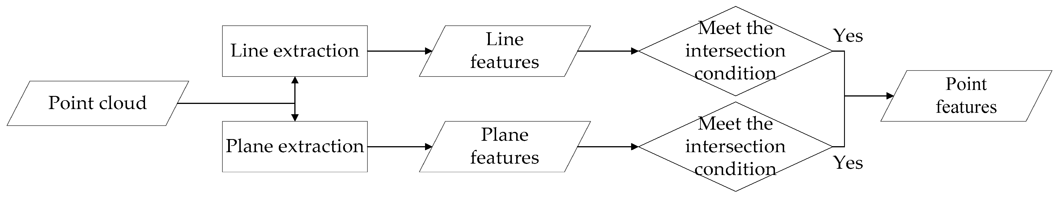
As fully automated point cloud extraction is still a developing research topic, the proposed registration scheme may couple with existing feature extraction approaches. From a standpoint of point cloud registration, to efficiently acquire qualified and well-distributed features is more important than acquiring complete features of the point cloud. In this study, we leveraged a rapid extractor [51,53] to acquire line and plane features and subsequently intersected neighboring lines or planes for points as long as an intersection condition is met [53]. Afterward, a 3D multiple feature matching approach [31] was implemented to obtain corresponding features and the approximations of similarity transformation between two data frames. The results were then introduced into the proposed model for rigorous transformation estimation. Figure 9 shows the workflow of feature acquisition in this study.
Conceptually, the extractor conducted a coarse-to-fine strategy to increase working efficiency. The point clouds were first converted into a range image and a 2.5-D grid data with a reasonable grid size according to the data volume, and the correspondence of coordinates was preserved. Although the process deteriorated the quality of the original data, the computational complexity was reduced. For line features, Canny edge detection and Hough transformation were implemented in the range image for detecting straight image lines. The image coordinates of line endpoints were then referred back to the original point cloud and used to collect candidate points for 3-D line fitting. On the other hand, the normal vectors of each 2.5-D grid cell were computed and clustered to find the main directions of planes in the point cloud. The information was introduced to the plane Hough transformation as constraints to reduce the searching space, so the computational burden for the plane extraction can be eased. Subsequently, lines or planes that met the intersection condition were used to generate point features [53]. Taking lines as an example, the extreme points within the group of points which described the line were first computed. Then, the extreme points of the line, being the endpoints, were used to compute the distances with the extreme points of other lines. If the shortest distance between the two lines was smaller than a tolerance (pre-defined by point space of data), the two lines were regarded as neighbors and used to intersect point feature. With the aid of this condition, virtual and unreliable intersected points, along with unnecessary calculations, were avoided. Besides, the quality measures of the resulting features were provided in the form of a variance–covariance matrix. Indeed, even though the coarse-to-fine procedure, which reveals approximate areas where features are possibly located and then aims at these areas to precisely extract the features from the raw point cloud, promotes the working efficiency and encourages the level of automation, the feature extraction is still the most computationally expensive step in this study.
Afterward, the extracted features were introduced to the multiple feature matching approach, called RSTG [31], to confirm the feature correspondence and to derive the initial values for the transformation estimation. The RSTG is the abbreviation of the matching approach which comprises four steps, namely rotation alignment, scale estimation, translation alignment, and geometric check. It applied a hypothesis-and-test process to retrieve the feature correspondence and to recover the Helmert transformation in an order of rotation, scale, then translation. The rotation matrix was determined by leveraging the vector geometry [29] and singular value decomposition, whereas the scale factor was calculated by a distance ratio between two coordinate systems. After that, the translation vector was derived from a line-based similarity transformation model [51] based on a collinearity constraint. The approach got rid of the point-to-point correspondence of the Helmert transformation, leading to a more flexible process. Details of the extraction and matching processes can be referred to [31,51,53].
3.2.2. Registration of Terrestrial Point Clouds
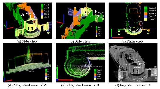
In this case, five successive scans, which cover a volume of 26 m (length) × 18 m (width) × 10 m (height), collected by Trimble (Mensi) GS200 describing the main gate of National Taiwan University in Taipei, Taiwan, were used. The nominal positional accuracy of 4 shots as reported by the Trimble manufacturer was up to 2.5 mm at 25 m range. The details of this dataset and the point clouds are shown in Table 3 and Figure 10, respectively.
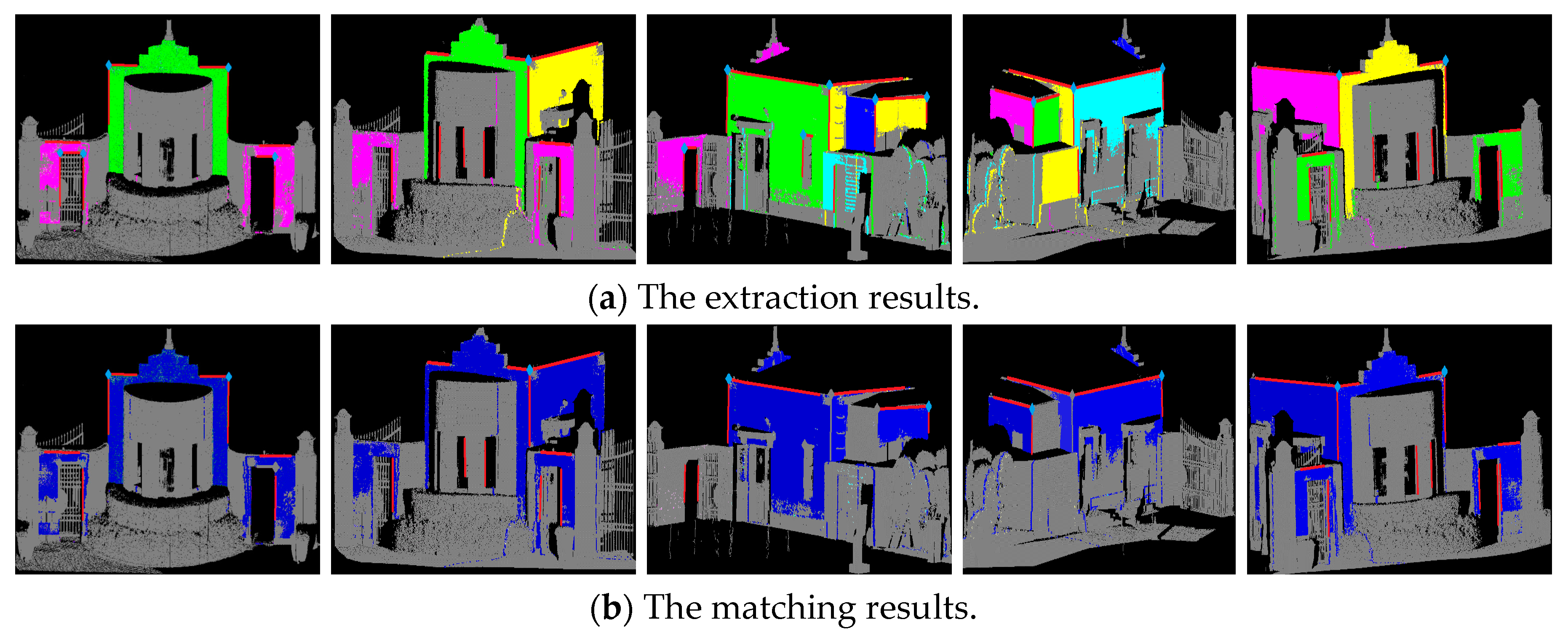
The number of acquired features in all scans was 95 features in total, consisting of 17 points, 57 lines, and 21 planes. They were passed on to the RSTG matcher. Figure 11a illustrates these features superimposed on the point clouds. The extracted lines were highlighted in red lines, the extracted points were marked in blue rhombuses, and the points belonging to the same plane were coded by the same color. Figure 11b shows the feature correspondences, where the corresponding planes are in blue.
The RSTG approach successfully matched three points, 17 lines, and seven planes among all overlapping scan pairs. The feature correspondences and the approximations of transformation parameters were delivered to the process of transformation estimation. The registration of the terrestrial LiDAR point clouds was performed by the proposed simultaneous adjustment model of the multi-feature transformation. In addition, the approximations were applied to the ICP algorithm and the line-based transformation. To evaluate the registration quality, there were 24 check points acquired by best-fit spherical markers as well as 18 check lines and six check planes measured evenly and manually serving as independent check features.
The overall quality of registration indicated in Table 4 revealed that the positional and distance discrepancies were about 1 cm, and the angle deviation was about 0.3 degrees. The positional discrepancy RMSE_P derived from check points was quite close to the distance discrepancy ( calculated by check lines and planes. The angle deviation also represented similar spatial discrepancy as the other two indicators when considering the employed line features within 3 m length. This suggested that these three quality indicators were effective and consistent.
In light of Table 3, the quality and density of the point cloud data were high. As a result, the three approaches yielded similar registration performances at the same quantitative level. Both the internal accuracy (IA) and the external accuracy derived from the check features reported satisfactory registration. The proposed multi-feature method slightly outperformed the baseline implementation of the ICP and line-based transformation methods based on the same configuration: the same initial values and one-time execution. It is well known that the ICP method has numerous variants which apply other techniques, such as limiting the maximum distance in the X, Y and Z directions or filtering points containing large residuals, to reduce the number of inadequacy points because points far from the data center do not contribute important information about the scene and some of them could even be considered as noise. The afore-mentioned process would trade between the points in the vertical and the horizontal surfaces to avoid a final misalignment if the point number of one of the surfaces greatly dominates the other. Indeed, the registration quality can be improved by adjusting parameters and executing the calculation repeatedly. However, our study was interested in comparing the fundamental methodologies without ad-hoc parameter tuning and repeated manual intervention to assess the feasibility and effectiveness of these algorithms.
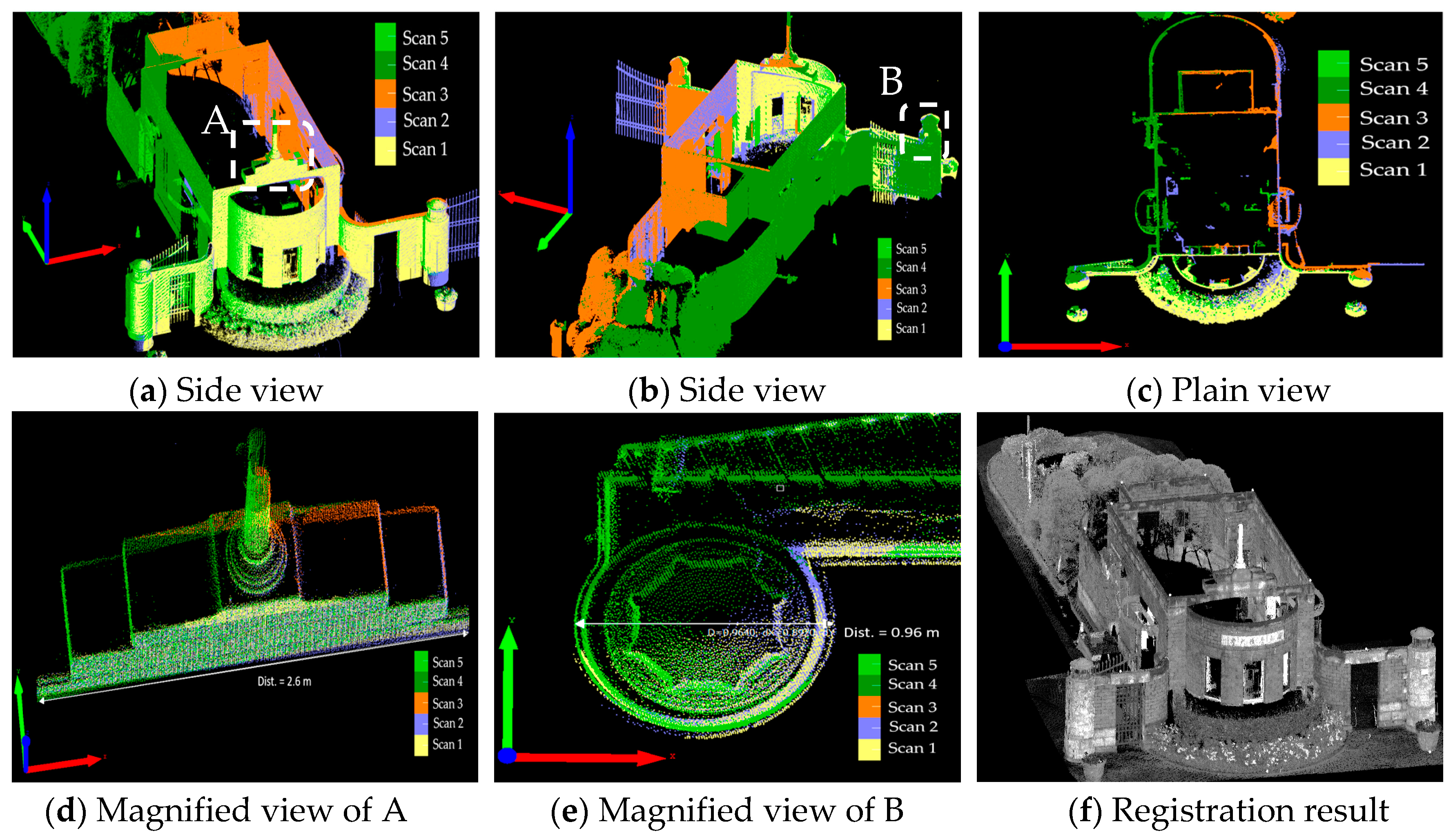
The results in Table 4 validated that integrating multiple features not only offered better operational flexibility, but also gained better registration quality than just exploiting line features. The visual inspections of the registration results of the proposed method can be found in Figure 12. The point clouds of each scan are drawn with different colors, where the discrepancy in overlapping areas is nearly undetectable and the facades collected by different scans are registered precisely.
The registration working process is nearly fully automated. In this case, the execution time for feature acquisition was about 3.24 min, and the matching and estimation process was about 41 and 2.7 s, respectively. The working time of the extraction and matching processes highly relates to the amount and complexity of point cloud data. Once the corresponding features are determined, the transformation estimation will be done in few seconds.
3.2.3. Registration of Terrestrial and Airborne Point Clouds
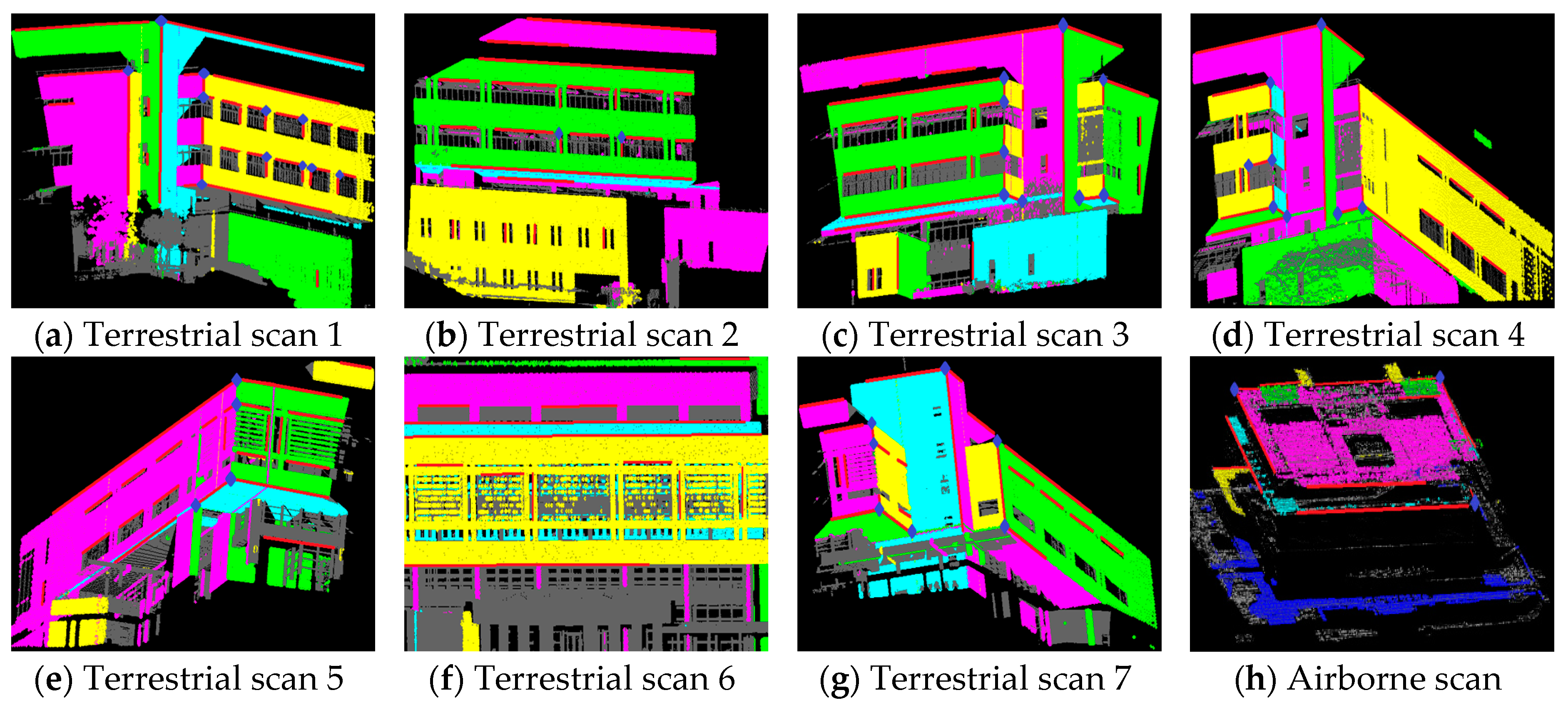
A complete scene of man-made structures that often appears in urban areas was considered in this case. A total of seven successive scans of terrestrial LiDAR point clouds were collected by the Optech ILRIS-3-D system. As displayed in Figure 13a–g, the scans cover the facades of a campus library building with a size of approximately 94 m (length) × 75 m (width) × 40 m (height). The nominal positional accuracy of a single shot for ILRIS-3-D is 8 mm at a range of 100 m. In addition, the airborne point cloud of the same building as shown in Figure 13h was collected via Optech ALTM 3070 at a flying height of 450 m with a reported elevation accuracy of up to 15 cm at a range of 1200 m and horizontal accuracy better than (1/2000) × flying height, which is approximately 23 cm in this case. Table 5 presents the information of all point clouds, in which scan 6 rendered the largest number of points and the highest density due to the large coverage of the target and the perpendicular scanning to the building facade.
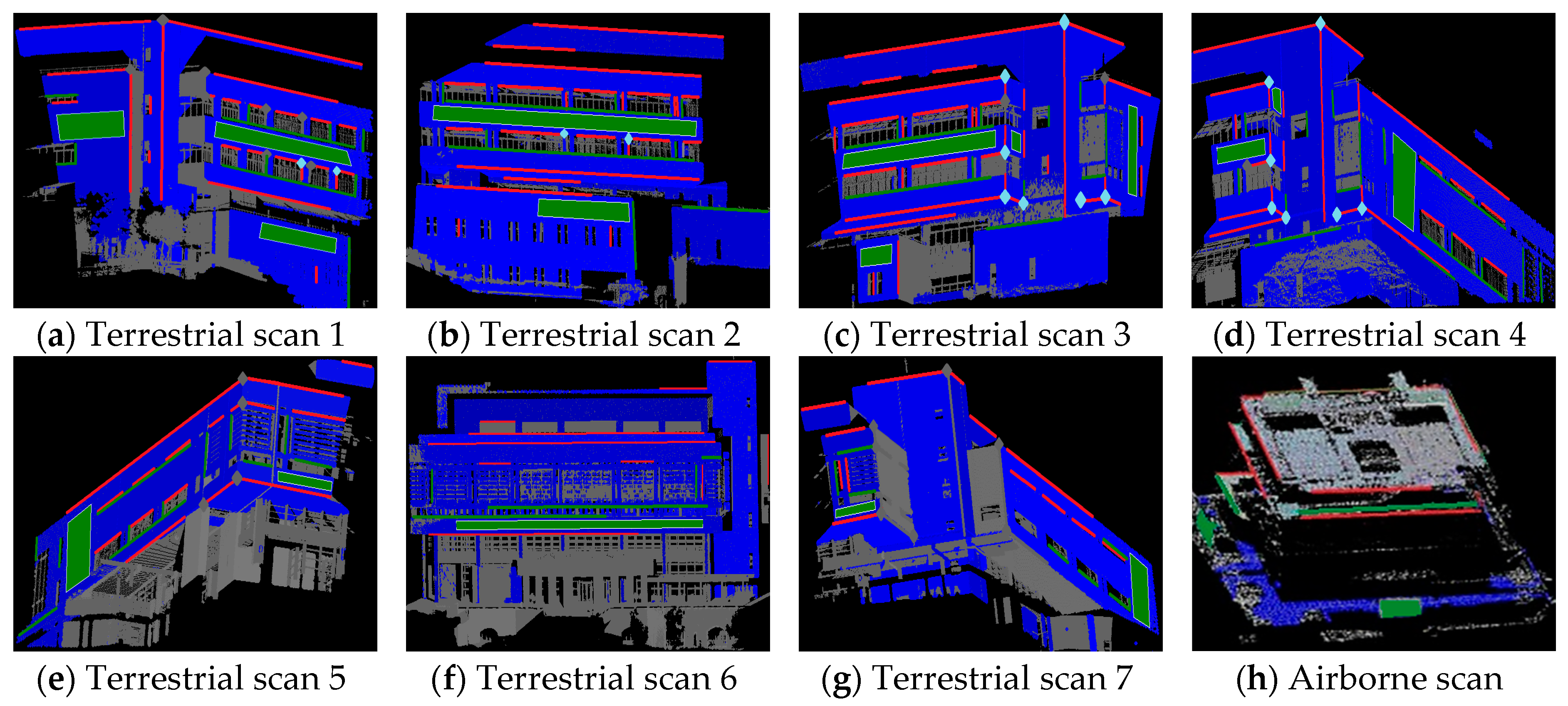
The extracted features were superimposed onto the point clouds, as illustrated by colors, following a similar coding as previous cases, in Figure 14. There were 297 well distributed features extracted within the scene. The numbers of extracted features are listed in Table 6.
As seen in Figure 15, each terrestrial scan rarely overlaps the airborne point cloud, and no single feature can fulfill the minimum requirement of the transformation estimation due to the poor overlap geometry in this case. Therefore, both the matching and transformation tasks were alternatively turned to process TLS first and then match and transform TLS to ALS. Again, the RSTG approach was applied to find the corresponding features of seven terrestrial scans and to render the approximations simultaneously. The successfully matched features among all overlapping scan pairs comprised nine points, 39 lines, and 15 planes, as shown in Figure 15a–g. The corresponding features were colored with the blue rhombus points, red lines, and blue planes, respectively. The correspondences along with the variance–covariance matrix of features and the approximations of transformation parameters were then introduced into the multi-feature transformation. However, the corresponding features between terrestrial scan 1 and scan 7 were not sufficient to construct stable transformation leading to an open-loop registration in this case. With the same basis of the initial transformation values, the ICP and line-based methods were performed to align all scans onto the reference frame (scan 6) accordingly.
Apart from the observed features, there were 20 lines and six planes, coded by green color in Figure 15, manually measured serving as independent check features to evaluate registration quality of the terrestrial registration. With the larger scanning distances and distance variations than the previous case, the significance of scale factor was studied in this case. Table 7 shows the estimated seven transformation parameters using the proposed simultaneous adjustment, whereas Table 8 reveals the six parameter results when the scale factor was fixed as 1. Further, the quantitative quality assessment of the terrestrial registration results is displayed in Table 9.
In the six-parameter case, the scale factor was fixed as 1, ignoring this effect as most rigid body-based methods would do. Considering Table 7, Table 8 and Table 9, the values of posterior variance , internal accuracy, , and report that taking the scale factor into account can obtain better registration results. The scale may bear certain systematic and random errors in this case, suggesting that solving seven parameters should render more comprehensive applications. However, the solved scale parameter needs also to be verified through significance test or based on prior information, if any, as not to accept a distorted solution. For example, the scale factor provided upon RSTG can be a very good approximation to be referred to. In Table 9, the proposed method yielded the best registration result, about 0.4 degrees in angle deviation and 1.6 cm in distance discrepancy, which is smaller than the average point spacing of the raw point clouds. Both the line-based and the proposed methods kept the consistency between the internal and external accuracy while the ICP did not. The MSE estimates resulted from each registration pair of the ICP nevertheless reached up to 3.3 cm, which indicated high internal consistency, even though the external accuracy was quite poor compared to either the proposed or line-based methods. This would suggest that the computation of the ICP might converge toward a local minimum. In addition, it could be understood that the ICP was affected by noise and its sequential pair-wise registration scheme made the cumulative errors grow significantly while dealing with open-loop scans.
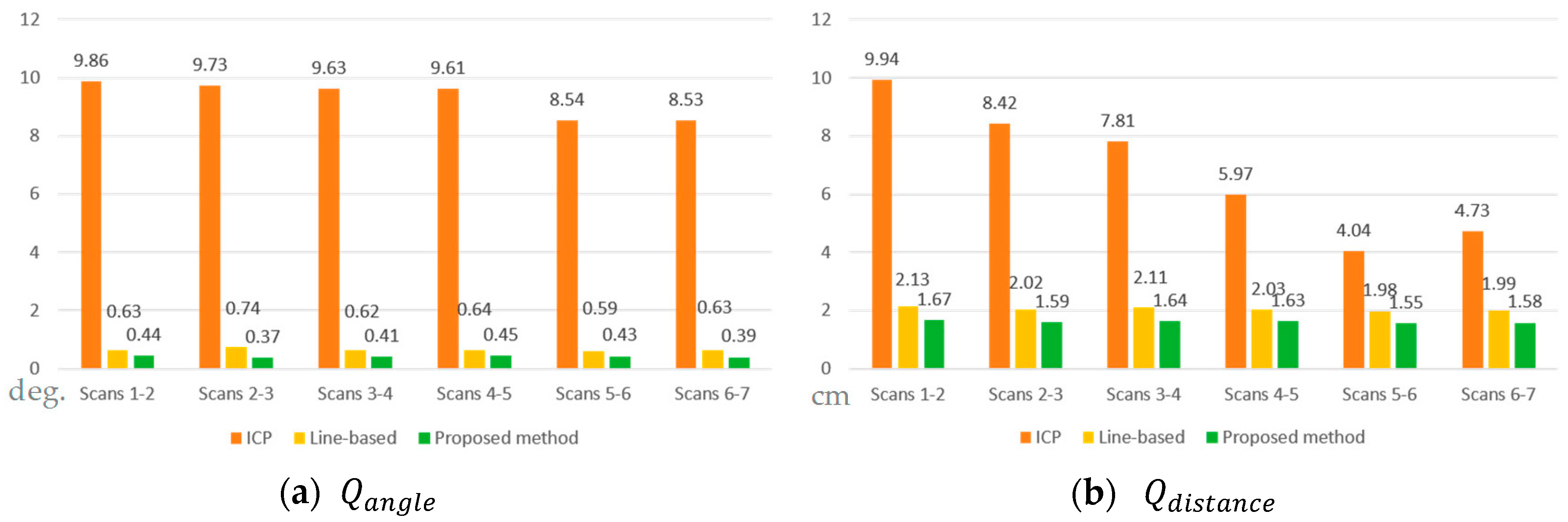
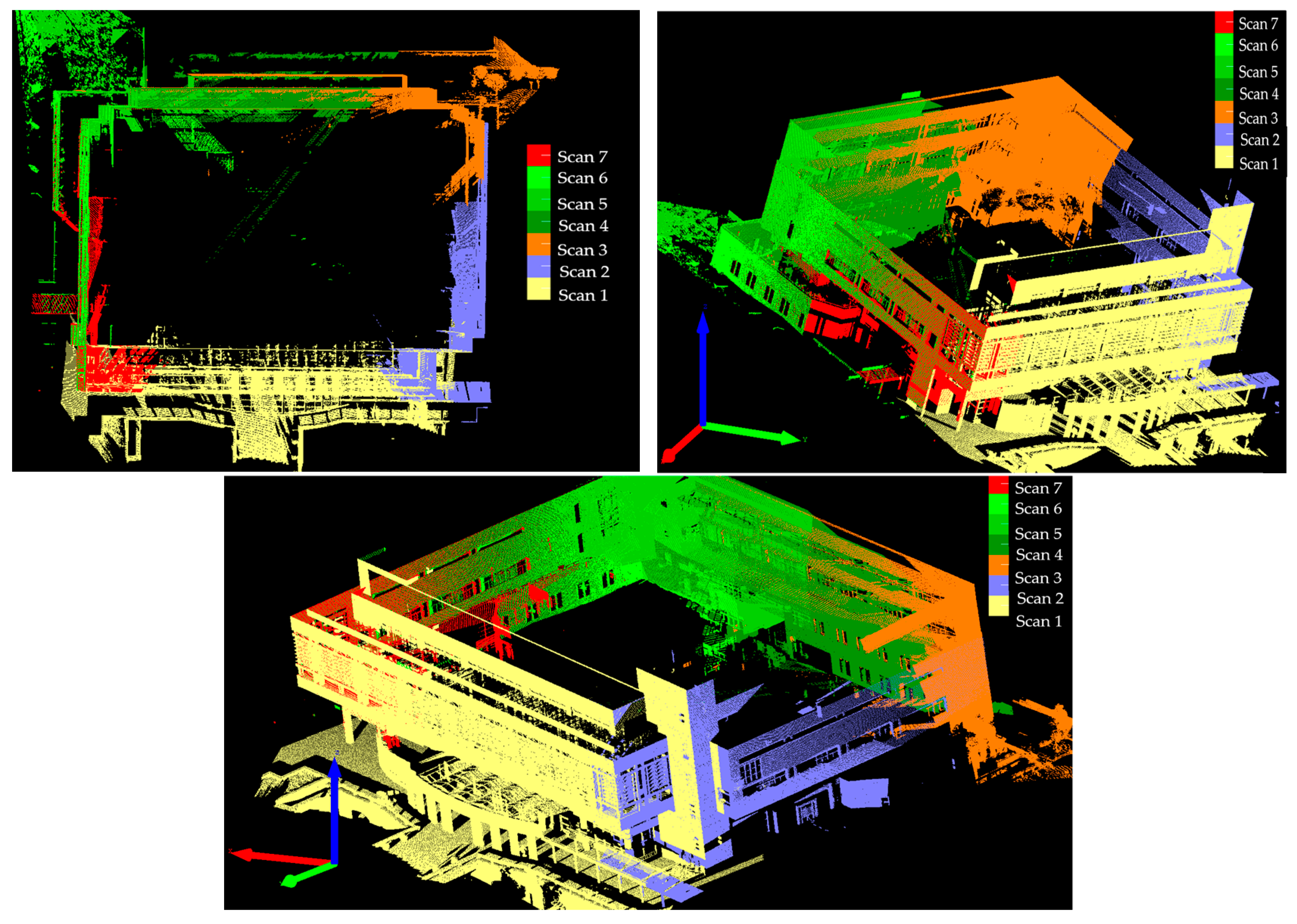
Figure 16 shows the distance and angular discrepancies at each scan pair. It reveals that the misalignment errors of the line-based and proposed methods were spread more uniformly among successive point clouds, while the discrepancies of the ICP were accumulated. Figure 17 illustrates the visual inspections of the registration result, where the point clouds of each scan are depicted in different colors. With the better feature distribution and redundancy (186 in this case), this terrestrial experiment highlighted the merits of the proposed simultaneous least-squares adjustment and the multiple feature integration in dealing with the global registration of successive scans.
After accomplishing the terrestrial registration, all features had been transformed onto the same coordinate system. Again, the RSTG approach was implemented to the terrestrial and airborne feature datasets for finding the conjugate features. There were nine lines and one plane correspondences found between the local coordinate and the global coordinate systems. It should be noted that the bulk of these data involved large geometric discrepancy raising the challenge of finding feature correspondences and the unavailability of reliable conjugate points. Nevertheless, it can be seen in Figure 15 that the normal vectors of plane features either in terrestrial or airborne scans are of less variation in geometric distribution. That is, most of the normal vectors of planes point to similar directions. It is intrinsically due to the specific scanning axis of LiDAR platform which would restrict the usage of surface-based approaches and plane features in cross-platform point cloud registration.
After feature extraction and matching, the TLS data were registered onto the ALS one by the three methods, and the registration quality was evaluated by 6 check lines and 1 check plane which were manually extracted from the point clouds. Figure 18 shows the matched features (red lines and blue plane) and check features (green).
As shown in Table 10, the check features point out that the registration quality of the proposed method is about 12 cm in distance discrepancy, slightly better than that of the line-based method. Apparently, considering the nature of the data characters, the dominant registered errors would inherit from the airborne point cloud. On the other hand, the ICP algorithm spoiled the registration in this case because the terrestrial and airborne datasets barely contained overlapping areas along the boundaries of the roof. The insufficient overlapping surfaces and the uneven data quality led the ICP method to converge to a local minimum. Indeed, the uneven data quality also directly affected the effectiveness of feature extraction and thus resulted in unequal accuracy of feature observations. The proposed multi-feature transformation did introduce variance–covariance matrices of observations into the adjustment process based on the fidelity of the data quality. If the uncertainty of features was not considered, namely unweighted, the registration quality deteriorated and the positional quality dropped almost 2 cm as compared to weighted result in this case. Therefore, by assigning appropriate weights and adjusting the feature observations accordingly would lead to the better transformation estimations.
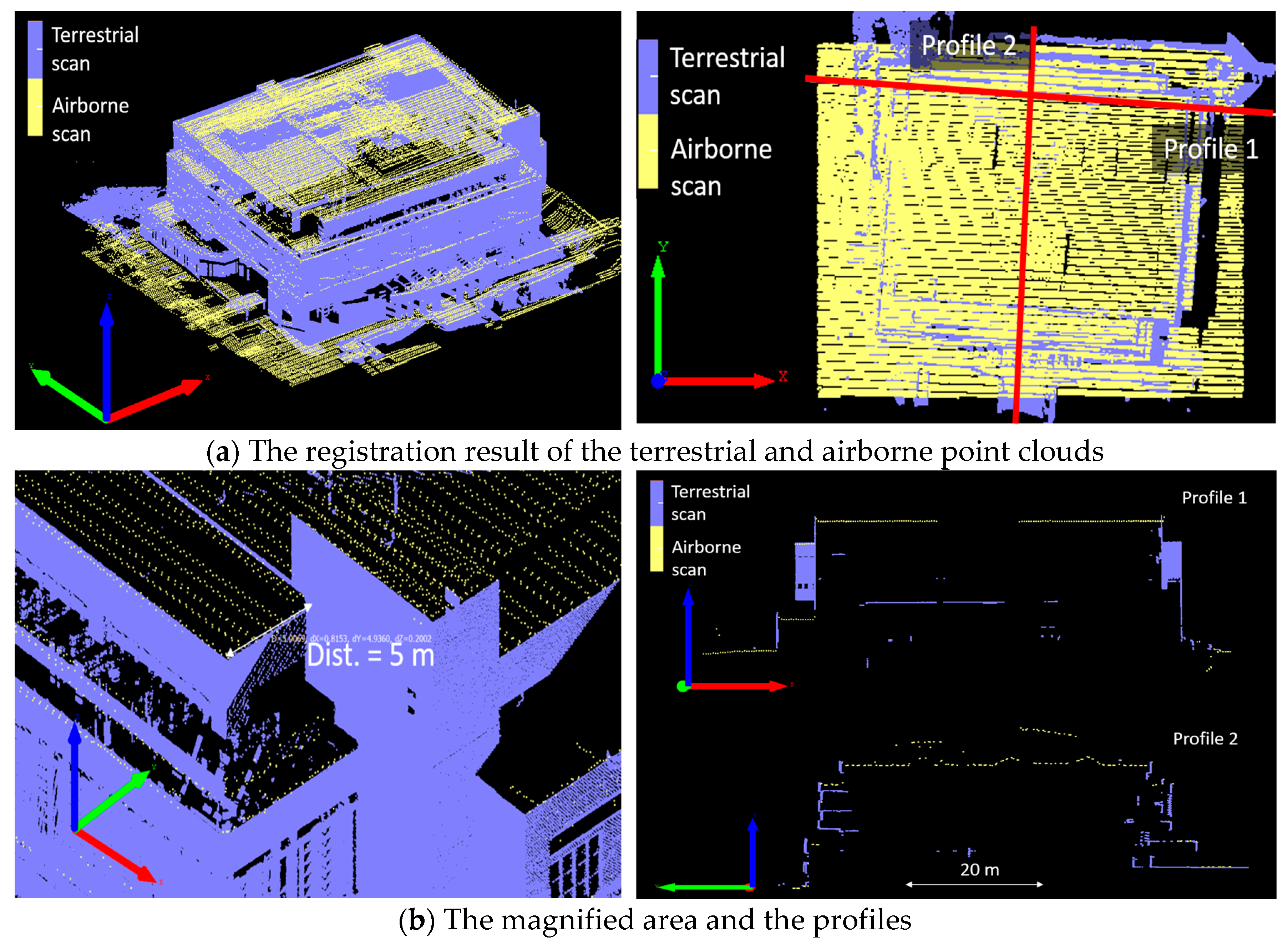
Figure 19 shows the visual inspections on the registered point clouds. It can be seen that the point spacing between airborne and terrestrial scans was extremely distinct. However, the junctions and the profiles in Figure 19b outlined the build boundary quite consistently. In addition, it is worth mentioning that the quantity of distance discrepancy listed in Table 10 is far less than the average point spacing (44 cm) of the airborne point cloud.
The registration between TLS and ALS manipulated only the line and plane features since the conjugate points were not available in this case. As a result, the internal accuracy of the line-based and the proposed methods appeared very similar but the external accuracy indicated that the proposed method was slightly better than the line-based method. The registration quality of line-based method may be influenced by the check plane which was away from the effective area of line observations. Even though line features were abundant, their reliability could be inferior to plane features considering their high uncertainty in the discontinuity area of point clouds [54]. Therefore, integrating multiple features into registration tasks would offer better solutions, especially for those scans rendering poor overlapping geometry. The total execution time of this case was about 4.5 min for feature extraction, 76.8 s for matching, and 2.4 s for transformation estimation.
3.2.4. Registration of Mobile and Airborne Point clouds
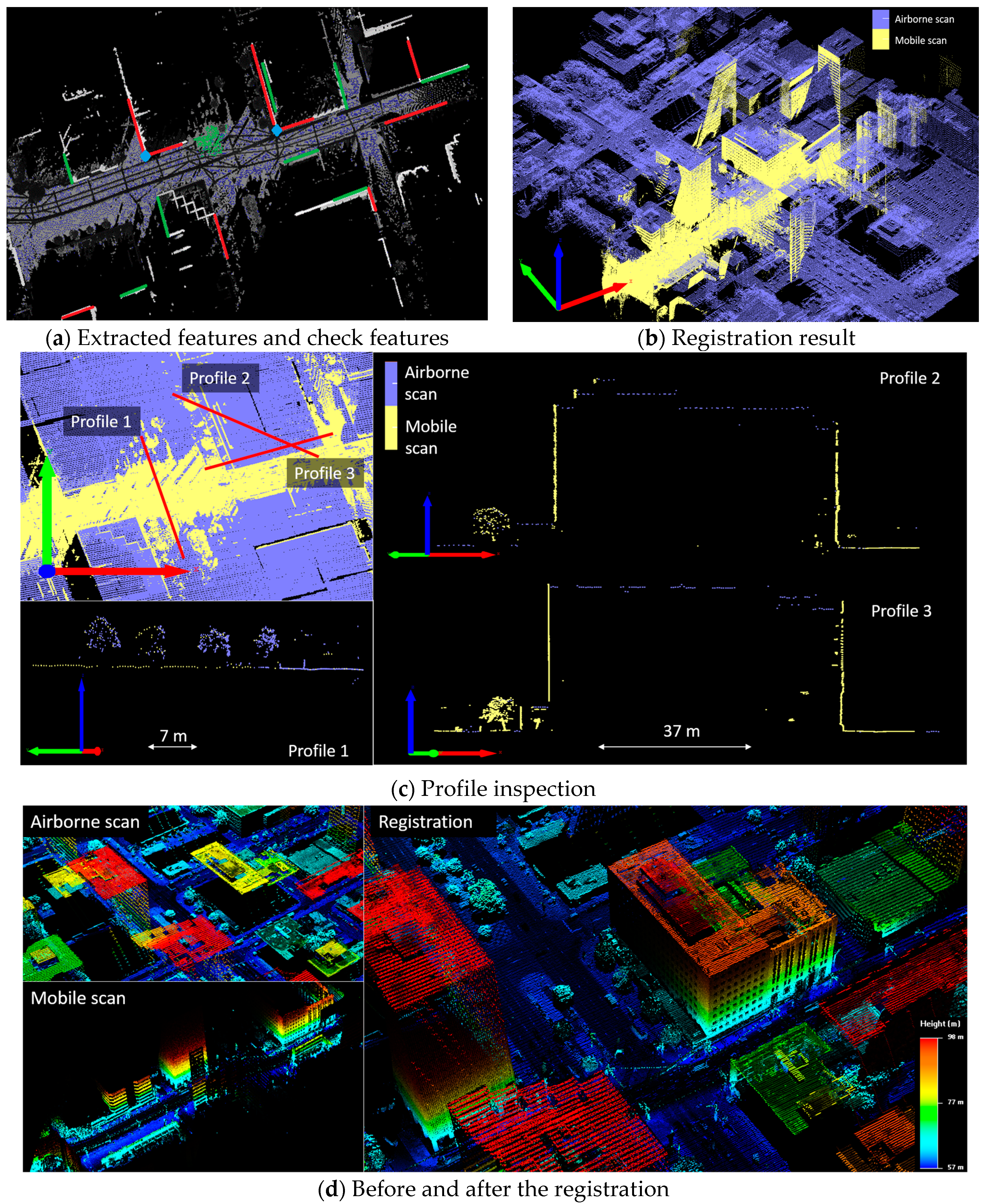
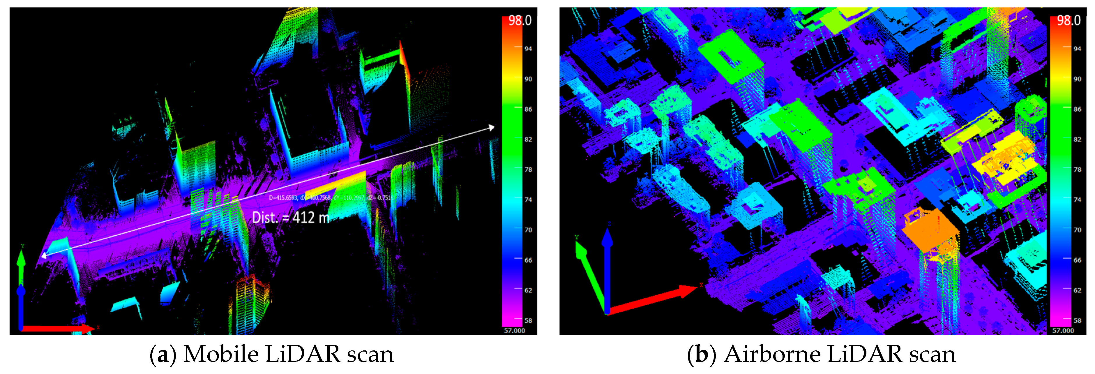
In this case, we applied the proposed method to the point cloud registration between mobile LiDAR system (MLS) and airborne LiDAR system (ALS). Regarding ALS and MLS, the exterior orientation of the sensor is typically known, so point cloud registration serves as a means of producing a best-fit surface through an adjustment process that compensates for small misalignments between adjacent data sets. Figure 20 shows the mobile and airborne scans of an urban area in Toronto, Canada. The mobile point clouds were collected utilizing Optech LYNX system. The absolute accuracy was 5 cm at 10 m range [55]. The airborne point cloud was collected by Optech ALTM 3100 at a flying height of 385 m with a reported elevation accuracy of up to 15 cm at a range of 1200 m [55] and approximately 19.2 cm horizontal accuracy in this case. The overlap area between the two data was about 412 m in length and 162 m in width, as shown in Figure 20a. The information of point clouds can be found in Table 11.
In order to reduce the computational complexity, we trimmed the airborne point cloud according to the mobile one and left the overlap area for feature extraction and matching. As illustrated in Figure 21a, there were two points, nine lines, and one plane retrieved from the overlap area, and even-distributed eight lines and one plane were manually collected as check features for quality assessment.
The quality indicators in Table 12 show that the remaining discrepancies are 8.7 cm in distance and 0.01 degrees in geometric similarity. Nevertheless, the visual registration result in Figure 21b demonstrates the detailed roof and façade of building structures, where the purple and the yellow points represented the airborne LiDAR and mobile LDAR data, respectively.
Apart from the quantity evaluation, three profiles (Figure 21c) were selected to visually inspect the junctions between MLS and ALS after registration. Profile 1 displayed the road point cloud and showed the consistency in plain area; and Profiles 2 and 3 demonstrated the roof and façade of the same building in two directions. The geometric agreement appeared not only on solid structure objects, but also on the tree-crown. Figure 21d exhibits the integrated point cloud result colored by height, which benefits further geometric exploration. The feature extraction process took about 7.5 min since the space extent of this point cloud data was larger than previous cases. The operation time for the feature matching and transformation was around 3.12 s.
4. Conclusions and Further Work
In this paper, the authors presented a multi-feature transformation model, exploiting the full geometric properties and random information of points, lines, and planes, for the registration of LiDAR point clouds. Simulated and real datasets were used to validate the robustness and effectiveness of the proposed method. The essential behavior of individual features through coarse versus fine measurements, single type of feature versus combined features, different levels of point cloud errors, and minimal and nearly minimal configuration of combined features applicable to the transformation was realized and evaluated both qualitatively and quantitatively by simulated data. The experimental results using real scene datasets, on the other hand, showed that the multi-feature transformation obtained better registration quality compared with the line-based and the surface-based ICP methods in the first two cases with features inherited in the scene. This highlights the advantages of integrating multiple features in a simultaneous registration scheme and suggests a comprehensive transformation model for dealing with scenes involving complicated structures rich in line and plane features. Practically speaking, by combining the existing feature extraction and feature matching mechanism, the multi-feature transformation can be considered an automated and efficient technique for achieving accurate global registration. Under current computing configuration, it consumed about four and six minutes for all processes in Section 3.2.2 and Section 3.2.3 , respectively, with feature extraction taking about 80% of total computation time. In addition, this paper investigated into the effectiveness using different feature primitives to exploit the advantages of feature combinations toward registration purposes within the same platform and across different platforms. Furthermore, Case 3, with much larger extent of operation area as compared to the other two cases, successfully demonstrated the applicability of the proposed method tackling the cross-platform registration between ALS and MLS point clouds with satisfactory result.
To increase the working flexibility and feasibility, future improvements following the proposed method will explore other feature types and integrate surface- and feature-based approaches to where geometric features may serve as constraints to gain registration benefit in an effective way.
Acknowledgements
The authors express the most sincere thanks to the Ministry of Science and Technology (formerly the National Science Council), Taiwan, ROC for granting this study through projects NSC 100-2221-E-002-216, 98-2221-E-002-177-MY2, and 97-2221-E-002-194. In addition, this publication would not be possible without the constructive suggestions from three reviewers, which are greatly appreciated.
Author Contributions
Jen-Jer Jaw provided the research conception and design and analysis of the experiments and revised and finalised the manuscript. Tzu-Yi Chuang contributed to drafting the manuscript and the implementation of proposed algorithms and the analysis of experiments.
Conflicts of Interest
The authors declare no conflict of interest.
References
- Shan, J.; Toth, C. Topographic Laser Ranging and Scanning: Principles and Processing; CRC Press: Boca Raton, FL, USA, 2008; p. 590. [Google Scholar]
- Vosselman, G.; Maas, H.G. Airborne and Terrestrial Laser Scanning; CRC Press: Boca Raton, FL, USA, 2010; p. 320. [Google Scholar]
- Besl, P.J.; McKay, N.D. A method for registration of 3-D shape. IEEE Trans. Pattern Anal. Mach. Intell. 1992, 14, 239–256. [Google Scholar] [CrossRef]
- Chen, Y.; Medioni, G. Object modeling by registration of multiple range images. Image Vis. Comput. 1992, 10, 145–155. [Google Scholar] [CrossRef]
- Mitra, N.J.; Gelfand, N.; Pottmann, H.; Guibas, L. Registration of point cloud data from a geometric optimization perspective. In Proceedings of the 2004 Eurographics Symposium on Geometry Processing, Nice, France, 8–10 July 2004.
- Makadia, A.; Patterson, A.; Daniilidis, K. Fully automatic registration of 3-D point clouds. In Proceedings of the IEEE Computer Society Conference on Computer Vision and Pattern Recognition, New York, NY, USA, 17–22 June 2006; pp. 1297–1304.
- Bae, K.-H.; Lichti, D.D. Automated registration of unorganised point clouds from terrestrial laser scanners. In Proceedings of the XXth ISPRS Congress: Geo-Imagery Bridging Continents, Istanbul, Turkey, 12–23 July 2004; pp. 222–227.
- Bae, K.H.; Lichti, D.D. A method for automated registration of unorganised point clouds. ISPRS J. Photogramm. Remote Sens. 2008, 63, 36–54. [Google Scholar] [CrossRef]
- Habib, A.; Bang, K.I.; Kersting, A.P.; Chow, J. Alternative methodologies for LiDAR system calibration. Remote Sens. 2010, 2, 874–907. [Google Scholar] [CrossRef]
- Al-Durgham, M.; Habib, A. A framework for the registration and segmentation of heterogeneous LiDAR data. Photogramm. Eng. Remote Sens. 2013, 79, 135–145. [Google Scholar] [CrossRef]
- Gruen, A.; Akca, D. Least squares 3-D surface and curve matching. ISPRS J. Photogramm. Remote Sens. 2005, 59, 151–174. [Google Scholar] [CrossRef]
- Akca, D. Co-registration of surfaces by 3-D least squares matching. Photogramm. Eng. Remote Sens. 2010, 76, 307–318. [Google Scholar] [CrossRef]
- Stamos, I.; Leordeanu, M. Automated feature-based range registration of urban scenes of large scale. In Proceedings of the IEEE Computer Society Conference on Computer Vision and Pattern Recognition, Madison, WI, USA, 18–20 June 2003; pp. 555–561.
- Habib, A.; Mwafag, G.; Michel, M.; Al-Ruzouq, R. Photogrammetric and LiDAR data registration using linear features. Photogramm. Eng. Remote Sens. 2005, 71, 699–707. [Google Scholar] [CrossRef]
- Von Hansen, W.; Gross, H.; Thoennessen, U. Line-based registration of terrestrial and aerial LiDAR data. In Proceedings of the International Society for Photogrammetry and Remote Sensing Congress, Beijing, China, 3–11 July 2008; pp. 161–166.
- Al-Durgham, M.; Habib, A. Association-matrix-based sample consensus approach for automated registration of terrestrial laser scans using linear features. Photogramm. Eng. Remote Sens. 2014, 80, 1029–1039. [Google Scholar] [CrossRef]
- Von Hansen, W. Registration of Agia Sanmarina LiDAR Data Using Surface Elements. In Proceedings of the ISPRS Workshop on Laser Scanning 2007 and SilviLaser 2007, Espoo, Finland, 12–14 September 2007; pp. 93–97.
- Brenner, C.; Dold, C. Automatic relative orientation of terrestrial laser scans using planar structures and angle constraints. In Proceedings of the ISPRS Workshop on Laser Scanning 2007 and SilviLaser 2007, Espoo, Finland, 12–14 September 2007; pp. 84–89.
- Dold, C.; Brenner, C. Analysis of Score Functions for the Automatic Registration of Terrestrial Laser Scans. In Proceedings of the International Archives of Photogrammetry. Remote Sensing and Spatial Information Sciences, Beijing, China, 3–11 July 2008; pp. 417–422.
- Lichti, D.D.; Chow, J.C.K. Inner constraints for planar features. Photogramm. Rec. 2013, 28, 74–85. [Google Scholar] [CrossRef]
- Zhang, Z. Iterative point matching for registration of free-form curves and surfaces. Int. J. Comput. Vis. 1994, 13, 119–152. [Google Scholar] [CrossRef]
- Rabbani, T.; Dijkman, S.; Heuvel, F.; Vosselman, G. An integrated approach for modelling and global registration of point clouds. ISPRS J. Photogramm. Remote Sens. 2007, 61, 355–370. [Google Scholar] [CrossRef]
- Barnea, S.; Filin, S. Keypoint based autonomous registration of terrestrial laser point-clouds. ISPRS J Photogramm. Remote Sens. 2008, 63, 19–35. [Google Scholar] [CrossRef]
- Al-Manasir, K.; Fraser, C.S. Registration of terrestrial laser scanner data using imagery. Photogramm. Rec. 2006, 21, 255–268. [Google Scholar] [CrossRef]
- Wendt, A. A concept for feature based data registration by simultaneous consideration of laser scanner data and photogrammetric images. ISPRS J. Photogramm. Remote Sens. 2007, 62, 122–134. [Google Scholar] [CrossRef]
- Han, J.Y.; Perng, N.H.; Chen, H.J. LiDAR point cloud registration by image detection technique. IEEE Geosci. Remote Sens. Lett. 2013, 10, 746–750. [Google Scholar] [CrossRef]
- Wendel, A.; Hoppe, C.; Bischof, H.; Leberl, F. Automatic fusion of partial reconstructions. ISPRS Ann. Photogramm. Remote Sens. Spat. Inf. Sci. 2012, I-3, 81–86. [Google Scholar] [CrossRef]
- Wu, B.; Guo, J.; Hu, H.; Li, Z.; Chen, Y. Co-registration of lunar topographic models derived from Chang’E-1, SELENE, and LRO laser altimeter data based on a novel surface matching method. Earth Planet. Sci. Lett. 2013, 364, 68–84. [Google Scholar] [CrossRef]
- Han, J.Y. A non-iterative approach for the quick alignment of multistation unregistered LiDAR point clouds. IEEE Geosci. Remote Sens. Lett. 2010, 7, 727–730. [Google Scholar] [CrossRef]
- Han, J.Y.; Jaw, J.J. Solving a similarity transformation between two reference frames using hybrid geometric control features. J. Chin. Inst. Eng. 2013, 36, 304–313. [Google Scholar] [CrossRef]
- Chuang, T.Y.; Jaw, J.J. Automated 3d feature matching. Photogramm. Rec. 2015, 30, 8–29. [Google Scholar] [CrossRef]
- Lowe, D.G. Object recognition from local scale-invariant features. In Proceedings of the 7th IEEE International Conference on Computer Vision, Kerkyra, Greece, 20–27 September 1999; pp. 1150–1157.
- Smith, S.M. A new class of corner finder. In Proceedings of the 3rd British Machine Vision Conference, Leeds, UK, 22–24 September 1992; pp. 139–148.
- Harris, C.; Stephens, M. A combined corner and edge detector. In Proceedings of the Fourth Alvey Vision Conference, Manchester, UK, 31 August–September 1988.
- Flint, A.; Dick, A.; van den Hengel, A. Thrift: Local 3D structure recognition. In Proceedings of the 9th Biennial Conference of the Australian Pattern Recognition Society on Digital Image Computing Techniques and Applications, Glenelg, Australia, 3–5 December 2007; pp. 182–188.
- Sipiran, I.; Bustos, B. Harris 3D: A robust extension of the Harris operator for interest point detection on 3D meshes. Vis. Comput. 2011, 27, 963–976. [Google Scholar] [CrossRef]
- Hänsch, R.; Weber, T.; Hellwich, O. Comparison of 3D interest point detectors and descriptors for point cloud fusion. ISPRS Annals of Photogrammetry. Remote Sens. Spat. Inf. Sci. 2014, II-3, 57–64. [Google Scholar]
- Ankerst, M.; Kastenmuller, G.; Kriegel, H.P.; Seidl, T. 3-D shape histograms for similarity search and classification in spatial databases. In Proceedings of the Symposium on Large Spatial Databases, Hong Kong, China, 20–23 July 1999; pp. 207–226.
- Heczko, M.; Keim, D.; Saupe, D.; Vranic, D.V. Methods for similarity search of 3D objects. Datenbank-Spektrum 2002, 2, 54–63. [Google Scholar]
- Chen, D.Y.; Tian, X.P.; Shen, Y.T.; Ouhyoung, M. On visual similarity based 3d model retrieval. Comput. Graph. Forum 2003, 22, 223–232. [Google Scholar] [CrossRef]
- Chua, C.S.; Jarvis, R. Point signatures: A new representation for 3D object recognition. Int. J. Comput. Vis. 1997, 25, 63–85. [Google Scholar] [CrossRef]
- Belongie, S.; Malik, J.; Puzicha, J. Matching shapes. In Proceedings of the 8th IEEE International Conference on Computer Vision, Vancouver, BC, Canada, 7–14 July 2001; Volume 1, pp. 454–461.
- Bronstein, A.M.; Bronstein, M.M.; Bustos, B.; Castellani, U.; Crisani, M.; Falcidieno, B.; Guibas, L.J.; Kokkinos, I.; Murino, V.; Ovsjanikov, M.; et al. SHREC’10 track: Feature detection and description. In Proceedings of the 3rd Eurographics Conference on 3D Object Retrieval, EG 3DOR’10, Norrköping, Sweden, 2 May 2010; pp. 79–86.
- Salti, S.; Tombari, F.; Di Stefano, L. A performance evaluation of 3D keypoint detectors. In Proceedings of the 2011 International Conference on 3D Imaging, Modeling, Processing, Visualization and Transmission (3DIMPVT), Hangzhou, China, 16–19 May 2011; pp. 236–243.
- Gelfand, N.; Mitra, N.J.; Guibas, L.J.; Pottmann, H. Robust global registration. In Proceedings of the 3rd Eurographics Symposium on Geometry Processing, Vienna, Austria, 4–6 July 2005; pp. 197–206.
- Li, X.; Guskov, I. Multi-scale features for approximate alignment of point-based surfaces. In Proceedings of the 3rd Eurographics Symposium on Geometry Processing, Vienna, Austria, 4–6 July 2005; pp. 217–226.
- Gal, R.; Cohen-Or, D. Salient geometric features for partial shape matching and similarity. ACM Trans. Graph. 2006, 25, 130–150. [Google Scholar] [CrossRef]
- Wu, H.; Marco, S.; Li, H.; Li, N.; Lu, M.; Liu, C. Feature-constrained registration of building point clouds acquired by terrestrial and airborne laser scanners. J. Appl. Remote Sens. 2014, 8, 083587. [Google Scholar] [CrossRef]
- Teo, T.A.; Huang, S.H. Surface-based registration of airborne and terrestrial mobile LiDAR point clouds. Remote Sens. 2014, 6, 12686–12707. [Google Scholar] [CrossRef]
- Cheng, L.; Tong, L.; Wu, Y.; Chen, Y.; Li, M. Shiftable leading point method for high accuracy registration of airborne and terrestrial LiDAR data. Remote Sens. 2015, 7, 1915–1936. [Google Scholar] [CrossRef]
- Jaw, J.J.; Chuang, T.Y. Registration of lidar point clouds by means of 3-d line features. J. Chin. Inst. Eng. 2008, 31, 1031–1045. [Google Scholar] [CrossRef]
- Wang, M.; Tseng, Y.H. Automatic segmentation of lidar data into coplanar point clusters using an octree-based split-and-merge algorithm. Photogramm. Eng. Remote Sens. 2010, 76, 407–420. [Google Scholar] [CrossRef]
- Chuang, T.Y. Feature-Based Registration of LiDAR Point Clouds. Ph.D. Thesis, National Taiwan University, Taipei, Taiwan, 2012. [Google Scholar]
- Briese, C. Breakline Modelling from Airborne Laser Scanner Data. Ph.D. Thesis, Institute of Photogrammetry and Remote Sensing, Vienna University of Technology, Vienna, Austria, 2004. [Google Scholar]
- Teledyne Optech. Available online: http://www.teledyneoptech.com (accessed on 14 March 2017).
Figure 1.
The demonstration of cross-platform point cloud registration.

Figure 2.
Two-endpoint and four-parameter forms of the line-based transformation.
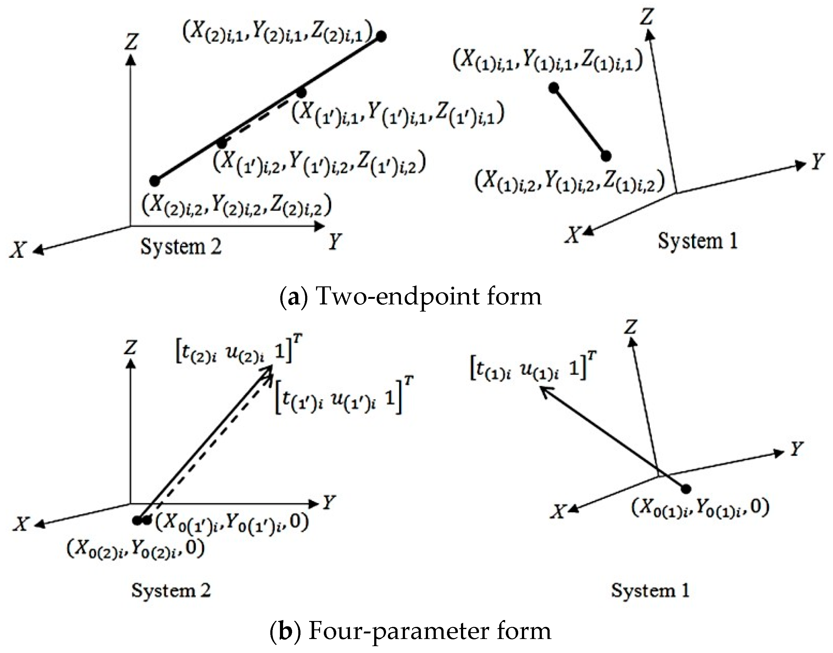
Figure 3.
Normal vector and polar forms of the plane-based transformation.
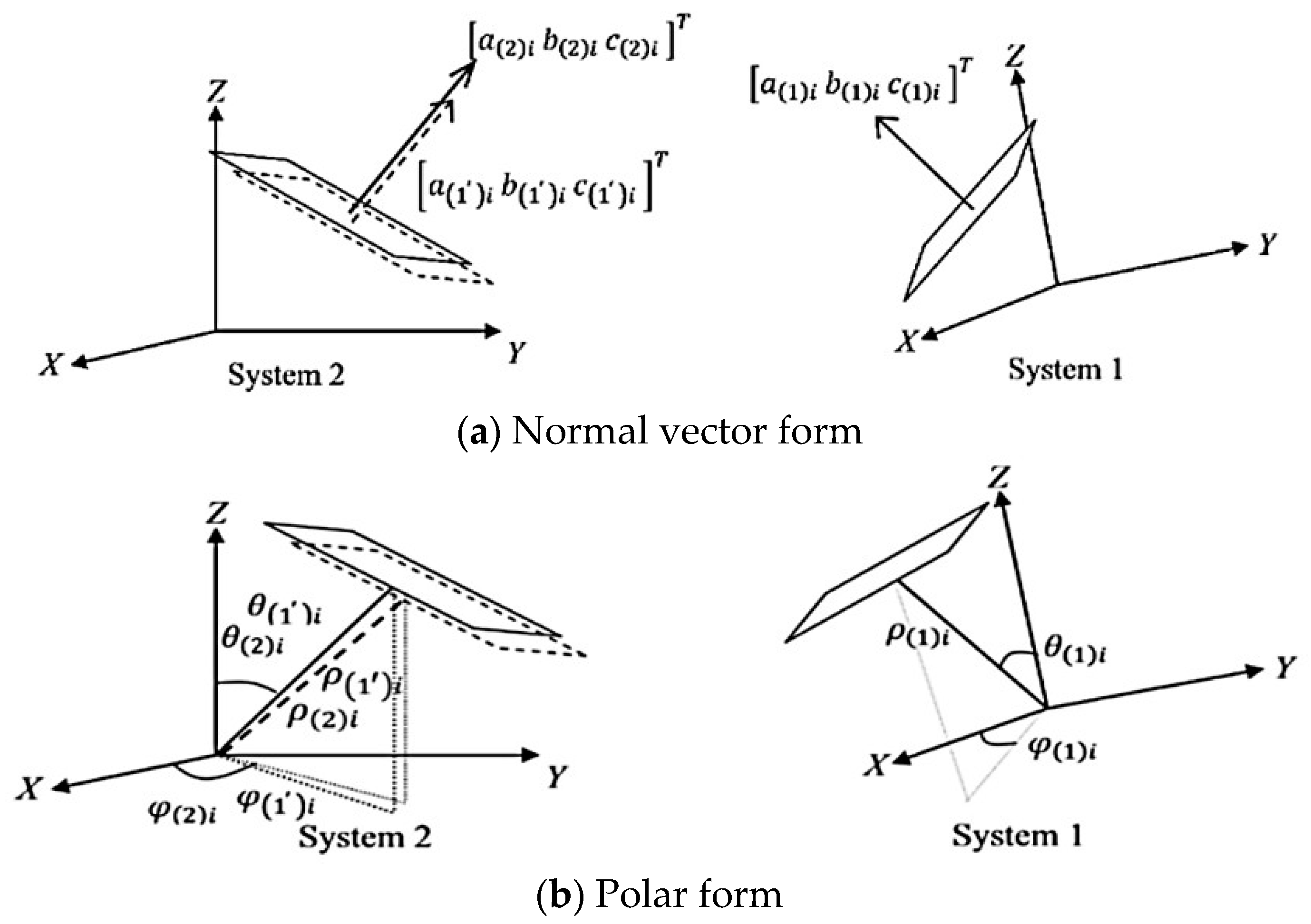
Figure 4.
Illustrations of experimental configurations.

Figure 5.
Quality assessment.

Figure 6.
Quality assessment (r indicates the redundancy).

Figure 7.
Illustrations of feature combinations.

Figure 8.
Assessment of the transformation quality of feature combinations.

Figure 9.
The structure for feature acquisition.

Figure 10.
Illustration of the terrestrial scans.
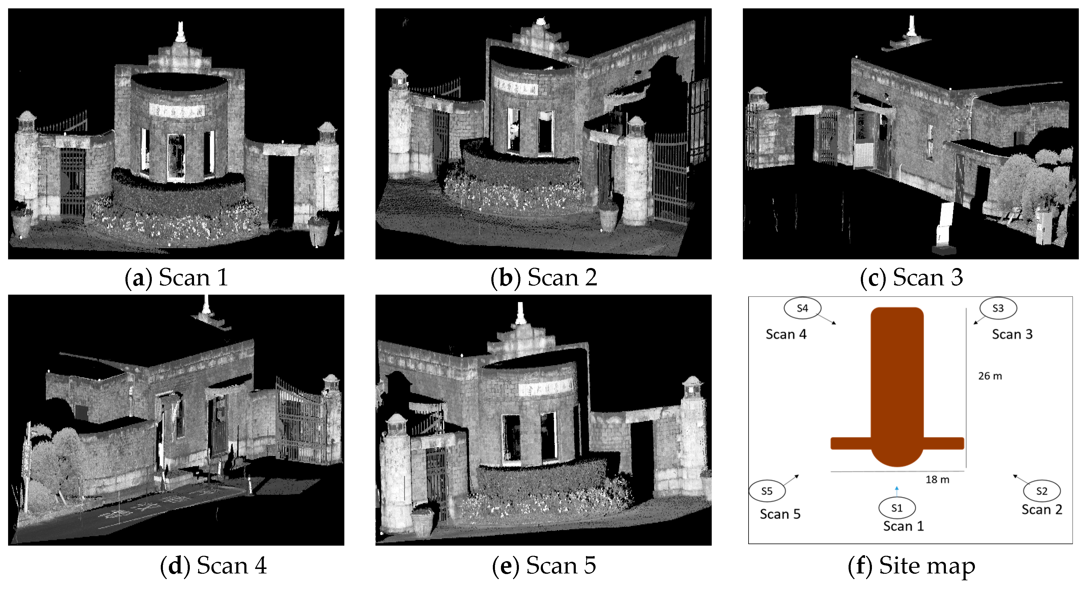
Figure 11.
The feature extraction and matching results.

Figure 12.
The registration results by the proposed method.

Figure 13.
Terrestrial and airborne LiDAR point clouds.
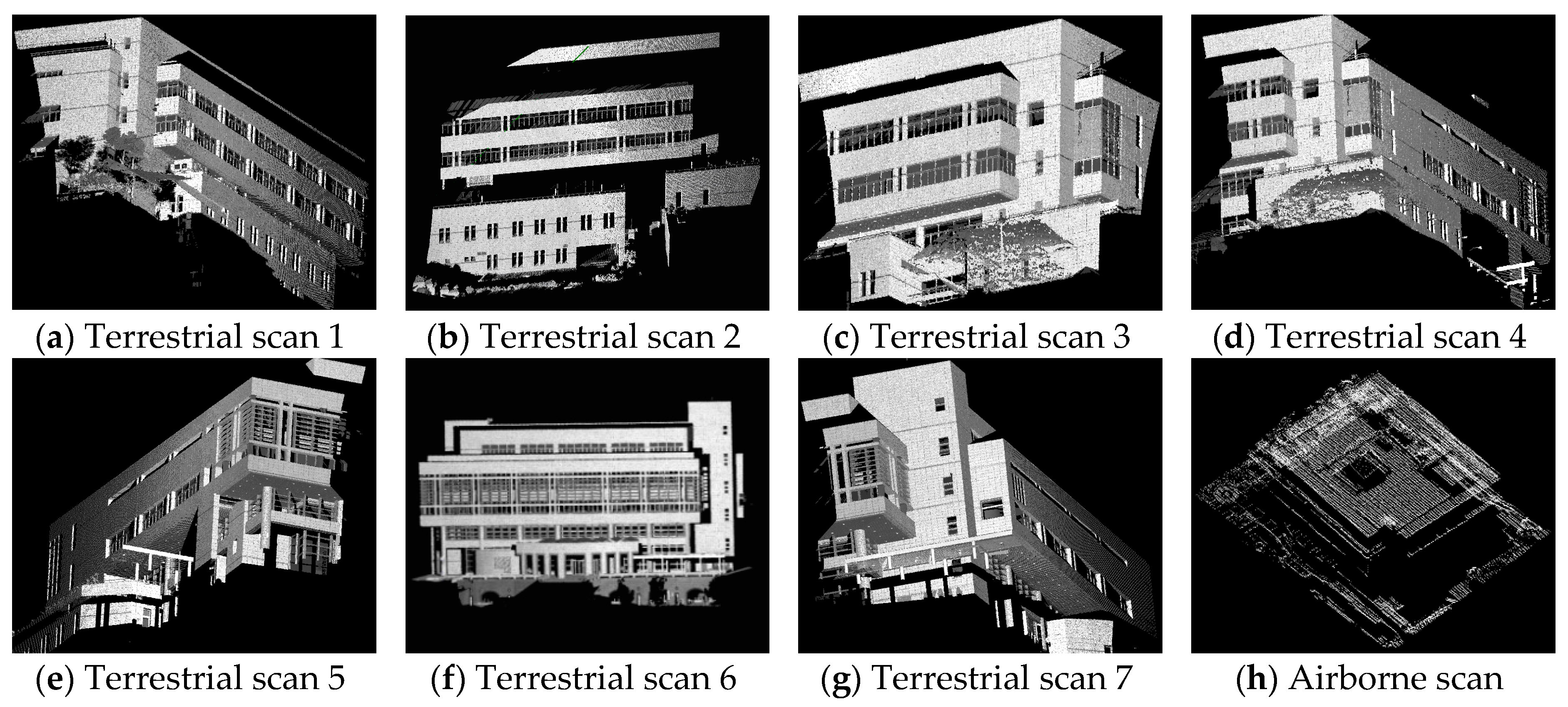
Figure 14.
The feature extraction results.

Figure 15.
The feature matching results.

Figure 16.
The discrepancies in each scan pair.

Figure 17.
The terrestrial registration results reviewing from different directions.

Figure 18.
The feature correspondences and check features.

Figure 19.
The visual inspections on the registered point clouds.

Figure 20.
Mobile and airborne LiDAR data.

Figure 21.
Cross-platform LiDAR registration.

| Penetration Plane | Parameter | Constant |
|---|---|---|
| X–Y | , , , | , |
| Y–Z | , , , | , |
| X–Z | , , , | , |
| Mode | Number of Equations | Redundancy | Number of Features for a Minimum Solution as ns = 2 |
|---|---|---|---|
| Point-based | 3 | ||
| Line-based | 2 | ||
| Plane-based | 4 |
| Scan 1 | Scan 2 | Scan 3 | Scan 4 | Scan 5 | |
|---|---|---|---|---|---|
| Number of points | 529,837 | 624,229 | 1,432,191 | 1,105,417 | 635,438 |
| Avg. scanning distance (m) | 26.0 | 29.7 | 21.9 | 22.6 | 28.2 |
| Density (pts./m2) | 8726 | 1190 | 2475 | 2383 | 1409 |
| Avg. point spacing (cm) | 1.1 | 2.9 | 2.0 | 2.0 | 2.7 |
| Nominal positional accuracy (mm) | 2.6 | 3.0 | 2.2 | 2.3 | 2.8 |
| MSE (cm) | IA-/std. (cm) | /std. (deg.) | /std. (cm) | RMSE_P (cm) | |
|---|---|---|---|---|---|
| ICP | 0.01 | - | 0.48/0.04 | 1.30/0.23 | 1.36 |
| Line-based | - | 0.87/0.13 | 0.32/0.02 | 1.09/0.18 | 1.17 |
| Proposed method | - | 0.75/0.12 | 0.31/0.02 | 1.04/0.15 | 1.03 |
| Scan | Number of Points | Avg. Scanning Distance (m) | Avg. Point Spacing (cm) | Nominal Positional Accuracy (mm) |
|---|---|---|---|---|
| Terrestrial scan 1 | 543,001 | 37.366 | 9.0 | 2.9 |
| Terrestrial scan 2 | 574,007 | 37.716 | 6.7 | 3.0 |
| Terrestrial scan 3 | 565,367 | 37.831 | 5.5 | 3.0 |
| Terrestrial scan 4 | 511,254 | 37.601 | 9.1 | 3.0 |
| Terrestrial scan 5 | 484,352 | 33.779 | 7.3 | 2.7 |
| Terrestrial scan 6 | 1,745,490 | 94.370 | 4.6 | 7.5 |
| Terrestrial scan 7 | 728,603 | 36.145 | 7.7 | 2.9 |
| Airborne scan | 37,678 | 450 | 44.7 | 237 |
| T-1 | T-2 | T-3 | T-4 | T-5 | T-6 | T-7 | A-1 | Total | |
|---|---|---|---|---|---|---|---|---|---|
| Point | 11 | 1 | 9 | 8 | 4 | 0 | 7 | 3 | 43 |
| Line | 33 | 23 | 35 | 29 | 23 | 15 | 22 | 13 | 193 |
| Plane | 7 | 6 | 11 | 10 | 7 | 5 | 9 | 6 | 61 |
| Total | 51 | 30 | 55 | 47 | 34 | 20 | 38 | 22 | 297 |
| Parameters | (rad) | (rad) | (rad) | (m) | (m) | (m) | ||
|---|---|---|---|---|---|---|---|---|
| Scan 1-6 | 1.0151 | −3.4493 | 2.8075 | −1.6508 | −94.612 | 53.321 | −18.798 | 0.855 |
| Scan 2-6 | 1.0098 | −3.2476 | 2.9891 | −1.8388 | −71.119 | 34.458 | −12.529 | |
| Scan 3-6 | 0.9987 | −3.1344 | 9.4287 | −15.905 | 0.10513 | 0.0277 | 0.3087 | |
| Scan 4-6 | 0.9975 | 18.248 | −12.14 | 2.3005 | −68.693 | 126.67 | −53.181 | |
| Scan 5-6 | 1.002 | −3.0229 | −3.559 | −14.151 | −152.29 | 88.494 | −13.467 | |
| Scan 7-6 | 1.0012 | 2.8475 | 15.355 | −7.9346 | −93.779 | 53.096 | −17.995 |
| Parameters | (rad) | (rad) | (rad) | (m) | (m) | (m) | ||
|---|---|---|---|---|---|---|---|---|
| Scan 1-6 | 1.0 | −3.4493 | 2.8075 | −1.6508 | −94.614 | 53.323 | −18.798 | 0.894 |
| Scan 2-6 | 1.0 | −3.2476 | 2.9891 | −1.8388 | −71.118 | 34.456 | −12.530 | |
| Scan 3-6 | 1.0 | −3.1344 | 9.4287 | −15.905 | 0.105 | 0.028 | 0.310 | |
| Scan 4-6 | 1.0 | 18.248 | −12.14 | 2.3005 | −68.692 | 126.67 | −53.180 | |
| Scan 5-6 | 1.0 | −3.0229 | −3.559 | −14.151 | −152.290 | 88.495 | −13.466 | |
| Scan 7-6 | 1.0 | 2.8475 | 15.355 | −7.9346 | −93.779 | 53.097 | −17.995 |
| MSE (cm) | IA-/std. (cm) | /std. (deg.) | /std. (cm) | |
|---|---|---|---|---|
| ICP | 3.31 | - | 9.30/1.31 | 6.82/2.42 |
| Line-based | - | 1.97/0.23 | 0.64/0.40 | 2.04/0.27 |
| Proposed method | - | 1.35/0.11 | 0.42/0.31 | 1.61/0.21 |
| Proposed method () | - | 1.61/0.47 | 0.44/0.39 | 1.73/0.64 |
| IA-/std. (cm) | /std. (deg.) | /std. (cm) | |
|---|---|---|---|
| ICP | - | - | - |
| Line-based | 11.13/1.13 | 2.03/0.07 | 12.48/1.32 |
| Proposed method (unweighted) | 12.73/3.41 | 2.06/0.04 | 13.62/1.79 |
| Proposed method (weighted) | 11.12/1.11 | 2.02/0.03 | 11.23/1.24 |
| Scan | Number of Points | Avg. scanning Distance (m) | Avg. Point Spacing (cm) | Nominal Positional Accuracy (cm) |
|---|---|---|---|---|
| Mobile scan | 2,911,811 | 47.7 | 3 | 24 |
| Airborne scan | 766,488 | 385 | 40 | 19.8 |
| IA-/std. (cm) | /std. (deg.) | /std. (cm) | |
|---|---|---|---|
| Proposed method | 6.33/1.01 | 0.017/0.002 | 8.72/1.18 |
© 2017 by the authors. Licensee MDPI, Basel, Switzerland. This article is an open access article distributed under the terms and conditions of the Creative Commons Attribution (CC BY) license ( http://creativecommons.org/licenses/by/4.0/).
Share and Cite
MDPI and ACS Style
Chuang, T.-Y.; Jaw, J.-J. Multi-Feature Registration of Point Clouds. Remote Sens. 2017, 9, 281. https://doi.org/10.3390/rs9030281
AMA Style
Chuang T-Y, Jaw J-J. Multi-Feature Registration of Point Clouds. Remote Sensing. 2017; 9(3):281. https://doi.org/10.3390/rs9030281
Chicago/Turabian StyleChuang, Tzu-Yi, and Jen-Jer Jaw. 2017. "Multi-Feature Registration of Point Clouds" Remote Sensing 9, no. 3: 281. https://doi.org/10.3390/rs9030281
Note that from the first issue of 2016, this journal uses article numbers instead of page numbers. See further details here.