Article

Supervised Sub-Pixel Mapping for Change Detection from Remotely Sensed Images with Different Resolutions

1
Institute of Geophysics and Geomatics, China University of Geosciences, Wuhan 430074, China
2
Department of Electrical and Computer Engineering, Mississippi State University, Starkville, MS 39759, USA
*
Author to whom correspondence should be addressed.
Remote Sens. 2017, 9(3), 284; https://doi.org/10.3390/rs9030284
Submission received: 31 January 2017 / Revised: 9 March 2017 / Accepted: 15 March 2017 / Published: 17 March 2017
(This article belongs to the Special Issue Remote Sensing Big Data: Theory, Methods and Applications)

Abstract

:
Due to the relatively low temporal resolutions of high spatial resolution (HR) remotely sensed images, land-cover change detection (LCCD) may have to use multi-temporal images with different resolutions. The low spatial resolution (LR) images often have high temporal repetition rates, but they contain a large number of mixed pixels, which may seriously limit their capability in change detection. Soft classification (SC) can produce the proportional fractions of land-covers, on which sub-pixel mapping (SPM) can construct fine resolution land-cover maps to reduce the low-spatial-resolution-problem to some extent. Thus, in this paper, sub-pixel land-cover change detection with the use of different resolution images (SLCCD_DR) is addressed based on SC and SPM. Previously, endmember combinations within pixels are ignored in the LR image, which may result in flawed fractional differences. Meanwhile, the information of a known HR land-cover map is insignificantly treated in the SPM models, which leads to a reluctant SLCCD_DR result. In order to overcome these issues, a novel approach based on a back propagation neural network (BPNN) with different resolution images (BPNN_DR) is proposed in this paper. Firstly, endmember variability per pixel is considered during the SC process to ensure the high accuracy of the derived proportional fractional difference image. After that, the BPNN-based SPM model is constructed by a complete supervised framework. It takes full advantage of the prior known HR image, whether it predates or postdates the LR image, to train the BPNN, so that a sub-pixel change detection map is generated effectively. The proposed BPNN_DR is compared with four state-of-the-art methods at different scale factors. The experimental results using both synthetic data and real images demonstrated that it can outperform with a more detailed change detection map being produced.

Graphical Abstract

1. Introduction

With the development of remote sensors for Earth observations, high resolution (HR) land-cover change detection (LCCD) has become very common. Sensors, such as WorldView and GeoEye, can capture images with high temporal and spatial resolution, but the high cost limits their extensive applications [1]. Moreover, the narrow swath of these sensors cannot meet the demand of LCCD for large areas. Therefore, many low resolution (LR) images are still used for land-cover monitoring. Many change detection (CD) techniques have been developed, such as post-classification comparison [2], change vector analysis [3], and ecosystem monitoring models [4]. These commonly used methods are considered “full-pixel level” approaches, because the determination of change or no-change takes place at the pixel level. For example, post-classification change detection assigns a pixel to a single class, and the change information at the pixel level is obtained after comparing each pixel pair at different times. It is worth noting that a remotely sensed image usually contains a large number of mixed pixels due to rough spatial resolution. Therefore, a loss of information and low CD accuracy are inevitable during such a “full-pixel level” process, since a mixed pixel is composed of several classes but mistakenly considered as a single class [5].
Soft classification (SC) techniques have been utilized to deal with this problem by estimating proportions of each type of land-cover within a pixel. It can provide information at the sub-pixel level and therefore be useful for a more detailed analysis of CD [6,7,8]. SC methods often rely on post-SC comparison or a posterior probability comparison. Correspondingly, change information is exploited from the “full-pixel level” to the “sub-pixel level”. However, only the changed proportions are provided, and there is no indication about the spatial distribution of changed land-cover classes within a pixel. Therefore, sub-pixel mapping (SPM) techniques have been proposed to estimate spatial distribution of land-cover classes within a coarse pixel [9,10,11,12], where each sub-pixel can address a given reasonable situation within the pixel and the resolution of the resulting classification map is enhanced. Based on this concept, sub-pixel land-cover change detection (SLCCD) is developed by integrating SC and SPM. An intuitive strategy is to obtain fractional difference images using the SC, and construct a HR land-cover change map using the SPM.
It is noted that the fine resolution image information at another time can be utilized to improve the accuracy of SLCCD. A common practice is that a historical HR image or map is the baseline, while recent images are LR images [13]. SLCCD with multi-temporal images at different resolutions (SLCCD_DR) can combine an HR land-cover map and an LR image to detect change/no-change and from-to information at high resolution. Recently, several works have focused on this issue. For instance, the pixel swapping algorithm (PSA) model was first proposed to analyze the sub-pixel configuration estimated from two temporal images with different resolutions [14]; a cellular automata (CA) model was modified to simulate the changed sub-pixel location with two different spatial resolution images [15]; the Hopfield neural network (HNN) model was analyzed to show an excellent capability to investigate sub-pixel changes [16,17]; and five fast SPM algorithms (i.e., bilinear interpolation, bicubic interpolation, sub-pixel/pixel spatial attraction model, Kriging, and radial basis function interpolation methods) were compared for sub-pixel CD [18]. Meanwhile, the minimum energy function was designed by utilizing restrictions on SC and SPM to reduce the effect of the cumulative error [19,20]. The SLCCD_DR model using sub-pixel scale information from the prior HR image or map is demonstrated to yield better performance compared to the traditional SLCCD model.
Although these SLCCD_DR techniques are successful to certain degrees, they include some limitations. (1) None of them take full advantage of the prior HR image in the SLCCD_DR model. These methods are all designed in an unsupervised framework, directly relying on spatial dependence or spatial correlation between pixels in the LR image. The known HR image is utilized for increasing the SLCCD_DR accuracy, but they do not take an HR image as an additional information source. (2) They ignore the change of endmember combinations when decomposing a candidate pixel. The form of endmember combinations in the LR image is mistakenly assumed to be fixed. When the scale factor of the LR image magnification is large, it may become challenging to secure a high quality land-cover change map based on SPM. (3) They generally assume an HR image is taken earlier than the LR image. With the rapid development of Earth observation sensors, it is common that the HR image postdates the LR images.
In this paper, we propose a novel SLCCD_DR approach based on a back propagation neural network (BPNN) to overcome these limitations. The proposed method is based on the assumption that the LR image and HR map contain the same number and types of land-cover classes. The LR land-cover map can either predate or postdate the HR image. First, the selection of the endmember set per pixel is introduced into the SC method to estimate the proportions of the LR image. After that, the fractional difference images are incorporated with several SLCCD_DR rules based on the supervised BPNN model for SPM.
The remainder of this paper is organized as follows. In Section 2, the fractional difference images are described, including the endmember combination of the LR image and the computation of differences in the proportions. In Section 3, the SPM method for SLCCD_DR based on a BPNN is proposed. In Section 4, a summary of the entire framework is provided. In Section 5, two experiments with synthetic and real image data are described. The conclusions are drawn in Section 6.

2. The Fractional Difference Image

2.1. The Endmember Combination of the LR Image

The reflectance spectrum of a mixed pixel in the LR image is regarded as a combination of the component spectra in the mixture. Here, these distinct components of certain materials are called endmembers. To find the real endmember combination, the number of endmembers and their signatures in each pixel should be estimated before SC is performed. Over the past few years, several endmember selection algorithms have been proposed for this purpose [21,22], where the endmember average root mean squared error (RMSE) was used as the selection criterion; during the process, there were a large number of candidate endmembers with each endmember class having several optional signatures. Our method differs significantly in that it can quickly extract optimal endmember compositions from a pre-defined global endmember set; each endmember corresponds to a single class spectral signature, and model fitting is assessed by direct comparison in terms of the spectral similarity of endmember classes in the pixels.
More specifically, the process is described as follows. Firstly, the N-finder algorithm (N-FINDR) algorithm is used to extract global endmembers in the scene [23]. Let the extracted endmembers construct an initial endmember reference set E, which is regarded as a reference set. The number of extracted endmember materials can also be reduced if prior information about the endmember classes is known. A cross-correlogram spectral matching (CCSM) technique is adopted as a spectral similarity metric to compare a known reference material and an unknown material underlying a pixel, with a cross correlation coefficient C being defined as [24]:
C = N r r r t r r r t [ N r r 2 ( r r ) 2 ] [ N r t 2 ( r t ) 2 ]
where r r and r t are the reference and test spectral signatures in the image, respectively, and N is the number of bands. The larger the cross correlation coefficient C is, the more similar the two signatures are. The spectral matching process can be regarded as a projection on a particular direction. Each candidate pixel is projected onto all available normal endmember vectors, and the contributions of all the endmembers from CCSM are lined up based on Equation (1). The most efficient projection, corresponding to the one with the highest value, indicates the first selected endmember (SE). The influencing factors of the chosen endmember are subtracted from the testing pixel spectrum, which means to normalize the spectral vector with the maximum projection. After that, the residual pixel spectral signature is used to select the second endmember by repeating the projection onto all remaining endmember normal vectors, and so on. The remaining pixel spectral signature is:
r t = r t C max e max
where r t is the residual pixel spectral signature, C max is the maximum cross correlation value, and e max is the largest endmember of the dataset. Previously selected spectral components are removed and are no longer considered in the latter selection. These steps are repeated until the remaining spectral signature is minor or even negative. In the end, the number of endmembers and endmember signatures can be estimated.

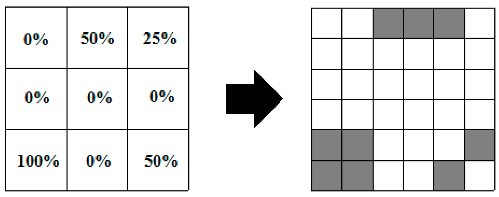
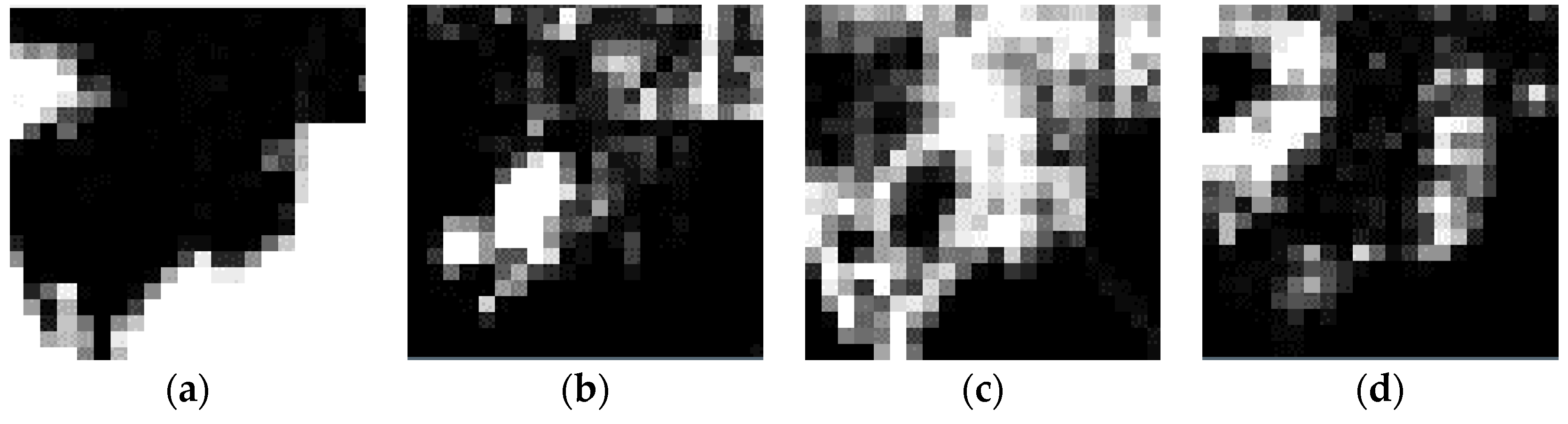
2.2. Computation of the Differences in the Proportions

The linear mixture model (LMM) has been applied to estimate the component proportions within mixed pixels due to simplicity and effectiveness [25]. For the pixel-specific LMM, a mixed pixel r is expressed as
r = + n
where M is the variable endmember matrix specific to r, α is an abundance column vector which is composed of each endmember’s abundance, and n is the noise term. An ordinary least squares method can be used to estimate α. Furthermore, to keep the physical meaning of the LMM, two constraints on abundances, i.e., non-negative and sum-to-one, are both imposed [26]. Consequently, the LMM model is constructed according to pixel-specific endmembers. That is, the SE subset is introduced to the constrained LMM to decompose the candidate pixels, called LMM_SE. If an endmember class is not included in a pixel, the corresponding proportion is considered equal to 0. The final abundances of all endmembers are fused. In this way, the proportions of each land-cover in the LR image are acquired.
Meanwhile, the HR land-cover classification map is downscaled in order to estimate the proportions of land-cover classes in each pixel. The comparison is performed on each pixel pair in LR and HR images to generate the initial fractional difference images of each land-cover. Let α k _ f and α k _ l be the former and latter proportions of the k-th class, respectively. The fractional difference image value of the k-th class D k is:
D k = α k _ l α k _ f
An appropriate threshold is set based on the histogram of the difference image to avoid false change and noise. Since the intensity change values often follow the Gaussian mixture model, the expectation maximization (EM) algorithm and Bayes discriminant criterion are used to estimate the threshold of each land-cover change [27,28]. If the absolute value of Dk is larger than the threshold, it is considered significant, indicating a certain change. Otherwise, it is regarded as zero.

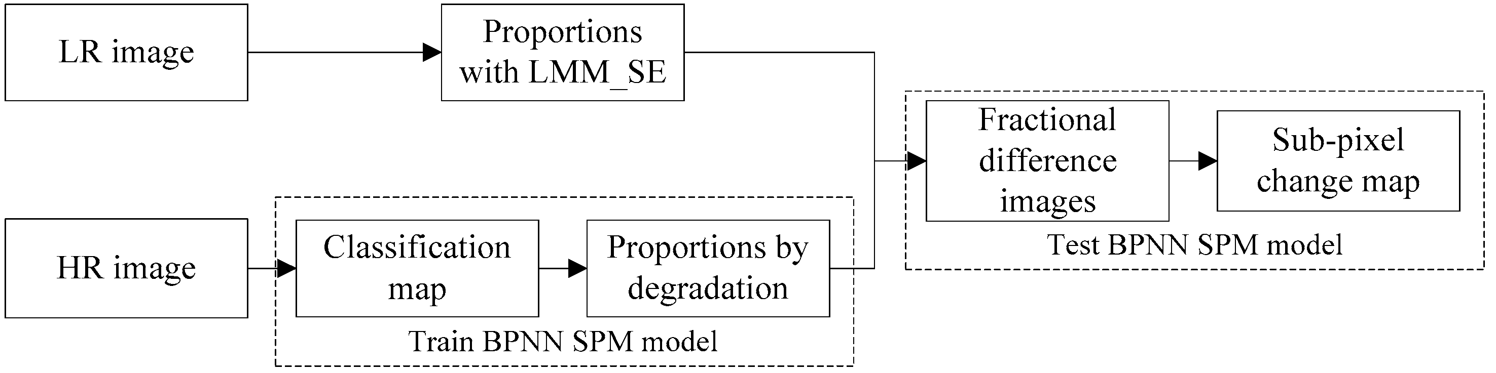
3. Sub-Pixel Mapping for SLCCD_DR Based on BPNN

3.1. Sub-Pixel Mapping

As stated by Atkinson in 1997, SPM can be seen as a technique where mixed pixels are divided into smaller ones, called sub-pixels, and different land-covers are spatially allocated in the sub-pixel level in such a way that spatial dependence is maximized [29]. The resulting map is regarded as a higher resolution representation of a parent pixel. The spatial dependence is the key issue of SPM, i.e., the tendency of spatially proximate observations of a given property to be more alike than more distant observations [30].
Assume there are S 2 sub-pixels per pixel, where S is the scale factor in the row or column direction. A simple representation of the SPM problem using a 3 × 3 set of pixels is given in Figure 1, where the associated proportions of a land-cover class are produced by SC and the scale factor is S = 2 . A single pixel is thus divided into four sub-pixels, each corresponding to 1/4 of the coverage of the pixel. The value for a sub-pixel ( x i j ) is determined according to the following rule: if sub-pixel j is assigned to land-cover class i, the value of x is equal to 1, otherwise it is 0. Summing x i j for all S 2 sub-pixels yields the spatial dependence for that specific sub-pixel configuration inside the pixel, i.e.,
η i = j = 1 S 2 x i j
Each arrangement yields a fraction value η i , with the aim to finding the optimal super-resolution configuration whilst retaining the original fraction values.

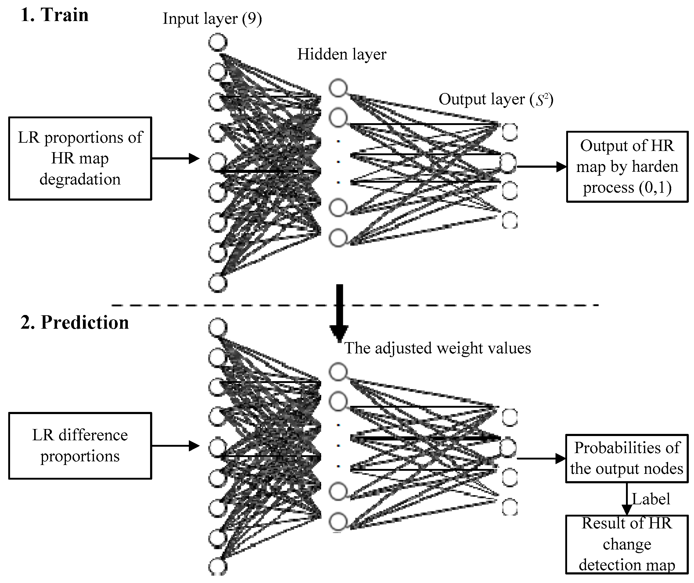
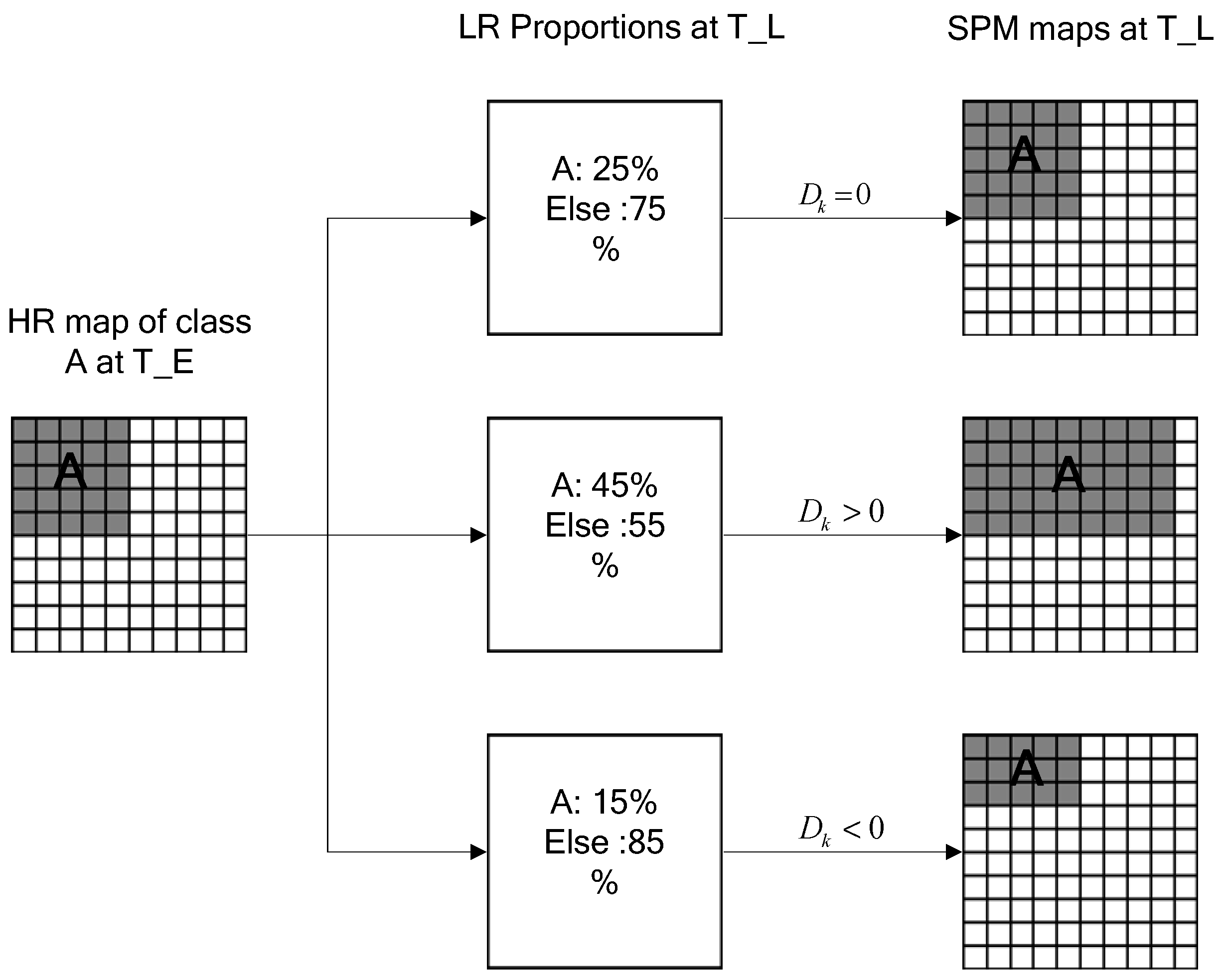
3.2. BPNN-Based Sub-Pixel Mapping Model

In the past few years, BPNN has been demonstrated to be a powerful tool for prediction of sub-pixel configuration [31,32]. According to the spatial dependence principle, BPNN is applied to construct a local SPM model that describes the relationship between fractions in a local window and the spatial distribution of sub-pixels assigned to the target in the central pixel. Therefore, the sub-pixel value is determined by the corresponding central pixel and its neighboring pixels. The larger the proximate neighboring pixel value is, the more likely the sub-pixel assigned to the target class is, which makes the spatial dependence reach a maximum. For convenience, it is explained as a simple expression (6). Let the scale factor S be 2. Under this condition, every neuron representing a coarse pixel is affected by the eight neighbors and their influence is different. The nine neurons in a fractional image are taken as the input of the network, according to the centered neuron:
[ x i 1 , j 1 x i 1 , j x i 1 , j + 1 x i , j 1 x i , j x i , j + 1 x i + 1 , j 1 x i + 1 , j x i + 1 , j + 1 ] [ o 1 o 2 o 3 o 4 ]
where i and j are the column and row of the image, x is the proportions of the LR image, and o is the label value (0 or 1). There are four sub-pixels in the model, and the k-th output node is defined as o k , k = 1–4. If it belongs to the target class, o k = 1; otherwise, o k = 0. Obviously the number of the input nodes in the network is fixed, but the number of the output nodes is determined by the factor size. The mathematical model of the output layer nodes o k is described as:
o k = f ( n e t k )
n e t k = j = 1 p w j k y j γ k
f ( x ) = 1 1 + e x
where f ( . ) is a nonlinear activation function, which is commonly a sigmoid function, x is the input vector to the network, y j is the j-th output from the hidden layer, o k is the k-th output from the output layer, w j k is the connection weight from the j-th hidden node to the k-th output node, and γ k is the threshold value of the k-th output node. To find the most reasonable pattern of SPM, a suitable metric, e.g., the sum of square error (SSE) E, can be defined as:
E = h T O 2 / 2
where T = [ t 1 , t 2 , t 3 , t 4 ] is the target output pattern vector, O = [ o 1 , o 2 , o 3 , o 4 ] is the output pattern vector of the network, and h ranges over all vectors in the training set. Thus, finding the optimal SPM is equivalent to minimizing the E. This spatial distribution rule can be obtained through network training and be finally stored in connection weights.

3.3. The Architecture of BPNN for SLCCD_DR

The BPNN model is composed of three layers: input, hidden, and output layers. Two important parameters, i.e., the number of hidden layers and the number of nodes in each hidden layer, should be decided. Previous studies show that one hidden layer is generally sufficient to solve complex problems if enough nodes are used [33]. Therefore, this paper is only limited to one hidden-layer BPNN and the number of hidden nodes is determined empirically.
In order to obtain the HR change detection map, the LR difference proportions of two different images are input into the model for prediction. However, in our algorithm, the finer scaled version of the change map is not available in real situations. Fortunately, the network can be trained on other data than the source imagery since BPNN can learn relations from offline examples [34]. This does not imply that training of the network is not affected by the image used. The more similar the training and testing images are, the higher the accuracy will be [35]. It is assumed that spatial dependence does not differ between the multi-temporal images and the difference proportion images. Therefore, the HR map and the corresponding degraded proportions are regarded as output and input, respectively, to train the network. In the training process, the LR proportions (0–1) are propagated as input values through the network in the feed-forward phase. The output of the model is the HR map (0 or 1) by the hardening process. The error of the calculated output, according to the desired output, is back-propagated from the output layer to the hidden layer to adjust the weights in the opposite direction of signal flow with respect to each individual weight. By repeatedly applying this procedure for each pattern in the training set, the learning process can converge.
In the prediction process, the LR difference proportions of two different images are input to the BPNN to obtain the output value. Although there is a significant difference between the fractional difference image and the HR map trained, the assumption of spatial dependence still holds. This implies that training of the BPNN is not affected by the image used. The input pattern is normalized to (0–1) to ensure that similar training samples can be obtained. The output nodes are exported in the form of the probability in the HR map, but each sub-pixel of an output pattern is not integral. To resolve this issue, the land-covers of these sub-pixels are labeled according to the input proportion. The architecture of a three-layer BPNN for SLCCD_DR is shown in Figure 2.

3.4. The SLCCD_DR Hypothesis

Several simple and efficient change detection rules are introduced to incorporate the HR sub-pixel spatial distribution in SPM [16]. Through analyzing the proportion difference D k in Equation (4) at two different times, each sub-pixel is guided to label changed or unchanged for the k-th class. Let T_E and T_L be the early time and the later time in the change detection model, respectively. There are three different conditions. (1) If D k = 0 , no change pixel exists, and all sub-pixel locations of the class in T_E are the corresponding sub-pixel locations of the class at T_L; (2) If D k > 0 , part of the sub-pixel locations at T_L of the class are still the corresponding sub-pixel locations at T_E, and the remaining increased sub-pixels are transformed from other sub-pixels; (3) If D k < 0 , some sub-pixels at T_E have transformed to other classes, and all of the sub-pixel locations at T_L are within the area of the class at T_E. Thus, a specific SPM algorithm should be defined based on the fractional difference image in the first and third categories.
An illustration is shown in Figure 3. The left image is the HR map at time T_E, which shows a mixed pixel divided by 10 × 10 sub-pixels. Class A is shown in a gray grid, and the else classes are in a white grid. Based on the number of sub-pixels within a pixel, the area percentage of class A is determined. The percentage of class A is 25% and the else class is 75%, respectively. The middle images are the LR images at time T_L, which show the area percentages of class A and the else classes for three cases. In the first case, D k = 0 , no changes occur for class A; in the second case, D k = 20 / 100 , the increased 20 sub-pixels are transformed from other sub-pixels and 25 sub-pixel locations remained in the original position at time T_L; in the third case, D k = 10 / 100 , 10 sub-pixels have transformed to other classes, while no pixels of the other classes should be transformed into the original class. According to the above three cases, there are different SPM results at time T_L on the right.

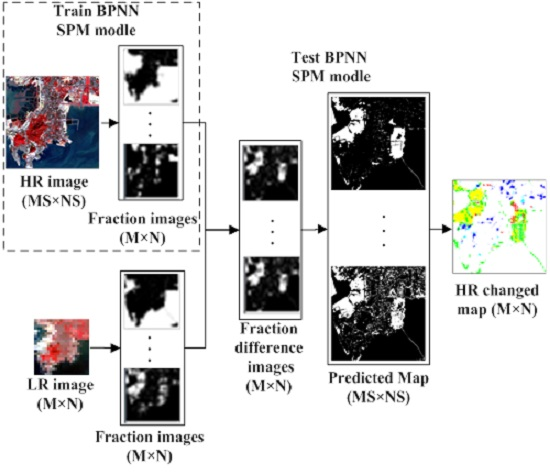
4. The Flowchart of the Proposed Algorithm

The complete framework of the proposed BPNN algorithm with different resolution images, called BPNN_DR, is summarized in Figure 4. Assume there are two remotely sensed images with different spatial resolutions (LR and HR) covering the same area. The land-cover proportions of each pixel in the LR image are estimated using the LMM_SC. Meanwhile, the HR classification map is degraded to produce the map with the same resolution of the LR image but with known land-cover proportions per pixel. Then the fractional difference image is generated based on these two types of proportions. The BPNN-based SPM is performed according to the proportion differences. In the training process, the degraded proportions and the HR classification map are the input and output data of the BPNN, respectively; in the testing process, the LR proportion differences are the input data, and the output is the HR land-cover change information.

5. Experiments and Analysis

In our experiment, four state-of-the-art methods are used to compare with the BPNN_DR, including the bilinear interpolation-based model (BI) [36], PSA model [14], and HNN model [17]. In addition, the LR image can be super-mapped using BPNN-based SPM. After that, the sub-pixel change detection map is produced by directly comparing the SPM result with the known HR map. For convenience, it is called the BPNN_SPM model. These methods all borrow information from the HR image to improve the accuracy of the SLCCD.

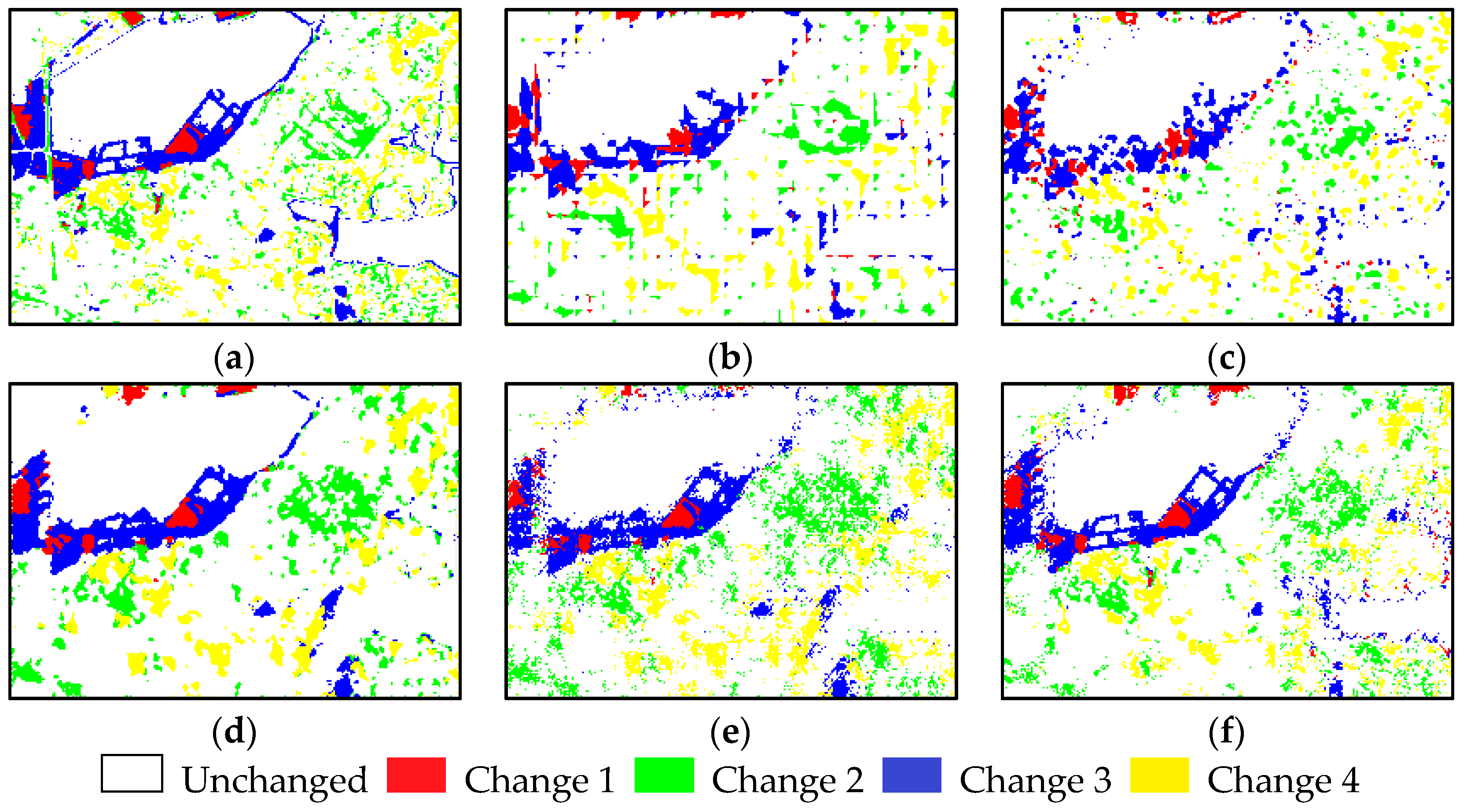
5.1. Synthetic Data Test

The data set consisted of two Landsat Thematic Mapper (TM) images at 30-m spatial resolution, covering the urban area of Wuhan, Hubei, China. A mixed sub-scene (280 columns, 200 lines) with 6 bands was extracted from the original image acquired in 1986 and 2000, respectively (Figure 5a,b). They are classified into three major classes, water (Class 1), vegetation (Class 2), and urban areas (Class 3), using a support vector machine (SVM). The training data are chosen from the images without change. The reference land-cover change map with fine spatial resolution can be extracted by comparing these two classification maps. In this experiment, the HR image postdates the LR one, and is simulated to test the performance of the algorithms. That is, the degraded LR image in 1986 (Figure 5c) and the HR image in 2000 (Figure 5b) are used. As shown in Figure 5c, the LR image is created by degrading Figure 5a with a spatial averaging filter, and the degrading scale factor S = 8.

5.1.1. Effects of the LMM_SE

In this section, we evaluate the effects of the LMM_SE. First, the reference endmember set is constructed by the N-FINDR algorithm. To reduce the computational complexity of the algorithm, three global endmembers corresponding to Class 1, Class 2, and Class 3 are manually extracted to be the initial endmember reference set. Since the studied region in the experiment is small, the total number and types of endmembers remain the same during the time period. Therefore, the number of endmembers of each pixel yields three possible conditions (from 1 to 3), and different endmember combinations are generated by Equations (1) and (2). Next, the LMM_SE method is performed on the LR image. The pixel-level proportion differences of three land-cover classes are obtained by Equation (3). The RMSE is used to measure the similarity between the estimates and the reference values [37], defined as:
R M S E = j = 1 N ( s j t j ) 2 / N
where sj and tj are the resulting and reference proportion differences of a pixel, respectively. Table 1 presents the RMSE of three land-cover classes’ proportion differences. The traditional LMM, when applied to all pixels, produce a normal proportion for all endmember components considered. Using the LMM_SE, we generate one-, two-, and three-endmember models for each pixel. It is obvious that the errors of the LMM_SE model are lower than that of the LMM.
Visual assessment leads to the same conclusion. For illustration purposes, the largest change of land-covers, i.e., the change of water (either increase or decrease), is shown in Figure 6. The reference image in Figure 6a shows the real proportion difference of water, where bright values represent a high proportion difference and vice versa. The obtained difference image based on LMM and LMM_SE are in Figure 6b,c, respectively. Too many unchanged pixels are wrongly detected as changed pixels in Figure 6b. In contrast, the LMM_SE method can provide a better proportion difference of water as shown in Figure 6c, which is very similar to the reference in Figure 6a.

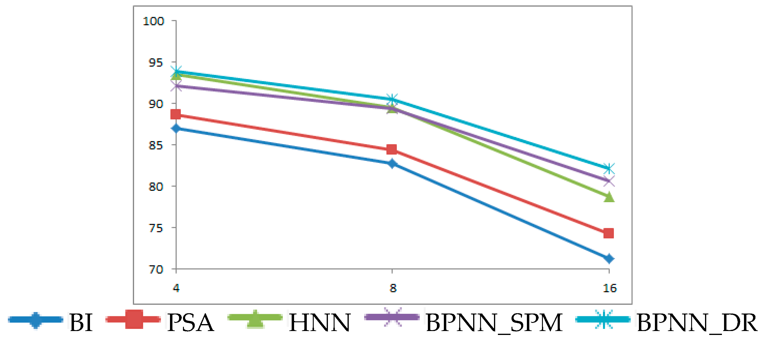
5.1.2. Comparison of the Different SLCCD_DR Methods

After the fractional difference images are produced, whether the difference is significant or not is determined by the EM-estimated threshold (which is 0.13). Four traditional SLCCD_DR methods, i.e., BI, PSA, HNN, and BPNN_SPM, are implemented to compare with the proposed BPNN_DR. For HNN, the weighting constants in the network energy function are set to 1, the steepness of the tanh function is 10, and the number of iterations is set to 1000. For BPNN, the number of neurons in the hidden layer is set as 15, and 200 training samples are randomly selected. In the proposed BPNN_DR algorithm, the degraded LR proportions and the corresponding HR classified image (1 or 0) are used as the input and output of the BPNN model, respectively. After the trained process is finished, the fractional difference images are input for prediction.
Figure 7 shows the reference and change detection maps from these five methods. It is worth noting that water (Class 1) is not increased in reality. Therefore, there are five different colors, describing the unchanged pixels and the different changed pixels. White means unchanged pixels, and the other different colors mean one class changed to another. Specifically, red means Change 1 (Class 1 changed to Class 2), green means Change 2 (Class 3 changed to Class 2), blue means Change 3 (Class 1 to Class 3), and yellow means Change 4 (Class 2 to Class 3). Figure 7a is the reference of the change map. Based on visual inspection, BI produces the worst result in Figure 7b. It leads to blurry change detection maps with a scale of 8, and the spatial properties of the object shapes have been lost. The performance of PSA is better than BI. However, it has the similar limitation that some assembled pixels may not recognize the shape of the changes in Figure 7c. The result of HNN is better than the two former methods because it has the ability to optimize the sub-pixel problem. The HNN produces clear edges of different changes and well discerns land-covers, but it still misses many real isolated pixels as shown in Figure 7d. Due to the same structure, BPNN_SPM and BPNN_DR generate similar change detection maps. The result of BPNN_SPM can distinguish the different changes but cannot detect the accurate position of land-covers, such as Change 3 in Figure 7e. The result of BPNN_DR fixes this problem and discerns different changes well. It yields less misclassified changed areas and generates a more accurate result in Figure 7f.
Performance is quantified with overall accuracy (OA), Kappa value, omission error, and commission, as shown in Table 2 [38]. Comparing the five methods, BI is the worst one as its OA and Kappa values are 82.8% and 0.78, respectively. PSA is a little better than BI. HNN and BPNN_SPM perform very closely, and both are better than BI and PSA. The proposed BPNN_DR provides the best result, and its OA is 90.5%, a gain of 7.7% over BI. The omission errors in BPNN_DR are lower than those in other algorithms, except for Change 4. Because class 4 is always mixed with the other classes in this area, and it is difficult to discriminate their positions. The largest commission error is in Change 1. Any mismatched changes may lead to a large commission error due to the smallest number of pixels in Change 1. Moreover, the proposed algorithm is implemented several times for fair performance assessment. Under the same setting of parameter thresholds, there are very small variations among these results. It means the proposed model is stable and can be used in the experiment.

5.1.3. Different Scale and Computational Efficiency

To better analyze the performance of the BPNN_DR, three different scale factors of 4, 8, and 16 are chosen for testing. As shown in Figure 8, the proposed BPNN_DR is the best one among the five methods. However, the accuracy decreased as the scale factor increased. For instance, based on the BPNN_DR, OA decreases approximately from 93.9% to 82.1% when the factor increases from 4 to 16. So do the other four conventional methods. This shows the difficulty of a large factor for SLCCD_DR. BI offers the worst result with the largest scale factor. The OA of BI with a scale factor of 16 is only about 71.3%. It means that the result is not accurate enough to detect the changes at the sub-pixel scale, especially under such a large scale factor.
The computing time using a Lenovo laptop with Intel(R) Core(TM) i5-4200 CPU @2.4MHz, 8 Gb RAM, Windows 7 OS, and Visual Studio 2010 IDE is shown in Table 3. When the scale factor is increased, each method costs more time. However, the five algorithms have different computing times for each scale factor. BI is the fastest algorithm, because it is a non-iterative and simple strategy. PSA requires more calculation time than BI, because more iterations for computing the nearest spatial correlation are employed. As for HNN, it can reconstruct itself to generate the land-cover changes map, where the self-training and energy minimization process require more calculation time. BPNN_SPM and BPNN_DR both cost more time than the former methods, because they include two main procedures, i.e., offline training and target image processing. In contrast, BPNN_DR can release more computational memory stress than BPNN_SPM, because the latter has to obtain the two land-cover maps at different times and then detect the sub-pixel scale change.

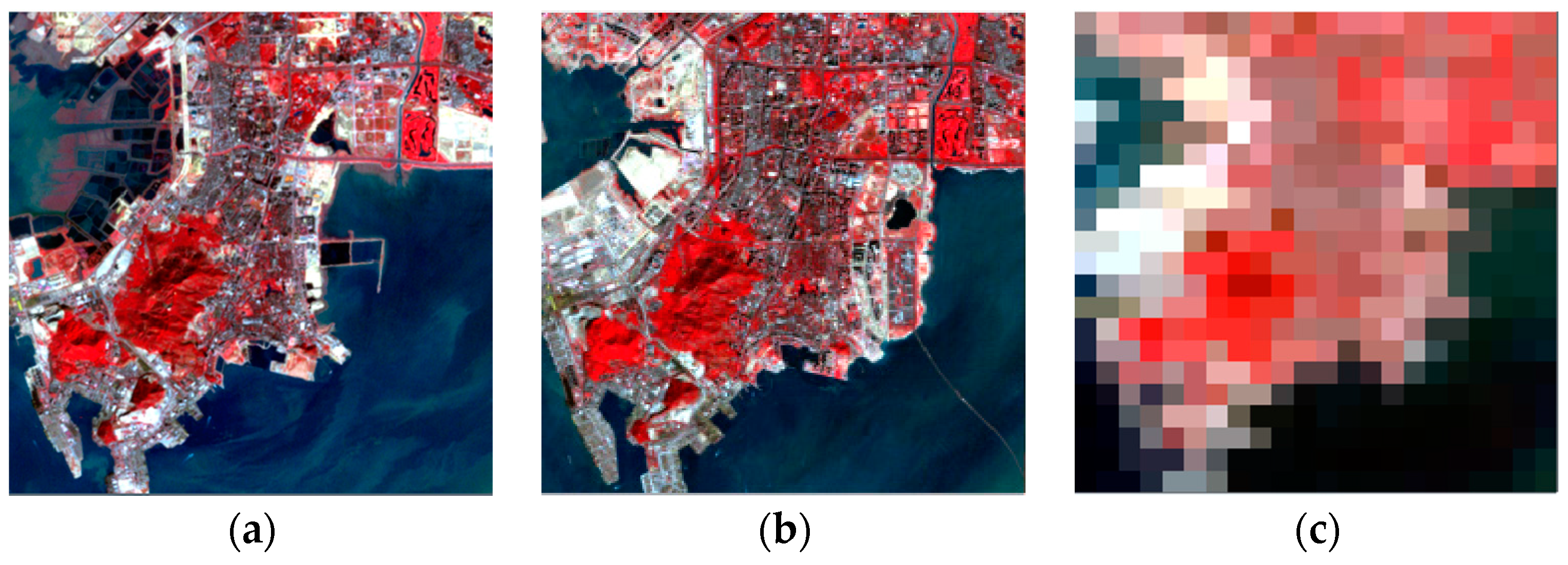
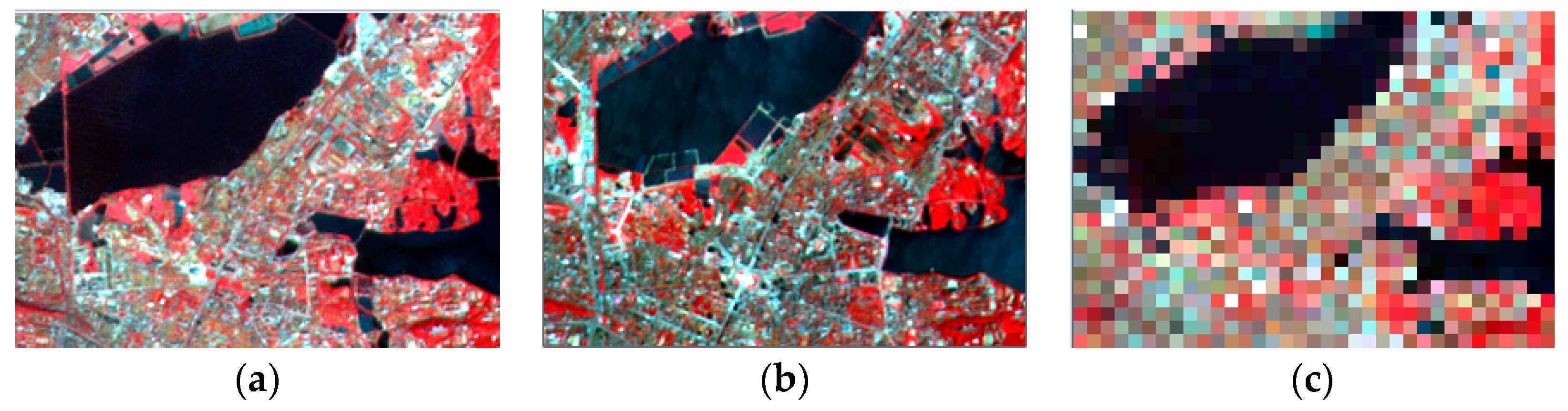
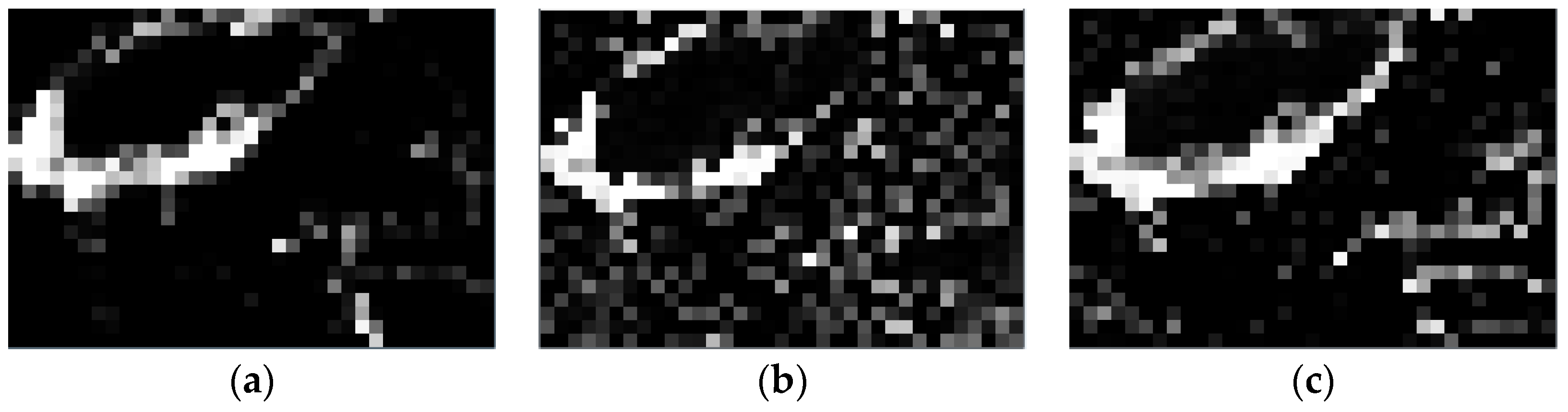
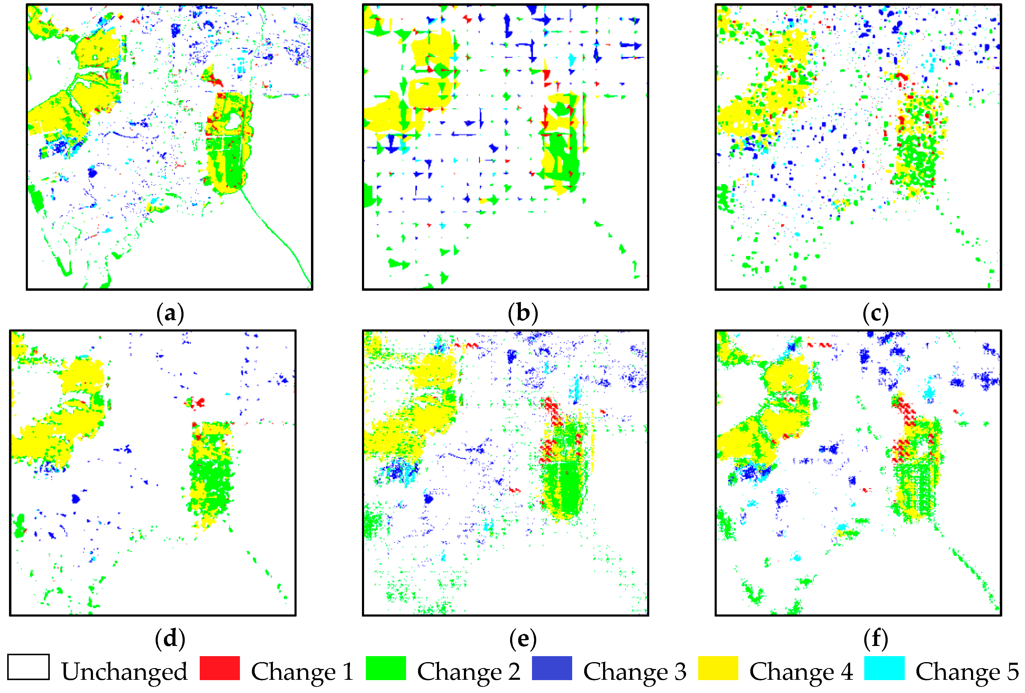
5.2. Real Data Experiment

The real multispectral remotely sensed images, including Landsat TM (30 m) and MODIS (500 m), are also used to evaluate the proposed method after co-registration. The test area is Shenzhen city, Guangdong province, China, which has experienced great land-use/land-cover changes during the past decade. Figure 9a,b show the TM images (408 × 408 pixels) in 2001 and 2009, respectively. The HR reference land-cover change map is produced by comparing these two classification images. Figure 9c shows MODIS images (24 × 24 pixels) in 2001. The color-infrared (CIR) composites of TM and MODIS images are generated with bands 4, 3, 2 and 2, 4, 3, respectively. Unlike the synthetic data test, the HR image (Figure 9a) predated the LR image (Figure 9c) in this experiment. The scale factor is approximately 17. Due to manmade structures (buildings and roads) with high-brightness, the sub-scene includes four major classes: water (Class 1), vegetation (Class 2), urban city (Class 3), and built-up areas (Class 4). In the proposed algorithm, the number of endmembers in each pixel ranges from 1 to 4, yielding four possible conditions. Firstly, the proportion of the entire scene is produced by combining several different unmixing data subsets, which are illustrated in Figure 10a–d. After that, the fractional difference images, which are regarded as the input data for the SPM model, are calculated. The threshold based on the EM algorithm is 0.07. In this experiment, BPNN and HNN use the same initial parameters as in the synthetic experiment. Five hundred training samples of TM image are selected for BPNN. The results are shown in Figure 11, where six different colors display the unchanged and changed pixels. Specifically, white means unchanged pixels, red means Change 1 (Class 1 changed to Class 2), green is Change 2 (Class 1 changed to Class 3), blue is Change 3 (Class 2 changed to Class 3), yellow is Change 4 (Class 1 changed to Class 4), and cyan is Change 5 (Class 2 changed to Class 4).
According to Figure 11, all the methods are effective, but discrepancies are obvious in their performance. The BI result contains plenty of misclassifications of the land-cover changes, as indented holes are introduced into the characters, which is not a desirable feature, always giving a blurry scene. The PSA is better than the BI, but it always aggregates the changed pixels. This is especially apparent when the scale factor is large, such as 17. The HNN provides clear edges of the different land-cover changes, and its result contains less misclassification and makes the border of the classification map smooth. However, some detailed information is lost when compared with the reference image. The BPNN_SPM outperforms the aforementioned methods. Yet there are lots of isolated pixels, which are regarded as a misclassification. Especially, according to Change 2 and Change 3, a set of scattered pixels distributed in the result are incorrectly detected. The performance of BPNN_DR is similar to the BPNN_SPM, but offers a smoother result, illustrating some advantages.
This is also confirmed by the accuracy measures in Table 4. BI still provides the worst result with an OA of 67.3% and a Kappa value of 0.62. PSA is better than BI. The OA of HNN is higher than that of PSA, with a gain of 4.5%. The BPNN_SPM performs better than BI, PSA, and HNN, but it is implemented based on two SPM results at different times and the errors are overlapped. The BPNN_DR offers the best classification accuracy of all the aforementioned algorithms, yielding the highest accuracy of an OA of 80.2% and a Kappa value of 0.76. In general, the omission and commission errors of all methods increase with the increase of the scale factor. With the scale factor S = 17, the largest omission error is 82.6% with BI for Change 1. Meanwhile, the largest commission error is 81.9% with HNN for Change 5. The omission and commission errors of BPNN_DR are lower than that of BI, PSA, HNN, and BPNN_SPM in all cases, except for Change 3.

6. Conclusions

This paper proposes a supervised SLCCD method for multi-temporal images with different resolutions, called BPNN_DR. The key techniques include: SC using linear unmixing and SPM using the BPNN. The SC is used to obtain the land-cover proportion of each pixel in the LR image, where a method of selective endmembers per pixel is applied to ensure accurate estimation. The SPM is achieved by a BPNN, which is trained using the HR image with a known classification map and its degraded LR version with retrieved land-cover proportions. With the trained BPNN, the difference proportions from the estimated SC result and the degraded HR result are used as the inputs, and then the change information at high resolution can be produced. Experimental results demonstrate that the proposed BPNN_DR outperforms the state-of-the-art SLCCD_DR methods. Its superiority is mainly due to its supervised manner and the use of HR image information where available. It is feasible whether the HR image predates or postdates the LR image, making its practical application very flexible.

Acknowledgments

The research is funded in part by the Natural Science Foundation of China (61372153, 41372341); the Natural Science Foundation of Hubei Province, China (2014CFA052); the Fundamental Research Funds for the Central Universities, China University of Geosciences (Wuhan) (CUGL140410, 26420160125).

Author Contributions

In this research, Ke Wu proposed the algorithm, conceived and designed the experiments, and performed the experiments; Ke Wu, Qian Du, Yi Wang, and Yetao Yang provided opinions on the article revision. Ke Wu and Qian Du wrote the paper. Authorship is limited to those who have contributed substantially to the reported work.

Conflicts of Interest

The founding sponsors had no role in the design of the study; in the collection, analyses, or interpretation of data; in the writing of the manuscript, and in the decision to publish the results.

Abbreviations

The following abbreviations are used in this manuscript:
BIBilinear interpolation-based method
BPNN_DRSLCCD approach based on BPNN with different resolution images
BPNN_SPMSLCCD approach based on the SPM result of BPNN
BPNNBack propagation neural network
CCSMCross-correlogram spectral matching
CDChange detection
EMExpectation Maximization
HNNHopfield neural network
HRHigh resolution
LCCDLand-cover change detection
LMMLinear mixture model
LRLow resolution
PSAPixel swapping attraction
RMSERoot mean squared error
SCSoft classification
SESelective endmember
LMM_SELinear mixture model with selective endmember
SLCCDSub-pixel land-cover change detection
SLCCD_DRSub-pixel land-cover change detection with different resolution images
SPMSub-pixel mapping

References

  1. Turner, B.L.; Meyer, W.B.; Skole, D.L. Global land-use/land-cover change: Towards an integrated study. Ambio. Stockh. 1994, 23, 91–95. [Google Scholar]
  2. Le Hégarat-Mascle, S.; Seltz, R. Automatic change detection by evidential fusion of change indices. Remote Sens. Environ. 2004, 91, 390–404. [Google Scholar] [CrossRef]
  3. Bovolo, F.; Bruzzone, L. A theoretical framework for unsupervised change detection based on change vector analysis in the polar domain. IEEE Trans. Geosci. Remote Sens. 2007, 45, 218–236. [Google Scholar] [CrossRef]
  4. Coppin, P.; Jonckheere, I.; Nackaerts, K.; Muys, B.; Lambin, E. Review ArticleDigital change detection methods in ecosystem monitoring: A review. Int. J. Remote Sens. 2004, 25, 1565–1596. [Google Scholar] [CrossRef]
  5. Keshava, N.; Mustard, J.F. Spectral unmixing. IEEE Signal Process. Mag. 2002, 44–57. [Google Scholar] [CrossRef]
  6. Yang, L.; Xian, G.; Klaver, J.M.; Deal, B. Urban land-cover change detection through sub-pixel imperviousness mapping using remotely sensed data. Photogramm. Eng. Remote Sens. 2003, 69, 1003–1010. [Google Scholar] [CrossRef]
  7. Haertel, V.; Shimabukuro, Y.E.; Almeida-Filho, R. Fraction images in multitemporal change detection. Int. J. Remote Sens. 2004, 25, 5473–5489. [Google Scholar] [CrossRef]
  8. Anderson, L.O.; Shimabukuro, Y.E.; Arai, E. Cover: Multitemporal fraction images derived from Terra MODIS data for analysing land cover change over the Amazon region. Int. J. Remote Sens. 2005, 26, 2251–2257. [Google Scholar] [CrossRef]
  9. Verhoeye, J.; De Wulf, R. Land cover mapping at sub-pixel scales using linear optimization techniques. Remote Sens. Environ. 2002, 79, 96–104. [Google Scholar] [CrossRef]
  10. Mertens, K.C.; Verbeke, L.P.C.; Ducheyne, E.I.; De Wulf, R.R. Using genetic algorithms in sub-pixel mapping. Int. J. Remote Sens. 2003, 24, 4241–4247. [Google Scholar] [CrossRef]
  11. Thornton, M.W.; Atkinson, P.M.; Holland, D.A. A linearised pixel-swapping method for mapping rural linear land cover features from fine spatial resolution remotely sensed imagery. Comput. Geosci. 2007, 33, 1261–1272. [Google Scholar] [CrossRef]
  12. Tatem, A.J.; Lewis, H.G.; Atkinson, P.M.; Nixon, M.S. Super-resolution target identification from remotely sensed images using a Hopfield neual network. Geosci. IEEE Trans. Remote Sens. 2001, 39, 781–796. [Google Scholar] [CrossRef]
  13. Le Hégarat-Mascle, S.; Ottlé, C.; Guérin, C. Land cover change detection at coarse spatial scales based on iterative estimation and previous state information. Remote Sens. Environ. 2005, 95, 464–479. [Google Scholar] [CrossRef]
  14. Ling, F.; Li, W.; Du, Y.; Li, X. Land cover change mapping at the subpixel scale with different spatial-resolution remotely sensed imagery. IEEE Geosci. Remote Sens. Lett. 2011, 8, 182–186. [Google Scholar] [CrossRef]
  15. Wu, K.; Yi, W.; Niu, R.; Wei, L. Subpixel land cover change mapping with multitemporal remote-sensed images at different resolution. J. Appl. Remote Sens. 2015, 9, 097299. [Google Scholar] [CrossRef]
  16. Wang, Q.; Shi, W.; Atkinson, P.M.; Li, Z. Land cover change detection at subpixel resolution with a Hopfield neural network. IEEE J. Sel. Top. Appl. Earth Obs. Remote Sens. 2015, 8, 1339–1352. [Google Scholar] [CrossRef]
  17. Li, X.; Ling, F.; Du, Y.; Feng, Q.; Zhang, Y. A spatial–temporal Hopfield neural network approach for super-resolution land cover mapping with multi-temporal different resolution remotely sensed images. ISPRS J. Photogramm. Remote Sens. 2014, 93, 76–87. [Google Scholar] [CrossRef]
  18. Wang, Q.; Atkinson, P.M.; Shi, W. Fast subpixel mapping algorithms for subpixel resolution change detection. IEEE Trans. Geosci. Remote Sens. 2015, 53, 1692–1706. [Google Scholar] [CrossRef]
  19. Ling, F.; Du, Y.; Xiao, F.; Li, X. Subpixel land cover mapping by integrating spectral and spatial information of remotely sensed imagery. IEEE Geosci. Remote Sens. Lett. 2012, 9, 408–412. [Google Scholar] [CrossRef]
  20. Li, X.; Ling, F.; Foody, G.M.; Du, Y. A superresolution land-cover change detection method using remotely sensed images with different spatial resolutions. IEEE Trans. Geosci. Remote Sens. 2016, 54, 3822–3841. [Google Scholar] [CrossRef]
  21. Powell, R.L.; Roberts, D.A.; Dennison, P.E.; Hess, L.L. Sub-pixel mapping of urban land cover using multiple endmember spectral mixture analysis: Manaus, Brazil. Remote Sens. Environ. 2007, 106, 253–267. [Google Scholar] [CrossRef]
  22. Franke, J.; Roberts, D.A.; Halligan, K.; Menz, G. Hierarchical multiple endmember spectral mixture analysis (MESMA) of hyperspectral imagery for urban environments. Remote Sens. Environ. 2009, 113, 1712–1723. [Google Scholar] [CrossRef]
  23. Zortea, M.; Plaza, A. A quantitative and comparative analysis of different implementations of N-FINDR: A fast endmember extraction algorithm. IEEE Geosci. Remote Sens. Lett. 2009, 6, 787–791. [Google Scholar] [CrossRef]
  24. Van Der Meer, F.; Bakker, W. CCSM: Cross correlogram spectral matching. Int. J. Remote Sens. 1997, 18, 1197–1201. [Google Scholar] [CrossRef]
  25. Liu, W.; Wu, E.Y. Comparison of non-linear mixture models: Sub-pixel classification. Remote Sens. Environ. 2005, 94, 145–154. [Google Scholar] [CrossRef]
  26. Heinz, D.C.; Chang, C. Fully constrained least squares linear spectral mixture analysis method for material quantification in hyperspectral imagery. IEEE Trans. Geosci. Remote Sens. 2001, 39, 529–545. [Google Scholar] [CrossRef]
  27. Lu, D.; Batistella, M.; Moran, E. Multitemporal spectral mixture analysis for Amazonian land-cover change detection. Can. J. Remote Sens. 2004, 30, 87–100. [Google Scholar] [CrossRef]
  28. Bruzzone, L.; Prieto, D.F. An adaptive semiparametric and context-based approach to unsupervised change detection in multitemporal remote-sensing images. IEEE Trans. Image Process. 2002, 11, 452–466. [Google Scholar] [CrossRef] [PubMed]
  29. Atkinson, P.M.; Cutler, M.; Lewis, H.G. Mapping sub-pixel proportional land cover with AVHRR imagery. Int. J. Remote Sens. 1997, 18, 917–935. [Google Scholar] [CrossRef]
  30. Atkinson, P.M. Super-resolution target mapping from softclassified remotely sensed imagery. In Proceedings of the 6th International Conference on Geocomputation, Brisbane, Australia, 24–26 September 2001.
  31. Gu, Y.; Zhang, Y.; Zhang, J. Integration of spatial–spectral information for resolution enhancement in hyperspectral images. IEEE Trans. Geosci. Remote Sens. 2008, 46, 1347–1358. [Google Scholar]
  32. Nigussie, D.; Zurita-Milla, R.; Clevers, J. Possibilities and limitations of artificial neural networks for subpixel mapping of land cover. Int. J. Remote Sens. 2011, 32, 7203–7226. [Google Scholar] [CrossRef]
  33. Irie, B.; Miyake, S. Capabilities of three-layered perceptrons. In Proceedings of IEEE International Conference on Neural Networks, San Diego, CA, USA, 24–27 July 1988.
  34. Mertens, K.C.; Verbeke, L.P.C.; Westra, T.; De Wulf, R.R. Sub-pixel mapping and sub-pixel sharpening using neural network predicted wavelet coefficients. Remote Sens. Environ. 2004, 91, 225–236. [Google Scholar] [CrossRef]
  35. Zhang, L.; Wu, K.; Zhong, Y.; Li, P. A new sub-pixel mapping algorithm based on a BP neural network with an observation model. Neurocomputing 2008, 71, 2046–2054. [Google Scholar] [CrossRef]
  36. Ling, F.; Du, Y.; Li, X.; Li, W.; Xiao, F.; Zhang, Y. Interpolation-based super-resolution land cover mapping. Remote Sens. Lett. 2013, 4, 629–638. [Google Scholar] [CrossRef]
  37. Van Oort, P.A.J. Interpreting the change detection error matrix. Remote Sens. Environ. 2007, 108, 1–8. [Google Scholar] [CrossRef]
  38. Olofsson, P.; Foody, G.M.; Stehman, S.V.; Woodcock, C.E. Making better use of accuracy data in land change studies: Estimating accuracy and area and quantifying uncertainty using stratified estimation. Remote Sens. Environ. 2013, 129, 122–131. [Google Scholar] [CrossRef]
Figure 1. A raster grid of 3 × 3 coarse pixels of abundances, each divided into 2 × 2 sub-pixels.
Remotesensing 09 00284 g001
Figure 2. Back propagation neural network (BPNN) architecture for the proposed algorithm.
Remotesensing 09 00284 g002
Figure 3. The illustration of the SLCCD_DR for three situations.
Remotesensing 09 00284 g003
Figure 4. Diagram of the proposed BPNN_DR approach.
Remotesensing 09 00284 g004
Figure 5. The original and synthetic Landsat Thematic Mapper (TM) images. (a,b) show the high resolution (HR) multispectral image (280 × 200 pixels) composed with band 4, 3, and 2 in 1986 and 2000, respectively. (c) shows the low resolution (LR) image in 1986 generated by degrading the HR image with a scale factor of 8.
Remotesensing 09 00284 g005
Figure 6. The different fractional difference images corresponding to water. (a) fractional difference image reference; (b) fractional difference image produced by the linear mixture model (LMM); and (c) fractional difference image produced by the LMM model with selective endmember model (LMM_SE).
Remotesensing 09 00284 g006
Figure 7. The SLCCD_DR results of the synthetic data set for the five SPM methods. (a) reference of the change map; (b) bilinear interpolation-based model (BI); (c) pixel swapping algorithm (PSA); (d) the hopfield neural network (HNN); (e) comparison of SPM result based on BPNN (BPNN_SPM); (f) BPNN with different resolution images (BPNN_DR).
Remotesensing 09 00284 g007
Figure 8. Performance of the five methods with 4, 8, and 16 scale factors for synthetic data.
Remotesensing 09 00284 g008
Figure 9. The original Landsat and Moderate Resolution Imaging Spectroradiometer (MODIS) images. (a,b) show the 30-m Landsat TM images (408 × 408 pixels) composed with band 4, 3, and 2 in 2001 and 2009, respectively; (c) shows the 500-m MODIS image (24 × 24 pixels) composed with band 2, 4, and 3 in 2009.
Remotesensing 09 00284 g009
Figure 10. Proportion images produced by the LMM_SE model from the 2009 MODIS image. (ad) correspond to water, vegetation, urban city, and built-up areas, respectively.
Remotesensing 09 00284 g010
Figure 11. The SLCCD_DR results of the real data set for the five SPM methods. (a) Reference of the change map; (b) BI; (c) PSA; (d) HNN; (e) BPNN_SPM; (f) BPNN_DR.
Remotesensing 09 00284 g011
Table 1. The proportion root mean squared error (RMSE) comparison.
WaterVegetationUrban
LMM0.3450.3040.307
LMM_SE0.1680.2990.293
Table 2. The accuracy statistics of the five methods for synthetic images.
BIPSAHNNBPNN_SPMBPNN_DR
Omission ErrorChange 123.1%26.8%14.9%19.4%11.9%
Change 225.1%18.4%13.4%15.1%14.4%
Change 317.8%16.6%7.9%8.8%7.3%
Change 47.9%7.4%9.9%7.9%7.1%
Commission ErrorChange 151.9%48.8%31.5%26.9%28.7%
Change 28.5%5.8%3.5%6.4%6.1%
Change 312.9%12.2%7.5%8.7%5.3%
Change 45.5%6.3%13.4%12.8%10.0%
OA82.8%84.4%89.5%89.4%90.5%
Kappa0.780.800.850.850.87
Table 3. Time costs of the five methods with 4, 8, and 16 scale factors for synthetic data.
Time (ms)BIPSAHNNBPNN_SPMBPNN_DR
S = 4914228,17237,53242,93241,874
S = 815,65241,72357,62368,23461,234
S = 1623,87268,98788,23492,34284,623
Table 4. The accuracy statistics of the five methods for real images.
BIPSAHNNBPNN_SPMBPNN_DR
Omission ErrorChange 182.6%75.2%73.1%50.6%46.8%
Change 241.3%33.9%36.1%30.5%17.3%
Change 328.6%20.6%23.4%7.2%5.3%
Change 426.0%23.8%16.4%18.4%16.2%
Change 573.5%72.7%73.8%49.2%36.1%
Commission ErrorChange 179.0%79.8%69.1%66.0%62.0%
Change 251.8%45.7%38.2%33.4%29.8%
Change 331.9%33.4%18.7%12.6%14.7%
Change 419.4%15.7%14.8%14.9%7.6%
Change 552.9%59.8%81.9%40.8%30.9%
OA67.3%71.3%75.8%77.6%80.2%
Kappa0.620.670.710.730.76

