Elevation Change and Improved Velocity Retrieval Using Orthorectified Optical Satellite Data from Different Orbits

Abstract

Optical satellite products are available at different processing levels. Of these products, terrain corrected (i.e., orthorectified) products are the ones mostly used for glacier displacement estimation. For terrain correction, a digital elevation model (DEM) is used that typically stems from various data sources with variable qualities, from dispersed time instances, or with different spatial resolutions. Consequently, terrain representation used for orthorectifying satellite images is often in disagreement with reality at image acquisition. Normally, the lateral orthoprojection offsets resulting from vertical DEM errors are taken into account in the geolocation error budget of the corrected images, or may even be neglected. The largest offsets of this type are often found over glaciers, as these may show strong elevation changes over time and thus large elevation errors in the reference DEM with respect to image acquisition. The detection and correction of such orthorectification offsets is further complicated by ice flow which adds a second offset component to the displacement vectors between orthorectified data. Vice versa, measurement of glacier flow is complicated by the inherent superposition of ice movement vectors and orthorectification offset vectors. In this study, we try to estimate these orthorectification offsets in the presence of terrain movement and translate them to elevation biases in the reference surface. We demonstrate our method using three different sites which include very dynamic glaciers. For the Oriental Glacier, an outlet of the Southern Patagonian icefield, Landsat 7 and 8 data from different orbits enabled the identification of trends related to elevation change. For the Aletsch Glacier, Swiss Alps, we assess the terrain offsets of both Landsat 8 and Sentinel-2A: a superior DEM appears to be used for Landsat in comparison to Sentinel-2, however a systematic bias is observed in the snow covered areas. Lastly, we demonstrate our methodology in a pipeline structure; displacement estimates for the Helheim-glacier, in Greenland, are mapped and corrected for orthorectification offsets between data from different orbits, which enables a twice as dense a temporal resolution of velocity data, as compared to the standard method of measuring velocities from repeat-orbit data only. In addition, we introduce and implement a novel matching method which uses image triplets. By formulating the three image displacements as a convolution, a geometric constraint can be exploited. Such a constraint enhances the reliability of the displacement estimations. Furthermore the implementation is simple and computationally swift.

1. Introduction

Repeat satellite observation is a powerful way of estimating planetary surface displacements [1], for geophysical phenomena such as glaciers especially. Monitoring glacier velocities is important because observable flow instabilities are a direct result of changes in basal stress [2] or frontal dynamics [3] and thus important to understand glacier dynamics and its impacts, such as on sea level changes or glacier-related hazards. These processes of interest often occur in either inaccessible or dangerous locations (e.g., due to icefall) which favors remote sensing methods. In particular the Landsat-archive is a popular resource for worldwide glacier velocity estimation [4], due to its long history and free availability [5,6]. Nonetheless, for many applications, the matching of whiskbroom (up to Landsat 7) and pushbroom sensors (Landsat 8) is limited to acquisitions from the same relative orbit. As such, the repeat data are acquired with similar looking angles, and differential displacements from orthorectification offsets in the different images are minimized due to vertical DEM errors. Alternatively, the orthoprojection discrepancy can be adjusted by remapping, for instance with the help of elevation data [6]. However, in many cases there will be a difference between the DEM used for orthorectification and the true elevation at acquisition time as glaciers are dynamic topographic features that may exhibit vertical changes of many meters per year. Other methodologies to treat orthorectification offsets have been proposed, but these focused on improving the miss-alignment, assuming stable terrain [7,8,9,10]. In the complicated case of a changing topography, an independent, self-reliant method is preferred, to limit the introduction of varying bias through the additional elevation data sources used for terrain corrections.

The availability of suitable optical image pairs for displacement estimation is further hampered by the presence of clouds which obstruct the visibility of the Earth surface. Hence, a method capable of handling orthorectified products from different sensors and orbits can increase the potential availability of suitable image pairs. Such cross-platform harmonization with the Landsat archive can fill the gaps in time (e.g., using SPOT-legacy or CBERS-program), or for recent studies, increase the spatial and temporal coverage (e.g., combining Landsat 8 with Sentinel-2 or Ziyuan-3A). This is feasible when exploiting the fact that such instruments are on satellites following similar sun-synchronous orbits. It is thus of interest to explore the possibilities of tracking terrain displacements from repeat images that are contaminated by differential orthorectification offsets, originating from the projection of DEM errors along different viewing angles, i.e., from different orbits. Hitherto, no integrated methodology is available for this purpose.

A second, unrelated challenge posed by optical displacement estimation that we try to tackle in this work as a side-result, lies in the reliability of a match. Conventionally, two images from different times are compared, providing no redundancy and thus limiting the ability to check whether the displacement measured is correct. Common practice is to look for supporting evidence in the geographical vicinity of a displacement or within a temporal stack of displacements, both at a later stage in the post-processing. However if an additional, third image is available, this can be included in the matching process to increase redundancy and enhance the reliability of the estimation. Consequently, geometric or temporal constraints can be imposed, as explored in [11,12,13]. We follow up on this work and formulate an approach which is more robust and computationally efficient.

In this contribution, we first provide the necessary background on sensor geometry, orthorectification, the mathematical formulation of imaging projection and related offsets, and the matching of such offsets. A description of the method developed here follows. After introducing the study sites and data employed, we present and discuss our results for three different application scenarios and wrap up with our conclusions.

2. Image Processing Background

2.1. Sensor Geometry

The acquisition geometry of a pushbroom sensor, such as the Landsat 8 or Sentinel-2, and of a whiskbroom sensor, such as the Landsat series up to 7, is illustrated in Figure 1. For simplicity, the world coordinate frame (with coordinates in X,Y,Z) is aligned with the orientation of the flight path ($\mathbf{e}$, with normal $\mathbf{n}$). The mapping of a pixel on the ground (P) onto the (line) sensor (p with coordinates in i,j) can be written in matrix form as [14]:

$$\underset{p}{\underbrace{\left[\begin{array}{c}j\\ i\\ 1\end{array}\right]}}=\underset{\mathbf{KR}}{\underbrace{\left[\begin{array}{ccc}{\alpha }_x& 0& {\tau }_j\\ 0& {\alpha }_y& {\tau }_i\\ 0& 0& 1\end{array}\right]\left[\begin{array}{ccc}{e}_x& e_x^{\perp }& n_x\\ e_y& e_y^{\perp }& n_y\\ e_z& e_z^{\perp }& n_z\end{array}\right]}}\underset{P}{\underbrace{\left[\begin{array}{c}X-X_P\\ Y-Y_P\\ Z-Z_P\end{array}\right]}}$$

(1)

In this case, the axis directions of the coordinate system and the sensor are similar, thus the rotation matrix ($\mathbf{R}$) reduces to an identity matrix ($\mathbf{I}$). The camera matrix ($\mathbf{K}$) is composed of a translation (τ) to move from pixel origin to the edge of the sensor array. On the diagonal, the focal length (α) is given in pixel units. It is composed of the focal length and the size of a photosensitive cell (${\alpha }_x=f·m_j$). For this example, a line scanner is used, thus the principal point given by the translation ($\overrightarrow{\tau }$) is zero for the j-component. A point in space is seen when, after transformation, the pixel coordinates fall within the size of the sensor array. The formation of a two-dimensional image is due to the movement, scanning the area as though it where cleaning with a whiskbroom. When the pushbroom case is taken, then the dependency in the Y-direction drops and one obtains:

$$j=({\alpha }_x·X)/Z={\alpha }_x·tan{\theta }_p.$$

(2)

Here $1/Z$ emerges in Equation (2) because of the translation from a homogenous coordinate formulation in Equation (1) to a Cartesian system. This formulation has focal length and pixel size, but can be reformulated to be written as a function of zenith distance (${\theta }_p$). By doing so, the focal length cancels out;

$$tan{\theta }_p=X/Z=(X+\Delta X_p)/(Z+\Delta Z).$$

(3)

Here, we introduce the vertical bias ($\Delta Z$) between the elevation between acquisition and the elevation of the DEM used for orthorectification. Due to Thales’ theorem, the across-track offset ($\Delta X_p$) appears. Now, terms can be rearranged so that the terms of each axis are on either side of the equals sign:

$$tan{\theta }_p·(Z+\Delta Z)=X+\Delta X_p,$$

(4)

or written out fully,

$$(tan{\theta }_p·Z)+(tan\left({\theta }_p\right)·\Delta Z)=X+\Delta X_p.$$

(5)

If Equations (3) and (5) are now combined, one ends up with the simple formulation for dependency of elevation bias to lateral displacement within an image:

$$tan{\theta }_p·\Delta Z=\Delta X_p.$$

(6)

From this equation it is clear that the displacement artifacts become more pronounced as one migrates along the across-track direction. This is less the case in the along-track direction, as it is only one pixel wide. Furthermore, the offset can have a negative sign, which is dependent on the observation angle and on whether the elevation bias is positive or negative.

2.2. Orthorectification

The orthorectification process adjusts the satellite acquisition to meet the properties of a map with orthogonal projection. The perspective distortions and terrain variations are compensated through knowledge of the instrument’s flight path, projection geometry, and the local terrain geometry. Position, orientation and acceleration readings are recorded during the flight, resulting in an orbital estimation. This estimate is sometimes improved further through searching for known ground control points in the imagery. For the Landsat legacy, known ground points are taken from a master orthophoto mosaic with worldwide coverage, which is a composite of multiple acquisitions that are triangulated. A similar process is foreseen for Sentinel-2. Imagery with as little clouds or haze as possible were selected (≈8500) and triangulated and orthorectified by the Earth Satellite Corporation [15]. For whiskbroom acquisitions, the line-of-sight (LOS) vector is calculated and then a synthetic image is produced based on the projection of the LOS intersection with the ellipsoid. The LOS can be given in Cartesian components ($l_x,l_y,l_z$), or in zenith and zenith distance angels ($\varphi ,\theta$). This results in an irregular sampling pattern which is then transformed to an image with equal pixel spacing through cubic interpolation, filling any voids [16].

The synthetic image projected on the ellipsoid is then terrain-corrected. Due to sampling geometry, the correction is only applied in the across track direction ($l_x$ or ${\mathbf{e}}^{\perp }$). The displacement correction for every pixel can be calculated through a simple ray-tracing method, as in [17]. The elevation model used in case of Landsat is the Digital Terrain Elevation Data (DTED-1); a 3-as (90 m at the equator) topographic raster database. When the denser United States Geological Survey (USGS) elevation model was used, the vertical accuracy was better than 15 m RMSE [16]. Access to DTED-1 is only authorized for Defense Department contractors and the United States government, however for middle latitudes most elevation data are presumably based on the Shuttle Radar Topography Mission (SRTM) mission from February 2000. The accuracy of SRTM is an improvement over the former DTED-1 and, for flat areas, it remains within a specification of 16 m ($90\%$) or better [18]. However, for high mountain terrain the distribution of deviations still has heavy tails, the SRTM DEM contains voids [19] and the spatial resolution is still too sparse to describe the terrain accurately. In addition, glaciers have ever-changing geometry and thus the terrain model rarely coincides with the actual topography during image acquisition. The study presented here attempts to invert the process, and to deduce the real terrain from observed co-registration artifacts. Due to the displacement being written as a function of a bearing angle in Equation (6), the difference describes an intersection. Hence, in this form, a linear relation can be formulated between relative across-track displacement and elevation bias, which is given by:

$$\Delta X=\Delta X_p-\Delta X_q.$$

(7)

Using the trigonometry as in Equation (3), the lateral difference can be formulated as a function of depth variation,

$$\Delta X=\Delta Z·tan{\theta }_p-\Delta Z·tan{\theta }_q.$$

(8)

After simple reformulation this equation simplifies to,

$$\Delta X=(tan{\theta }_p-tan{\theta }_q)\Delta Z.$$

(9)

This relation is the backbone of the present study. For within-orbit (also known as repeat-orbit) acquisitions, the relation diminishes. On the other end of the spectrum are the wide-looking instruments, such as Sentinel-2, where this factor can be up to $1/5.4$ [20].

2.3. Projective Geometry

In this study we are interested in the source of the orthorectification offset, which is the vertical DEM error. However, the latter might not be of explicit interest for applications such as displacement measurements. If only the speed variation is of interest, then a simpler formulation of Equation (12), Section 2.4 can be used. It helps to see the acquisition configuration in epipolar geometry. In the direction of flight, the pushbroom sensor records as an affine camera model, while perpendicular to the flightpath, a projective camera model is used. Hence, offsets only occur along this second direction. When matching between images from different orbits is done, the resulting vector field will be ill-posed in cross-track direction as the solution lies then on the epipolar line, ${\mathbf{e}}^{\perp }$. If the glacier flow direction is known a priori (${\tilde{d}}_x,{\tilde{d}}_y$) and the orientation of this flow has not changed, the offset vector can else simply be mapped onto this glacier flow direction:

$$\left[\begin{array}{c}{\widehat{d}}_x\\ {\widehat{d}}_y\end{array}\right]=\frac{d_x·e_x^{\perp }-d_y·e_y^{\perp }}{{\tilde{d}}_y·e_x^{\perp }-{\tilde{d}}_x·e_y^{\perp }}·\left[\begin{array}{c}{d}_x\\ d_y\end{array}\right].$$

(10)

This resembles an intersection calculation. For clarity its configuration is illustrated in Figure 2. The satellite metadata normally gives the flight direction (bearing $e_x,e_y$). For this formulation no estimation of the elevation offset is needed. Thus it can directly be implemented in normal image matching pipelines. However, one needs to assume that the glacier flow, or other terrain movement did not change direction over time with respect to the a priori direction estimate.

2.4. Parameter Estimation

Over time, a point on the Earth’s surface can be sensed by multiple sensors and/or from different orbits. When the resulting images are matched with each other, a relative displacement (${\overrightarrow{d}}_{··}$) is estimated. In an Eulerian framework such displacements can be concatenated into a measurement vector ($\mathbf{y}$). This is connected to the velocities ($\mathbf{v}$) at this point through the design matrix ($\mathbf{A}$). The matrix is filled with certain time intervals ($\delta t_{..}$). In the case of stable flow, or when a first order estimate is sufficient, this results in a direct linear relationship,

$$\mathbf{y}=\mathbf{A}\mathbf{x},\mathrm{where},\mathbf{y}=\left[\begin{array}{c}{\overrightarrow{d}}_{pq}\\ {\overrightarrow{d}}_{qr}\\ {\overrightarrow{d}}_{pr}\\ ⋮\end{array}\right],\mathbf{A}=\left[\begin{array}{cc}\delta t_{pq}& 0\\ 0& \delta t_{qr}\\ \delta t_{pq}& \delta t_{qr}\\ ⋮& ⋮\end{array}\right],\mathbf{x}=\left[\begin{array}{c}{\overrightarrow{v}}_{pq}\\ {\overrightarrow{v}}_{qr}\end{array}\right].$$

(11)

This system of equations holds when images are acquired from the same observation angle, as exemplified in Equation (9). For acquisitions that are matched from different orbits, an additional configuration matrix needs to be constructed to formulate the orthorectification offset based on Equation (9);

$${\mathbf{C}}^{\top }=\left[\begin{array}{cc}tan{\theta }_p·cos{\varphi }_p-tan{\theta }_q·cos{\varphi }_q& \cdots \\ tan{\theta }_p·sin{\varphi }_p-tan{\theta }_q·cos{\varphi }_q& \cdots \end{array}\right].$$

(12)

In this matrix an orbital angle (φ) is introduced, denoting the azimuthal direction of flight (bearing $e_x,e_y$). This needs to be incorporated, as the axis in our former formulation of equations was for simplicity aligned with the flight direction. Combining Equations (11) and (12) makes it possible to have an integrated linear estimation of real movement ($\mathbf{x}$) and terrain offset correction (∇), through the extended matrix formulation:

$$E\left\{\mathbf{y}\right\}=\left[\begin{array}{cc}\mathbf{A}& \mathbf{C}\end{array}\right]\left[\begin{array}{c}\mathbf{x}\\ \nabla \end{array}\right].$$

(13)

The accuracy of the raw displacement estimation is mostly dependent on the matching algorithm, image pattern, and radiometry. If an estimate of the dispersion of a displacement measurement is present, these can be formulated in a dispersion matrix (${\mathbf{Q}}_y$). More importantly, the propagation of dispersion can now be estimated, for example one can estimate the dependence of a measurement onto the estimated parameters (p. 47 [21]);

$${\mathbf{Q}}_{xy}={\left({\mathbf{A}}^{\top }{\mathbf{Q}}_y^{-1}\mathbf{A}\right)}^{-1}{\mathbf{A}}^{\top }.$$

(14)

And the parameters can be estimated through ordinary least squares (i.e., $\underline{\widehat{\mathbf{x}}}={\mathbf{Q}}_{xy}{\mathbf{Q}}_y^{-1}\underline{\mathbf{y}}$). Such a formulation gives an integrated and direct solution, with additional insight into the error propagation.

2.5. Image Matching

Estimating displacements from one image to another can be done through different strategies or formulations. Optical flow is a method which can estimate the displacement up to individual pixel level [22,23], attempts of exploiting this novel approach have been made over glaciers, but yet without satisfying results [24]. The lack of successful attempts stems from the condition within the optical flow formulation that the illumination and albedo should not change over time, otherwise artificial movement is introduced. However, the combination of glacial surfaces on the one hand, which change continuously through melt, snow accumulation, flow and related strain, etc., and considerable sun elevation change on the other hand due to the separation time of several days and weeks for Landsat make optical flow implementations unstable. Robust implementations start to become available [25], however up to now this is only demonstrated on satellite imagery with particularly high revisit rates. In conclusion, optical flow techniques are not very useful for Landsat archive imagery, and in particular not over ever-changing glaciers.

Another approach for displacements estimation between different images is the matching of feature descriptors. This strategy formulates a brief description of a surrounding. Such approaches where first used for a selection of corners or interest points [26] within an image, but nowadays they are also available in dense form [27,28], making it possible to use them for glacial studies, such as in [29]. Nevertheless, when such methods are employed onto the Landsat archive, success is limited, because features on a glacier are typically smaller than the pixel resolution, while feature descriptors use neighborhood operators, i.e., require features composed of many pixels. Furthermore, the feature descriptors try to reduce the size of the descriptor by attempting to extract only the significant information within an image window. However, for glacier surfaces the information content can have a very low amplitude such as diffuse dust or snow variations, thus any reduction of information lowers the support of the similarity measure. Consequently, the naive method of matching image windows is the robust and well-established standard approach in glaciology and no other superior method has been found so far [30,31,32,33].

In image matching, one estimates the displacement that is needed to transform the pattern of one image onto the other. The image can be pre-processed to enhance features, for example using filter banks [34], or high-pass filtering [31]. Enhancing is mostly done in the high-frequencies and their intensities are normalized to account for albedo and sun elevation change. The similarity measure between the two image windows can be assessed through different metrics [35]. Direct measures like Sum of Absolute Differences are fast, but sensitive to noise, which is very common on medium-resolution imagery of real surfaces, in contrast to laboratory environments where for example Particle Image Velocimetry is applied. Therefore, Normalized Cross-Correlation and its variations are a more popular metric in glacial studies. Other metrics such as Mutual Information [36], or Median of Absolute Difference are less exploited, but such robust measures certainly have potential.

Finding the displacement translation can be done in the spatial domain, by moving a small image window over a larger search window and calculating the similarity for each translation step. This results in a two-dimensional surface of potential translation candidates. Normally, the translation with the highest similarity score is picked. The same calculation can be implemented in the frequency domain by first transforming the image with a Fourier transform ($\mathcal{F}(·)$) [37]. In such case similar formulations of the metrics can be implemented, for a specific evaluation on glacier velocity estimation see [33]. Worth mentioning is the Orientation Correlation, which is used in this study, which normalizes the gradients of a image subset. This is similar to high pass filtering in the spatial domain, and therefore, less sensitive to high intensity changes such as changing shadows. Another advantage of this approach is its computational simplicity, as convolution simplifies to multiplication in the frequency domain, and the displacement ($\mathbf{D}$) estimation becomes

$${\mathbf{D}}_{pq}={\mathcal{F}}^{-1}\left(\mathcal{F}\left({\mathbf{I}}_p\right)·\mathcal{F}{\left({\mathbf{I}}_q\right)}^{*}\right).$$

(15)

In this equation ∗ denotes the complex conjugate and ${\mathbf{I}}_p$ is an image window around a neighbourhood of a point. The resulting matrix (${\mathbf{D}}_{pq}$) includes scores for potential displacements, and is typically filled with low values and one or some particularly high spikes. As more images are included into the matching process, the amount of pair combinations increases. If, for example, a third image (${\mathbf{I}}_r$) is included, the displacement is the vector sum of the two individual displacements, or the operation of Equation (15) is done twice,

$${\mathbf{D}}_{pqr}={\mathcal{F}}^{-1}\left(\mathcal{F}\left({\mathbf{D}}_{pq}\right)·\mathcal{F}{\left({\mathbf{D}}_{qr}\right)}^{*}\right).$$

(16)

Written out fully, this vector addition becomes more pronounced,

$${\mathbf{D}}_{pqr}={\mathcal{F}}^{-1}\left(\left[\mathcal{F}\left({\mathbf{I}}_p\right)·\mathcal{F}{\left({\mathbf{I}}_q\right)}^{*}\right]·{\left[\mathcal{F}\left({\mathbf{I}}_q\right)·\mathcal{F}{\left({\mathbf{I}}_r\right)}^{*}\right]}^{*}\right).$$

(17)

For the longest temporal baseline ($p\to r$) two paths can be chosen: a direct match between first and the last image or as a two step convolution calculation. In a case when coherent features are followed, one can assume:

$${\mathbf{D}}_{pqr}\approx {\mathbf{D}}_{pr}.$$

(18)

Because this triangle closure holds, this path-independence property can be used to assess the consistency of all three matches. Hence, the quality of a match is now not only assessed through its similarity, but has a geometric constraint as well. This geometric constraint has not been exploited, except for a pair-wise relation known as reverse correlation [31], where (${\mathbf{D}}_{pq}=\mathrm{Rot}\left(\pi \right){\mathbf{D}}_{qp}$) or for error detection [20]. Now, we can enhance the correlation function, in a similar fashion as in [38], but instead of spatial support the backing comes from the temporal neighbourhood,

$${\widehat{\mathbf{D}}}_{pr}={\mathbf{D}}_{pqr}·{\mathbf{D}}_{pr}.$$

(19)

Matching can be seen as estimating a vector displacement, that can take the form of a convolution matrix. Using these convolution matrices in the network configuration now makes it possible to constrain the matches trigonometricaly. The advantage of the frequency domain method is the high signal-to-noise ratio of the displacement matrix. If multiplication is applied and a correct triangulation is present, the score is significantly exaggerated. It is this property that enhances the correct match within three or more images and makes our implementation particularly robust.

3. Implementation

Our method is built upon a probabilistic model, hence the covariance model used has a strong influence on the decision making. In this study we set a conservative estimate of 0.5 pixel to the accuracy with which we can estimate a displacement. With this error budget we describe both the co-registration errors, as well as, the matching accuracy.

The matching of all imagery was done through orientation correlation in the frequency domain [33]. The 15 m panchromatic bands for Landsat 7 and 8, and the 10 m band 8 for Sentinel-2 was used. The spacing between matching windows was done at every pixel. The image matching window itself had a width of 30 × 30 pixels. Only matches with a signal-to-noise ratio (SNR) higher than 6 were used. For the estimation of velocity, as in Equation (11), a constant flow direction was assumed throughout the year and the image matching window sizes were 80 × 80 pixels.

3.1. Speed Regime

The design matrix consists of a fixed part depending on the geometry ($\mathbf{C}$, Equation (12)) and a part dependent on the displacement regime ($\mathbf{A}$, Equation (11)). The content of this matrix can be formulated differently. In the simple case the velocity is assumed to be constant and the matrix is a simple column. Its entries within the matrix are the amount of days between the two acquisitions, divided by the amount of days in a year. However, glaciers can change their speed regime over time. This is already reflected in Equation (11), where different columns in the design matrix describe different time periods. The advantage of such a framework is the ability to build a network, creating the possibility to do testing and data-snooping.

3.2. Velocity Projection

When a glacier flow is stable over time, its direction will not change much. For the case of a least squares formulation as in Equation (11) with just one column, this assumption is made. Velocity change of a glacier is usually only a change in magnitude, as valley walls, bedrock troughs or neighbour glaciers channelize its flow, although a number of exceptions exist such as surges or icestream slowdown/speed-up. However, these exceptions should be seen in a temporal perspective. The constraint of no change in flow direction still holds when the timescale of the displacement estimation is significantly shorter than the one of change. For example, the slowdown of icestreams is in the order of decades. Hence we expect that estimating monthly speed changes over such streams through projection on a yearly average will still provide a good approximation. Thus, mainly only the rapid onset of surges might in reality cause problems to our method and require careful selection of matching images and their timing.

A second point of consideration is the detectability of a displacement because of two criteria that need to be met in order for the projection method to be ignorant of outliers. First, a displacement can have a bearing in the same direction as the epipolar line (${\mathbf{e}}^{\perp }$). In that case the new vector will be mapped to infinity, as is illustrated in Figure 3; Second, if the displacement is not significant ($\mathbf{d}/{\sigma }_d$), thus within the measurement error (circle in Figure 3), the same effect can happen. Hence, a cut-off can be used for velocity magnitude and orientation, in order to filter the vectors which will be misguided. If the displacement field is estimated, this threshold can be used prior to the mapping because the satellite geometry and the a priori displacements are known.

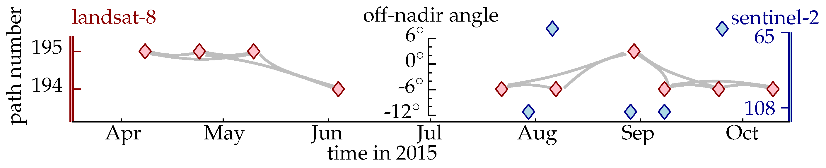
4. Data and Study Areas

The methodology given above can be used for several application scenarios. Within the present study we highlight three different case studies. All studies have varying objectives in order to show the wide range of possibilities of applying our methodology, but they also show the diversity of challenges that occur for mountain glaciers in relation to fast-flowing and big outlet glaciers.

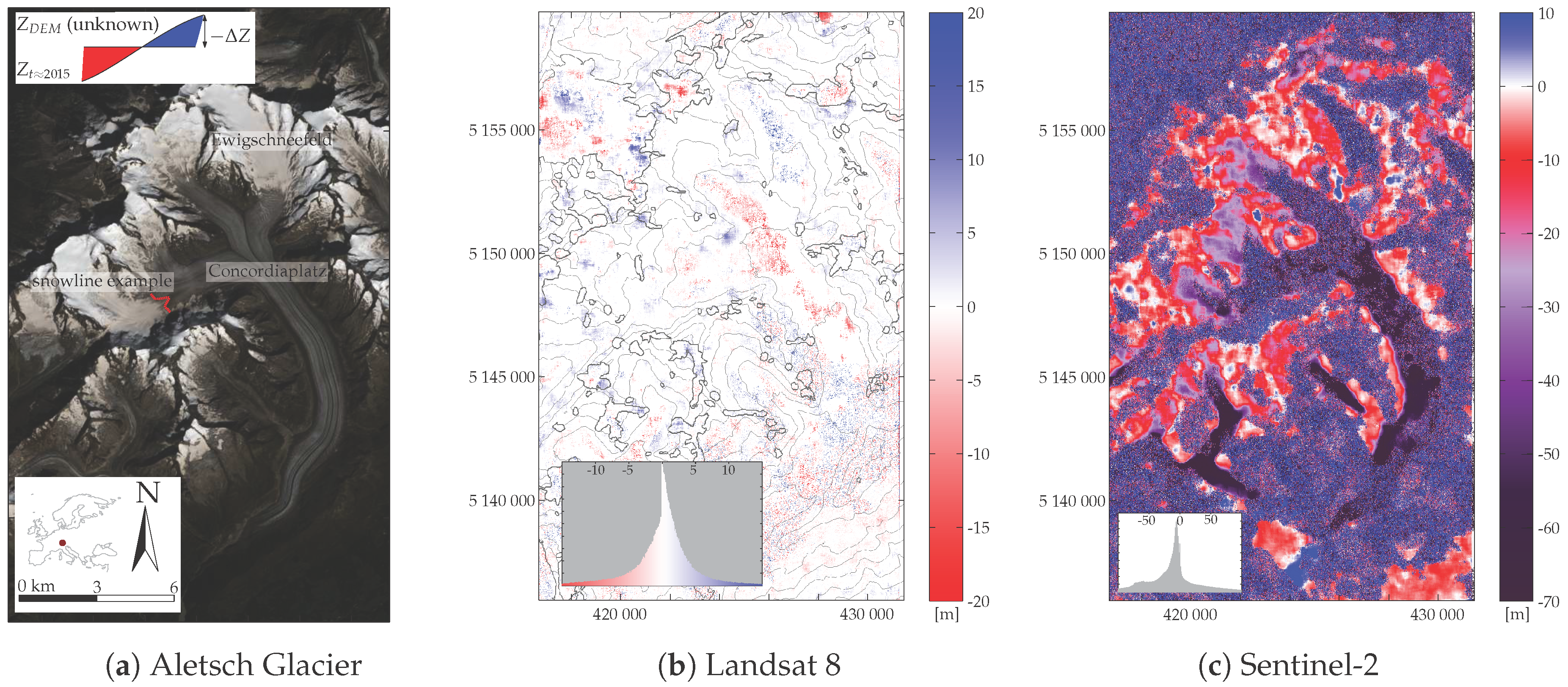
4.1. Aletsch, Switzerland

At 83 km² the Grosser Aletsch Glacier is the largest glacier in the European Alps (Figure 4a). Since 1881 the net balance of this glacier has been negative. This resulted in a retreat of the front and a reduction of elevation at its snout, which can be up to four meters per year [39].

In this study, we use data from Landsat 8 and Sentinel-2 (see Figure A1 in the Appendix for a baseline plot and a list of individual scenes). Data from both satellites are freely available and are therefore popular. Landsat 8 has a same-orbit revisit time of 16 days, while Sentinel-2 will consist of two satellites forming a constellation with a revisit time of 5 days. When imagery from different looking angles is used, the chance of acquiring cloud-free imagery increases, especially for Sentinel-2 where the wide looking angle results in overlap between orbits, and greatly increases as orbits converge to the poles, see Figure 2 in [20]. However, the wide looking angle results in more cross-track offset. In addition, the Aletsch Glacier is surrounded by steep topography and has an icefall, making it a representative case for studying high mountain glaciers. For the assessment of our estimated vertical DEM offsets we use a no-voids filled version of SRTM.

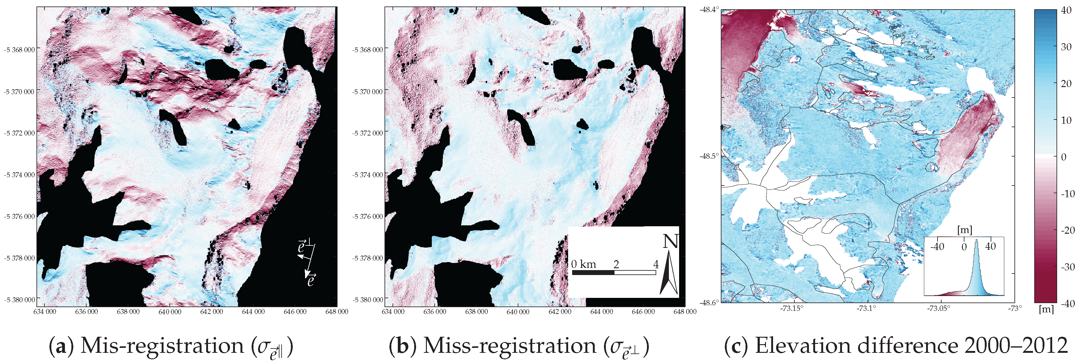
4.2. Oriental, Patagonia

Oriental Glacier (Figure 5) is situated at the northeastern side of the southern Patagonian icefield. Most outlet glaciers on the western side of the icefield drain into fjords, while eastern glaciers often terminate in freshwater lakes. Oriental Glacier is physically, but not hydrologically connected to the icefield. The glacier has a wide accumulation area and below an icefall it flows northwards where it funnels and elongates until it terminates into a lake. Another glacier branch, called Mellizos Sur, flows southwards and is also lake-terminating. The frontal positions of both snouts have been retreating slowly over the last decades. Its areal extent has decreased by 1% per decade for the last three decades [40]. In 1986 the area of the glacier was 73.68 km². Generally, most glaciers within this area are retreating [41], and the Oriental is no exception [42], though minor in a regional perspective [40]. Together with the ancillary retreat, an elevation loss is observed over large parts of the icefield since 2000 [43]. In the three decades prior to 2000, significant lowering is observed at most snouts of the icefield [44]. For the Oriental glacier, the ice loss over 1975–2000 is estimated to be 0.03 km³.

For this case study we want to investigate if it is possible to detect elevation differences over a time span of a decade through a temporal variation in orthoprojection offsets. Therefore we use data from the beginning of the Landsat 7 and 8 missions, as illustrated in Figure A2 and listed in the Appendix. Archive imagery was selected that was cloud free, or with only a limited amount of obstruction by clouds. The elevation models used to assess our estimated DEM offsets are a SRTM DEM from 2000 and a TandDEM-X DEM from 2012.

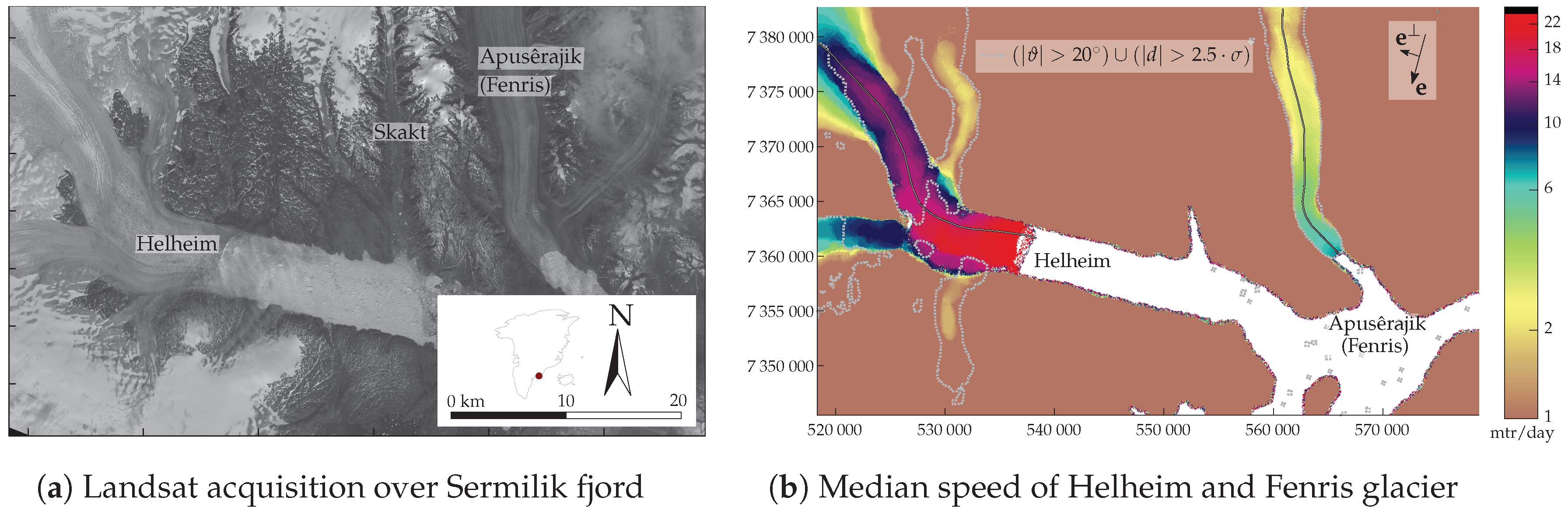
4.3. Helheim, Greenland

Helheim Glacier (66.5°N, 38°W) is the third largest of the many outlets of the Greenland ice sheet. The Helheim Glacier drains into the Sermilik fjord, together with Fenris and Midgård glaciers.

In the previous decade, an increase in velocity was observed for Helheim between 2000 and 2005 [45]. This was accompanied by a drawdown of the surface. Because surface melt is not able to account for all measured elevation loss, ice dynamics must have played a prominent role [46]. Within the period of 2000–2005, the ice front seemed to be at or near floatation. In this unstable situation the front could advance and retreat several kilometres within a season [47]. The other glacier within this study site is Fenris Glacier, which is also a marine terminating glacier. It transports ice from the Greenland ice sheet through a narrow fjord and has less seasonal front variations compared to the Helheim Glacier. Between 1972–2011 the front of Fenris Glacier has retreated 2.6 km [48].

These two glaciers appear to represent two different types of outlets. Helheim Glacier is an unstable case, which is heavily effected by frontal ablation and is close to floatation, while Fenris Glacier might be less sensitive due to its narrow outlet. Assessing the weekly velocity change might reveal patterns which occur at these time scales. Up to now, it was not possible to assess the contribution of melt-water triggered speed-up [45]. However, by increasing the number of satellite images included into the image matching, as is the aim of this study, it might be possible to gain more insight into such processes.

5. Results

The methodology as described above is applied to the three different case studies, each highlighting a different application of information retrieval. In the first case, the Aletsch Glacier, the orthorectification error is estimated for two different satellites, Landsat 8 and Sentinel-2. This is of technical interest towards homogenization of data from both missions, highlighting the processing pipeline abilities and can be seen as a quality indicator of the underlying topographic data sources. In the second case, the Oriental Glacier, the orthorectification offsets are assessed over time in order to evaluate if elevation changes over glaciers can be extracted. This is to show the capabilities of our methodology and can also be seen as an assessment of the relative georeferencing abilities of the processing pipeline. In the last case, Helheim Glacier, the temporal sampling of velocity measurements over an outlet is increased. Here the processing is without complicated estimations of the orthorectification offsets. This last case study mimics the use for more general geophysical purposes, where one is interested in the temporal flow dynamics of glaciers. Due to its simplicity this last case study is the most relevant methodology for operational use and bulk processing.

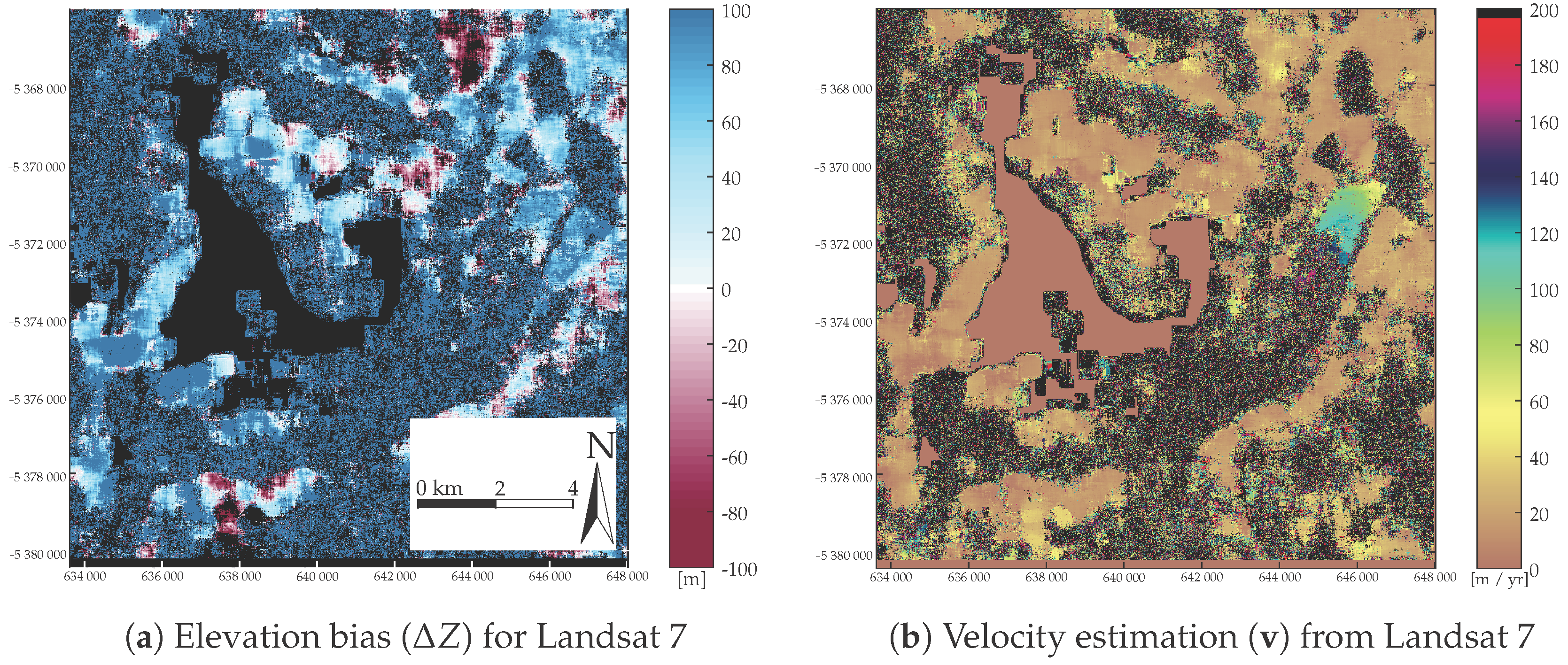
5.1. DEM Bias (Aletsch Glacier)

Over Aletsch Glacier (see Figure 4a) the estimation of single-time DEM bias, reconstructed from lateral orthorectification offsets between neighboring orbits following Equations (11) and (12) from Landsat 8 and Sentinel-2A imagery is illustrated in Figure 4b,c. In total, 7 and 10 image triplets were used for the Landsat 8 and Sentinel-2 case, respectively. For Landsat 8, as shown in Figure 4b, the SRTM DEM dataset is also included. The SRTM contours (with 250 m interval) are shown, and the thicker lines indicate void areas. Within the void areas, patches of significant vertical bias are located at mountain tops. However, patches of strong bias also occur on other non-glacial terrain. The DEM bias pattern shows a consistent signal of positive values on the lower tongue and upper north-eastern part (the Ewigschneefeld, see Figure 4a) (i.e., the DEM used for orthorectification is lower than the terrain at image acquisition). A clear transition is present at the ice-fall where the snowline is situated. The elevation bias in the middle glacier part (around Concordiaplatz and below) might be due to the negative net mass balance and according elevation loss. However, the signal in the upper part (Ewigschneefeld) does not correspond with the expected spatial distribution of the mass balance, as in [39]. Presumably, an elevation model rooted from the SRTM mission is used for Landsat 8 orthorectification. SRTM radar waves penetrate into the snow pack and the resulting backscatter phase center might be situated several meters within the snowpack [49,50,51]. This effect would have led to a too low reference DEM, not (yet) compensated by actual surface elevation loss. In the lower part of the glacier, the estimates are scattered and fluctuate. This is rooted in the unfortunate timing for this case, as in spring the snowline is in close proximity, hence visual surface features are not stable. For the other imagery which was acquired in summer and autumn, the scenes have partial cloud cover over the lower glacier snout. Consequently, only a limited sample size produces these estimates and should therefore be interpreted with caution. In theory, also a massive paraglacial landslide ongoing directly adjacent to the orographic left side of the glacier tongue [52] could have influenced glacier elevation and/or flow regime.

The estimated terrain bias for the Sentinel-2A data is illustrated in Figure 4c. Rough speckle surrounds the glacier and corresponds to clouds, present within the imagery. In addition, speckle is present on the accumulation areas, as a migrating snowline corrupts the stability of visual appearance in these areas. A negative bias seems to be present over the full dataset (note the different colour scale in Figure 4c displaying almost exclusively negative values compared to Figure 4b), and overall the magnitude of the bias is larger by one order of magnitude compared to the Landsat 8 data. Within the histogram a second peak is observable at around −60 m, largely corresponding to the lower part of the glaciers. For the icefall above the central part of the glacier, called Concordiaplatz, an opposite signal can be observed. This reversal of the bias might be due to the use of a lower resolution elevation model. This covers the lower frequencies of the terrain, but is not able to represent finer transitions [53]. The suspicion of a low resolution elevation model is also detected for Sentinel-2 in a Norwegian case study [20]. Unfortunately, these artifacts are of serious concern for the optimal exploitation of Sentinel-2 data for high mountain glacier studies.

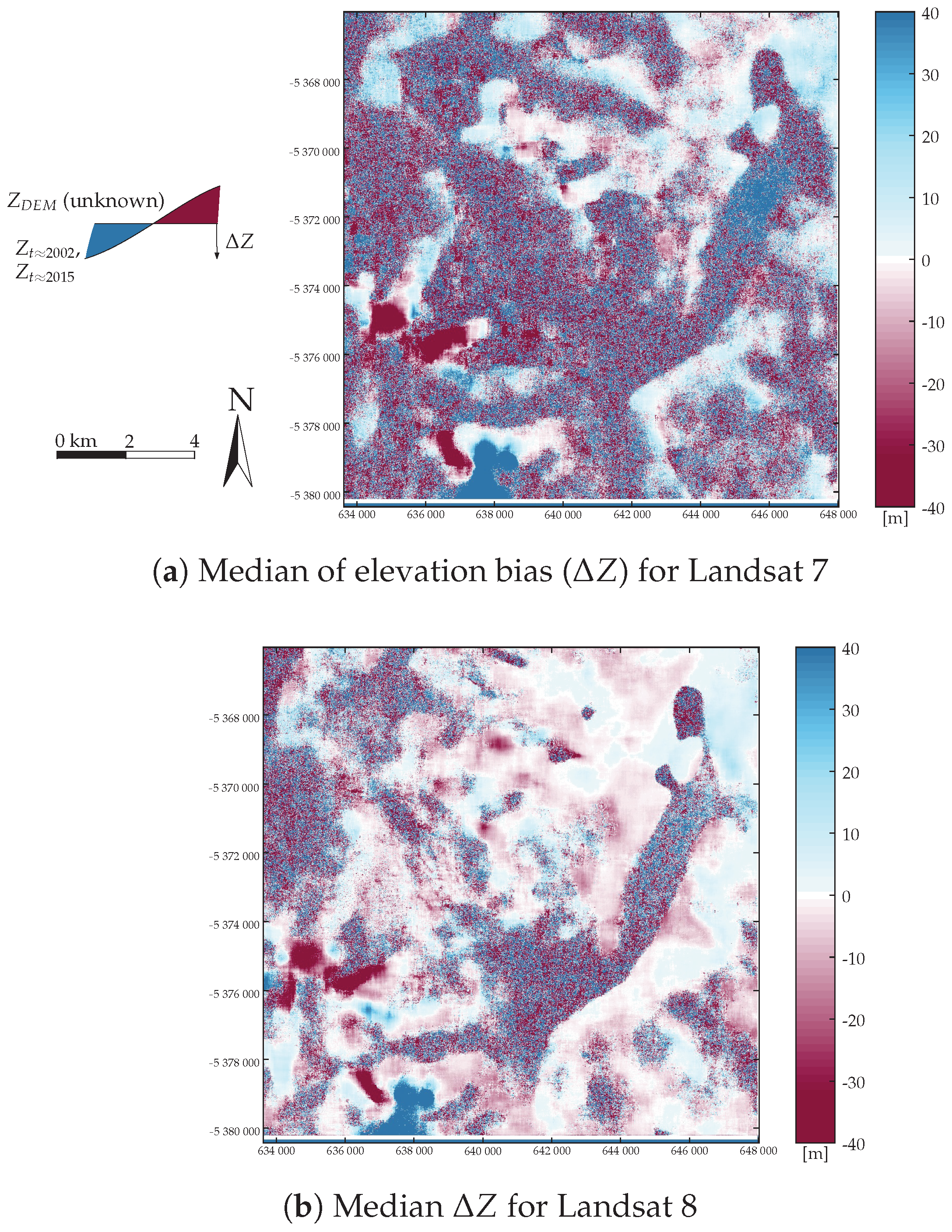
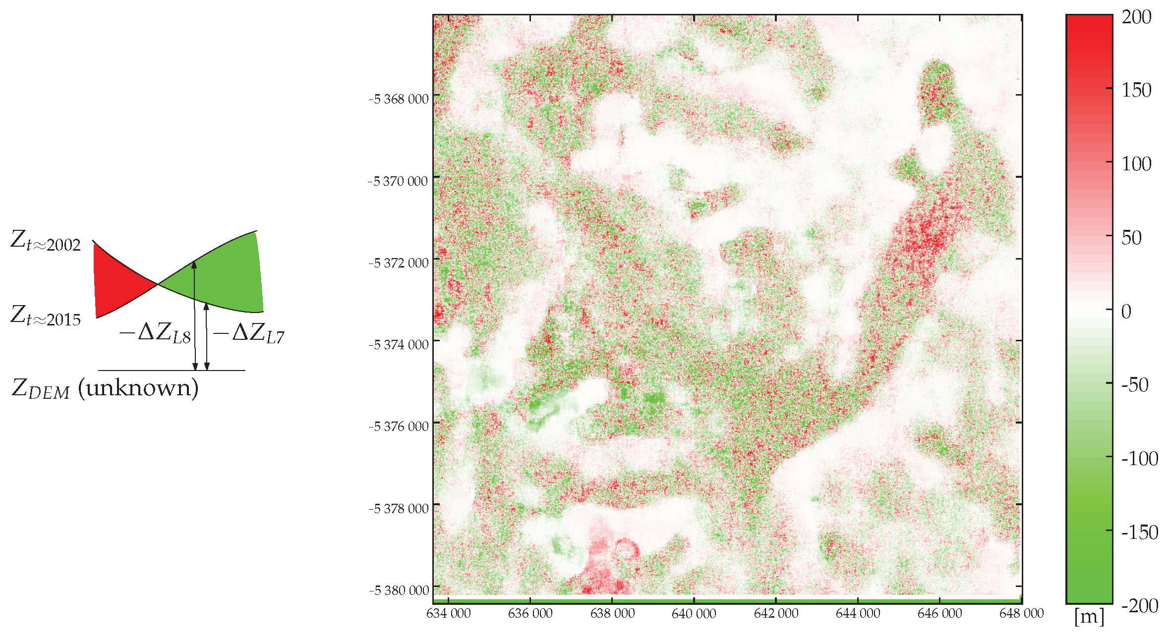
5.2. Elevation Change over Time (Oriental Glacier)

In this second application, we test whether orthorectification offsets from different times could be used to roughly identify actual elevation changes over time. Here, we compare orthorectification offsets from Landsat 7 data from the early 2000s to those in Landsat 8 data from the mid 2010s. The estimation of orthorectification errors and velocity is based on matches from a collection of different images. Finding an optimal combination of imagery to match is challenging, firstly, because glacier displacement estimation relies on visual similarity. However, within an imagewindow different features contribute to the pattern. Such features have different life spans, and can be short lived or obstructed. Secondly, the movements need to be statistically significant in order to be above the noise level of the displacement estimation. Consequently, all combinations between imagery are used in this study, as individual triplets contain no-data values or outliers, but these might be populated by other combinations. For example, the elevation difference estimation for a single triplet is illustrated in Figure 6.

Because of the long timespan of a year for the specific image pairs matched, many features are de-correlated in the middle part of the glacier. In the upper part of the glacier the saturation of the bands results in voids (black) or in very small displacements. Nonetheless, the snout seems to exhibit a consistent velocity estimate. Because the relative intersection angle is small (≈9° see Figure 5), the elevation estimation fluctuates heavily. Patches are observable, which might show co-registration and ortho-rectification errors, but these errors are within the same order as the noise due to the bad viewing geometry.

In order to exceed the noise level, the elevation bias and velocity field is estimated for multiple image triplets; 286 combinations for Landsat 7 and 120 for Landsat 8. Because every scene can be hampered by clouds, and because of co-registration errors and different temporal feature degradations, the single estimates are very noisy. However, the co-registration errors can be assumed to be random, as well as the cloud cover to some extent. As the sampling has different temporal baselines, different features within the image windows are used to estimate the displacements. Consequently, when the median of all estimates is taken the outliers and noise are diminished, revealing a more accurate and reliable elevation bias than if only single triplets are used as in Figure 6. For both sensors, Landsat 7 and 8, the median of the elevation estimations is illustrated in Figure 7a,b. For Landsat 7 the most extreme outliers correspond to the mountain tops, such as Cerro Steffen (the purple square in Figure 5), and at icefalls. This might be due to the coarse resolution of the elevation model used for orthorectifying the Landsat data [53]. A clear pattern at the snout is observable as well, with a bias of several meters. For the Landsat 8 elevation bias estimation the pattern is more clearly observable. The height of glaciated terrain is larger by our method compared to the orthorectification DEM, while rock outcrops and terrain features are lower. However, the clear difference pattern of outliers on mountain tops found for the Landsat 7 data is not present in our Landsat 8-based reconstruction. Furthermore, the accumulation area of the glacier exhibits better estimates, which is due to the superior radiometric range of the Landsat 8 instrument.

When the elevation bias estimates from both the Landsat 7 and 8 data (i.e., Figure 7a,b) are differenced, topographic change should become observable. This is illustrated in Figure 8. Apart from the speckle, due to noise, some coherent elevation change patterns are observable, firstly on the mountain tops, but also the snout of the Oriental Glacier has clearly changed in elevation. Because the inaccuracy of the matching is strongly exaggerated through error propagation in combination with the small intersection angle, one should focus more on the trend pattern than its absolute numbers. Hence, only the sign of the change can be seen as significant.

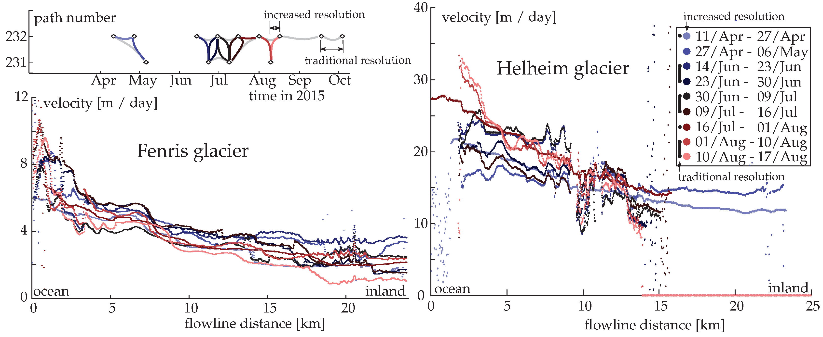
5.3. Increased Temporal Resolution (Helheim Glacier)

In this third and final test we eliminate orthorectification offsets between satellite images from different orbits in order to arrive at a bias-free velocity time-series with higher temporal resolution than is achievable from repeat orbits only.

An Landsat 8 acquisition over Sermilik fjord, and its extracted base-line velocity are illustrated in Figure 9a,b. The time-series of Helheim and Fenris glaciers are illustrated in Figure 10. The median velocity is calculated from matches which have a signal-to-noise ratio (SNR) higher than 10. Furthermore, only displacements which where higher than 2.5 times the relative distance ($\left|\mathbf{d}\right|/{\sigma }_d$, see Figure 3) where taken into consideration for projecting the raw estimated displacement onto the assumed constant flow direction. For both glaciers in early spring and late autumn, a steady background velocity seems to be present before a speed-up occurs in July. For Fenris Glacier this speed-up is even observed far inland, but seems short lived. At the Helheim outlet a more complicated signal is present. Here, the speed-up is of a factor of four times accelerated from the lowest speeds in late/early winter, but its effect is less visible further upstream. In addition, later in the season an increase of speed near the terminus is observed, which relates to a longitudinal extension of the ice, creating more fractures/crevasses, connected to a less stable snout.

In both speed plots all projections are illustrated, and the filter as illustrated in Figure 3 is not applied for the relative flow angle (ϑ). As can be seen in the speed plots, outliers occur at specific places. For Helheim Glacier the scatter occurs where the outlet makes a turn and the displacement is in the same direction as the across-track direction (${\mathbf{e}}^{\perp }$), which leads to strong amplification of matching inaccuracy in our projection process. Scatter occurs on Fenris Glacier as well, but this is due to the flowline sampling displacement estimates within the fjord water and not on the glacial ice.

6. Discussion

As demonstrated, our methodology is capable of assessing the geometric quality of orthorectified Earth observation images. However, the implementation has also its limitations. The bearing of glacier flow is the most confining parameter. If the glacier flow is in the across-track direction of the observing platform, the system of equations is ill-posed. Because most Earth observation systems follow the same near-polar orbit, specific parts of a glacier will give poor estimates for all available data. For example, velocities over the sharp bend within the Helheim Glacier can only be estimated using the traditional repeat-orbit method, as well as over the icefall behind the tongue of the Oriental Glacier. In future work, it might be possible to constrain the estimates by including the property of ice to be incompressible into the system of equations. However, this complicates the estimation structure, from a straight forward individual scheme to an iterative locally dependent structure. Furthermore, it will neglect the possibility for ice to extend in the vertical direction. Optical satellites/instruments in an International Space Station (ISS) orbit might be able to constrain the geometry, however are not able to cover polar glaciers.

Furthermore, the geometry of the acquisition matters. Most affected by orthorectification bias are acquisitions with a wide off-nadir angle, through its wide viewing (e.g., Sentinel-2) or its steering capabilities (e.g., ASTER, SPOT). With such systems the combination of intersection angle and resolution is sufficient to estimate a significant displacement. For the Landsat case, the results are more noisy. This is partly due to the narrow intersection angle between acquisitions from different orbits, but also the assumption of perfect georeferencing does play a role. Stable and flat terrain are needed to find such overall lateral displacements. However, if such scene specific parameters are included, the system of equations becomes ill-conditioned.

A second subject of concern is the warping applied to the Landsat imagery [7]. This causes local distortions, and might be the reason why not every part of the bias pattern can be explained. However, the difference between Landsat 7 and 8 on Oriental Glacier is not solely dependent on the warping. It is a combination of warping and absolute orientation error, as the absolute orientation does produce a terrain-dependent signal [54]. Untangling these effects is challenging as both errors are directly related to topography. Fortunately, for the case of the Oriental Glacier we do have elevation data of SRTM, which were acquired in austral summer. In February 2000, it was exceptionally warm, thus radar penetration was minimal. Furthermore, an elevation model from the recent Deutsches Zentrum für Luft- und Raumfahrt (DLR) TanDEM-X mission gives us an opportunity to assess our estimate of glacier thickness change. By replicating the DLR TanDEM-X DEM and applying a planar shift to its copy, a georeferencing error can be simulated. Both components; the one in the direction of the flight line and the one perpendicular to it, are illustrated in Figure 11a,b, respectively. The patterns of these components do not seem to be observable in our estimates. This implies that the distribution of geo-referencing errors could be stochastic. The elevation difference between both the 2000 SRTM and 2012 TanDEM-X elevation models is illustrated in Figure 11c. Here a clear signal of an elevation loss on the snout can be seen, which does relate to our estimates (Figure 8) in both spatial distribution and magnitude of bias/elevation change. Unfortunately, the elevation models have no elevation information on the mountain tops because of interferometric phase unwrapping problems.

Our estimation model used in the Aletsch and Oriental case studies relies on constant speed. However, some dynamics might be present in the flow regime, which are not formulated in the model. Consequently, any deviation will propagate into the elevation bias estimate, which is already sensitive due to its slim intersection angle. Hence in this study we used short time ranges within a year or up to three years. Furthermore, a variable speed model can cause overfitting of the data, resulting in velocities estimations with different flow directions. This is especially the case when the base-line is close to perpendicular in space-time. On the other hand, because of these potential variations in speed the simple model of constant speed over the study period was not executed on the far more dynamic tide water Helheim Glacier.

7. Conclusions

This study introduces a sensor-independent method to analyse DEM-induced errors in repeat orthorectified optical data, even when terrain might be moving. The framework is built around simple ordinary least squares, hence the estimation is extendable to various sensors and terrain movement types. In addition, an efficient and robust manner of triplet matching, instead of traditional pairwise matching, is introduced. Because the full spectrum of candidate displacements is used in triplet matching, the triangle closure constraint is able to identify secondary correlation peaks as valid, which would otherwise be disregarded in traditional pairwise matching, where the highest correlation value is considered the valid match. The implementation of the triangle closure constraint is built upon simple convolution. It can be implemented both in the spatial and the frequency domain. The robustness of the triplet matching method is enhanced through the multiplication of the displacement scores. A benefit is achieved when implementing the method in the frequency domain, as such displacement estimates produce only a limited amount of peaks that stand out sharp and clearly, hence displacement estimates should be aligned otherwise the signal will be damped. In the spatial domain, such peaks are mostly smoother, and have lower signal to noise ratios, hence the geometric constraint through multiplication will stand out less.

Our methodology of exploiting orthorectification offsets is demonstrated using three different case studies. We were able to identify artifacts in the orthorectification processes, and show elevation changes over time related to glacier change. Furthermore, we were able to compare Landsat 8 and Sentinel-2 products, and find an order of magnitude larger orthorectification errors for Sentinel-2. However, these differences can solely be attributed to the reference model, hence when a better DEM is used for Sentinel-2 the quality might enhance accordingly. Lastly, we introduced a mapping routine, which bypasses the elevation bias estimate and directly produces velocity estimates using imagery from different orbits, eventually leading to elevation bias-free velocity measurements with higher temporal resolution than can be achieved using repeat-pass data only.

The ordinary least squares framework given in this study is a diverse structure to build upon, and can be exploited in various other ways. For example, if more acquisitions are taken into the system of equations, a network can be built. This opens up the possibility to apply statistical tests and data-snooping, due to an increase in redundancy. Furthermore, our framework has the ability to propagate errors, when normally distributed, and thus estimate the deviation of estimated parameters. Such procedures become more and more valuable with the increasing availability of optical satellite data, such as from the recently successful launched Sentinel-2B. In principle, our method is also applicable to SAR data, but inter-orbit image matching might be complicated by the oblique viewing angle and active acquisition nature of SAR that make the appearance of ground features likely more variable.

This study underlines that the orthorectification procedure is an essential aspect of data quality of remote sensing image products. When the underlying elevation model is of sufficient quality, across-track analyses are possible and have the potential to increase information retrieval considerably and enhance homogenization between data from different missions such as Landsat and Sentinel-2.

References

1. Kääb, A.; Leprince, S. Motion detection using near-simultaneous satellite acquisitions. Remote Sens. Environ. 2014, 154, 164–179. [Google Scholar] [CrossRef] [Green Version]
2. Van der Veen, C. Fundamentals of Glacier Dynamics; CRC Press: Boca Raton, FL, USA, 2013. [Google Scholar]
3. Nick, F.; Van der Veen, C.; Vieli, A.; Benn, D. A physically based calving model applied to marine outlet glaciers and implications for the glacier dynamics. J. Glaciol. 2010, 56, 781–794. [Google Scholar] [CrossRef] [Green Version]
4. Fahnestock, M.; Scambos, T.; Moon, T.; Gardner, A.; Haran, T.; Klinger, M. Rapid large-area mapping of ice flow using Landsat 8. Remote Sens. Environ. 2016, 185, 84–94. [Google Scholar] [CrossRef]
5. Dehecq, A.; Gourmelen, N.; Trouve, E. Deriving large-scale glacier velocities from a complete satellite archive: Application to the Pamir–Karakoram–Himalaya. Remote Sens. Environ. 2015, 162, 55–66. [Google Scholar] [CrossRef]
6. Rosenau, R.; Scheinert, M.; Dietrich, R. A processing system to monitor Greenland outlet glacier velocity variations at decadal and seasonal time scales utilizing the Landsat imagery. Remote Sens. Environ. 2015, 169, 1–19. [Google Scholar] [CrossRef]
7. Gao, F.; Masek, J.; Wolfe, R. Automated registration and orthorectification package for Landsat and Landsat-like data processing. J. Appl. Remote Sens. 2009, 3, 033515. [Google Scholar]
8. Bian, J.H.; Li, A.N.; Jin, H.A.; Lei, G.B.; Huang, C.Q.; Li, M.X. Auto-registration and orthorecification algorithm for the time series HJ-1A/B CCD images. J. Mt. Sci. 2013, 10, 754–767. [Google Scholar] [CrossRef]
9. Devaraj, C.; Shah, C. Automated geometric correction of Landsat MSS L1G imagery. IEEE Geosci. Remote Sens. Lett. 2014, 11, 347–351. [Google Scholar] [CrossRef]
10. Devaraj, C.; Shah, C. Automated geometric correction of multispectral images from High Resolution CCD Camera (HRCC) on-board CBERS-2 and CBERS-2B. ISPRS J. Photogramm. Remote Sens. 2014, 89, 13–24. [Google Scholar] [CrossRef]
11. Altena, B.; Kääb, A.; Nuth, C. Robust glacier displacements using knowledge-based image matching. In Proceedings of the 2015 8th International Workshop on the Analysis of Multitemporal Remote Sensing Images (Multi-Temp), Annecy, France, 22–24 July 2015; pp. 1–4.
12. Stumpf, A.; Malet, J.P.; Delacourt, C. Correlation of satellite image time-series for the detection and monitoring of slow-moving landslides. Remote Sens. Environ. 2017, 189, 40–55. [Google Scholar] [CrossRef]
13. Jeong, S.; Howat, I.M.; Ahn, Y. Improved multiple matching method for observing glacier motion with repeat image feature tracking. IEEE Trans. Geosci. Remote Sens. 2017, 55, 2431–2441. [Google Scholar] [CrossRef]
14. Moons, T.; Van Gool, L.; Vergauwen, M. 3D Reconstruction from Multiple Images, Part 1: Principles; Foundations and Trends® in Computer Graphics and Vision; Now Publishers Inc.: Breda, The Netherlands, 2009. [Google Scholar]
15. Tucker, C.; Grant, D.; Dykstra, J. NASAs global orthorectified Landsat data set. Photogramm. Eng. Remote Sens. 2004, 70, 313–322. [Google Scholar] [CrossRef]
16. Storey, J.; Strande, D.; Hayes, R.; Meyerink, A.; Labahn, S.; Lacasse, J. Landsat 7 Image Assessment System (IAS) Geometric Algorithm Theoretical Basis Document; Technical Report; USGS: Reston, VA, USA, 2006.
17. Chen, L.C.; Lee, L.H. Rigorous generation of digital orthophotos from SPOT images. Photogramm. Eng. Remote Sens. 1993, 59, 655–661. [Google Scholar]
18. Sun, G.; Ranson, K.; Kharuk, V.; Kovacs, K. Validation of surface height from shuttle radar topography mission using shuttle laser altimeter. Remote Sens. Environ. 2003, 88, 401–411. [Google Scholar] [CrossRef]
19. Kääb, A. Remote Sensing of Mountain Glaciers and Permafrost Creep; Geographisches Institut der Universität Zürich: Zürich, Switzerland, 2005. [Google Scholar]
20. Kääb, A.; Winsvold, S.; Altena, B.; Nuth, C.; Nagler, T.; Wuite, J. Glacier Remote Sensing using Sentinel-2. Part I: Radiometric and Geometric Performance, Application to Ice Velocity, and Comparison to Landsat 8. Remote Sens. 2016, 8, 598. [Google Scholar] [CrossRef]
21. Teunissen, P. Adjustment Theory. An Introduction, Series on Mathematical Geodesy and Positioning; VSSD: Delft, The Netherlands, 2003. [Google Scholar]
22. Barron, J.; Fleet, D.; Beauchemin, S. Performance of optical flow techniques. Int. J. Comput. Vis. 1994, 12, 43–77. [Google Scholar] [CrossRef]
23. Baker, S.; Scharstein, D.; Lewis, J.; Roth, S.; Black, M.; Szeliski, R. A database and evaluation methodology for optical flow. Int. J. Comput. Vis. 2011, 92, 1–31. [Google Scholar] [CrossRef]
24. Vogel, C.; Bauder, A.; Schindler, K. Optical Flow for Glacier Motion Estimation. In Proceedings of the 22nd ISPRS Congress, Melbourne, Australia, 25 August–1 September 2012.
25. Altena, B.; Kääb, A. Weekly glacier flow estimation from dense satellite time series using adapted optical flow technology. Front. Earth Sci. 2017. in review. [Google Scholar]
26. Tuytelaars, T.; Mikolajczyk, K. Local invariant feature detectors: A survey. Found. Trends Comput. Gr. Visi. 2008, 3, 177–280. [Google Scholar] [CrossRef] [Green Version]
27. Tola, E.; Lepetit, V.; Fua, P. Daisy: An efficient dense descriptor applied to wide-baseline stereo. IEEE Trans. Pattern Anal. Mach. Intell. 2010, 32, 815–830. [Google Scholar] [CrossRef] [PubMed]
28. Kokkinos, I.; Bronstein, M.; Yuille, A. Dense Scale Invariant Descriptors for Images and Surfaces; INRIA: Paris, France, 2012. [Google Scholar]
29. Muye, N.; Chunxia, Z.; Tingting, L. Derivation of ice-flow of Polar Record Glacier using an improved NCC algorithm. Chin. J. Polar Res. 2016, 28, 243–249. [Google Scholar]
30. Bindschadler, R.; Scambos, T. Satellite-image-derived velocity field of an Antarctic ice stream. Science 1991, 252, 242. [Google Scholar] [CrossRef] [PubMed]
31. Scambos, T.; Dutkiewicz, M.; Wilson, J.; Bindschadler, R. Application of image cross-correlation to the measurement of glacier velocity using satellite image data. Remote Sens. Environ. 1992, 42, 177–186. [Google Scholar] [CrossRef]
32. Kääb, A.; Vollmer, M. Surface geometry, thickness changes and flow fields on creeping mountain permafrost: Automatic extraction by digital image analysis. Permafr. Periglac. Process. 2000, 11, 315–326. [Google Scholar] [CrossRef]
33. Heid, T.; Kääb, A. Evaluation of existing image matching methods for deriving glacier surface displacements globally from optical satellite imagery. Remote Sens. Environ. 2012, 118, 339–355. [Google Scholar] [CrossRef]
34. Ahn, Y.; Howat, I. Efficient automated glacier surface velocity measurement from repeat images using multi-image/multichip and null exclusion feature tracking. IEEE Trans. Geosci. Remote Sens. 2011, 49, 2838–2846. [Google Scholar]
35. Goshtasby, A. Image Registration: Principles, Tools and Methods; Advances in Computer Vision and Pattern Recognition; Springer: Berlin, Germany, 2012. [Google Scholar]
36. Erten, E. Glacier velocity estimation by means of a polarimetric similarity measure. IEEE Trans. Geosci. Remote Sens. 2013, 51, 3319–3327. [Google Scholar] [CrossRef]
37. Rolstad, C.; Amlien, J.; Hagen, J.O.; Lundén, B. Visible and near-infrared digital images for determination of ice velocities and surface elevation during a surge on Osbornebreen, a tidewater glacier in Svalbard. Ann. Glaciol. 1997, 24, 255–261. [Google Scholar] [CrossRef]
38. Hart, D. PIV error correction. Exp. Fluids 2000, 29, 13–22. [Google Scholar] [CrossRef]
39. Bauder, A.; Funk, M.; Huss, M. Ice-volume changes of selected glaciers in the Swiss Alps since the end of the 19th century. Ann. Glaciol. 2007, 46, 145–149. [Google Scholar] [CrossRef]
40. White, A.; Copland, L. Decadal-scale variations in glacier area changes across the Southern Patagonian Icefield since the 1970s. Arct. Antarct. Alp. Res. 2015, 47, 147–167. [Google Scholar] [CrossRef]
41. Lopez, P.; Chevallier, P.; Favier, V.; Pouyaud, B.; Ordenes, F.; Oerlemans, J. A regional view of fluctuations in glacier length in southern South America. Glob. Planet. Chang. 2010, 71, 85–108. [Google Scholar] [CrossRef]
42. Davies, B.; Glasser, N. Accelerating shrinkage of Patagonian glaciers from the Little Ice Age (AD 1870) to 2011. J. Glaciol. 2012, 58, 1063–1084. [Google Scholar] [CrossRef]
43. Willis, M.; Melkonian, A.; Pritchard, M.; Rivera, A. Ice loss from the Southern Patagonian Ice Field, South America, between 2000 and 2012. Geophys. Res. Lett. 2012, 39, L17501. [Google Scholar] [CrossRef]
44. Rignot, E.; Rivera, A.; Casassa, G. Contribution of the Patagonia Icefields of South America to sea level rise. Science 2003, 302, 434–437. [Google Scholar] [CrossRef] [PubMed]
45. Howat, I.; Joughin, I.; Tulaczyk, S.; Gogineni, S. Rapid retreat and acceleration of Helheim Glacier, east Greenland. Geophys. Res. Lett. 2005. [Google Scholar] [CrossRef]
46. Stearns, L.; Hamilton, G. Rapid volume loss from two East Greenland outlet glaciers quantified using repeat stereo satellite imagery. Geophys. Res. Lett. 2007. [Google Scholar] [CrossRef]
47. Joughin, I.; Howat, I.; Alley, R.; Ekström, G.; Fahnestock, M.; Moon, T.; Nettles, M.; Truffer, M.; Tsai, V. Ice-front variation and tidewater behavior on Helheim and Kangerdlugssuaq Glaciers, Greenland. J. Geophys. Res. Earth Surf. 2008. [Google Scholar] [CrossRef]
48. Mernild, S.; Malmros, J.; Yde, J.; Knudsen, N. Multi-decadal marine-and land-terminating glacier recession in the Ammassalik region, southeast Greenland. Cryosphere 2012, 6, 625–639. [Google Scholar] [CrossRef] [Green Version]
49. Rignot, E.; Echelmeyer, K.; Krabill, W. Penetration depth of interferometric synthetic-aperture radar signals in snow and ice. Geophys. Res. Lett. 2001, 28, 3501–3504. [Google Scholar] [CrossRef]
50. Berthier, E.; Arnaud, Y.; Vincent, C.; Remy, F. Biases of SRTM in high-mountain areas: Implications for the monitoring of glacier volume changes. Geophys. Res. Lett. 2006. [Google Scholar] [CrossRef]
51. Kääb, A.; Berthier, E.; Nuth, C.; Gardelle, J.; Arnaud, Y. Contrasting patterns of early twenty-first-century glacier mass change in the Himalayas. Nature 2012, 488, 495–498. [Google Scholar] [CrossRef] [PubMed]
52. Strozzi, T.; Delaloye, R.; Kääb, A.; Ambrosi, C.; Perruchoud, E.; Wegmüller, U. Combined observations of rock mass movements using satellite SAR interferometry, differential GPS, airborne digital photogrammetry, and airborne photography interpretation. J. Geophys. Res. Earth Surf. 2010. [Google Scholar] [CrossRef]
53. Paul, F. Calculation of glacier elevation changes with SRTM: Is there an elevation-dependent bias? J. Glaciol. 2008, 54, 945–946. [Google Scholar] [CrossRef] [Green Version]
54. Nuth, C.; Kääb, A. Co-registration and bias corrections of satellite elevation data sets for quantifying glacier thickness change. Cryosphere 2011, 5, 271–290. [Google Scholar] [CrossRef]
Figure 1. Schematic drawing of orthorectification offsets due to DEM errors in respect to different viewing acquisitions.
Remotesensing 09 00300 g001
Figure 2. Planar view of components for the displacement projection. The estimated displacement ( d ) is the raw image displacement estimation from an image pair from different viewing angles. The initial displacement ( d ˜ ) is an assumed correct terrain movement that can be derived from a repeat-orbit pair (i.e., with minimal orthorectification offsets), or auxiliary data. The key condition of this initial displacement is that its direction sufficiently approximates the real terrain movement, not necessarily its correct magnitude. This assumption takes into account that for instance glaciers will typically change their flow magnitude much faster and stronger than their flow direction. The projected displacement ( d ^ ) is then the final estimation of terrain movement, with orthorectification offsets removed.
Remotesensing 09 00300 g002
Figure 3. Illustration of the sensitivity of the projection method. In dashed light blue the accuracy of matching is illustrated ( σ d ) on the displacement vector ( d ). The dark blue vector is the a priori displacement ( d ˜ ) from a pair with the same viewing angle or from auxiliary data. Finally, the dashed gray line illustrates the across-track looking direction, or epipolar line ( e ) and relative angle (ϑ). In this case only the upper left situation is a valid projection example.
Remotesensing 09 00300 g003
Figure 4. Estimation of terrain bias between surface elevation (Zt) during acquisition and DEM (ZDEM) used for orthorectification (−ΔZ in Figure 1) for different sensors. When the estimation is negative the reference DEM used for orthorectification is higher than the real surface at image acquisition. The histograms in the lower left corners illustrate the distributions of the estimated terrain bias.
Remotesensing 09 00300 g004
Figure 5. Landsat acquisition over Oriental Glacier, iso-lines indicate the off-nadir looking angle in degrees of two different orbits (path 231 & 232) of Landsat.
Remotesensing 09 00300 g005
Figure 6. Elevation bias reconstructed from inter-orbit orthoimage offsets (a) and simultaneous estimation of velocity (b) over Oriental Glacier, constructed from three scenes.
Remotesensing 09 00300 g006
Figure 7. Estimation of terrain bias from around 2002 estimated through 286 triplets (a). A similar estimated terrain bias from around 2015, from 120 triplets is shown in (b). The estimated offsets are with respect to the DEM used for orthorectification (ZDEM), the sign of the offset and its corresponding colours are illustrated at the left side of the figure.
Remotesensing 09 00300 g007
Figure 8. Difference between the Landsat 7 and Landsat 8 derived elevation bias ( Δ Z ), as shown in Figure 7. The inset on the left illustrates the interpretation of the colour scheme, as red colours indicate elevation decreases from around 2002 to 2015, while green colours express an increase.
Remotesensing 09 00300 g008
Figure 9. Sermilik fjord, Greenland, in the summer of 2015. Colourbar of the speed is in logarithmic scale. The black and white line indicate the flowlines used for the speed estimation of Figure 10. The dashed gray lines indicate the filtering which can be applied, as shown in Figure 3.
Remotesensing 09 00300 g009
Figure 10. Up to weekly glacier speed evolution along the flow line of Helheim and Fenris, as illustrated in Figure 9b. In the upperleft, the baseline plot of the matchable imagery is shown, where the colour coding is in accordance with the other panels. Using the traditional same-orbit approach would span only 5 intervals over the plotted period (see also black markers in the legend), however, by including 4 cross-track images the coverage of the time series becomes more complete (9 periods) and increases in temporal resolution as well (see upper left corner).
Remotesensing 09 00300 g010
Figure 11. Synthetic miss-alignment based on TanDEM-X elevation model. These miss-alignments are related to the lateral offsets expected for Landsat, decomposed in the direction parallel to the flight line and perpendicular to the flight line (a,b). (c) illustrates the elevation difference between the SRTM and TanDEM-X elevation models, the black lines indicate the glacier outline. In the right corner the corresponding distribution is illustrated.
Remotesensing 09 00300 g011