Article

Assessment of GPM and TRMM Multi-Satellite Precipitation Products in Streamflow Simulations in a Data-Sparse Mountainous Watershed in Myanmar

1
State Key Laboratory of Hydrology-Water Resources and Hydraulic Engineering, College of Hydrology and Water Resources, Hohai University, 1 Xikang Road, Nanjing 210098, China
2
Department of Meteorology and Hydrology, Office No. 5, Ministry of Transport and Communications, Naypyitaw 15011, Myanmar
*
Author to whom correspondence should be addressed.
Remote Sens. 2017, 9(3), 302; https://doi.org/10.3390/rs9030302
Submission received: 4 January 2017 / Revised: 8 March 2017 / Accepted: 20 March 2017 / Published: 22 March 2017

Abstract

:
Satellite precipitation products from the Global Precipitation Measurement (GPM) mission and its predecessor the Tropical Rainfall Measuring Mission (TRMM) are a critical data source for hydrological applications in ungauged basins. This study conducted an initial and early evaluation of the performance of the Integrated Multi-satellite Retrievals for GPM (IMERG) final run and the TRMM Multi-satellite Precipitation Analysis 3B42V7 precipitation products, and their feasibility in streamflow simulations in the Chindwin River basin, Myanmar, from April 2014 to December 2015 was also assessed. Results show that, although IMERG and 3B42V7 can potentially capture the spatiotemporal patterns of historical precipitation, the two products contain considerable errors. Compared with 3B42V7, no significant improvements were found in IMERG. Moreover, 3B42V7 outperformed IMERG at daily and monthly scales and in heavy rain detections at four out of five gauges. The large errors in IMERG and 3B42V7 distinctly propagated to streamflow simulations via the Xinanjiang hydrological model, with a significant underestimation of total runoff and high flows. The bias correction of the satellite precipitation effectively improved the streamflow simulations. The 3B42V7-based streamflow simulations performed better than the gauge-based simulations. In general, IMERG and 3B42V7 are feasible for use in streamflow simulations in the study area, although 3B42V7 is better suited than IMERG.

Graphical Abstract

1. Introduction

Precipitation is an important component of the hydrological cycle. Accurate observation or estimation of precipitation is critical to flood forecasting and warning, drought monitoring, and water resources management [1]. The accuracy of the precipitation input significantly influences the performance of hydrological models. Obtaining accurate precipitation data for hydrological simulations and predictions is a challenging task in regions with complex terrains that have no or sparse rain gauge networks. Recently, the rapid development of satellite remote sensing technology has provided hydrologists an unprecedented opportunity to better estimate precipitation for hydrological applications. A few satellite precipitation products, such as the Precipitation Estimation from Remotely Sensed Information using Artificial Neural Network [2], the Climate Precipitation Center morphing method (CMORPH) [3], the Global Satellite Mapping of Precipitation [4], and Tropical Rainfall Measuring Mission (TRMM) Multi-satellite Precipitation Analysis (TMPA) [5], have been developed. Among them, TRMM TMPA products have been widely used for hydrological applications [6,7,8,9,10,11,12,13,14,15,16,17,18,19,20,21,22,23,24].
Developed by the Goddard Space Flight Center of the National Aeronautics and Space Administration (NOAA), the TRMM TMPA provides precipitation products derived from multiple satellites through a calibration-based sequential scheme and monthly gauge analyses, where feasible, on a high spatiotemporal resolution (0.25° × 0.25° and three-hour interval) covering the latitude belt from 50°N to 50°S [5]. Its post-real-time products (versions 6 and 7, hereafter referred to as 3B42V6 and 3B42V7) have been widely used in hydrological applications worldwide, such as Italy [6,7,8], the USA [9,10,11], Tunisia [12], Wangchu basin in Bhutan [13], Mod basin in India [16], La Plata basin [18] and Andean-Amazon River [19] in South America, Laohahe basin [20,21] and Tibetan Plateau [22] in China, Volta and Baro-Akobo basins [23] in Africa, and the mountainous region in South Korea [24]. These studies proved that TMPA 3B42 products have acceptable or even satisfactory hydrological prediction capabilities.
TRMM was decommissioned on 8 April 2015 after more than 17 years of data gathering. The spacecraft reentered the Earth’s atmosphere on 15 June 2015 over the South Indian Ocean. Meanwhile, the TMPA products will continue to be produced up to early 2018 [25]. As the successor of TRMM, the Global Precipitation Measurement (GPM) mission was officially launched on 27 February 2014. GPM was designed to obtain global satellite precipitation estimates based on an international satellite constellation [26]. The newly released Integrated Multi-satellite Retrievals for GPM (IMERG) [27] provide global precipitation products at finer spatiotemporal scales (0.1° × 0.1° and 30-min interval) and with more expansive quasi-global coverage (60°N–60°S) than current TMPA products.
As an extension and upgrade of TMPA, IMERG is currently in the initial evaluation phase. Huffman et al. [27] and Liu et al. [28] performed a preliminary comparison of the monthly precipitation products of IMERG and TMPA at a global scale and found that noticeable systematic differences exist between these two products in various regions of the world. Libertino et al. [29] conducted a global assessment of timing of extreme rainfall from TRMM and GPM, and found that the IMERG Day-1 final run products achieve a slightly higher match rate than 3B42V7 in detecting extreme rainfall. Additionally, the accuracy and error characteristics of IMERG and TMPA products in comparison with gauge measurements were evaluated in many regions, such as in Xinjiang [20], Qinghai-Tibetan Plateau [30,31], and Poyang Lake [32] regions in China; Mainland China [33,34]; South Korea [35]; Japan [35]; India [36]; and in four regions with distinct climate and topography in Iran [37]. These studies reported that IMERG products are generally superior to TMPA [30,31,33,34,35,36,37] or at least comparable to TMPA products [32]. Moreover, Sahlu et al. [38] found that IMERG products have a better bias ratio and correlation coefficient at hourly and daily scales as compared to CMORPH in the upper Blue Nile basin of Ethiopia. Evaluated against a dense gauging network in the US mid-Atlantic region, IMERG exhibits some misses and false alarms for rain detection, and overestimates drizzle and underestimates heavy rain with considerable random errors [39]. Gaona et al. [40] assessed IMERG against gauge-adjusted radar rainfall in the Netherlands and found a tendency for IMERG to slightly underestimate (2%) countrywide rainfall depths. NASA’s Goddard Space Flight Center used IMERG to effectively estimate the historic amount of rain that fell in the Carolinas and from hurricane Joaquin over the Bahamas [41]. However, only a few investigations were performed on the hydrological utilities of IMERG products at basin scales. Tang et al. [32] performed an early hydrological assessment of IMERG and found that with the Coupled Routing and Excess Storage hydrological model, the Day-1 IMERG product performs comparably to gauge reference data in the Poyang Lake basin in China and outperforms TMPA standard products in many cases. Given that topography and climate significantly influence the quality of satellite-derived precipitation, the accuracy of IMERG and TMPA products, as well as their feasibility in hydrological applications in other regions of the world, must be assessed and compared, particularly in ungauged or data-sparse regions with complex terrains and frequent flood and drought disasters.
In this study, the IMERG final run and TMPA 3B42V7 precipitation products covering a data-sparse mountainous watershed in Myanmar (Figure 1) were validated and compared against a few gauge observations. In addition, streamflow simulations using these two products were evaluated and compared at daily and monthly scales. Given that GPM is still in the start phase and its calibration is not yet complete, the main objectives of this study are therefore to: (1) statistically evaluate the quality of GPM-era IMERG product compared with TRMM-era 3B42V7 estimates in the study area; and (2) comprehensively explore the feasibility of IMERG data in streamflow simulations in comparison with that of 3B42V7 in ungauged basins. This initial and early evaluation can provide useful guidelines for hydrological applications of IMERG data in river basins in Myanmar and other ungauged basins. It can also facilitate the further improvement of IMERG algorithms in the future.

2. Study Area and Data Preparation
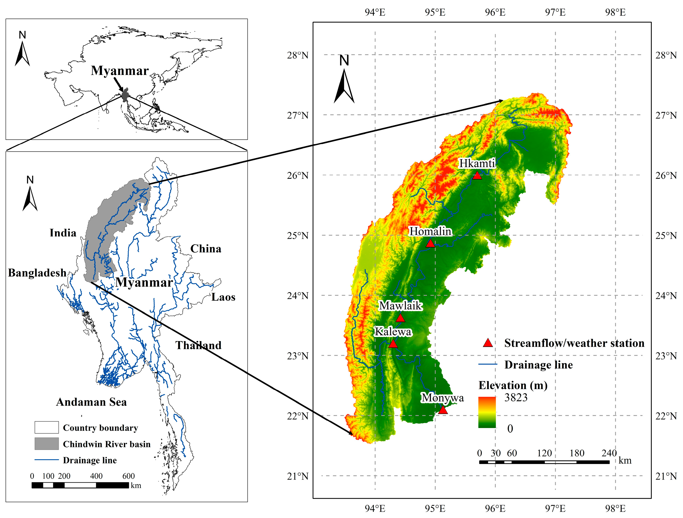
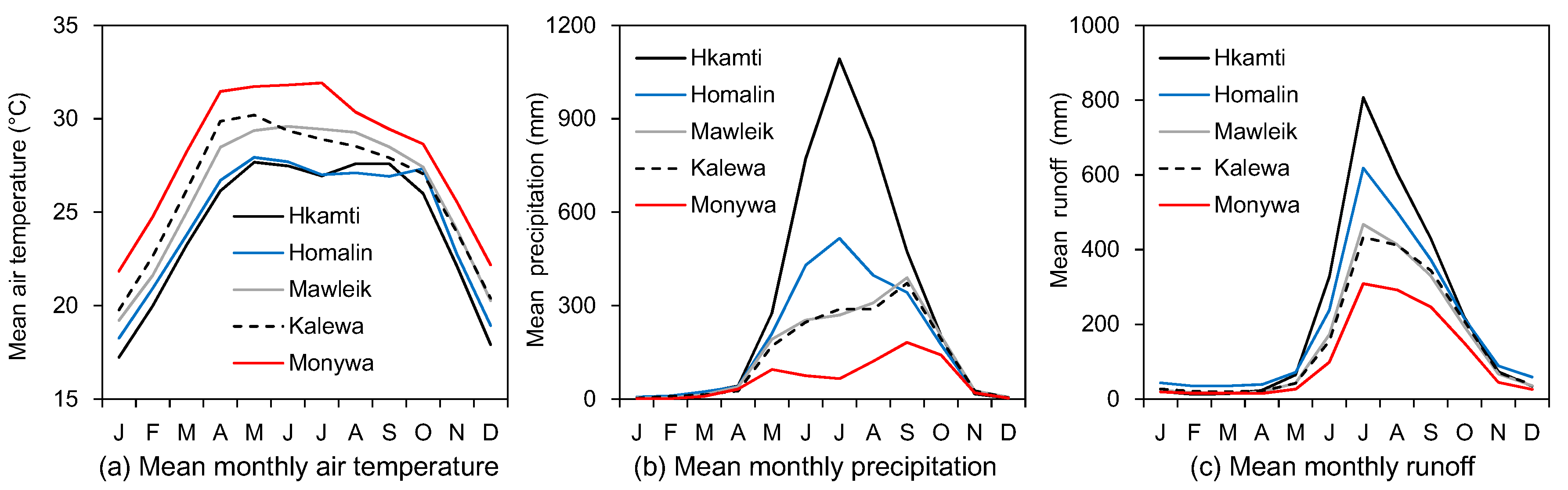
2.1. Study Area

Myanmar is the second largest country in Southeast Asia, sharing borders with China, Laos and Thailand in the east, and Bangladesh and India in the north. It has a 2832 km seaboard with the Indian Ocean to the west and south (Figure 1). There are four main rivers in Myanmar: Ayeyarwaddy, Chindwin, Thanlwin and Sittoung. Among them, the Chindwin River is the third largest river in Myanmar and serves as one of the principal water resources of the country and the most important tributary of Ayeyarwaddy, which is one of the major rivers in Asia. Located in northwestern Myanmar (Figure 1), the Chindwin River basin has a drainage area of 110,350 km2 and a river length of 985 km. It is dominated by a mountainous forested terrain, except for the wide flood plain at its lowest southern part. The river flows into the Central Valley Region, which is the most economically developed area of the country. Several major biodiversity and conservation areas are located in the basin, such as the Hukaung Valley and the Htamanthi wildlife sanctuaries, as well as the Upper Chindwin Catchment Corridor and the Lower Chindwin Forest Corridor with important populations of critically endangered animals [42]. In general, the Chindwin River basin is economically and ecologically important for the development of the country [42].
The Chindwin River basin has subtropical and tropical climates, with distinct humid and dry seasons. The southwest monsoon season starts from June and lasts until September, with a cloudy, rainy, hot, and humid summer. Meanwhile, the northeast monsoon season starts from December and ends in April, with fewer clouds, minimal rainfall, low humidity, and moderate temperature (Figure 2). Precipitation is generally uneven in space due to the effects of the southwest monsoon and the complex topography. According to the precipitation data statistics from five weather stations in the basin (Table 1), the mean annual precipitation exceeds 3700 mm in the northern mountainous source area (Hkamti station) but sharply drops to 750 mm in the southern part (Monywa station). The basin has an annual runoff of 1260–2630 mm, and its spatiotemporal pattern of runoff is similar to that of precipitation (Figure 2). The most dominant land is closed forest (occupying 50% of the basin), followed by degraded forest and shrubs (covering approximately 33%) and agricultural land (covering 15% of the basin area). Shifting cultivation and swamp account for 2%. During the southwest monsoon season, the Chindwin River basin is prone to severe floods every year at one place or another, due to the high rainfall intensities with significant spatial and temporal variations [42,43,44,45]. According to the Department of Meteorology and Hydrology (DMH), Myanmar, flood occurs most frequently in July and August, accounting for 72% of the total number of floods in the basin [42]. The downstream area of the basin is located in the central dry zone of Myanmar, which is the country’s major agricultural region. Owing to less rainfall and higher air temperature, the downstream region is facing frequent droughts, and severe and extreme droughts hit the region in 1997–1998, 2001, 2005, 2008–2009, and 2012–2014 [46]. Severe flood and drought disasters threaten property, human lives, food security and ecological biodiversity in the basin, making it important and urgent to assess flood/drought risks and adopt effective control measures. For flood/drought risk assessment, one fundamental job is to estimate streamflow regimes at any watershed locations through rainfall–runoff modeling. However, the rainfall-monitoring network in the Chindwin River basin is very sparse with a limited number of rain gauges, which likely affects the accuracy of streamflow simulation and forecasting. It is desirable to adopt the satellite precipitation products at fine spatiotemporal resolutions such as IMERG and 3B42V7 as supplementary precipitation data sources for effective runoff simulations. This requires validation of the IMERG and 3B42V7 precipitation estimates and assessment of the feasibility of these two precipitation products in rainfall–runoff modeling.

2.2. Gauge-Based Weather Data

Even though flood and drought hazards prevail in the basin, the local flood/drought management system remains unsatisfactory, particularly for precipitation observations [43]. As shown in Figure 1 and Table 1, merely five weather stations are sparsely distributed in such an extensive basin with a controlled area of 110,350 km2. The daily precipitation data at these five stations from 1 April 2014 to 31 December 2015 were collected from DMH. The daily maximum and minimum air temperature data at these stations for the same period were also obtained. These weather stations collect daily data from 03:00 UTC (Coordinated Universal Time) of the current day to 03:00 UTC of the next day, and the daily precipitation and air temperature data at all the stations are complete from 1 April 2014 to 31 December 2015, with no data missing. These five weather stations are not included in the Global Precipitation Climatology Centre (GPCC) gridded gauge-analysis precipitation data set.
To perform streamflow simulations using a distributed hydrological model, nearest neighbor method was used to interpolate the gauge-based precipitation and air temperature data to the 0.25° spatial scale. The topographical effects were disregarded in the precipitation interpolation, whereas the near-surface air temperature was assumed to decrease by 0.65 °C per altitude rise of 100 m.

2.3. Satellite Precipitation Products

Two types of satellite precipitation products, namely, the TMPA 3B42V7 three-hourly and IMERG final run half-hourly precipitation products, were adopted in this study.
The TMPA 3B42V7 precipitation products were produced by the TRMM TMPA Version 7 algorithm [5]. TMPA can produce microwave-infrared satellite precipitation estimates combined with gauge adjustments and has the potential to give the best precipitation estimates for the regions between 50°S and 50°N on a 0.25° spatial resolution and a three-hour time interval. In this study, the TRMM 3B42V7 three-hourly precipitation product from 1 April 2014 to 31 December 2015 was obtained from the Precipitation Measurement Mission (PMM) website [25], and the three-hourly precipitation data were accumulated to daily values in the study area. The 3B42V7 three-hourly precipitation files are centered on the hour in the file name. For example, a “03z”-hour file represents data from 1:30 UTC to 4:30 UTC. To produce the 3B43V7 daily precipitation data in accord with the time span of daily precipitation collection at the local weather stations (03:00–03:00 UTC), we assigned a half weight (0.5) to the “03z” files for the current and next days, and defined a full weight (1.0) for the “06z”, “09z”, “12z”, “15z”, “18z” and “21z” files for the current day and the “00z” files for the next day.
IMERG is the Level 3 precipitation estimation algorithm of GPM and is intended to inter-calibrate, merge, and interpolate multiple satellite microwave precipitation estimates, microwave-calibrated infrared satellite estimates, precipitation gauge analyses, and other precipitation estimators on a finer spatial resolution (0.1°) with larger quasi-global coverages (60°S–60°N) and a shorter temporal interval (30 min) than those of TMPA products. In this study, the IMERG final run half-hourly precipitation product from 1 April 2014 to 31 December 2015 was downloaded from the PMM website [26], and the IMERG daily precipitation data were produced by simple addition of the 48 half-hourly files covering the time span of 03:00–03:00 UTC.
Both 3B42V7 and IMERG final run products were already bias-corrected on a monthly basis using the GPCC precipitation data set. As stated in Section 2.2, no rain gauges in the basin are included in the GPCC gridded gauge-analysis products. This implies that the GPCC data set covering the study area might not be accurate enough. Therefore, it is necessary to evaluate the quality of these two satellite products using the ground observations, and remove their biases to better suit streamflow modeling. The procedures for quality evaluation and bias-correction of 3B42V7 and IMERG products are described in detail in Section 3.1 and Section 3.2.
To perform hydrological simulations on a spatial resolution of 0.25° (detailed discussion in Section 3.4), the IMERG daily precipitation product was aggregated from a 0.1° spatial resolution to 0.25°. Given that four IMERG grid cells are completely located within a 0.25° grid cell, four fall halfway inside, and a ninth falls one-fourth within, we assigned areal weights of 0.16, 0.08 and 0.04 for these IMERG grid cells, respectively, for precipitation aggregation.

2.4. Streamflow Data

As shown in Figure 1 and Table 1, five streamflow stations are situated in the basin. The daily streamflow data at these five stations from 1995 to 2015 were obtained from the DMH. These stations measure daily streamflow data from 03:00 UTC of the current day to 03:00 UTC of the next day. These historical streamflow data were adopted for the calibration of hydrological models.

3. Methodology

3.1. Evaluation Indicators for Satellite Precipitation Products

The observed historical precipitation records at the five weather stations (Figure 1) in the Chindwin River basin were analyzed to evaluate the accuracy of IMERG and 3B42V7 products. The IMERG and 3B42V7 precipitation estimates at the grid boxes where the weather stations are located were compared with the corresponding gauge-based precipitation from 1 April 2014 to 31 December 2015 at multiple temporal scales.
To comprehensively evaluate IMERG and 3B42V7 precipitation products, six statistical indices were adopted as follows. The Pearson correlation coefficient (CC) describes the agreement between satellite precipitation estimates and gauge observations (Equation (1)). A perfect positive fit is reflected by a CC value of 1, whereas a weak linear correlation is indicated by CC that is close to zero. The relative bias (BIAS) represents the systematic bias of satellite-based precipitation (Equation (2)). A positive BIAS indicates an overestimation of satellite precipitation, whereas a negative value implies an underestimation. The root mean square error (RMSE) measures the average absolute error of satellite precipitation (Equation (3)). The smaller RMSE is, the closer the satellite precipitation estimates are to the observations. CC, BIAS, and RMSE are expressed by
C C = i = 1 n ( P i o P ¯ o ) ( P i s P ¯ s ) i = 1 n ( P i o P ¯ o ) 2 i = 1 n ( P i s P ¯ s ) 2
B I A S = i = 1 n ( P i s P i o ) i = 1 n P i o × 100 %
R M S E = i = 1 n ( P i s P i o ) 2 n
where n is the sample size of the satellite or the gauge-based precipitation time series; P i s and P i o represent the satellite precipitation and gauge-based precipitation amounts at the ith time step (mm); and P ¯ s and P ¯ o are the mean values of satellite precipitation and gauge-based precipitation (mm). The probability of detection (POD), the false alarm ratio (FAR), and the critical success index (CSI) represent the contingency of satellite precipitation estimates. POD, which is also known as the hit rate, describes the fraction of precipitation events correctly detected by the satellite among all real precipitation events (Equation (4)). FAR denotes the fraction of false events among all the events detected by the satellite (Equation (5)). CSI represents the overall fraction of precipitation events correctly detected by the satellite (Equation (6)). POD, FAR, and CSI are expressed by
P O D = H H + M × 100 %
F A R = F H + F × 100 %
C S I = H H + M + F × 100 %
where H denotes the number of real rain events correctly detected by the satellite; M represents the number of real rain events failed to be detected by the satellite; and F is the number of rain events detected by the satellite that do not occur actually. The perfect scores of POD, FAR, and CSI are 1, 0, and 1, respectively.

3.2. Bias-Correction for Satellite Precipitation Products

Several previous studies [31,32,33,34,35,36,37] found that, although 3B42V7 and IMERG products effectively capture the spatiotemporal variations of precipitation in different regions around the world, these estimates still contain considerable errors when compared with ground observations. Given that precipitation inputs are among the most dominant uncertainty sources for hydrological models, satellite precipitation products must be bias-corrected when adopted as the input of a hydrological model for streamflow simulations. In this study, a simple bias-correction scheme was employed to remove the biases of satellite precipitation products. This scheme assumes that the bias characteristics of satellite precipitation at a specified grid box are the same as those at its nearest grid box where a rain gauge is situated. It supposes that if the satellite precipitation at the grid box with a rain gauge is over- or underestimated by a certain percentage, the satellite precipitation estimates at the nearby grid boxes contain the same percentage of biases, and these assumed biases can be removed from the original satellite estimates. The corrected satellite daily precipitation can be expressed as
P d , m s ( x , y ) = P d , m s ( x , y ) × r
r = P m o ( i ) P m s ( x i , y i )
where P d , m s ( x , y ) and P d , m s ( x , y ) denote the original and bias-corrected satellite precipitation amounts on the dth day of the mth month at the grid box [x, y] with the central longitude x and latitude y (mm); r is the bias correction factor; P m o ( i ) is the observed accumulated precipitation amount in the mth month at the ith rain gauge which is the nearest rain gauge to the grid box [x, y] (mm); and P m s ( x i , y i ) is the accumulated original satellite precipitation amount in the mth month at the grid box [xi, yi] where the ith rain gauge is located. This bias-correction scheme could be problematic as it ignores the topographical and meteorological effects on the bias features. However, the number of rain gauges is too limited in this study (five gauges). Thus, deriving the rational relationship between precipitation biases and topographical and meteorological factors for bias correction is difficult. Moreover, the bias correction factor r (Equation (8)) is calculated on a monthly basis rather than at daily time intervals. If r is calculated daily, its value tends to become very large when the gauge-based daily precipitation is very high and the corresponding satellite estimate is very low. This phenomenon is the likely reason why the bias-corrected satellite precipitation at nearby grid boxes is irrationally high.

3.3. Xinanjiang Hydrological Model

The Xinanjiang (XAJ) hydrological model is a lumped, conceptual rainfall–runoff model [47] that is widely applied in humid and semi-humid river basins in China, Vietnam, Japan, and other Asian countries for flood forecasting, water resources evaluation, and accounting design for water quality. In this study the modified version of the XAJ model, namely, the grid-based XAJ model [48], was employed for streamflow simulations, which is a spatially-distributed conceptual hydrological model. This model uses the parameterization scheme of saturation excess runoff to calculate the runoff in each grid cell. In the permeable regions of a grid cell, runoff is produced under the condition that the soil tension water storage reaches its maximum capacity. When precipitation exceeds an open-water evaporation rate, direct runoff is generated at the impervious part. A three-soil-layer module is used to calculate evapotranspiration (ET). The module assumes that ET occurs at the potential ET (PE) rate in the upper layer. Upon exhaustion of the soil tension water in the upper layer, ET continues in the lower layer at a decreased rate that is proportional to the tension water content in that layer. When the total ET in the upper two layers is less than a preset threshold (represented as a fraction of PE), the soil water in the deep layer is exhausted to maintain this preset minimum value. The air temperature-based Hargreaves method [49] is used to calculate the daily PE in XAJ. For runoff concentration and streamflow routing, the XAJ model uses: (1) a gravitational water reservoir to separate the total runoff into three components, namely, surface runoff, interflow runoff, and groundwater runoff; (2) three linear reservoirs to represent runoff concentration for the outflow of each grid cell; and (3) the Muskingum routing method to parameterize the routing effect of the channel system connecting each grid cell.

3.4. Streamflow Simulation Schemes

In this study, the entire Chindwin River basin was separated into 204 grid cells on a 0.25° resolution. Meanwhile, five precipitation data sets were constructed, and they are the gauge-based gridded precipitation data, the original and corrected 3B42V7, and the original and corrected IMERG data sets on a 0.25° resolution. These data sets were used to drive the XAJ model to perform historical daily hydrological simulations at each grid cell in the Chindwin River basin from 1 April 2014 to 31 December 2015, for a total of five simulation runs. For each simulation run, the XAJ model parameters were independently calibrated by fitting the calculated historical daily streamflow time series against the observed data at the five streamflow stations (Figure 1). The calibration period was 1 April 2014–31 December 2014, and the validation period was 1 January 2015–31 December 2015. Model calibration was achieved with the aid of the Shuffled Complex Evolution (SCE-UA) automatic optimization method [50,51]. To derive the model parameters that can comprehensively characterize both high- and low-flow processes, model calibration was performed using the objective function given by
f = m a x ( N S E ) + m a x ( L o g N S E )
N S E = 1 i = 1 n ( Q i s Q i o ) 2 i = 1 n ( Q i o Q o ¯ ) 2
L o g N S E = 1 i = 1 n [ l o g ( Q i s ) l o g ( Q i o ) ] 2 i = 1 n [ l o g ( Q i o ) l o g ( Q o ) ¯ ] 2
where n is the sample size of the observed or calculated streamflow time series; Q i o and Q i s denote the observed and calculated daily streamflow at the ith time step (m3/s); and Q o ¯ and l o g ( Q o ) ¯ represent the mean observed streamflow and mean log-transformed observed streamflow (m3/s), respectively. The five sets of simulated streamflow time series using different precipitation inputs were compared against the observed streamflow to assess the feasibility of 3B42V7 and IMERG precipitation products in streamflow simulations in the study area. The accuracy of streamflow simulations were evaluated using four statistical indices, namely, BIAS, CC, NSE, and LogNSE. Detailed description of streamflow simulation schemes can be found in Supplementary Material S1.

4. Results

4.1. Evaluation of Satellite Precipitation Products

The 3B42V7 and IMERG precipitation products covering the entire Chindwin River basin from 1 April 2014 to 31 December 2015 were evaluated in terms of spatial patterns and errors in daily and monthly precipitation.

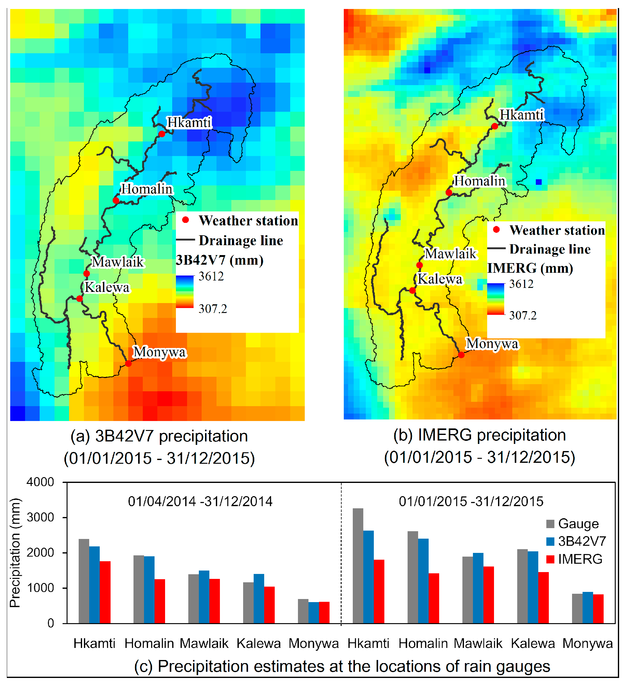
4.1.1. Spatial Patterns

Figure 3a,b shows the spatial patterns of 3B42V7 and IMERG precipitation estimates from 1 January to 31 December 2015 in the Chindwin River basin. Both products represented a similar spatial pattern: precipitation tended to decrease from north to south. The amount of maximum annual precipitation in 2015 appeared in the source region of the basin, reaching 3345.6 mm for IMERG and 3167.6 mm for 3B42V7. The lowest amount generally occurred in the grid cells near the watershed outlet, reaching 715.2 mm for IMERG and 892.3 mm for 3B42V7. Figure 3c illustrates that the observed precipitation is in a remarkable decreasing trend from the upper to the lower reach for both periods (1 April–31 December 2014 and 1 January–31 December 2015). Both IMERG and 3B42V7 manifested a similar trend but generally underestimated the precipitation in most grid boxes where the rain gauges are located, particularly at the upstream gauges. For instance, IMERG and 3B42V7 underestimated the precipitation at the Hkamti station by 44.7% and 19.4% from 1 January to 31 December 2015. Given that IMERG estimates precipitation on a much finer resolution than 3B42V7, the former can provide more detailed spatial features of precipitation than the latter (Figure 3a,b). Overall, 3B42V7 provided considerably higher precipitation estimates than IMERG. From 1 January to 31 December 2015, 3B42V7 estimated the amount of basin-averaged precipitation to be 2014.0 mm, whereas IMERG provided an estimation of 1720.1 mm, which is 14.6% less than that of the 3B42V7 product.

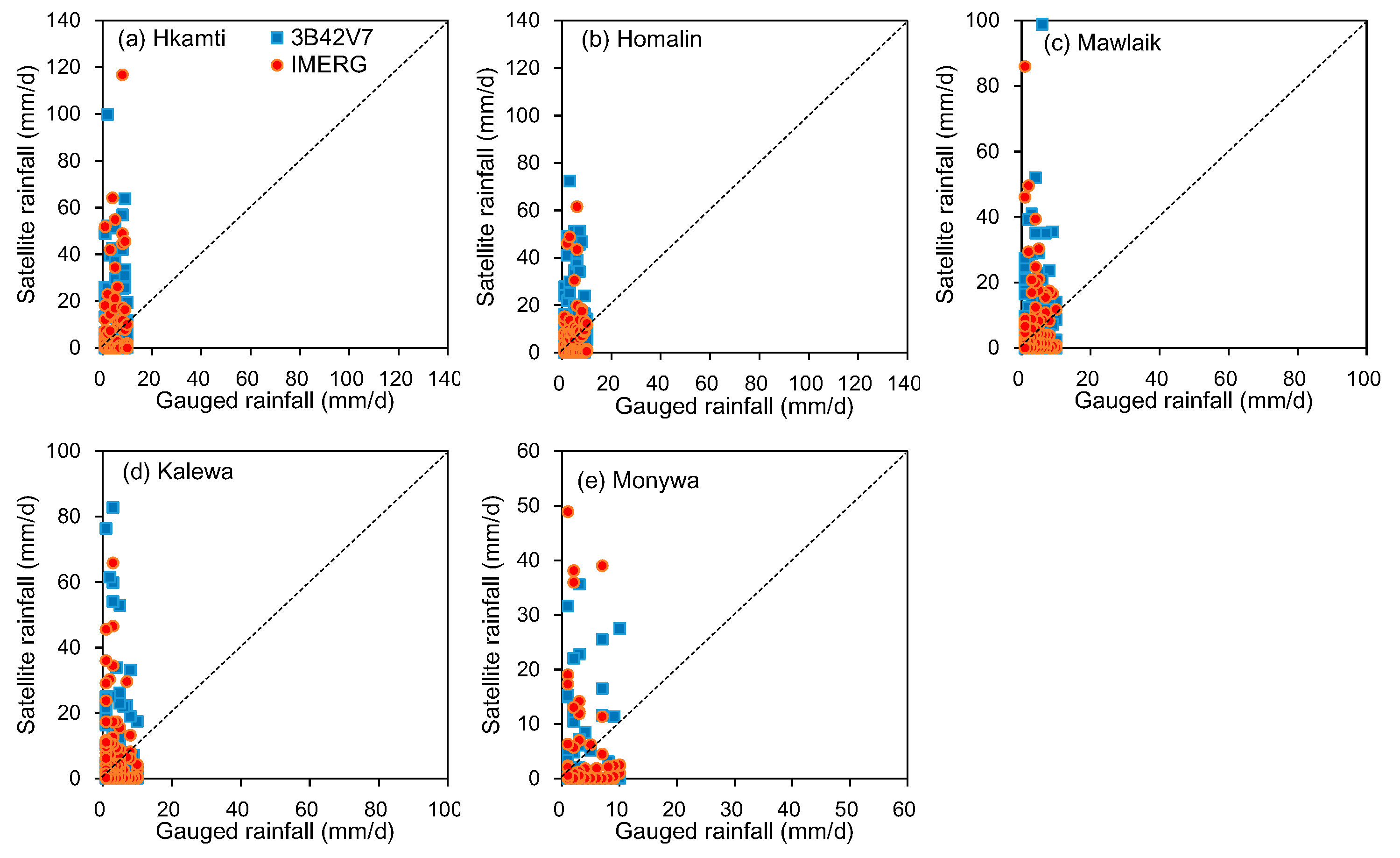
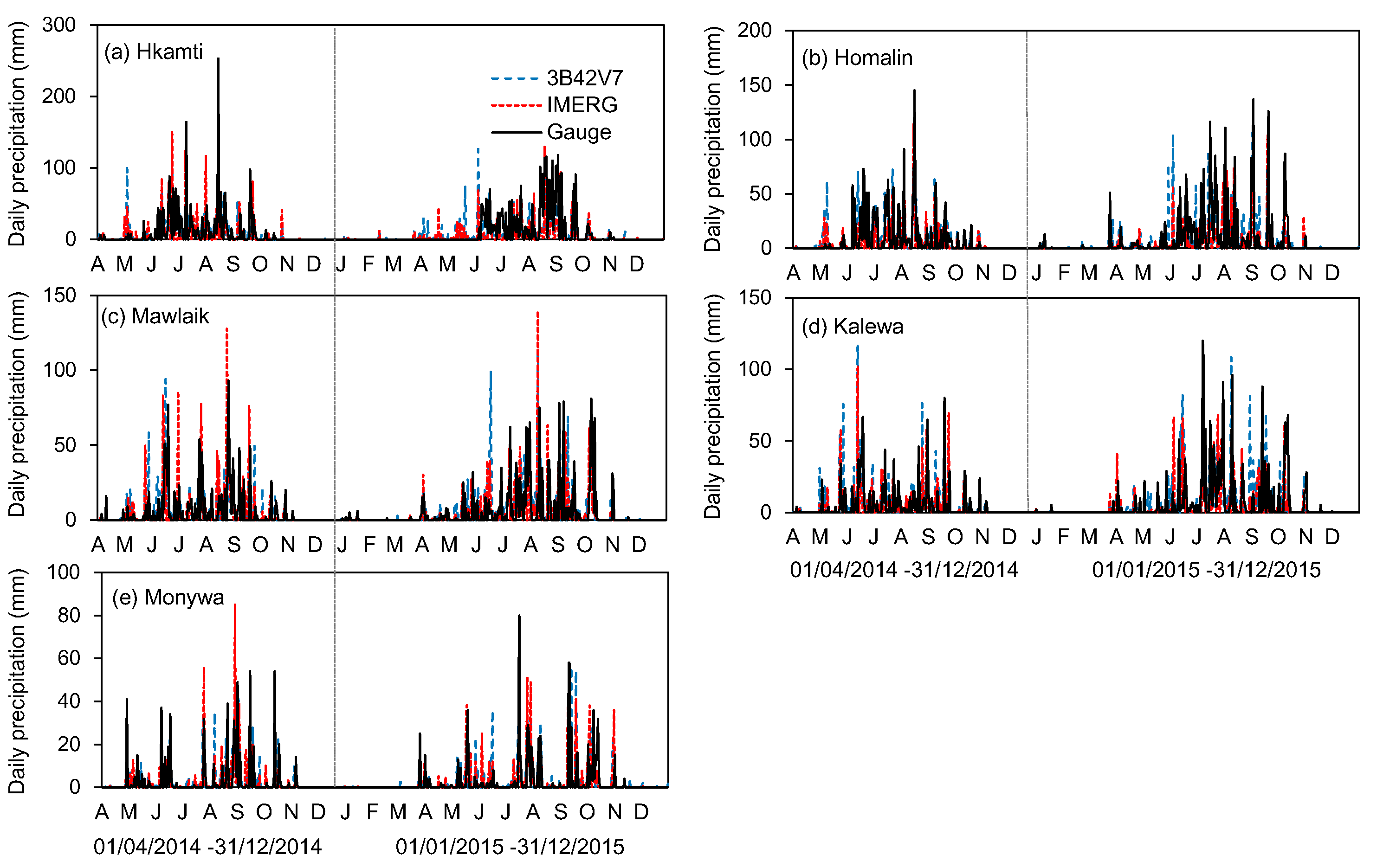
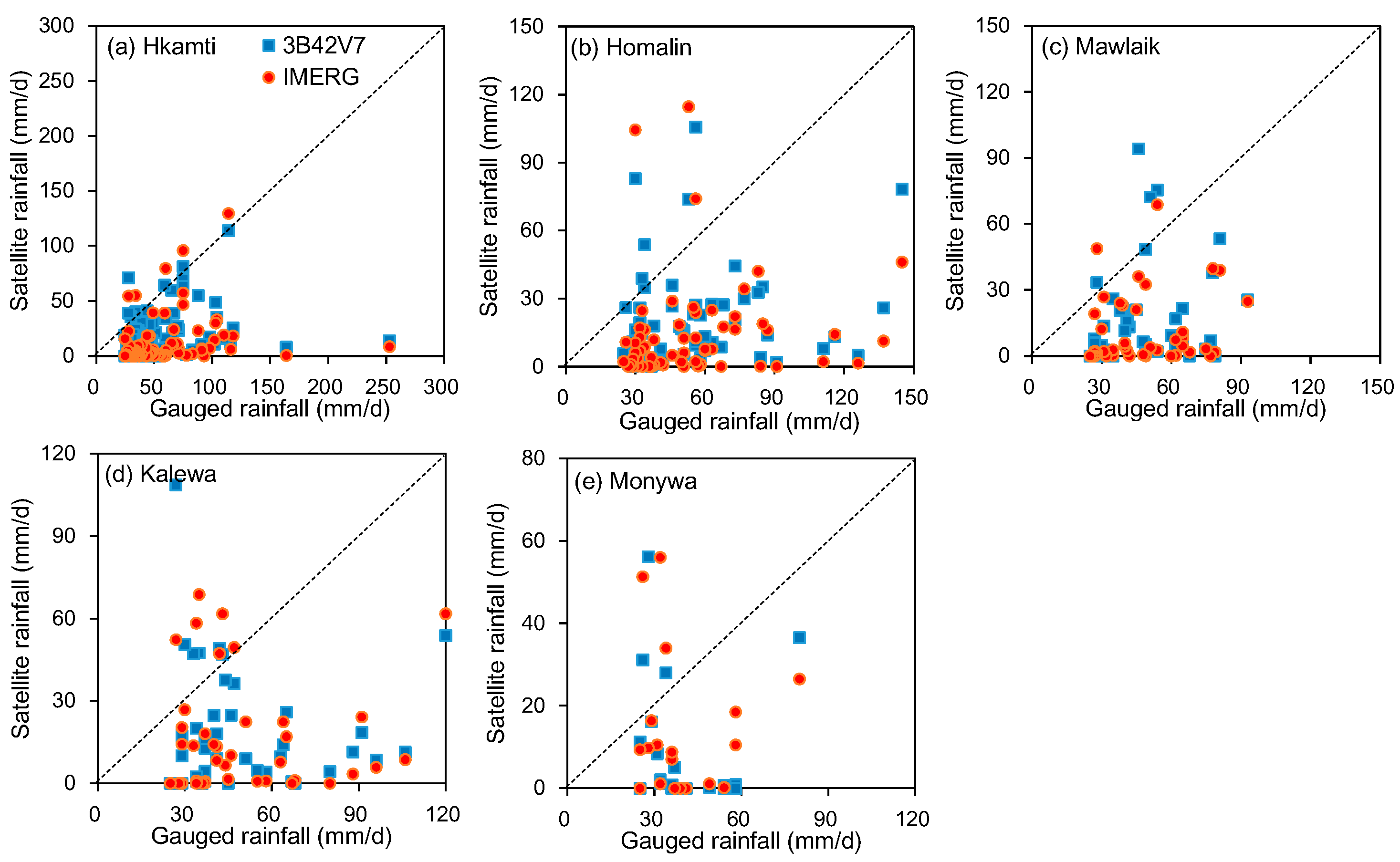
4.1.2. Daily Precipitation

To evaluate the quality of 3B42V7 and IMERG products, the daily precipitation estimates of these two satellite products at the locations of the five rain gauges were derived and compared with the gauge-based precipitation. Figure 4 shows that both 3B42V7 and IMERG can capture the temporal variation patterns of daily precipitation at the five rain gauges. However, Table 2 indicates that these two products still contain considerable errors. The values of CC for both products were considerably low, ranging from 0.247 to 0.356 between the 3B42V7 estimates and the observations, and from 0.224 to 0.316 between the IMERG estimates and the gauge-based precipitation. 3B42V7 had a much higher CC than IMERG at the Hkamti, Homalin and Mawlaik stations, and IMERG had a slightly higher CC than 3B42V7 at the Kalewa and Monywa stations. IMERG underestimated precipitation at all the five rain gages, particularly at the Hkamti and Homalin stations, displaying a large negative BIAS of −37.1% and −41.2%. 3B42V7 presented significant underestimation at Hkamti (14.9% BIAS), a slight underestimation of daily precipitation at Homalin and Monywa (by 5.2% and 2.7%), and a moderate overestimation at Mawlaik and Kalewa (BIAS of 6.4% and 5.4%). In terms of RMSE, both products contained similar magnitudes of errors. Regarding the contingency of satellite precipitation estimates, the POD values were low at all the rain gauges, ranging from 0.092 to 0.299 for 3B42V7 and from 0.117 to 0.207 for IMERG, implying that 3B42V7 and IMERG correctly identified real rainfall events by 29.9% and 20.7% at most. Moreover, Table 2 indicates that both products had comparatively large FAR and small CSI values, implying considerable errors in the two satellite products. Comparison of all statistical indices in Table 2 reveals that 3B42V7 is more accurate than IMERG at the Hkamti, Homalin, Mawlaik, and Kalewa stations but is slightly less accurate at the Monywa station.
To assess the performance of IMERG and 3B42V7 products in detecting historical heavy precipitation events, we defined the gauge-based daily precipitation exceeding 25 mm as a real heavy precipitation event. The observed daily precipitation during heavy precipitation events was compared with the corresponding satellite estimates (Figure 5). Table 3 shows that both IMERG and 3B42V7 were poorly correlated with the gauge-measured heavy precipitation, having CC values of less than 0.270. As shown in Figure 5 and Table 3, these two satellite products largely underestimated precipitation during heavy rain events by over 62%. 3B42V7 presented a slightly smaller magnitude of underestimation than IMERG, except at the Monywa station. RMSE for both products generally exceeded 35 mm. According to the POD statistics in Table 3, 3B42V7 captured 20.0%–31.7% of real heavy rain events, whereas IMERG captured 13.3%–20.0%. In general, both products displayed poor performance in heavy rain identifications and estimations. 3B42V7 had a slightly higher accuracy than IMERG, except at the Monywa station.
To analyze the accuracy of satellite products in light rain estimations, we defined the observed daily precipitation ranging from 0.1 mm to 10.0 mm as a real light rain event. The gauge-based daily precipitation during light rain events was compared with the corresponding satellite estimates (Figure 6). Similar to the situation for heavy rain estimations, both products were poorly correlated with gauge-based light rain events (Table 3). IMERG and 3B42V7 significantly overestimated precipitation during light rain events by 22.4%–65.8% and 27.8%–116.1% (Figure 6 and Table 3). Nonetheless, more than 30% of actual light rain events were effectively detected by IMERG and 3B42V7. Overall, both products manifested similar low accuracies for light rain estimations at all the gauges.

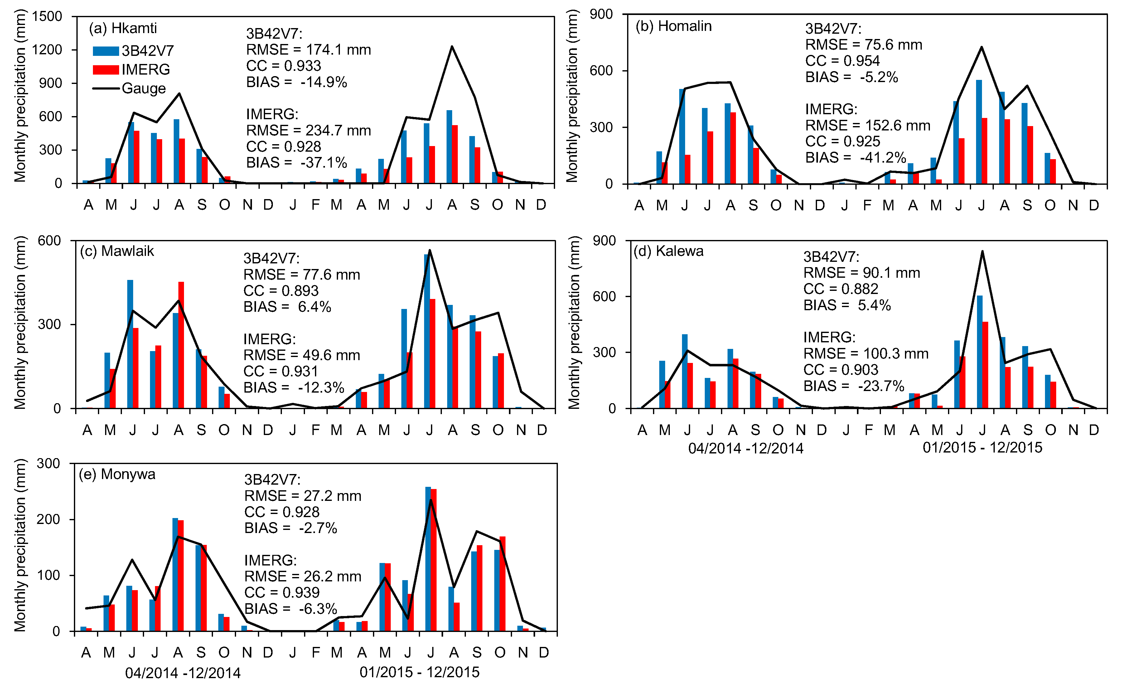
4.1.3. Monthly Precipitation

The daily precipitation estimates from IMERG and 3B42V7 at the five gauges were aggregated to monthly time series, and they were compared with the observed monthly precipitation. As shown in Figure 7, both IMERG and 3B42V7 products generally followed the variation patterns of monthly precipitation that were similar to those recorded by the rain gauges. Although the aggregation of the satellite precipitation estimates from a daily scale to a monthly scale cannot change the magnitudes of their systematic errors (BIAS), the linear correlations between the satellite precipitation and the observations were significantly improved (Figure 7). The CC values were increased in the range of 0.882–0.954 for 3B42V7 and 0.903–0.939 for IMERG. The possible reason for this improvement is that although both IMERG and 3B42V7 were comparatively inaccurate to characterize daily precipitation variability, they generally captured precipitation seasonality in the Chindwin River basin, which is indicated in Figure 4. Overall, 3B42V7 performed better than IMERG in estimating monthly precipitation at the Hkamti, Homalin, and Kalewa stations, whereas IMERG had higher accuracy than 3B42V7 at the Mawlaik and Monywa stations.

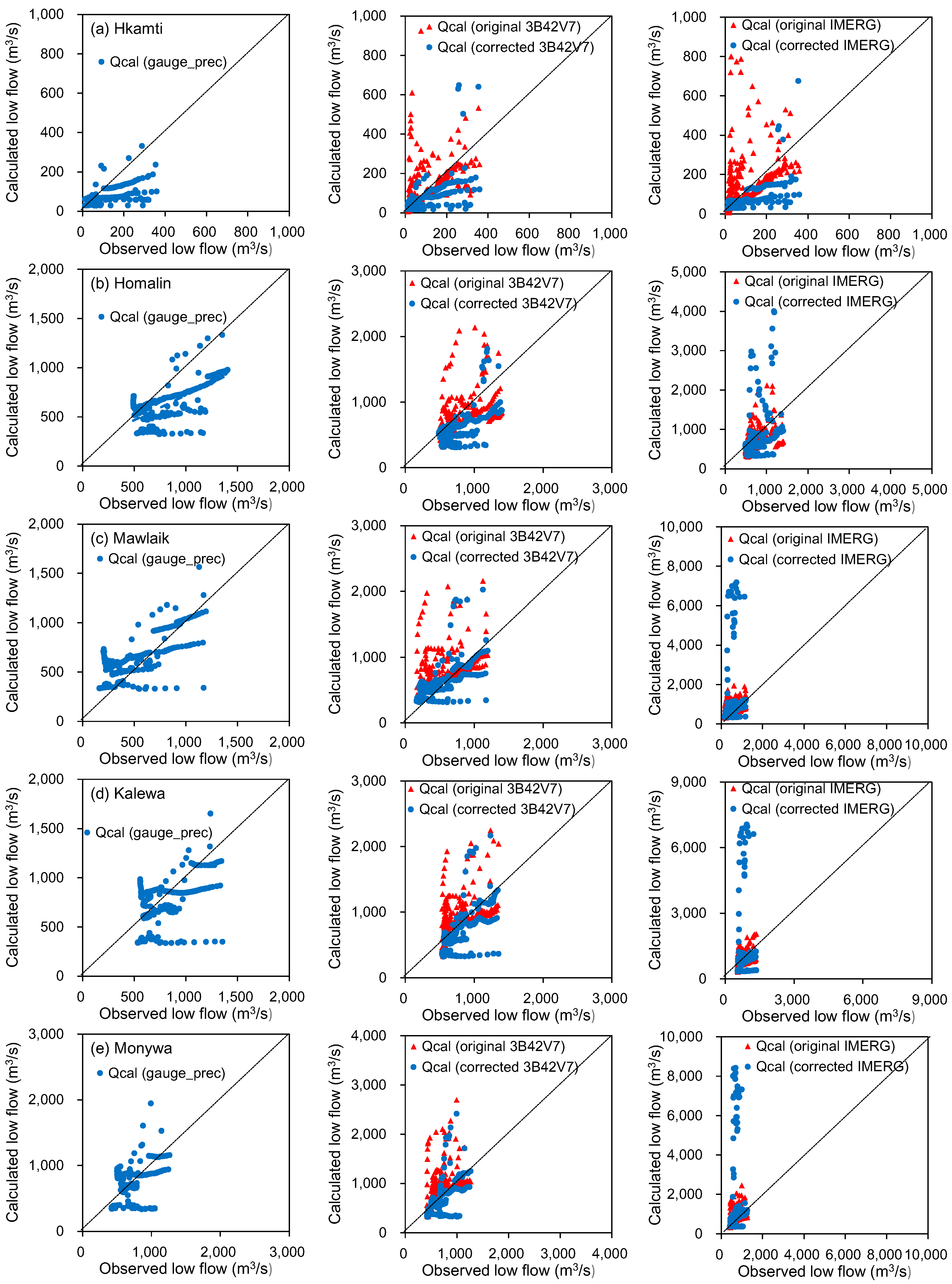
4.2. Evaluation of Streamflow Simulations

As mentioned in Section 4.1, both IMERG and 3B42V7 products contained non-negligible errors. Their biases must be removed before they can be employed for streamflow simulations to effectively reduce the uncertainties of hydrological models arising from precipitation inputs. By applying the bias-correction method described in Section 3.2, both IMERG and 3B42V7 daily precipitation products on a 0.25° resolution were corrected over the entire basin. Consequently, five precipitation data sets were constructed, namely, the gauge-based precipitation data, the original and corrected 3B42V7 data sets, and the original and corrected IMERG data sets. Subsequently, the XAJ model was driven by these five data sets to perform daily streamflow simulations from 1 April 2014 to 31 December 2015. The simulated streamflow processes using the five different precipitation inputs were compared with the observed streamflow to evaluate the feasibility of satellite precipitation products in streamflow simulations.

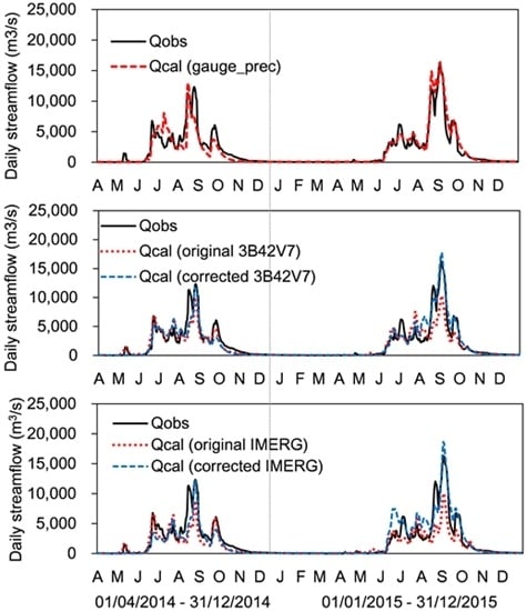
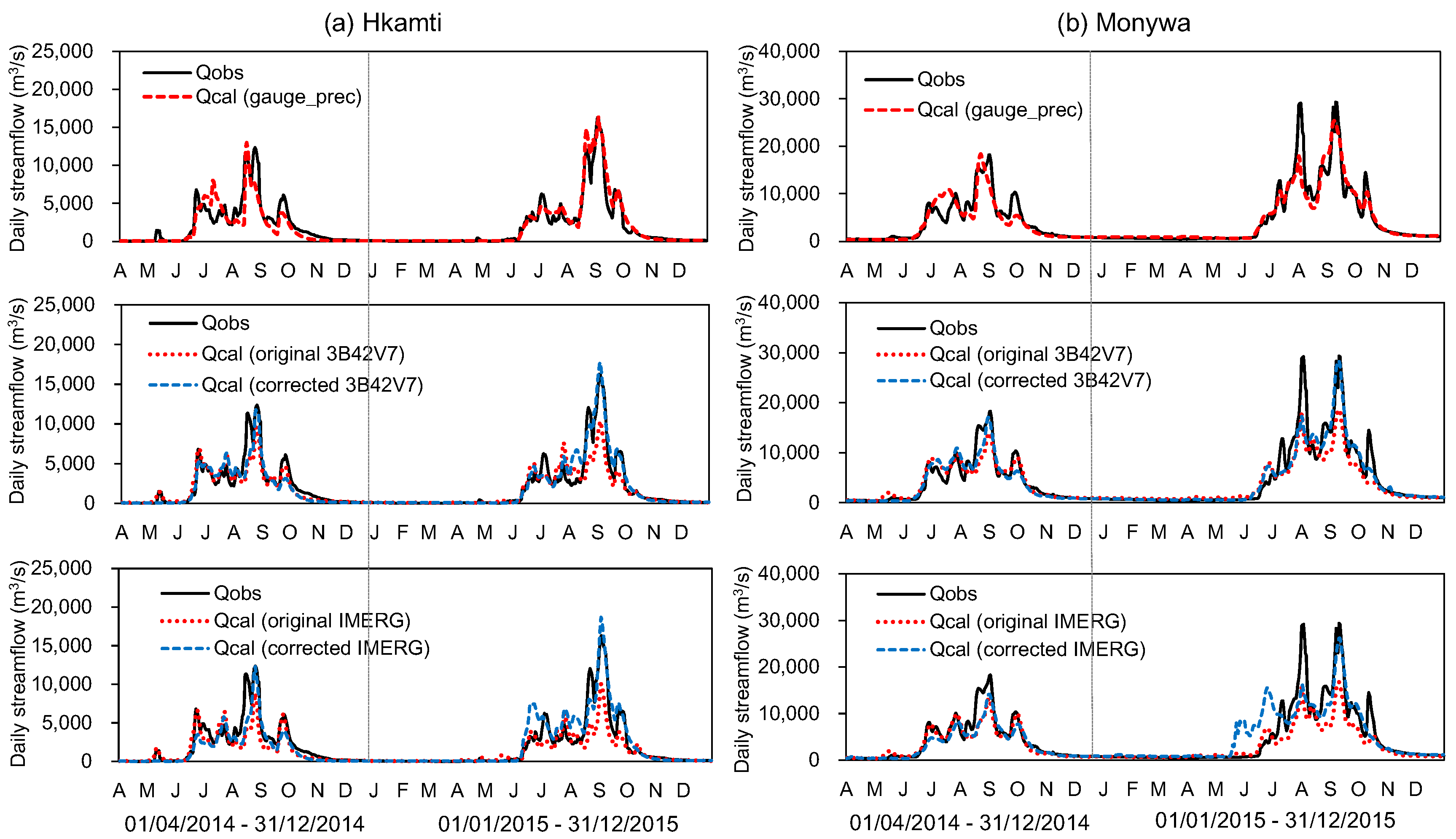
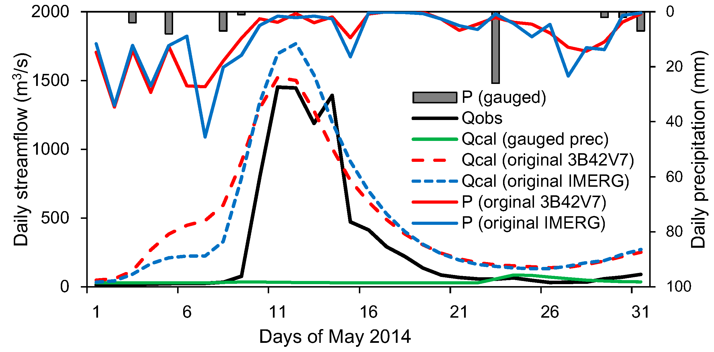
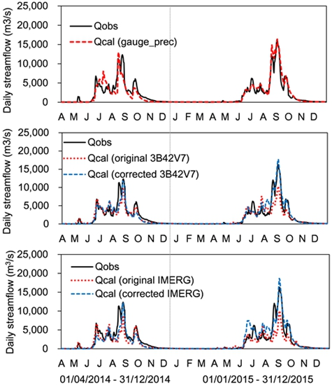
4.2.1. Daily Streamflow

Figure 8 depicts the daily hydrographs at the Hkamti and Monywa stations that were simulated using different precipitation inputs. All five simulation runs captured the temporal variation patterns of streamflow that were similar to the observed discharge. Frequent high flows occurred from June to September, whereas low flows were mainly observed from December to April. Figure 8 and Table 4 show that although rain gauges are sparsely distributed in the Chindwin River basin (merely five gauges in a controlled area of 110,350 km2), the XAJ model, driven by the gridded precipitation data set that was interpolated from the five rain gauges, satisfactorily reproduced the daily streamflow processes at all five stations from 1 April 2014 to 31 December 2015. This simulation run slightly underestimated the daily streamflow by 0.7%–5.2%, with NSE and LogNSE exceeding 0.82 and 0.85. These findings indicate the sound performance of the XAJ model in simulating both high- and low-flow processes.
Given that both IMERG and 3B42V7 products contained considerable errors in precipitation estimates, the two modeling runs that utilized the gridded precipitation data sets derived from the original IMERG and 3B42V7 products produced generally poorer simulations than the gauge-based simulations in terms of all statistical indices in Table 4. Moreover, because IMERG underestimated precipitation at all the rain gauges, particularly gaining a considerably large BIAS in upstream gauges (−37.1% and −41.2% at the Hkamti and Homalin stations, Table 2), the streamflow simulated by the XAJ model with the original IMERG precipitation as its input was approximately 23.5%–31.2% systematically lower than the observed discharge (Table 4). Meanwhile, 3B42V7 presented smaller systematic errors in precipitation at the Homalin, Mawlaik, Kalewa, and Monywa stations (−5.2%–6.4% BIAS); however, 3B42V7 significantly underestimated precipitation at Hkamti, which was the source region station (Table 2). Consequently, the XAJ model systematically underestimated the streamflow at Hkamti by 16.6%, and this systematic bias propagated to the downstream stations, causing the simulated discharge at these stations to be 10.9%–16.9% lower than the measurements. Figure 8 illustrates that a few simulated flood peaks were remarkably lower than the actual ones in the two modeling runs using the original satellite products. This phenomenon mainly resulted from the underestimation of precipitation by both IMERG and 3B42V7 during heavy rain events. Table 4 shows that the simulation run using the original 3B42V7 product was generally better than that using the original IMERG precipitation. Although the satellite precipitation products and gauge-based precipitation data were in a very poor correlation on daily basis (Table 2 and Table 3), the CC values for daily streamflow simulations using the original IMERG and 3B42V7 products were significantly increased (Table 4). The possible reason for this phenomenon is that both IMERG and 3B42V7 are able to effectively capture the seasonal cycle of precipitation in the Chindwin River basin (Figure 7), which facilitates to reproduce rational streamflow processes in both wet and dry seasons. Meanwhile, the observed streamflow time series shows high seasonality, which is generally easy for hydrological models to reproduce. In addition, hydrological models are, to some degree, tolerant to the errors of precipitation inputs, and model parameter calibration is able to partially offset the streamflow biases resulting from inaccurate precipitation inputs. For example, the XAJ model uses the highly sensitive parameter K (the coefficient of PE) to calculate PE, and a larger K tends to produce higher actual ET and thus generate lower total runoff. Table S1 shows that the calibrated parameter K in the area controlled by the Hkamti station decreased from 1.379 in the gauge-based model run to 0.838 in the original IMERG-based simulation. As a result, model recalibration effectively damped the magnitude of runoff reduction that resulted from the significant precipitation underestimation in IMERG. Another example is the sensitive parameter SM (the areal mean free water storage capacity), and a smaller SM usually generates higher flood peaks. As indicated in Table S1, SM in the original IMERG-based run was much lower than that in the gauged-based run. The decreased SM partially compensated for the reduction in high flows arising from the systematical underestimation of heavy rain events in IMERG.
Figure 8 and Table 4 demonstrate that bias correction of satellite precipitation products significantly improved the performance of streamflow simulations. The simulations using the corrected 3B42V7 precipitation achieved an even higher accuracy than those using the gauge-based precipitation, implying that the 3B42V7 product can effectively characterize the spatiotemporal features of precipitation in the study area. It also suggests that the bias-corrected 3B42V7 data set likely improved the hydrological simulations in the studied watershed where rain gauges are sparsely distributed. The XAJ model generally performed better in terms of BIAS and NSE when driven by the corrected IMERG data set than when driven by the original IMERG precipitation input. However, the CC and LogNSE values substantially decreased at the Mawlaik, Kalewa, and Monywa stations. Figure 8b shows that the modeling performance at Monywa even worsened in May–June 2015, overestimating the calculated streamflow presumably because of the large uncertainty of the bias-correction method for satellite precipitation products. As mentioned in Section 3.2, the bias correction of satellite precipitation was conducted under the assumption that the satellite precipitation product at the grid cells near a specified rain gauge has the same magnitude of biases (BIAS) as the precipitation estimates at that rain gauge. In this study, IMERG estimated the total precipitation amount at Homalin and Kalewa in May 2015 to be 9.6 mm and 12.0 mm, whereas the corresponding observations were 84.0 mm and 92.0 mm. According to Equations (7) and (8), the bias correction factor r was calculated to be 8.75 and 7.67 for the grid boxes surrounding Homalin and Kalewa. The original IMERG precipitation estimates at the grid cells near Homalin and Kalewa were amplified by 8.75 and 7.67 times to reach the corresponding corrected precipitation. This procedure of utilizing extremely large bias correction factors produced irrationally high precipitation values at a few grid cells, thereby generating distinct higher basin-averaged precipitation and ultimately leading to discharge overestimation at the basin outlet in May–June 2015.
To further investigate the performance of high- and low-flow simulations using the satellite precipitation inputs, we defined the observed daily streamflow exceeding its 90% quantile as high flow and that less than its 50% quantile as low flow. The observed high- and low-flow data points were compared with the corresponding simulated flow with various precipitation inputs. As shown in Figure 9 and Table 4, the simulations with the gauge-based gridded precipitation input moderately underestimated the high flow at all the stations by 1.8%–11.5%. When the XAJ model was driven by the original 3B42V7 and IMERG products, the percentage of high flow underestimation was worsened to 29.5%–39.3% and 39.1%–48.9%, mainly because of the large negative biases of heavy rain estimates in these two satellite products (Table 3). The bias correction of the satellite products effectively improved the high-flow simulations. In the simulations using the corrected 3B42V7 and IMERG precipitation inputs, the computed high flow was 9.3%–16.6% and 11.5%–25.8% lower than the observations. Table 4 shows that in terms of CC, the high flow simulations using the corrected 3B42V7 precipitation were more accurate than that using the gauge-based precipitation. It also indicates that the performance of the high-flow simulations using the original (corrected) 3B42V7 product was generally better than that using the original (corrected) IMERG precipitation for BIAS and CC statistical indices.
Among the five low-flow simulation runs using the different precipitation inputs, the gauged-based runs generally had the highest accuracy (Figure 10 and Table 4). The bias correction of the 3B42V7 product effectively reduced the low-flow errors at all hydrological stations, and the performance of the corrected 3B42V7-based simulations was slightly worse than the gauge-based runs. However, the bias correction of the IMERG precipitation estimates improved the low-flow simulation at the Hkamti station but not for the other four stations. As discussed above, the corrected IMERG precipitation at Homalin and Kalewa in May 2015 was largely overestimated due to the uncertainty of the bias-correction method. Consequently, the simulated daily discharge was considerably higher than the observations at the Homalin, Mawlaik, Kalewa, and Monywa stations in May–June 2015, during which a few low flows actually occurred (Figure 8b). These errors further diminished the general performance of low-flow simulations at these stations. Overall, the low-flow simulations using the original (corrected) 3B42V7 product generally performed better than those using the original (corrected) IMERG precipitation.

4.2.2. Monthly Streamflow

The calculated daily streamflow time series using the five different precipitation inputs were aggregated to monthly time series, and the performance of the monthly streamflow simulations was evaluated. Table S2 shows that the monthly streamflow simulations were generally more accurate than the daily simulations in terms of CC and NSE, although both simulations had the same magnitudes of BIAS. Figure S1 shows that when the original IMERG and 3B42V7 data sets were used, the simulated monthly streamflow in August 2014 and July–October 2015 was considerably underestimated. However, in simulations using the corrected IMERG and 3B42V7 products, the calculated monthly hydrographs agreed well with the observed data during the entire simulation period, except for May and June 2015 when the corrected IMERG-based model run significantly overestimated the monthly streamflow. In general, the bias-corrected satellite precipitation products were feasible in historical monthly streamflow simulations in the Chindwin River and yielded comparable skill scores as the model run with the gauge-based precipitation data set. Meanwhile, simulations with the corrected 3B42V7 product generated more accurate simulated monthly streamflow than those using the corrected IMERG data set.

5. Discussion

The latest GPM Core Observatory sensors and new calibration algorithms were developed to improve the performance of GPM constellation satellites in observing precipitation at much finer spatiotemporal scales than their predecessor, TRMM. A few recent studies have proven that the GPM IMERG products are generally superior to TRMM in several regions, such as the Xinjiang region [30] and the Qinghai-Tibetan Plateau in China [30,31]; Mainland China [33,34]; Guilan, Bushehr, Kermanshah, and Tehran regions in Iran [37]; Far-East Asia [35]; and India [36]. However, in the present study, although the daily precipitation data of both the IMERG final run and TMPA 3B42V7 captured the spatiotemporal variation patterns of rainfall events in the Chindwin River basin in Myanmar, no significant improvements were found in IMERG. Furthermore, the 3B42V7 data set even outperformed IMERG at the daily and monthly time scales and in heavy rain event detections at four out of the five gauges. These findings strengthen the urgent need to further improve GPM algorithms, particularly for data-sparse regions with complex terrains in Myanmar.
This study demonstrates that the non-negligible errors in the two satellite precipitation products significantly propagated to streamflow simulations. The significant negative biases in total precipitation amount and heavy rain estimates, to a large extent, caused the noticeable underestimation of total runoff and high flow, with IMERG-based simulations demonstrating a considerably worse performance than 3B42V7. Despite the inherent considerable biases, both the original IMERG and 3B42V7 products were, in certain periods, superior to the gauge-based data in hydrologic applications. Figure 11 indicates that the two satellite products estimated the areal mean precipitation in the region controlled by the Hkamti station to be 303.5 mm and 286.3 mm in May 2014. Thus, the corresponding simulated hydrographs agreed well with the observed data. By contrast, only one gauge was situated in the drainage area of Hkamti, and the basin-averaged precipitation derived from gauge data was negatively biased to be 57.0 mm, thus producing a much lower streamflow than the measured values. This result proves that both IMERG and 3B42V7 accurately captured the spatiotemporal features of precipitation in May 2014 and therefore facilitated streamflow simulations. It also highlights the necessity for the local government to build a denser rain gauge network in the basin. In addition, a monthly-based simple bias-correction method was applied to the two satellite data sets and effectively improved the overall performance of streamflow simulations. The corrected 3B42V7-based simulations performed slightly better than that using the gauge-based precipitation, implying that the 3B42V7 product can potentially improve the discharge simulations over the data-sparse Chindwin River. In regions where a sufficiently dense gauge network is unavailable, satellite-derived rainfall can be a critical data source for identifying hazards from small-scale rainfall and flood events [52].
The hydrological utility of satellite precipitation products is associated with large uncertainties from bias-correction methods, parameter estimations, and model structures. In this study, improved streamflow simulations were achieved via bias correction. However, the method adopted in this study sometimes produced irrationally high precipitation values at a few grid cells, resulting in overestimated discharge in certain periods. Therefore, a better bias-correction method should be developed in the future, and the uncertainties introduced by bias-correction procedures should be quantified.
Ideally, the parameters of a hydrological model should be calibrated using the “perfect” observed precipitation data set measured in a dense gauge network. These values of calibrated parameters can be considered as the best possible approximation of watershed hydrological features, and they should be adopted for all simulation runs using different satellite precipitation inputs. Nevertheless, this study recalibrated the XAJ model using the satellite products, instead of using the model parameters, based on the gauge-based gridded data. This is because the gauge-based precipitation data were derived from sparsely distributed rain gauge records and are therefore inadequate for characterizing the actual rainfall regimes for model calibration. A few studies [6,21] found that recalibration can sometimes cause parameter values to exceed their reasonable ranges. To avoid this problem, we defined the searching space of each XAJ model parameter to be strictly within its physical range in the SCE-UA optimization algorithm. Thus, with the recalibrated model parameters, the streamflow simulations fed with the satellite precipitation data are likely to produce more accurate results than the case wherein the “perfect” parameter set is used, given that a few model parameters are flexible and sensitive to changes in precipitation inputs. Such characteristics raise the issue of parameter uncertainties, which significantly influence the evaluation of satellite precipitation products in hydrological simulations. This issue will be investigated thoroughly in the future.
Precipitation resampling and interpolation were conducted in this study to make the different satellite and gauge-based data sets comparable. Although IMERG products are on a finer resolution (0.1°), this study found that 3B42V7 is better suited than IMERG. In this research, IMERG products were aggregated from a 0.1° spatial resolution to 0.25° for comparison with 3B42V7. This procedure may have produced some errors. Moreover, the gauged-based precipitation data were interpolated to 0.25° gridded precipitation data set for hydrological simulations without consideration of topological effects. This is likely to cause some errors and further effect streamflow simulations. In future works, the possible errors introduced by these procedures should be evaluated. In addition, more suitable rainfall–runoff models should be applied in this region, and the simulated streamflow from different models should be compared and analyzed to quantify the inherent uncertainties from model structures.
Despite the poor correlation between the ground precipitation observations and the two satellite products (Table 2), the XAJ model driven by the satellite rainfall estimates was able to reproduce streamflow both in the original and in the corrected versions (Table 4). As discussed above, part of this is due to the model recalibration. Another reason could be also the high seasonality of the flood time series, which is quite easy for hydrological models to reproduce. To fairly evaluate the feasibility of satellite precipitation products in streamflow simulation, the seasonal cycle should be removed from the streamflow time series and the simulated streamflow anomalies should be validated against the observations. The work will be employed in the near future.

6. Conclusions

In this study, GPM and TRMM satellite precipitation products and their feasibility in streamflow simulations was initially evaluated at daily and monthly scales in the data-sparse Chindwin River basin in Myanmar. The main findings of this study are as follows:
(1)
In general, IMERG and 3B42V7 represent a similar spatial pattern over the Chindwin River basin, demonstrating a decreasing trend from north to south. IMERG provides a more detailed spatial information of precipitation than 3B42V7, due to its native resolution of 0.1° × 0.1° compared to 3B42V7’s 0.25° × 0.25°.
(2)
Although IMERG and 3B42V7 can capture the temporal variation patterns of daily precipitation at the five rain gauges, these two products still contain considerable errors. IMERG significantly underestimates the total precipitation at all the gauges, and 3B42V7 presents a moderate underestimation at three out of the five gauges. Both products performed poorly in heavy- and light-rain detections and estimations, with a considerable underestimation of heavy-rain estimates and a significant positive bias of light-rain estimates. The accuracy of IMERG and 3B42V7 in estimating monthly precipitation is significantly improved, compared to daily precipitation estimates. Overall, 3B42V7 outperforms IMERG at four out of the five gauges.
(3)
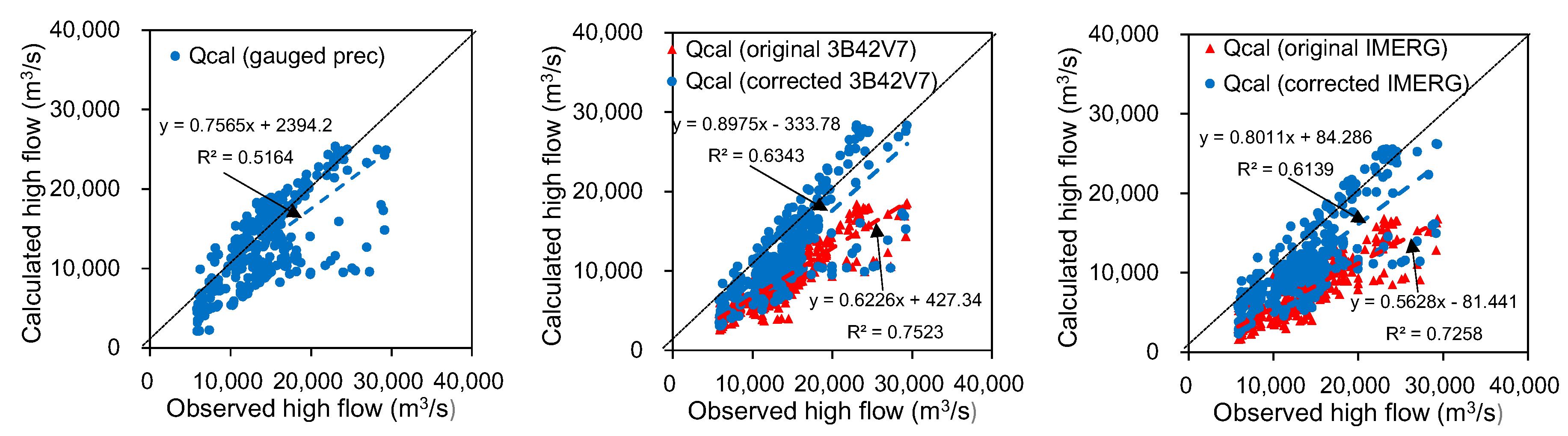
The large errors in IMERG and 3B42V7 distinctly spread in streamflow simulations via the XAJ hydrological model, with the significant systematic underestimation of total runoff and high flow. The IMERG-based simulations perform worse than those of 3B42V7. The bias correction of satellite precipitation estimates effectively improves the performance of daily and monthly streamflow simulations using IMERG and 3B42V7 data sets. The corrected 3B42V7-based simulations perform slightly better than those using the gauge-based precipitation. In general, IMERG and 3B42V7 are both feasible in streamflow simulations in the Chindwin River basin, with the 3B42V7 product being better suited than IMERG.
The above findings provide GPM researchers with timely and useful feedbacks from Myanmar as regards the quality of IMERG products. The newly developed GPM Core sensors and calibration algorithms are not yet able to produce more accurate precipitation estimates than its predecessor, TRMM in the Chindwin River basin. This finding highlights the need for GPM developers to refine the algorithms and improve the accuracy of IMERG products in Myanmar, where plenty of rainfall data are urgently needed for hydrological utilities. Moreover, it emphasizes that local authorities must establish a denser rainfall observation network, which not only facilitates the validation of satellite-derived precipitation but also helps improve the accuracy of streamflow simulations/forecasting for effective flood warning and disaster mitigation.

Supplementary Materials

The following are available online at www.mdpi.com/2072-4292/9/3/302/s1, S1: Detailed descriptions of streamflow simulation schemes. Table S1: Physical meaning and sensitivity of the XAJ model parameters and the calibrated parameter values in the area controlled by the Hkamti station for the simulation runs using the gauge-based, original 3B42V7 and original IMERG precipitation data sets. Table S2: Statistical indices of the simulated monthly streamflow processes at the five weather stations in the Chindwin River basin (1 April 2014–31 December 2015). Figure S1: Simulated monthly hydrographs using the gauge-based precipitation data, the original 3B42V7 and IMERG precipitation estimates, and their corrected data sets at the fiver streamflow stations.

Acknowledgments

This study was sponsored by the National Key Research and Development Program (under Grant No. 2016YFA0601500) approved by the Ministry of Science and Technology of China; the Special Fund of State Key Laboratory of Hydrology-Water Resources and Hydraulic Engineering (Grand Grant No. 20145031112); the National Natural Science Foundation of China (Grant No. 41323001); the 111 Project from the Ministry of Education and State Administration of Foreign Experts Affairs, P. R. China (Grant No. B08048); and A Project Funded by the Priority Academic Program Development of Jiangsu Higher Education Institutions. The authors’ gratitude is extended to the TRMM and GPM research communities for making the satellite rainfall data available for this work. The authors extend their appreciation to the reviewers for their thoughtful comments and valuable advice.

Author Contributions

All authors contributed extensively to the work presented in this paper. Fei Yuan designed the framework of this study and wrote the manuscript. Limin Zhang performed the numerical simulations of streamflow. Khin Wah Wah Win provided and analyzed the observed weather and streamflow data. Liliang Ren gave comments and significantly revised the manuscript. Chongxu Zhao handled the topographical data and satellite precipitation data. Yonghua Zhu, Shanhu Jiang and Yi Liu gave comments and revised the manuscript.

Conflicts of Interest

The authors declare no conflict of interest.

References

  1. Hou, A.Y.; Kakar, R.K.; Neeck, S.; Azarbarzin, A.A.; Kummerow, C.D.; Kojima, M.; Oki, R.; Nakamura, K.; Iguchi, T. The global precipitation measurement mission. Bull. Am. Meteorol. Soc. 2014, 95, 701–722. [Google Scholar] [CrossRef]
  2. Hsu, K.; Gao, X.; Sorooshian, S.; Gupta, H.V. Precipitation estimation from remotely sensed information using artificial neural networks. J. Appl. Meteorol. 1997, 36, 1176–1190. [Google Scholar] [CrossRef]
  3. Joyce, R.J.; Janowiak, J.E.; Arkin, P.A.; Xie, P. CMORPH: A method that produces global precipitation estimates from passive microwave and infrared data at high spatial and temporal resolution. J. Hydrometeorol. 2004, 5, 487–503. [Google Scholar] [CrossRef]
  4. Aonashi, K.; Awaka, J.; Hirose, M.; Kozu, T.; Kubota, T.; Liu, G.; Shige, S.; Kida, S.; Seto, S.; Takahashi, N.; et al. GSMaP passive, microwave precipitation retrieval algorithm: Algorithm description and validation. J. Meteorol. Soc. Jpn. 2009, 87A, 119–136. [Google Scholar] [CrossRef]
  5. Huffman, G.J.; Bolvin, D.T.; Nelkin, E.J.; Wolff, D.B.; Adler, R.F.; Gu, G.; Hong, Y.; Bowman, K.P.; Stocker, E.F. The TRMM multisatellite precipitation analysis (TMPA): Quasi-global, multiyear, combined-sensor precipitation estimates at fine scales. J. Hydrometeorol. 2007, 8, 38–55. [Google Scholar] [CrossRef]
  6. Nikolopoulos, E.I.; Anagnostou, E.N.; Borga, M. Using High-resolution Satellite Rainfall Products to Simulate a Major Flash Flood Event in Northern Italy. J. Hydrometeorol. 2013, 14, 171–185. [Google Scholar] [CrossRef]
  7. Tuo, Y.; Duan, Z.; Disse, M. Evaluation of precipitation input for SWAT modeling in Alpine catchment: A case study in the Adige river basin (Italy). Sci. Total Environ. 2016, 573, 66–82. [Google Scholar] [CrossRef] [PubMed]
  8. Ciabatta, L.; Brocca, L.; Massari, C. Rainfall-runoff modelling by using SM2RAIN-derived and state-of-the-art satellite rainfall products over Italy. Int. J. Appl. Earth Obs. 2016, 48, 163–173. [Google Scholar] [CrossRef]
  9. Behrangi, A.; Andreadis, K.; Fisher, J.B. Satellite-based precipitation estimation and its application for streamflow prediction over mountainous western US basins. J. Appl. Meteorol. Clim. 2014, 53, 2823–2842. [Google Scholar] [CrossRef]
  10. Tobin, K.J.; Bennett, M.E. Temporal analysis of Soil and Water Assessment Tool (SWAT) performance based on remotely sensed precipitation products. Hydrol. Process. 2013, 27, 505–514. [Google Scholar] [CrossRef]
  11. Behrangi, A.; Khakbaz, B.; Jaw, T.C.; AghaKouchak, A.; Hsu, K.; Sorooshian, S. Hydrologic evaluation of satellite precipitation products over a mid-size basin. J. Hydrol. 2011, 397, 225–237. [Google Scholar] [CrossRef]
  12. Tarnavsky, E.; Mulligan, M.; Ouessar, M.; Faye, A.; Black, E. Dynamic hydrological modeling in drylands with TRMM based rainfall. Remote Sens. 2013, 5, 6691–6716. [Google Scholar] [CrossRef] [Green Version]
  13. Xue, X.; Hong, Y.; Limaye, A.S.; Gourley, J.J.; Huffman, G.J.; Khan, S.I.; Dorji, C.; Chen, S. Statistical and hydrological evaluation of TRMM-based multi-satellite precipitation analysis over the Wangchu basin of Bhutan: Are the latest satellite precipitation products 3B42V7 ready for use in ungauged basins? J. Hydrol. 2013, 499, 91–99. [Google Scholar] [CrossRef]
  14. Hong, Y.; Adler, R.; Huffman, G. Applications of TRMM-based multi-satellite precipitation estimation for global runoff simulation: Prototyping a global flood monitoring system. In Satellite Rainfall Applications for Surface Hydrology, 1st ed.; Gebremichael, M., Hossain, F., Eds.; Springer: Dordrecht, The Netherlands, 2010; pp. 245–265. [Google Scholar]
  15. Wu, H.; Adler, R.F.; Hong, Y.; Tian, Y.; Policelli, F. Evaluation of global flood detection using satellite-based rainfall and a hydrologic model. J. Hydrometeorol. 2012, 13, 1268–1284. [Google Scholar] [CrossRef]
  16. Samaniego, L.; Kumar, R.; Jackisch, C. Predictions in a data-sparse region using a regionalized grid-based hydrologic model driven by remotely sensed data. Hydrol. Res. 2011, 42, 338–355. [Google Scholar] [CrossRef]
  17. Bitew, M.M.; Gebremichael, M. Evaluation of satellite rainfall products through hydrologic simulation in a fully distributed hydrologic model. Water Resour. Res. 2011, 47, W06526. [Google Scholar] [CrossRef]
  18. Su, F.; Hong, Y.; Lettenmaier, D.P. Evaluation of TRMM Multisatellite Precipitation Analysis (TMPA) and its utility in hydrologic prediction in the La Plata basin. J. Hydrometeorol. 2008, 9, 622–640. [Google Scholar] [CrossRef]
  19. Zulkafli, Z.; Buytaert, W.; Onof, C.; Manz, B.; Tarnavsky, E.; Lavado, W.; Guyot, J.-L. A comparative performance analysis of TRMM 3B42 (TMPA) versions 6 and 7 for hydrological applications over Andean-Amazon river basins. J. Hydrometeorol. 2014, 15, 581–592. [Google Scholar] [CrossRef]
  20. Yong, B.; Ren, L.-L.; Hong, Y.; Wang, J.-H.; Gourley, J.J.; Jiang, S.-H.; Chen, X.; Wang, W. Hydrologic evaluation of Multisatellite Precipitation Analysis standard precipitation products in basins beyond its inclined latitude band: A case study in Laohahe basin, China. Water Resour. Res. 2010, 46, W07542. [Google Scholar] [CrossRef]
  21. Yong, B.; Hong, Y.; Ren, L.-L.; Gourley, J.J.; Huffman, G.J.; Chen, X.; Wang, W.; Khan, S.I. Assessment of evolving TRMM-based multisatellite real-time precipitation estimation methods and their impacts on hydrologic prediction in a high latitude basin. J. Geophys. Res. Atmos. 2012, 117, D09108. [Google Scholar] [CrossRef]
  22. Tong, K.; Su, F.; Yang, D.; Hao, Z. Evaluation of satellite precipitation retrievals and their potential utilities in hydrologic modeling over the Tibetan Plateau. J. Hydrol. 2014, 519, 423–437. [Google Scholar] [CrossRef]
  23. Thiemig, V.; Rojas, R.; Zambrano-Bigiarini, M.; De Roo, A. Hydrological evaluation of satellite-based rainfall estimates over the Volta and Baro-Akobo Basin. J. Hydrol. 2013, 499, 324–338. [Google Scholar] [CrossRef]
  24. Kim, J.P.; Jun, I.W.; Park, K.W.; Yoon, S.K.; Lee, D. Hydrological Utility and Uncertainty of Multi-Satellite Precipitation Products in the Mountainous Region of South Korea. Remote Sens. 2016, 8, 608. [Google Scholar] [CrossRef]
  25. TRMM Website. Available online: https://pmm.nasa.gov/TRMM (accessed on 1 January 2017).
  26. GPM Website. Available online: https://pmm.nasa.gov/GPM (accessed on 1 January 2017).
  27. Huffman, G.J.; Bolvin, D.T.; Nelkin, E.J. Day 1 IMERG Final Run Release Note; NASA/GSFC: Greenbelt, MD, USA, 2015.
  28. Liu, Z. Comparison of Integrated Multi-satellite Retrievals for GPM (IMERG) and TRMM Multisatellite Precipitation Analysis (TMPA) Monthly Precipitation Products: Initial Results. J. Hydrometeorol. 2015, 17, 777–790. [Google Scholar] [CrossRef]
  29. Libertino, A.; Sharma, A.; Lakshmi, V.; Claps, P. A global assessment of the timing of extreme rainfall from TRMM and GPM for improving hydrologic design. Environ. Res. Lett. 2016, 11, 054003. [Google Scholar] [CrossRef]
  30. Chen, F.; Li, X. Evaluation of IMERG and TRMM 3B43 monthly precipitation products over Mainland China. Remote Sens. 2016, 8, 472. [Google Scholar] [CrossRef]
  31. Ma, Y.; Tang, G.; Long, D.; Yong, B.; Zhong, L.; Wan, W.; Hong, Y. Similarity and error intercomparison of the GPM and its predecessor-TRMM Multisatellite Precipitation Analysis using the best available hourly gauge network over the Tibetan Plateau. Remote Sens. 2016, 8, 569. [Google Scholar] [CrossRef]
  32. Tang, G.; Zeng, Z.; Long, D.; Guo, X.; Yong, B.; Zhang, W.; Hong, Y. Statistical and Hydrological Comparison between TRMM and GPM Level-3 Products over a Midlatitude Basin: Is Day-1 IMERG a Good Successor of TMPA 3B42V7? J. Hydrometeorol. 2016, 17, 121–137. [Google Scholar] [CrossRef]
  33. Tang, G.; Ma, Y.; Long, D.; Zhong, L.; Hong, Y. Evaluation of GPM Day-1 IMERG and TMPA Version-7 legacy products over Mainland China at multiple spatiotemporal scales. J. Hydrol. 2016, 533, 152–167. [Google Scholar] [CrossRef]
  34. Guo, H.; Chen, S.; Bao, A.; Behrangi, A.; Hong, Y.; Ndayisaba, F.; Hu, J.; Stepanian, P.M. Early assessment of Integrated Multi-satellite Retrievals for Global Precipitation Measurement over China. Atmos. Res. 2016, 176–177, 121–133. [Google Scholar] [CrossRef]
  35. Kim, K.; Park, J.; Park, J.; Choi, M. Evaluation of tropographical and seasonal feature using GPM IMERG and TRMM 3B42 over Far-East Asia. Atmos. Res. 2017, 187, 95–1105. [Google Scholar] [CrossRef]
  36. Prakash, S.; Mitra, A.K.; Pai, D.S.; AghaKouchak, A. From TRMM to GPM: How well can heavy rainfall be detected from space? Adv. Water Resour. 2016, 88, 1–7. [Google Scholar] [CrossRef]
  37. Sharifi, E.; Steinacker, R.; Saghafian, B. Assessment of GPM-IMERG and other precipitation products against gauge data under different topographic and climatic conditions in Iran: Preliminary results. Remote Sens. 2016, 8, 135. [Google Scholar] [CrossRef]
  38. Sahlu, D.; Nikolopoulos, E.I.; Moges, S.A.; Anagnostou, E.N.; Hailu, D. First Evaluation of the Day-1 IMERG over the Upper Blue Nile Basin. J. Hydrometeorol. 2016, 17, 2875–2882. [Google Scholar] [CrossRef]
  39. Tan, J.; Petersen, W.A.; Tokay, A. A Novel Approach to Identify Sources of Errors in IMERG for GPM Ground Validation. J. Hydrometeorol. 2016, 17, 2477–2491. [Google Scholar] [CrossRef]
  40. Gaona, M.F.R.; Overeem, A.; Leijnse, H.; Uijlenhoet, F. First-Year Evaluation of GPM Rainfall over the Netherlands: IMERG Day 1 Final Run (V03D). J. Hydrometeorol. 2016, 17, 2799–2814. [Google Scholar] [CrossRef]
  41. Anonymous. NASA IMERG measures historic rainfall from a Nor’easter and Joaquin. Weather 2015, 70, 306. [Google Scholar]
  42. Latt, Z.Z.; Wittenberg, H. Improving flood forecasting in a developing country: A comparative study of stepwise multiple linear regression and artificial neural network. Water Resour. Manag. 2014, 28, 2109–2128. [Google Scholar] [CrossRef]
  43. Latt, Z.Z.; Wittenberg, H.; Urban, B. Clustering hydrological homogeneous regions and neural network based index flood estimation for ungauged catchments: An example of the Chindwin River in Myanmar. Water Resour. Manag. 2014, 29, 913–918. [Google Scholar] [CrossRef]
  44. Latt, Z.Z.; Wittenberg, H. Hydrology and flood probability of the monsoon-dominated Chindwin River in northern Myanmar. J. Water Clim. Chang. 2015, 6, 144–160. [Google Scholar] [CrossRef]
  45. Latt, Z.Z. Application of feedforward artificial neural network in Muskingum flood routing: A black-box forecasting approach for a natural river system. Water Resour. Manag. 2015, 29, 4995–5014. [Google Scholar] [CrossRef]
  46. Shrivastava, S.; Kar, S.C.; Sharma, A.R. Inter-annual variability of summer monsoon rainfall over Myanmar. Int. J. Climatol. 2017, 37, 802–820. [Google Scholar] [CrossRef]
  47. Zhao, R. The Xinanjiang model applied in China. J. Hydrol. 1992, 135, 371–381. [Google Scholar]
  48. Yuan, F.; Ren, L. Application of the Xinanjiang vegetation-hydrology model to streamflow simulation over the Hanjiang River basin. In Hydrology in Mountain Regions: Observations, Processes and Dynamics; Marks, D., Hock, R., Lehning, M., Hayashi, M., Gurney, R., Eds.; IAHS Press: Wallingford, UK, 2009; Volume 326, pp. 63–69. [Google Scholar]
  49. Hargreaves, G.H.; Samni, Z.A. Estimation of potential evapotranspiration. J. Irrig. Drain. Div. 1982, 108, 223–230. [Google Scholar]
  50. Duan, Q.; Soorooshian, S.; Gupta, V. Effective and efficient global optimization for conceptual rainfall-runoff models. Water Resour. Res. 1992, 28, 1015–1031. [Google Scholar] [CrossRef]
  51. Duan, Q.; Gupta, V.K.; Sorooshian, S. A shuffled complex evolution approach for effective and efficient global minimization. J. Optim. Method Appl. 1993, 76, 501–521. [Google Scholar] [CrossRef]
  52. De Coning, E.; Poolman, E. South African Weather Service operational satellite based precipitation estimation technique: Applications and improvements. Hydrol. Earth Syst. Sci. 2011, 15, 1131–1145. [Google Scholar] [CrossRef] [Green Version]
Figure 1. Location of the Chindwin River basin.
Remotesensing 09 00302 g001
Figure 2. Mean monthly: (a) Air temperature; (b) precipitation; and (c) runoff at main weather and streamflow stations in the Chindwin River basin.
Remotesensing 09 00302 g002
Figure 3. Spatial distribution of precipitation estimates from: (a) 3B42V7; and (b) IMERG satellite precipitation products from 1 January to 31 December 2015; and (c) 3B42V7 and IMERG precipitation estimates at the locations of main weather stations in comparison with gauge-based daily precipitation data during the periods of 1 April–31 December 2014 and 1 January–31 December 2015.
Remotesensing 09 00302 g003
Figure 4. Comparison of daily precipitation estimates from 3B42V7 and IMERG satellite precipitation products at the main weather stations against the gauge-based daily precipitation time series from 1 April 2014 to 31 December 2015.
Remotesensing 09 00302 g004
Figure 5. Scatter plots of heavy precipitation events from 3B42V7 and IMERG precipitation products against gauged precipitation data at the five weather stations in the Chindwin River basin (1 April 2014–31 December 2015).
Remotesensing 09 00302 g005
Figure 6. Scatter plots of light rain events from 3B42V7 and IMERG precipitation products against gauge-based precipitation data at the five weather stations in the Chindwin River basin (1 April 2014–31 December 2015).
Remotesensing 09 00302 g006
Figure 7. Monthly precipitation estimates from 3B42V7 and IMERG satellite precipitation products at the main weather stations against the gauge-based monthly precipitation time series from April 2014 to December 2015.
Remotesensing 09 00302 g007
Figure 8. Simulated daily hydrographs using the gauge-based precipitation data, the original 3B42V7 and IMERG precipitation estimates, and their corrected data sets at: Hkamti (a); and Monywa (b) streamflow stations. Qobs represents the observed streamflow. Qcal (gauged prec), Qcal (original 3B42V7), Qcal (corrected 3B42V7), Qcal (original IMERG), and Qcal (corrected IMERG) represent the calculated streamflow using the gauge-based precipitation data, the original and corrected 3B42V7 data sets, and the original and corrected IMERG data sets, respectively.
Remotesensing 09 00302 g008
Figure 9. Scatter plots of the simulated high flow events using the gauge-based precipitation data, the original 3B42V7 and IMERG precipitation estimates, and their corrected data sets against the observed high flow at the five streamflow stations in the Chindwin River basin (1 April 2014–31 December 2015). The terms in the figure are the same as in Figure 8.
Remotesensing 09 00302 g009
Figure 10. Scatter plots of the simulated low-flow events using the gauge-based precipitation data, the original 3B42V7 and IMERG precipitation estimates, and their corrected data sets at the five streamflow stations in the Chindwin River basin (1 April 2014–31 December 2015). The terms in the figure are the same as in Figure 8.
Remotesensing 09 00302 g010
Figure 11. Simulated daily hydrographs in May 2014 using the gauge-based precipitation data, the original 3B42V7 product, and the original IMERG precipitation estimates at Hkamti station. P (gauged) represents the gauge-based, basin-averaged daily precipitation; P (original 3B42V7) and P (original IMERG) represent the original basin-averaged 3B42V7 and IMERG daily precipitation. The other terms in the figure are the same as in Figure 8.
Remotesensing 09 00302 g011
Table 1. Basic information of main weather/streamflow stations in the Chindwin River basin.
Weather/Streamflow StationsHkamtiHomalinMawlaikKalewaMonywa
Elevation (m)38712111912678
Drainage area (km2)27,42043,12469,33972,848110,350
Mean annual precipitation (mm)3745.5 2184.0 1716.5 1646.4 750.4
Mean annual runoff depth (mm)2631.0 2319.5 1800.3 1794.8 1260.5
Table 2. Statistical indices of daily precipitation estimates at the five weather stations in the Chindwin River basin (1 April 2014–31 December 2015).
Weather StationsSatellite PrecipitationCCBIAS (%)RMSE (mm)PODFARCSI
Hkamti3B42V70.335−14.922.80.2990.4170.246
IMERG0.232−37.124.70.2070.4040.181
Homalin3B42V70.320−5.219.30.2530.4400.211
IMERG0.301−41.218.60.1800.4320.158
Mawlaik3B42V70.3566.414.60.1580.4800.138
IMERG0.224−12.316.30.1760.4450.154
Kalewa3B42V70.2475.416.70.1450.4940.127
IMERG0.294−23.715.00.1450.4570.129
Monywa3B42V70.281−2.79.00.0920.6260.080
IMERG0.316−6.39.10.1170.6080.099
Sample size is 640.
Table 3. Statistical indices of satellite precipitation estimates of heavy and light rain events at the five weather stations in the Chindwin River basin (1 April 2014–31 December 2015).
Weather StationsSatellite PrecipitationHeavy Rain EventsLight Rain Events
CCBIAS (%)RMSE (mm)PODCCBIAS (%)RMSE (mm)POD
Hkamti3B42V70.193−65.954.40.273−0.025111.020.80.325
IMERG0.209−77.659.40.143−0.05865.825.70.325
Homalin3B42V70.157−63.848.00.3170.086116.115.50.413
IMERG0.094−74.153.30.1330.05322.410.80.362
Mawlaik3B42V70.184−63.540.10.2200.08087.514.10.345
IMERG0.144−75.542.90.171−0.08445.112.50.357
Kalewa3B42V7−0.048−62.845.10.244−0.114114.117.20.336
IMERG0.039−67.645.20.195−0.20446.212.20.339
Monywa3B42V7−0.068−75.337.10.2000.09627.88.50.319
IMERG−0.094−67.535.30.200−0.06724.410.30.356
Sample size for heavy rain events ranges from 20 to 77; sample size for light rain events ranges from 73 to 117.
Table 4. Statistical indices of the simulated daily streamflow processes at the five weather stations in the Chindwin River basin (1 April 2014–31 December 2015).
Streamflow StationsPrecipitation InputsEntire Simulation PeriodHigh Flows Low Flows
BIAS (%)CCNSELogNSEBIAS (%)CCBIAS (%)CC
HkamtiGauge−2.90.9390.8740.857−6.7 0.811 −19.3 0.583
Original 3B42V7−16.60.9080.7690.901−39.3 0.820 32.6 0.519
Corrected 3B42V7−1.90.9450.8900.866−11.3 0.886 −16.6 0.554
Original IMERG−28.70.8870.6740.881−48.7 0.753 51.7 0.423
Corrected IMERG−1.20.9160.8360.864−14.3 0.851 −16.4 0.561
HomalinGauge−0.70.9460.8790.890−1.8 0.809 −21.3 0.682
Original 3B42V7−16.90.9160.7760.896−37.8 0.875 −3.9 0.554
Corrected 3B42V7−5.30.9480.8930.872−10.7 0.866 −22.9 0.667
Original IMERG−31.20.9050.6410.810−48.9 0.800 −14.3 0.489
Corrected IMERG0.60.9160.8250.848−11.5 0.810 −1.8 0.397
MawlaikGauge−1.80.9470.8940.916−5.7 0.718 26.3 0.755
Original 3B42V7−10.90.9470.8490.882−29.5 0.815 51.4 0.485
Corrected 3B42V7−0.90.9530.9020.913−9.3 0.831 24.4 0.657
Original IMERG−23.50.9440.7730.871−39.1 0.777 35.9 0.416
Corrected IMERG2.20.8890.7830.798−17.4 0.818 112.3 0.230
KalewaGauge−5.20.9110.8270.917−9.9 0.375 −3.1 0.553
Original 3B42V7−13.10.9260.8090.908−33.5 0.696 17.1 0.490
Corrected 3B42V7−4.70.9240.8480.919−13.5 0.565 −11.1 0.696
Original IMERG−25.90.9200.7170.891−43.5 0.692 4.2 0.384
Corrected IMERG−1.50.8610.7410.796−22.6 0.646 50.1 0.157
MonywaGauge−4.70.9370.8760.938−11.5 0.534 8.8 0.571
Original 3B42V7−14.40.9290.7930.902−36.0 0.807 33.5 0.420
Corrected 3B42V7−5.60.9420.8780.942−16.6 0.717 0.7 0.651
Original IMERG−24.80.9300.7180.883−44.1 0.824 19.8 0.326
Corrected IMERG−1.30.8660.7610.771−25.8 0.764 88.5 0.108
Sample size for daily streamflow time series in the entire simulation period is 640; sample size for high flows is 64; and sample size for low flows is 320.

