
Fuzzy AutoEncode Based Cloud Detection for Remote Sensing Imagery
by
Zhenfeng Shao
1,2, 
Juan Deng
1,2,*,
Lei Wang
1,2,
Yewen Fan
1,2,
Neema S. Sumari
3 and
Qimin Cheng
4 1
State Key Laboratory for Information Engineering in Surveying, Mapping and Remote Sensing, Wuhan University, Wuhan 430079, China
2
Collaborative Innovation Center for Geospatial Technology, 129 Luoyu Road, Wuhan 430079, China
3
Department of Informatics, Fuculty of Science, Sokoine University of Agriculture (SUA), P.O. Box 3038, Morogoro, Tanzania
4
School of Electronics Information and Communications, Huazhong University of Science and Technology, 1037 Luoyu Road, Wuhan 430074, China
*
Author to whom correspondence should be addressed.
Remote Sens. 2017, 9(4), 311; https://doi.org/10.3390/rs9040311
Submission received: 16 January 2017
/
Revised: 9 March 2017
/
Accepted: 23 March 2017
/
Published: 26 March 2017
Abstract
:Cloud detection of remote sensing imagery is quite challenging due to the influence of complicated underlying surfaces and the variety of cloud types. Currently, most of the methods mainly rely on prior knowledge to extract features artificially for cloud detection. However, these features may not be able to accurately represent the cloud characteristics under complex environment. In this paper, we adopt an innovative model named Fuzzy Autoencode Model (FAEM) to integrate the feature learning ability of stacked autoencode networks and the detection ability of fuzzy function for highly accurate cloud detection on remote sensing imagery. Our proposed method begins by selecting and fusing spectral, texture, and structure information. Thereafter, the proposed technique established a FAEM to learn the deep discriminative features from a great deal of selected information. Finally, the learned features are mapped to the corresponding cloud density map with a fuzzy function. To demonstrate the effectiveness of the proposed method, 172 Landsat ETM+ images and 25 GF-1 images with different spatial resolutions are used in this paper. For the convenience of accuracy assessment, ground truth data are manually outlined. Results show that the average RER (ratio of right rate and error rate) on Landsat images is greater than 29, while the average RER of Support Vector Machine (SVM) is 21.8 and Random Forest (RF) is 23. The results on GF-1 images exhibit similar performance as Landsat images with the average RER of 25.9, which is much higher than the results of SVM and RF. Compared to traditional methods, our technique has attained higher average cloud detection accuracy for either different spatial resolutions or various land surfaces.
1. Introduction
With the existence of clouds, solar radiation cannot or can hardly arrive at the land surface, which not only leads to the missing information and spectral distortion, but also hinders the further image application [1,2]. Therefore, cloud detection plays an indispensable role in image pre-processing. However, accurate cloud detection is quite challenging. On the one hand, there are various clouds with different spectral characteristics. On the other hand, some objects with high reflectance (such as snow, ice, etc.) are always confused with clouds. In particular, optical thin clouds are difficult to detect as their spectral signal includes both clouds and the surface underneath [3].
In recent years, many researchers have studied these issues and a series of cloud detection methods have been proposed. Generally speaking, these methods can be divided into two categories: single-image-based method and multiple-image-based method [4,5,6]. In [7], cloud and shadow areas are detected using spectral information from the blue, shortwave infrared and thermal infrared bands of Landsat Thematic Mapper (TM) or Enhanced Thematic Mapper Plus (ETM+) imagery from two dates. Goodwin proposes a new automated method to screen cloud and cloud shadow from time series of Landsat TM/ETM+, and the results suggest that temporal information can improve the detection of cloud and cloud shadow [8]. Zhu also designs an automated cloud, cloud shadow, and snow detection algorithm using multi-temporal Landsat data [9]. However, imagery without temporal characteristics is much more common and the emergence of single-image-based methods can be helpful for multiple-image-based cloud detection. In this paper, we mainly focus on the cloud detection with single image.
For single-image-based cloud detection, threshold-based methods are widely used [10,11,12,13]. Irish [14] proposes an automated cloud cover assessment method to extract clouds from Landsat data by setting a series of thresholds using different indexes. However, it does not provide sufficient precise locations and boundaries of clouds. Zhu and Woodcock acquire the cloud mask by computing a probability mask and a scene-based threshold, while due to the relatively lower threshold settings, the clouds are always overestimated [15]. Zhang et al. obtain a coarse cloud detection result relying on the significance map and the proposed optimal threshold setting [16]. The threshold-based method is a simple and practical approach for cloud detection, while it is impractical for general use because of its sensitivity to the background and the range of cloud cover [17].
Subsequently, more sophisticated methods are used to identify cloud from remote sensing imagery [18,19,20,21]. In [22], decision trees based on empirical studies and simulations are designed for cloud detection and acquire relatively satisfactory performance. As cloud and cloud shadow always occur in pairs, the relationship between cloud and cloud shadow as well as the sensor parameters can also be used for cloud detection [23,24]. Nevertheless, it is a tough job for acquiring sensor parameters, which to some extent increases the difficulty of cloud identification. According to the unique characteristics of clouds, which are brighter and colder than most of the earth surface, spectral features can always be used for cloud pixel detection. In addition, some existing methods add other information of images, such as texture information, shape information, spatial information, and so on [25,26,27,28].
In essence, cloud detection is a classification problem, and the recent developments of machine learning provide more available approaches for cloud detection [29,30]. Therefore, some classifier-based methods (such as Support Vector Machine (SVM), Random Forest (RF), etc.) have increasing popularity. Latry classifies the cloud picture using radiances and geometrical characteristics based on SVM [31]. In [32], researchers adopt a visual attention technique in computer-vision based RF to automatically identify images with a significant cloud cover. Ma et al. [33] successfully applies the cascaded adaboost classifier to solve the cloud detection problem. In existing methods, a larger number of features are artificially designed and extracted as the classifier input. These artificially designed features rely on prior knowledge and they are difficult to accurately represent the cloud characteristics under complex environment. Thus, we adopt a model integrating deep discriminative feature learning and fuzzy function strategies to detect clouds, which could not only extract implicit information, but also attain good performance.
In this paper, we establish a model named FAEM for discriminative feature learning instead of artificial feature designing. The proposed FAEM mainly consists of two parts: stacked autoencode networks are introduced to learn the deep discriminative features from a great deal of samples, and then a fuzzy function is combined to obtain the accurate cloud detection results. The remainder of this manuscript is organized as follows. Section 2 describes datasets and preprocessing. The proposed methodology for cloud detection is introduced in Section 3, followed by the cloud extraction experiments and result in Section 4. Further discussions are arranged in Section 5 and in Section 6 we give a brief summary of our works.
2. Datasets and Preprocessing
2.1. Datasets
Landsat ETM+ images and GF-1 images with different spatial resolutions are considered in this study. They can be downloaded from the USGS website and geospatial data cloud [34], respectively. In our work, 172 Landsat ETM+ images and 25 GF-1 images with 500 by 500 pixels are applied. For Landsat EMT+ imagery, as the spatial resolution of its thermal infrared band is 60 m (Table 1) which is lower than other bands. We first resample it to 30 m spatial resolution for a uniform size. The detailed parameters of these images are provided in Table 1, and Table 2 shows statistical number of images with different cloud covers.
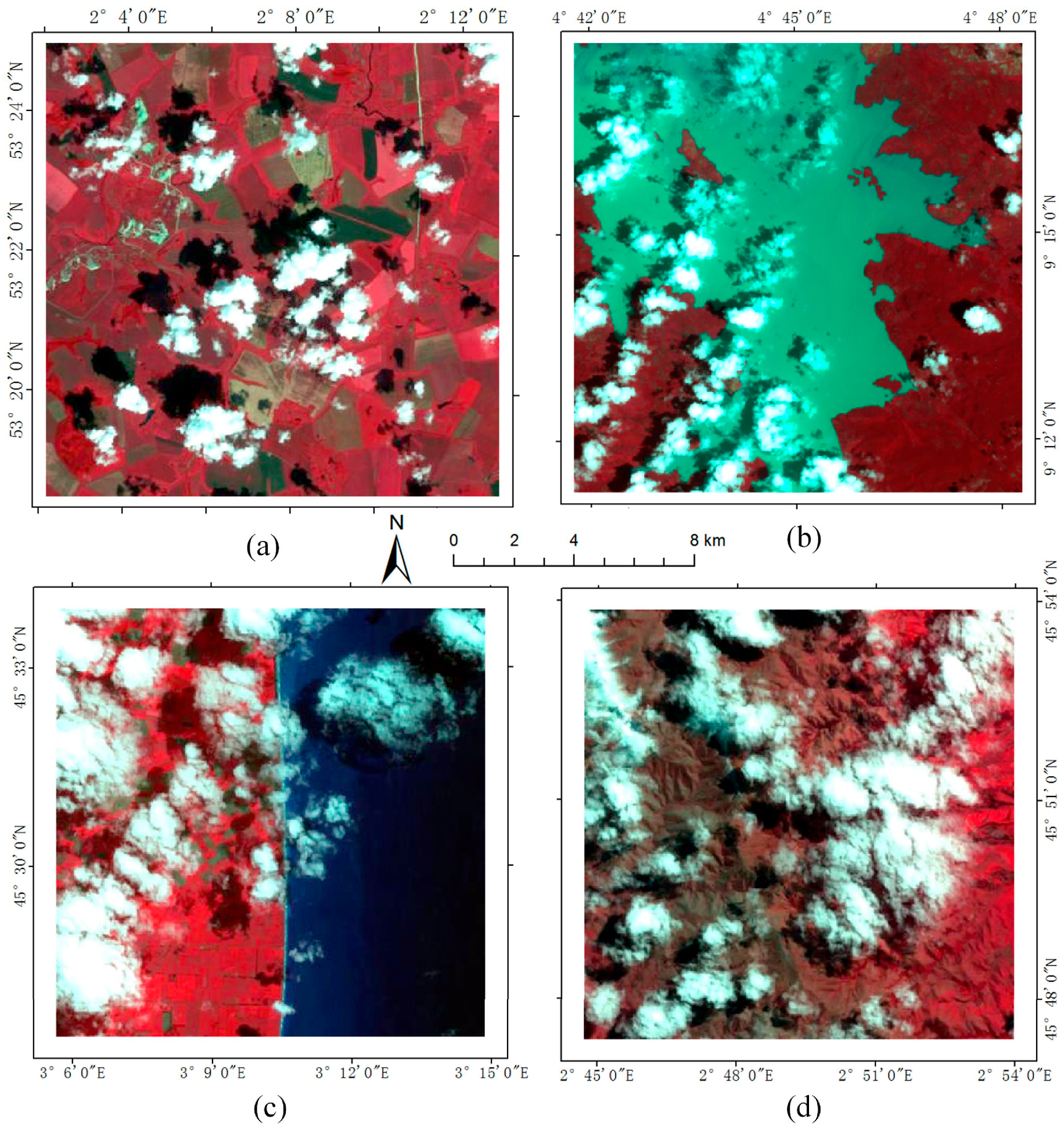
These images contain various underlying surface environment such as green vegetation, water (river and sea), building, bare rock and so on. We can easily distinguish vegetation and bare rock from cloud pixels based on their spectra properties. However, it is difficult to distinguish building and snow from clouds by spectral characteristics alone. In addition, since the semitransparent thin cloud has always been mixed with other background objects and has no clear outline, it is more difficult to detect thin cloud than thick cloud [35]. Four cloudy images with various underlying surfaces are shown in Figure 1.
2.2. Preprocessing: Feature Selection
Cloud is an aerosol comprising a visible mass of minute liquid droplets or frozen crystals, and shows cluster-like distributions in remote sensing imagery. It is generally known that the spectral reflectance value of cloud is relatively larger than those of other underlying surfaces [36]. However, because of different objects with similar spectral profiles and image noises, spectral features are not enough for cloud detection. Therefore, for high-accuracy cloud detection, we adequately consider both the spectral and spatial information of remote sensing imagery in this paper, mainly including spectral, texture and structure features [37,38].
2.2.1. Selection of Spectral Features
Cloud types vary widely, but the characteristic of cloud is generally white, bright, and cold compared to the Earth’s surface. Just as Table 3 shows, only blue (0.45–0.52 µm), green (0.52–0.59 µm), red (0.63–0.69 µm), and near infrared (0.77–0.89 µm) bands of the GF-1 images and all bands of Landsat ETM+ are used in our experiments while panchromatic bands are excluded.
2.2.2. Selection of Texture Features
Texture reflects the spatial arrangement of spectral information, which is an important portion of spatial feature [39]. In this paper, we take four frequently used texture features: means, homogeneity, second moment and correlation based on the Grey Level Co-occurrence Matrix (GLCM). In addition, as infrared band is always different from or even opposite to other bands, only the texture features of the mean of visible image bands are considered. The formulation of the four texture features we used in this paper are shown as following:
- (a)
- Meanswhere is the value in the cell in the co-occurrence matrix and is the max spectral value. Means reflects the regularity of image texture.
- (b)
- Homogeneityis the measurement of image uniformity in the local region.
- (c)
- Second momentis the image energy, and reflects the image uniformity.
- (d)
- Correlationwhere is the normalized value of co-occurrence matrix, , , , and . Measures the similarity of GCLM in the row or column direction.
2.2.3. Selection of Structure Features
Just as [40] shows, structure features describe the core information about image. The overall structure features, rather than the individual details, are always the primary information of human perception on image. To exploit structure image S for an input image I, a relative total variation (RTV) model will be employed.
where is a small constant, represents the total number of image, and is a presetting parameter for balance. and are the general pixel-wise windowed total variation measure. They represent the absolute spatial difference within the window and could be written as
where belongs to a window . () and () respectively calculate the partial derivative in and directions of image . is a weighting function, and it is defined as
and are defined as different from and ; they are written as
In our work, we set the parameter = 0.05, and use the mean values of the visible bands as inputs. Then, the right of Equation (5) is minimized to obtain the overall structure map.
3. Methodology: FAEM for Cloud Detection
The framework of the proposed method is shown in Figure 2. Three major steps were performed in this section for accurate cloud detection: (1) fundamental feature fusion; (2) deep discriminative feature learning; and (3) cloud degree prediction. The initial step of FAEM was to calculate fundamental features from the original images. During the deep feature learning phase, the selected fundamental features were fed into the established stacked autoencode networks to generate a set of feature extractors. In the final step, the membership function was used for cloud degree prediction.
3.1. Fundamental Feature Fusion
Accurate cloud detection needs to consider both spectral and spatial information. In our experiments, the spectral information is obtained from the observed band values and the spatial information is calculated according to Section 2.2. After that, they are fused to be fundamental feature vector as the input of our FAEM model. We call the fused feature as fundamental feature in this paper as it is the combination of some basic information.
In this paper, multi-type feature fusion method is chosen [41]. We regard the spectral features as for Landsat images. For GF-1 images, are spectral features. are texture features and is structure feature. All the features are combined from head to tail or . is the fundamental feature vector for the cloud detection model.
3.2. Deep Discriminative Feature Learning
The traditional artificially designed features cannot accurately represent the complex real environment. Most traditional cloud detection methods mainly focus on the construction of features to efficiently differentiate the cloud from others. In most cases, these features are “knowledge-driven”, which means they are designed artificially based on prior knowledge.
Deep learning shows that the learned deep feature has powerful ability for feature representation. Recently, deep learning has achieved much success in image processing thanks to its deep network, which is constructed with many network layers and has the ability to mine the deep discriminative feature of image. In this paper, we apply stacked autoencode networks to learn the deep discriminative feature, which is a powerful representation of corresponding sample for accurate cloud detection, with a number of samples from the real environment.
Imagine that each fundamental feature vector is a point in , and our goal is to find a function that maps each feature vector into so that the new transformed vector can be classified linearly. Suppose the feature vectors are denoted as , where is number of the training samples. The feature matrix is normalized to [0, 1] with following formulation:
where is the normalized data, and are the maximum and minimum values of the original data set.
During the feature learning stage, is the input of the network’s first layer. Formally, the output of the first layer is represented as an operation :
where and represent the weights and biases, respectively, and “” denotes the multiplication. Here, corresponds to filters of support , where is the dimension of input samples and is the dimension of the first layer output of the network. Intuitively, applies matrix multiplications on the features, and each multiplication has a size . The output is composed of -dimensional features. is an -dimensional vector, whose each element is associated with a filter. We apply the ReLU function on the filters responses. The first layer extracts the -dimensional features for each sample.
In the second layer, each of these -dimensional feature vectors is mapped to -dimensional ones. This is equivalent to applying filters which have a support . The output of the second layer is:
where contains filters of size , and is an -dimensional bias vector. The output -dimensional is the feature of the sample in anther space where the sample is easier to be classed and detected.
It is possible to add more feature learning layers to increase the non-linearity and the ability of feature representation. Nevertheless, this will increase the complexity of the model, and thus demands more computation time. We will explore deeper structures by introducing additional non-linear mapping layers in Section 4.1.
3.3. Cloud Degree Prediction
Cloud in remote sensing imagery varies spatially, and thick and thin clouds can exist in the same imagery. Most traditional methods regard cloud detection as a 0–1 classification problem by artificially selecting features and classification. However, these sample classification methods are heavily stretched to represent the real situation. In the FAEM proposed in this paper, a membership function was utilized to detect the thickness degree of the cloud at the tail of the last layer of stacked autoencode networks. The Gaussian-type membership function
is utilized in this model, where and are the parameters of the model, and the result is the degree of the training samples belonging to class , called the membership degree of . The output cloud degree of each pixel is within [0, 1], where the higher the cloud degree is, the denser the cloud is at the location of corresponding pixel. According to the output membership degree, we can further obtain the corresponding cloud density map, which shows the cloud density of each pixel on the image.
3.4. Parameter Tuning
Learning the mapping function for cloud detection requires the estimation of network parameters . This is achieved through minimizing the loss between the model output (the predicted labels) and the true labels. Given a set of pixels and their corresponding labels , the mean squared error (MSE) is used as the loss function:
where is the number of training samples.
The loss function is minimized using batch stochastic gradient descent algorithm with the standard back propagation scheme. In particular, the weight matrices are updated as follows
where and are the indices of the layers and iterations, is the learning rate, is the momentum factor, and is the derivative. The filter weights of each layer are initialized by drawing randomly from Gaussian distribution with zero mean and standard derivation 0.001 (and 0 for biases). The learning rate is 0.01 and the momentum factor is 0.9. In addition, to avoid over-fitting problem, dropout factor 0.5 is used to randomly reduce a half features during training stage. Once the model is trained, the parameters are set to construct a nonlinear mapping for discriminative feature extraction and cloud density map prediction.
3.5. Accuracy Assessment
Both qualitative and quantitative assessments are necessary. Qualitative assessment can be evaluated with visual effects. For quantitative assessment, as many other cloud detection methods (SVM, RF, Function of Mask (Fmask) [15], etc.), simply divide the imagery into two classes: cloud and non-cloud. Therefore, though the final output of our FAEM is a cloud density map, for the convenience of assessment, we convert it into cloud and non-cloud for quantitative comparison with other methods.
In addition to overall accuracy (OA) and Kappa, there are four metrics used in this paper: right rate (RR), error rate (ER), false alarm rate (FAR), and the ratio of RR to ER (RER). RR is defined as
where CC is the number of correctly detected cloud pixels and GN is the number of cloud pixels in ground truth. RR provides us with the information of correctly detected results.
ER is defined as [42]
where CN represents the number of cloud pixels identified as non-cloud pixels. NC represents the number of non-cloudy pixels identified as cloud pixels, and TN denotes the number of pixels of the input image. ER is used to provide incorrect information.
FAR is defined with the same form as in the papers [37]
where NC and TN have the same meanings as the above formula. FAR is one part of ER and it explicitly represents the false alarm rate.
Using only one of them to assess algorithms is insufficient, as some methods may obtain high RR but bring too many false alarms. On the contrary, some methods may obtain low ER but also low RR. Therefore, RER is defined to obtain an integrated result as it considers the RR and ER. The higher it is, the better it will be. RER is defined as the ratio of RR to ER
4. Experiments and Results
As there are some adjustable parameters in our FAEM model, we first analysis and determine the best parameter combination for accurate detection result. In this experiments, 16,698 cloud pixels and 50,253 non-cloud pixels which contain as many objects as possible are selected as samples for the Landsat ETM+ imagery. The numbers of cloud and non-cloud samples for 25 GF-1 images are 13,197 and 17,462 respectively. In addition, the samples should belong to the pure objects such as thick cloud, water, building, vegetation and so on, the thin cloud which is actually the mixture of cloud and ground objects is not selected as samples.
After that, the samples are divided into two parts: training set and test set, and the number of training and test set are 2/3 and 1/3 of the total number of samples respectively. During the training procedure, training set is used for model training and after each training epoch, the test sets are used to test the trained model and output the corresponding test accuracy. At the prediction procedure, each pixel’s degree of belonging to cloud is predicted and used to derive the corresponding cloud density map. Moreover, to demonstrate the efficiency of proposed model, both Landsat ETM+ and GF-1 images with different spatial resolution are applied in this experiment.
4.1. Parameter Analysis
The number of layers and hidden nodes can influence the result of cloud detection. In our previous experiments with Landsat ETM+ imagery, the number of the fundamental vector is 13 (including spectral, texture and structural information) and the numbers of the two hidden layers are 12 and 10, respectively, and a cloud density map is outputted as last. For convenience, we denote the model node number as 13-12-10-1. In this section, several experiments are designed to fully explore the relation between different model parameter combinations and cloud detection results.
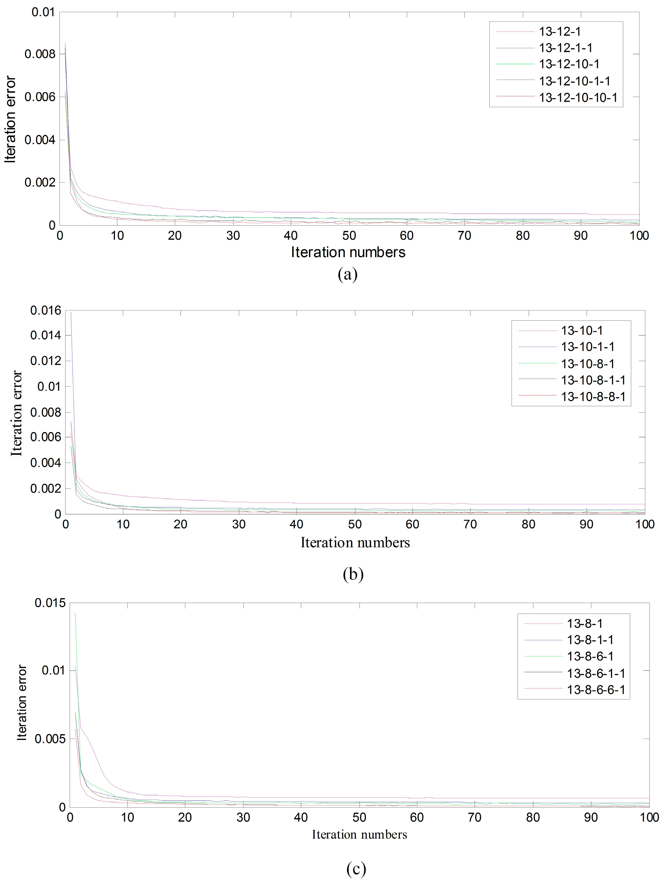
Based on our model parameters set in Section 3.2, we conduct four groups of experiments in this section. The trend of iteration error and the iteration number are reported in Figure 3. In experiment (a), by comparing experiments with node number 13-12-1, 13-12-10-1 and 13-12-10-10-1, we can see that the convergent rate is getting quicker and the final iteration error is becoming lower with the increase of the model layers. Similarly, experiments (b) and (c) demonstrate the same regular pattern. In addition, it also shows that when the model layers increase from 3 to 4, the final iteration error falls along with it. At the same time, the final iteration error with 4 and 5 model layers are basically equal, while the computational complexity can be raised. Therefore, we focus on the relation of model performance and the number of hidden nodes with 4 model layers. Figure 3d exhibits the results with different number of hidden nodes, which shows that model 13-12-10-1 has acquired relatively better performance for our cloud detection issue.
4.2. Experiment on Landsat ETM+ Imagery
4.2.1. Cloud Density Map Predication
In this section, we give some qualitative prediction results with our model. According to the parameter analysis in Section 4.1, we set the parameter combination of the FAEM for Landsat ETM+ imagery to be 13-12-10-1. The parameters and (in Section 3.3) in the membership function are set as 3 and 1, respectively.
Figure 4 shows the predicted cloud density map two randomly selected experimental images. The left column represents the original Landsat ETM+ images. The images in the second column are corresponding cloud density map. It can be seen that either thin cloud or thick cloud have been detected very well with our proposed FAEM. In addition, for images that contain many ma-made objects, which have similar spectral characteristics with clouds, the proposed model can still precisely detect the cloud without being affected.
4.2.2. Comparison with Other Methods
As most traditional methods regard the cloud detection as 0–1 classification problem [43,44,45], the classification results only contain cloud and non-cloud. For the convenience of quantitative comparison, we use a threshold 0.5 to cut the pixels whose cloud degrees in density map are smaller than the threshold to be non-cloud and the remains are regard as clouds. In this experiment, Landsat ETM+ images are considered to demonstrate the effectiveness of proposed approach.
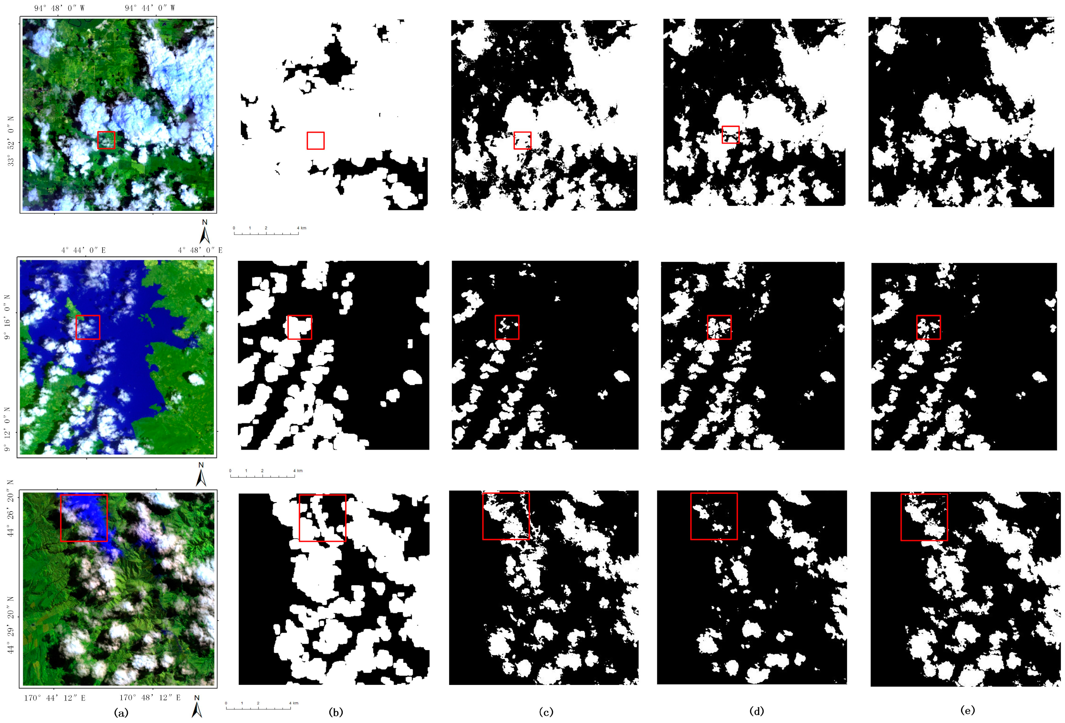
In this experiment, we use 172 Landsat ETM+ images with manual labelled as ground truth and the results are compared with some other cloud detection methods such as Fmask, SVM and RF. Figure 5 shows the detection results of three images containing different underlying surfaces with different methods. Results show that regardless of images with vegetation (first row), water (second row) or snow (third row), the proposed method has shown stronger stability and better performance than Fmask, SVM and RF for cloud detection. Obviously, Fmask is seriously overestimated in the three images. For images with extensive vegetation in the first row, SVM is much more likely to detect some bright ground objects as cloud. While in the second-row images with water, SVM confuses some cloud as non-cloud. In particular, for the third-row images with snow, which is a challenging case in cloud detection since snow and cloud also have similar characteristics on remote sensing image, both SVM and RF obtain false results in such circumstance, SVM has regarded much more ice as cloud while RF only detects a part of the cloud from the snow.
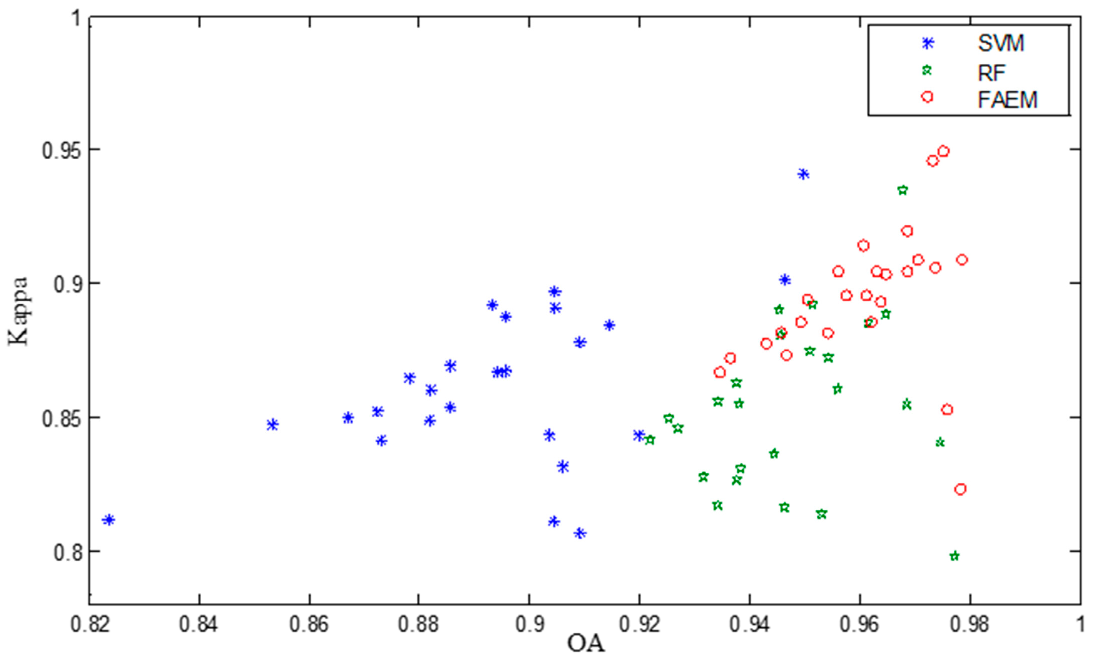
Figure 6 exhibits the Kappa and OA of 172 Landsat ETM+ images with Fmask, SVM, RF and proposed approach. The Kappa and OA for our proposed method, which are lying in the upper right corner, are dramatically higher than others. By comparison, the performance of Fmask is slightly unsatisfactory. The result of SVM and RF is very close, and most of their OA and Kappa are higher than 0.9 and 0.8 respectively.
To further compare the detection results, four evaluation indicators RR, ER, FAR and RER are calculated in this experiment. The average results of 172 Landsat ETM+ images are shown in Table 4. We can see that for Fmask, RR is closer to 1, ER and FAR are 10 times larger than others, and the RER is least among all methods. This shows the performance of Fmask is overestimated: many non-cloud are regarded as cloud pixels. Meanwhile, the RR of our proposed method is high up to 0.86, which is more than SVM and RF, while the ER of the proposed method is much smaller. More importantly, the RER of our method is high, up to 29.50, while it is only 10.984, 21.84 and 23.02 for Fmask, SVM and RF, respectively.
4.3. Experiments on GF-1 Imagery
4.3.1. Cloud Density Map Predication
To demonstrate that the proposed model is available for different imagery with different spatial resolutions, GF-1 imagery with 8 m spatial resolution is also be considered in this section. The fundamental vector dimension of GF-1 imagery is 9 (including spectral, texture and structure information) in this experiment. Similar to the parameter analysis in Section 4.1, we set the model parameter combination for GF-1 imagery to be 9-8-6-1. The parameters and (in Section 3.3) in the membership function are set as 3 and 1 respectively, which is the same with Landsat ETM+ imagery.
Similar as the experiments on Landsat ETM+ imagery, two randomly selected images and their corresponding detection results are shown in Figure 7. The left column represents the original GF-1 images and the images in second column are their corresponding cloud density map. It shows that for GF-1 imagery with higher spatial resolution, the proposed model still work well for accurate cloud detection. In Figure 7, we can see that both thin cloud and thick cloud have been well detected. Larger value represents that the pixels contains more cloud composition. For the value equals to 1, it means that the pixel is pure cloud. Conversely, the smaller the value is, the thinner the cloud is likely to be at the point.
4.3.2. Comparison with Other Methods
Twenty-five GF-1 images are considered in this experiment. To save space, we display only three groups of detection results with different methods. Figure 8 shows the pseudo color images combined with band 4, 3, and 2. Clouds in these images have quite different shapes and thicknesses. From the left to right of Figure 8, it shows original image and the detection results with SVM, RF and the proposed method, respectively. For images with extensive mountainous area, all three methods have acquired relatively satisfactory detection results. However, when there are many buildings and roads in the image, SVM and RF, which simply use artificially designed primary features, have difficulty. The advantage of our proposed method is well shown in this case.
In Figure 9, we can see the Kappa and OA of cloud detection results on GF-1 images. Most of our results appear in the upper right corner. It shows that higher accuracy can be achieved in our method.
After the previous qualitative comparison, we now focus on a quantitative comparison of our method as shown in Table 5. Similar with the analyses of Landsat ETM+ images, the four same evaluation indicators RR, ER, FAR and RER are used for GF-1 assessment. It can be seen from Table 5 that our proposed method has acquired much higher right rate than SVM and RF, while the error rate of the proposed method is much smaller. In particular, The RER with our method is high, up to 25.94, while for SVM and RF it is only 19.15 and 17.75, respectively.
5. Discussion
5.1. Analysis of Feature Combination
In this section, experimental results with three different feature combinations of spectra, spectra + texture and spectra + texture + structure are reported. Three Landsat images containing thick cloud and thin cloud of different surface earth are considered. As Figure 10 shows, from left to right, the cloud detection results with feature combinations of spectra, spectra + texture and spectra + texture + structure are listed. Compared with the original images, we can see that the detection results become better along with the increasing of features.
Table 6 illustrates the ER, RR, FAR and RER of testing images with different feature combinations. Obviously, the values of RR and RER increase along with the number of features, while the ER values decrease.
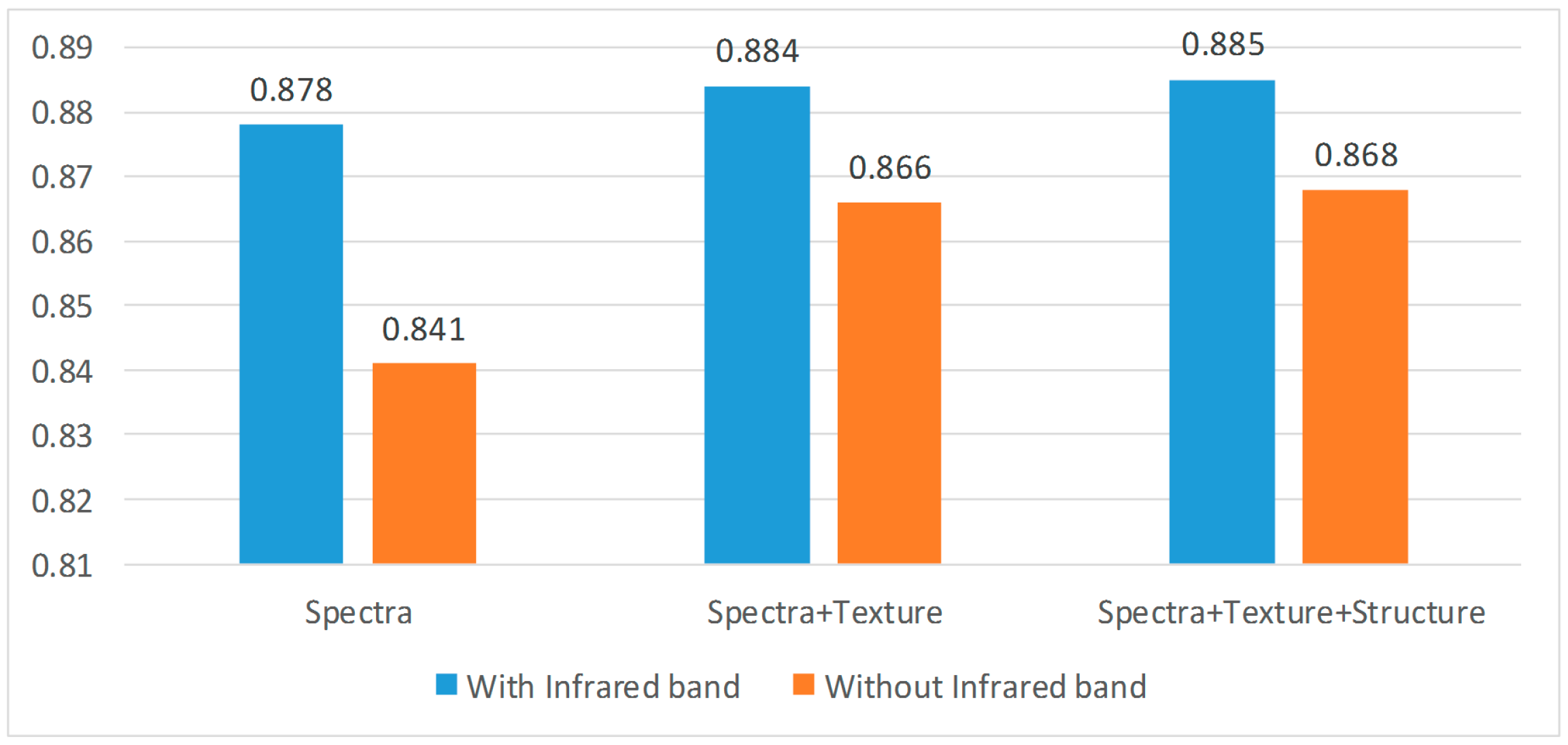
5.2. Analysis of Bands Necessity
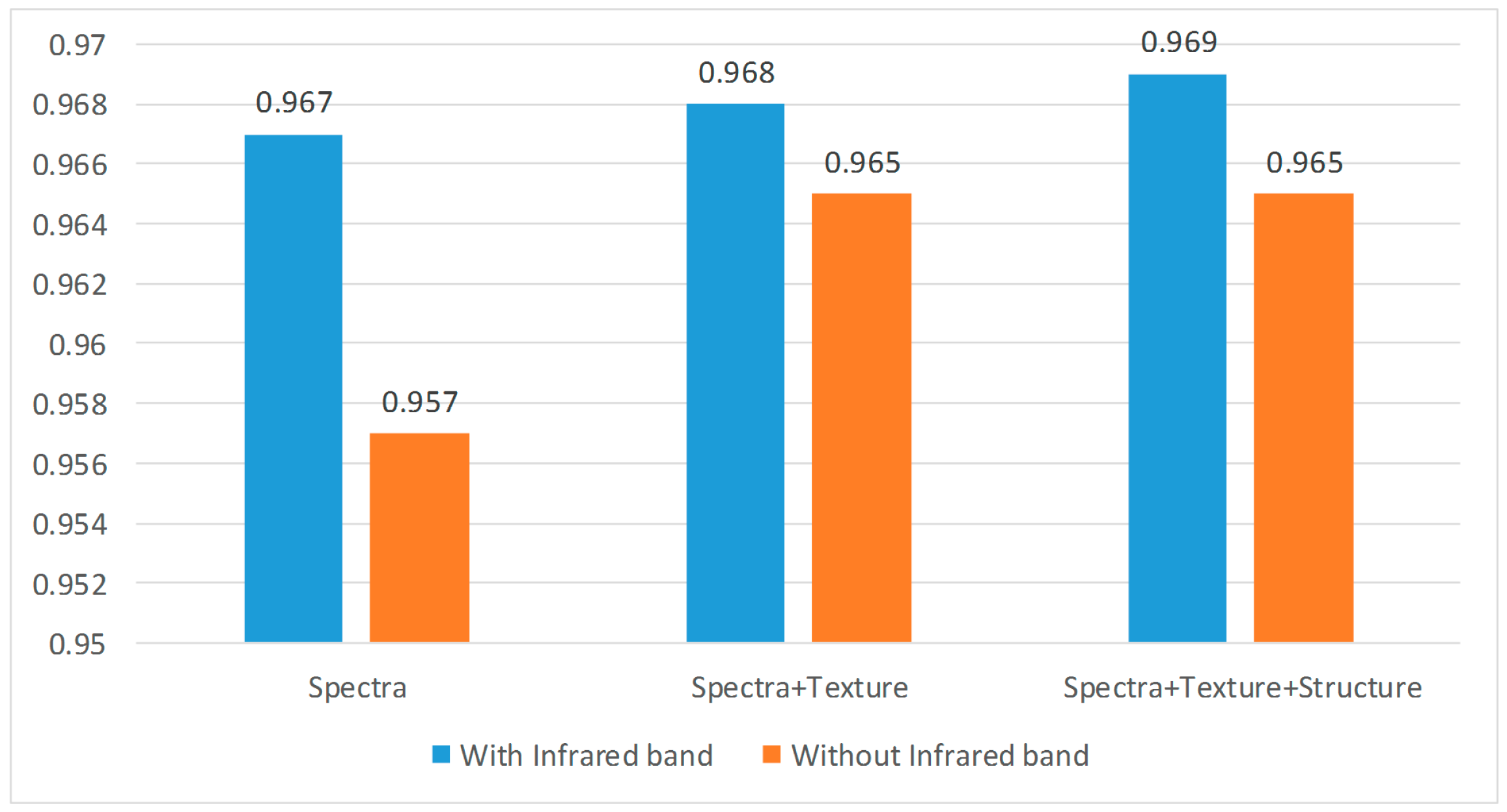
In our pervious experiments, both visible band and infrared band are considered. However, cloud has high reflectance in visible band while its reflectance in infrared band is low. Due to the characteristics of high light and low temperature, cloud commonly shows different characteristics in visible and infrared bands. In this section, we aim to explore the effects of the infrared band for cloud detection.
Similar to Section 5.1, different feature combinations of spectra, spectra + texture, spectra + texture + structure are considered in the experiments. Nonetheless, we remove the infrared band in the experiments for comparison. Table 7 shows the average value of four metrics of 172 experiment Landsat ETM+ images. Compared with the experiments using all bands in Section 5.1, the detection accuracy with feature combination of spectra + texture and spectra + texture + structure do not change much, while, for experiments that only consider the spectral information, infrared band plays a relatively important role.
For a clearer comparison, Figure 11 and Figure 12 show the average Kappa and OA of the 172 experimental Landsat ETM+ images respectively. The blue bars represent the experimental accuracy using all bands and the red bars are the detection accuracy without infrared band. Data in Figure 11 and Figure 12 also show the same conclusion that the infrared band is necessary for cloud detection with only spectral information. As for experiments combined with spatial information (texture and structure), which constrains the spatial consistency of the detection result, the influence of infrared band becomes weak.
6. Conclusions
This study has presented a new cloud detection method. The advantages of the proposed method are integrating the feature learning ability of stacked autoencode networks and the detection ability of fuzzy function to acquire good performance on cloud detection. To validate the effectiveness of our method, 172 Landsat ETM+ images and 25 GF-1 images are used in this paper. Experimental results demonstrate that the proposed approach has achieved relatively higher detection accuracy compared with several state-of-the-art cloud detection methods (Fmask, SVM, and RF). Furthermore, we experimentally demonstrate that feature combination of spectral + texture + structure has attained better performance than single feature. Our proposed method is applicable in a variety of scenarios and is reliable in different resolution images. Generally, the proposed approach can potentially yield better results in terms of detection accuracy compared with related approaches, and is not limited by image resolution.
To fully consider the spatial and spectral information for a better cloud detection result, three fundamental features, spectral, texture and structure features, are applied in this work as the basic information to learn a deep discriminative feature. However, these texture and structure features are still manually selected and may not contain enough information. In future study, we will consider applying convolutional network for cloud detection. In addition, as convolutional network extracts feature with convolution kernel by integrating the local spatial information, the global constraint information will also be combined for accurate cloud detection.
Acknowledgments
This work was supported by the National Key Technologies Research and Development Program (2016YFB0502603); Fundamental Research Funds for the Central Universities (2042016kf0179 and 2042016kf1019); Guangzhou science and technology project (201604020070); National Administration of Surveying, Mapping and Geoinformation (2015NGCM); Wuhan Chen Guang Project (2016070204010114); and Special task of technical innovation in Hubei Province (2016AAA018).
Author Contributions
Zhenfeng Shao, Juan Deng and Lei Wang conceived and designed the framework of this research; Juan Deng performed the experiments; Lei Wang, Yewen Fan, Qimin Cheng and Neema S. Sumari gave some advices in writing the paper; and Juan Deng wrote the paper.
Conflicts of Interest
The authors declare no conflict of interest.
References
- Lv, H.; Wang, Y.; Shen, Y. An empirical and radiative transfer model based algorithm to remove thin clouds in visible bands. Remote Sens. Environ. 2016, 179, 183–195. [Google Scholar] [CrossRef]
- Xu, X.C.; Liu, X.P.; Li, X.; Xin, Q.C.; Chen, Y.M.; Shi, Q.; Ai, B. Global snow cover estimation with microwave brightness temperature measurements and one-class in situ observations. Remote Sens. Environ. 2016, 182, 227–251. [Google Scholar] [CrossRef]
- Zhu, Z.; Wang, S.; Woodcock, C.E. Improvement and expansion of the fmask algorithm: Cloud, cloud shadow, and snow detection for landsats 4–7, 8, and sentinel 2 images. Remote Sens. Environ. 2015, 159, 269–277. [Google Scholar] [CrossRef]
- Bian, J.H.; Li, A.N.; Jin, H.A.; Zhao, W.; Lei, G.B.; Huang, C.Q. Multi-temporal cloud and snow detection algorithm for the hj-1a/b ccd imagery of china. In Proceedings of the 2014 IEEE International Geoscience and Remote Sensing Symposium (IGARSS), Quebec City, QC, Canada, 13–18 July 2014; pp. 501–504. [Google Scholar]
- Hagolle, O.; Huc, M.; Pascual, D.V.; Dedieu, G. A multi-temporal method for cloud detection, applied to formosat-2, venµs, landsat and sentinel-2 images. Remote Sens. Environ. 2010, 114, 1747–1755. [Google Scholar] [CrossRef]
- Tang, H.R.; Yu, K.; Hagolle, O.; Jiang, K.; Geng, X.R.; Zhao, Y.C. A cloud detection method based on a time series of modis surface reflectance images. Int. J. Digit. Earth 2013, 6, 157–171. [Google Scholar] [CrossRef]
- Jin, S.M.; Homer, C.; Yang, L.M.; Xian, G.; Fry, J.; Danielson, P.; Townsend, P.A. Automated cloud and shadow detection and filling using two-date landsat imagery in the USA. Int. J. Remote Sens. 2013, 34, 1540–1560. [Google Scholar] [CrossRef]
- Goodwin, N.R.; Collett, L.J.; Denham, R.J.; Flood, N.; Tindall, D. Cloud and cloud shadow screening across queensland, australia: An automated method for landsat tm/etm plus time series. Remote Sens. Environ. 2013, 134, 50–65. [Google Scholar] [CrossRef]
- Zhu, Z.; Woodcock, C.E. Automated cloud, cloud shadow, and snow detection in multitemporal landsat data: An algorithm designed specifically for monitoring land cover change. Remote Sens. Environ. 2014, 152, 217–234. [Google Scholar] [CrossRef]
- Marais, I.V.; Du Preez, J.A.; Steyn, W.H. An optimal image transform for threshold-based cloud detection using heteroscedastic discriminant analysis. Int. J. Remote Sens. 2011, 32, 1713–1729. [Google Scholar] [CrossRef]
- Shao, Z.; Hou, J.; Jiang, M.; Zhou, X. Cloud detection in landsat imagery for antarctic region using multispectral thresholds. SPIE Asia-Pac. Remote Sens. Int. Soc. Opt. Photonics 2014. [Google Scholar] [CrossRef]
- Bley, S.; Deneke, H. A threshold-based cloud mask for the high-resolution visible channel of meteosat second generation seviri. Atmos. Meas. Tech. 2013, 6, 2713–2723. [Google Scholar] [CrossRef]
- Zhu, T.T.; Wei, H.K.; Zhang, C.; Zhang, K.J.; Liu, T.H. A local threshold algorithm for cloud detection on ground-based cloud images. In Proceedings of the 34th Chinese Control Conference, Hangzhou, China, 28–30 July 2015; pp. 3702–3706. [Google Scholar]
- Irish, R.R. Landsat 7 automatic cloud cover assessment. Proc. SPIE Int. Soc. Opt. Eng. 2000, 4049, 348. [Google Scholar] [CrossRef]
- Zhu, Z.; Woodcock, C.E. Object-based cloud and cloud shadow detection in landsat imagery. Remote Sens. Environ. 2012, 118, 83–94. [Google Scholar] [CrossRef]
- Qing, Z.; Chunxia, X. Cloud detection of rgb color aerial photographs by progressive refinement scheme. IEEE Trans. Geosci. Remote Sens. 2014, 52, 7264–7275. [Google Scholar] [CrossRef]
- Tan, K.; Zhang, Y.; Tong, X. Cloud extraction from chinese high resolution satellite imagery by probabilistic latent semantic analysis and object-based machine learning. Remote Sens. 2016, 8, 963. [Google Scholar] [CrossRef]
- Choi, H.; Bindschadler, B. Cloud detection in landsat imagery of ice sheets using shadow matching technique and automatic normalized difference snow index threshold value decision. Remote Sens. Environ. 2004, 91, 237–242. [Google Scholar] [CrossRef]
- Xu, D.; Qu, J.J.; Niu, S.; Hao, X. Sand and dust storm detection over desert regions in china with modis measurements. Int. J. Remote Sens. 2011, 32, 9365–9373. [Google Scholar] [CrossRef]
- Surya, S.R.; Simon, P. Automatic cloud detection using spectral rationing and fuzzy clustering. In Proceedings of the 2013 Second International Conference on Advanced Computing, Networking and Security (Adcons 2013), Mangalore, India, 15–17 December 2013; pp. 90–95. [Google Scholar]
- Liang, S.L.; Fang, H.L.; Chen, M.Z. Atmospheric correction of landsat etm+ land surface imagery—Part I: Methods. IEEE Trans. Geosci. Remote Sens. 2001, 39, 2490–2498. [Google Scholar] [CrossRef]
- Xu, L.; Niu, R.; Fang, S.; Dong, Y. Cloud detection based on decision tree over tibetan plateau with modis data. Proc. SPIE Int. Soc. Opt. Eng. 2013, 8921, 89210G. [Google Scholar] [CrossRef]
- Ren, R.Z.; Gu, L.J.; Wang, H.F. Clouds and clouds shadows detection and matching in modis multispectral satellite images. In Proceedings of the 2012 International Conference on Industrial Control and Electronics Engineering (ICICEE), Xi’an, China, 23–25 August 2012; pp. 71–74. [Google Scholar]
- Kong, X.; Qian, Y.; Zhang, A. Cloud and shadow detection and removal for landsat-8 data. Proc. SPIE Int. Soc. Opt. Eng. 8921, 8921, 89210N. [Google Scholar] [CrossRef]
- Rumi, E.; Kerr, D.; Coupland, J.M.; Sandford, A.P.; Brettle, M.J. Automated cloud classification using a ground based infra-red camera and texture analysis techniques. SPIE Remote Sens. Int. Soc. Opt. Photonics 2013, 8890, 88900J. [Google Scholar] [CrossRef]
- Liu, L.; Sun, X.; Chen, F.; Zhao, S.; Gao, T. Cloud classification based on structure features of infrared images. J. Atmos. Ocean. Technol. 2011, 28, 410–417. [Google Scholar] [CrossRef]
- Zheng, H.; Wen, T.; Li, Z. A cloud detection algorithm using edge detection and information entropy over urban area. Eighth Int. Symp. Multispectr. Image Process. Pattern Recognit. Int. Soc. Opt. Photonics 2013, 8921, 892104. [Google Scholar] [CrossRef]
- Fisher, A. Cloud and cloud-shadow detection in spot5 hrg imagery with automated morphological feature extraction. Remote Sens. 2014, 6, 776–800. [Google Scholar] [CrossRef]
- Li, Q.; Lu, W.; Yang, J.; Wang, J.Z. Thin cloud detection of all-sky images using markov random fields. IEEE Geosci. Remote Sens. Lett. 2012, 9, 417–421. [Google Scholar] [CrossRef]
- Alireza, T.; Fabio, D.F.; Cristina, C.; Stefania, V. Neural networks and support vectormachine algorithms for automatic cloud classification of whole-sky ground-based images. IEEE Trans. Geosci. Remote Sens. 2015, 12, 666–670. [Google Scholar]
- Latry, C.; Panem, C. Cloud detection with svm technique. IEEE Trans. Geosci. Remote Sens. 2007, 448–451. [Google Scholar] [CrossRef]
- Xiangyun, H.; Yan, W.; Jie, S. Automatic recognition of cloud images by using visual saliency features. IEEE Geosci. Remote Sens. Lett. 2015, 12, 1760–1764. [Google Scholar] [CrossRef]
- Ma, C.; Chen, F.; Liu, J.; Duan, J. A new method of cloud detection based on cascaded adaboost. IOP Conf. Ser. Earth Environ. Sci. 2014, 18, 012026. [Google Scholar] [CrossRef]
- GF-1 Images. Geospatial Data Cloud. Available online: http://www.gscloud.cn/ (accessed on 8 August 2016).
- Bai, T.; Li, D.R.; Sun, K.M.; Chen, Y.P.; Li, W.Z. Cloud detection for high-resolution satellite imagery using machine learning and multi-feature fusion. Remote Sens. 2016, 8, 715. [Google Scholar] [CrossRef]
- Liu, R.G.; Liu, Y. Generation of new cloud masks from modis land surface reflectance products. Remote Sens. Environ. 2013, 133, 21–37. [Google Scholar] [CrossRef]
- An, Z.Y.; Shi, Z.W. Scene learning for cloud detection on remote-sensing images. IEEE J. Sel. Top. Appl. Earth Obs. Remote Sens. 2015, 8, 4206–4222. [Google Scholar] [CrossRef]
- Li, P.; Dong, L.; Xiao, H.; Xu, M. A cloud image detection method based on svm vector machine. Neurocomputing 2015, 169, 34–42. [Google Scholar] [CrossRef]
- Zhang, H.S.; Lin, H.; Li, Y. Impacts of feature normalization on optical and sar data fusion for land use/land cover classification. IEEE Geosci. Remote Sens. Lett. 2015, 12, 1061–1065. [Google Scholar] [CrossRef]
- Aujol, J.-F.; Gilboa, G.; Chan, T.; Osher, S. Structure-texture image decomposition—modeling, algorithms, and parameter selection. Int. J. Comput. Vis. 2006, 67, 111–136. [Google Scholar] [CrossRef]
- Xiao, B.; Chuntian, L.; Peng, R.; Jun, Z.; Huijie, Z.; Yun, S. Object classification via feature fusion based marginalized kernels. IEEE Geoscie. Remote Sens. Lett. 2015, 12, 8–12. [Google Scholar] [CrossRef]
- Yuan, Y.; Hu, X.Y. Bag-of-words and object-based classification for cloud extraction from satellite imagery. IEEE J. Sel. Top. Appl. Earth Obs. Remote Sens. 2015, 8, 4197–4205. [Google Scholar] [CrossRef]
- Han, Y.; Kim, B.; Kim, Y.; Lee, W.H. Automatic cloud detection for high spatial resolution multi-temporal images. Remote Sens. Lett. 2014, 5, 601–608. [Google Scholar] [CrossRef]
- Sedano, F.; Kempeneers, P.; Strobl, P.; Kucera, J.; Vogt, P.; Seebach, L.; San-Miguel-Ayanz, J. A cloud mask methodology for high resolution remote sensing data combining information from high and medium resolution optical sensors. ISPRS J. Photogramm. Remote Sens. 2011, 66, 588–596. [Google Scholar] [CrossRef]
- Chen, Z.; Deng, T.; Zhou, H.; Luo, S. Cloud detection based on HSI color space and SWT from high resolution color remote sensing imagery. Proc. SPIE Int. Soc. Opt. Eng. 2013, 8919, 891907. [Google Scholar] [CrossRef]
Figure 1.
Cloudy images with various underlying surfaces: (a) green vegetation; (b) river; (c) coast; and (d) bare rock.
Figure 1.
Cloudy images with various underlying surfaces: (a) green vegetation; (b) river; (c) coast; and (d) bare rock.

Figure 2.
The framework of proposed method.
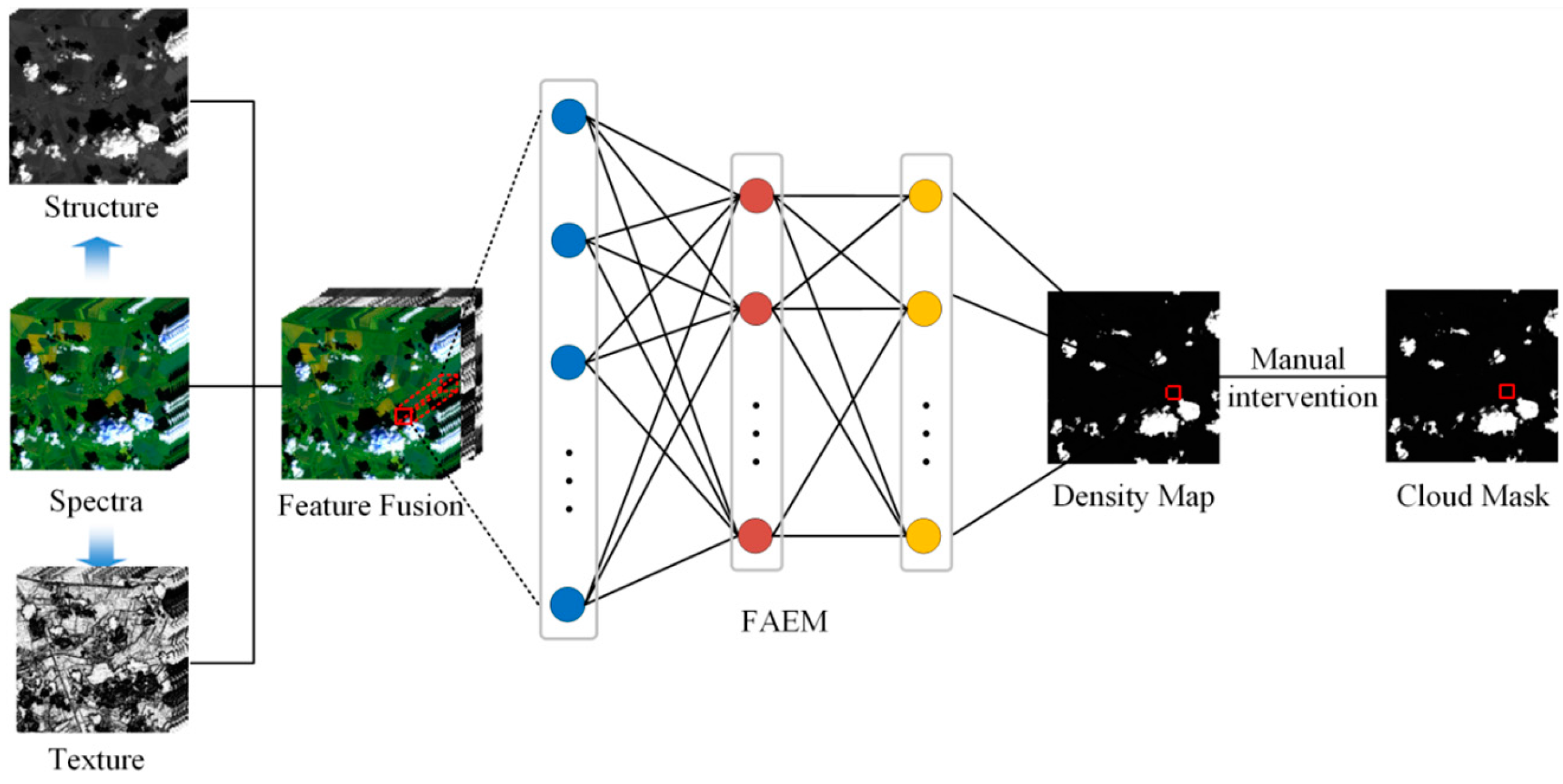
Figure 3.
(a–d) The correlation of iteration numbers and iteration error.

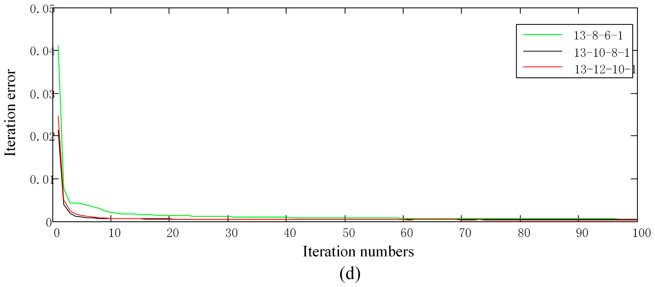
Figure 4.
(a–d): (a,c) The original image of Landsat ETM+ images; and (b,d) the corresponding cloud density.
Figure 4.
(a–d): (a,c) The original image of Landsat ETM+ images; and (b,d) the corresponding cloud density.
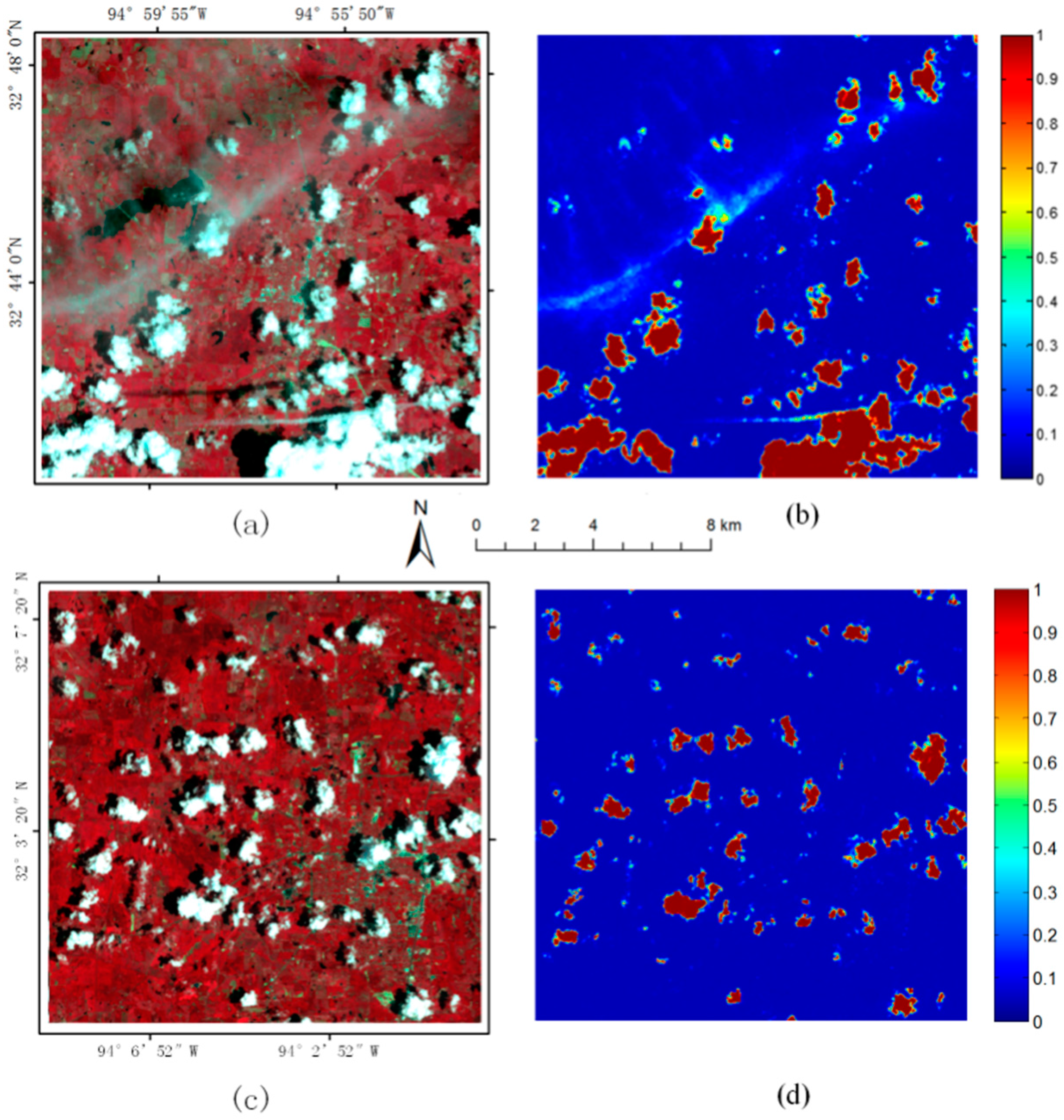
Figure 5.
(a) Pseudo color Landsat ETM+ image with Band 4 as red, Band 3 as green, and Band 2 as blue. Cloud detection results with: Fmaks (b); SVM (c); RF (d); and our proposed approach (e).
Figure 5.
(a) Pseudo color Landsat ETM+ image with Band 4 as red, Band 3 as green, and Band 2 as blue. Cloud detection results with: Fmaks (b); SVM (c); RF (d); and our proposed approach (e).

Figure 6.
Kappa and OA of 172 Landsat ETM+ images with Fmask, SVM, RF and proposed approach.
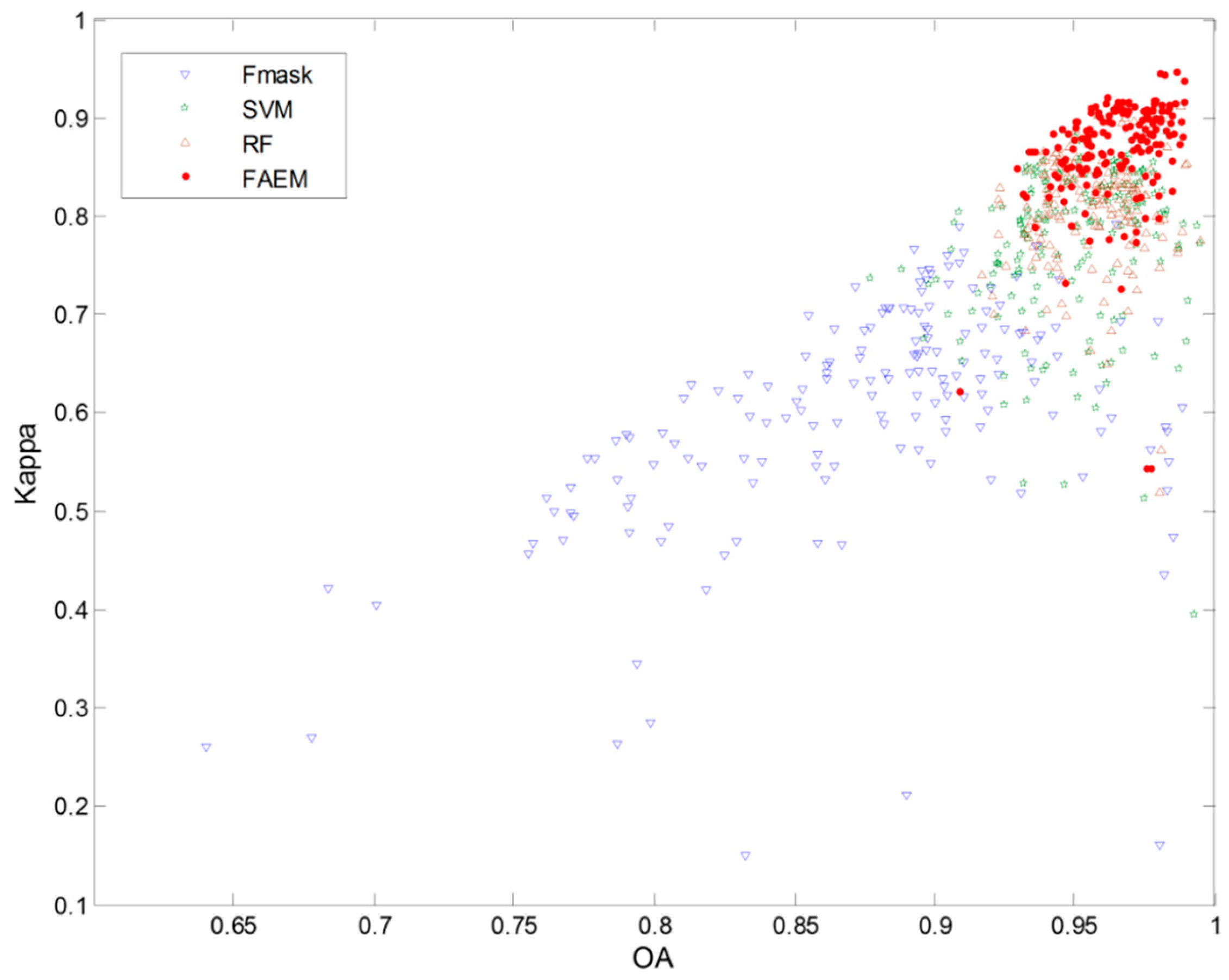
Figure 7.
(a,c) The original image of GF-1 images; and (b,d) the corresponding cloud density of (a,c) with proposed approach.
Figure 7.
(a,c) The original image of GF-1 images; and (b,d) the corresponding cloud density of (a,c) with proposed approach.
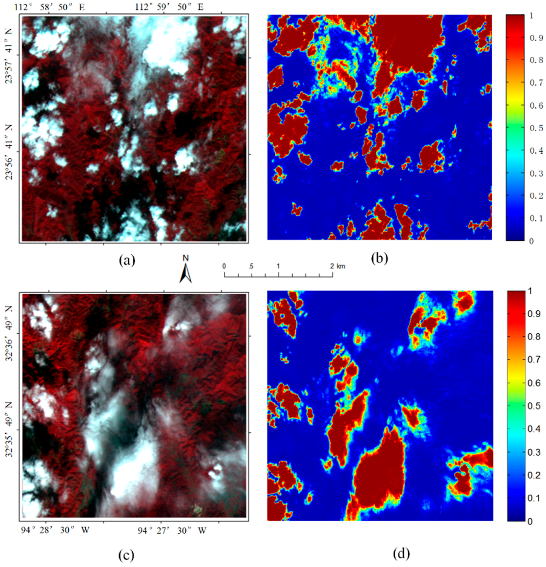
Figure 8.
(a) Pseudo color GF-1 image with combination of band 4-3-2; and (b–d) the cloud detection results with SVM, RF and our proposed approach, respectively.
Figure 8.
(a) Pseudo color GF-1 image with combination of band 4-3-2; and (b–d) the cloud detection results with SVM, RF and our proposed approach, respectively.
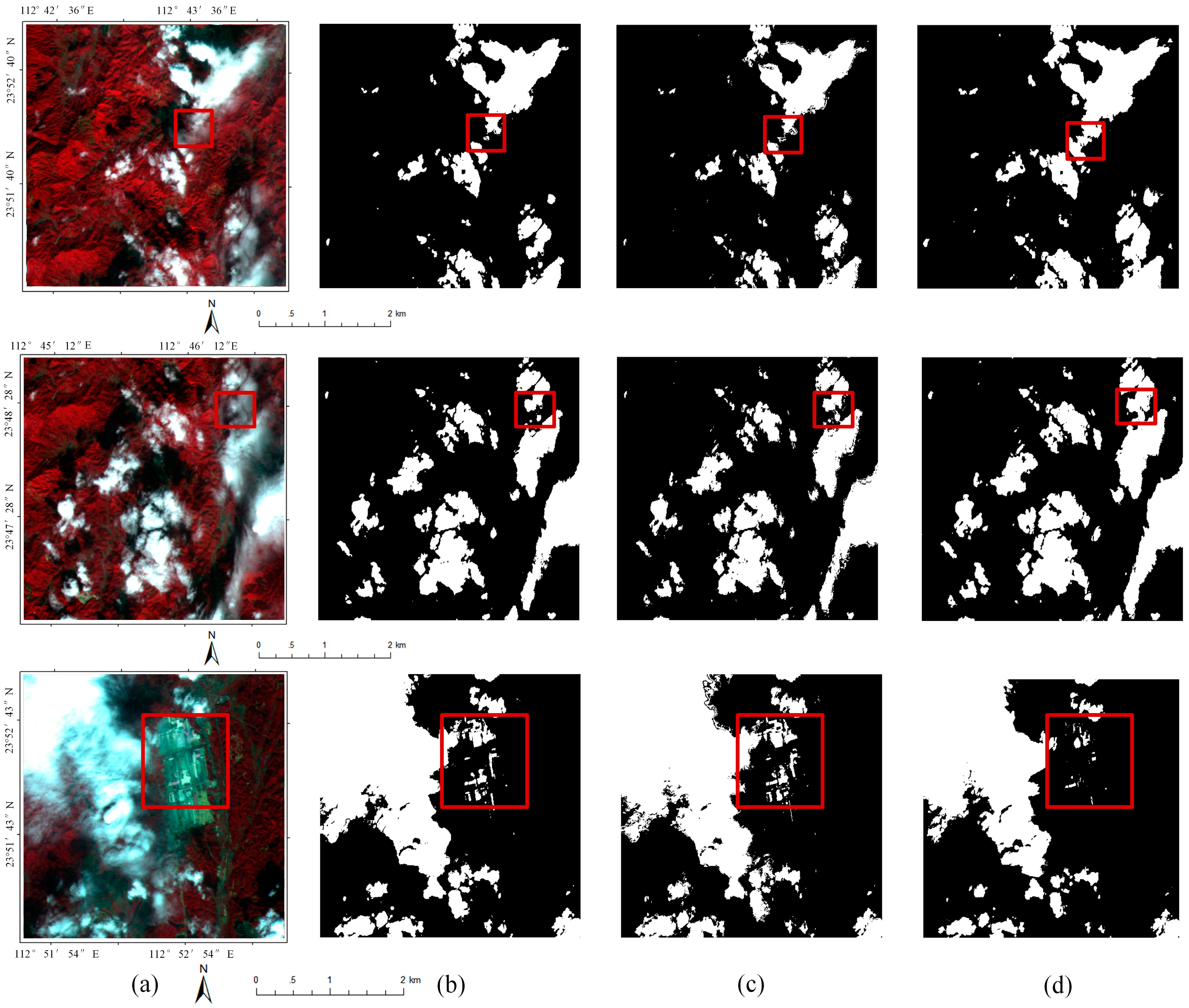
Figure 9.
Kappa and OA of 25 GF-1 images with SVM, RF and proposed approach.

Figure 10.
Visual comparisons of detection results with different fundamental features combination: (a) the original image with band combination 3-4-1; and (b–d) detected results of spectra, spectra + texture, and spectra + texture+ structure, respectively.
Figure 10.
Visual comparisons of detection results with different fundamental features combination: (a) the original image with band combination 3-4-1; and (b–d) detected results of spectra, spectra + texture, and spectra + texture+ structure, respectively.
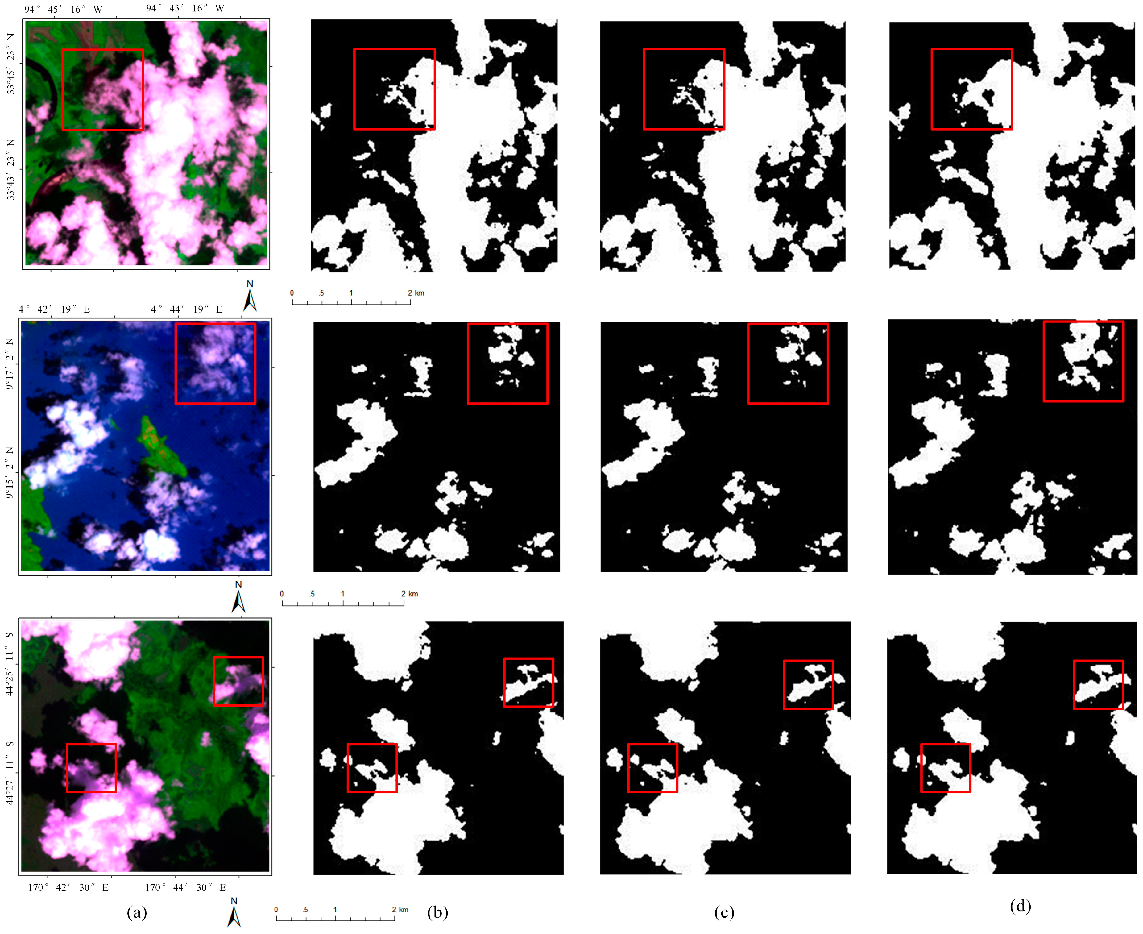
Figure 11.
Average Kappa of 172 Landsat ETM+ images with different feature combination.

Figure 12.
Average OA of 172 Landsat ETM+ images with different feature combination.

Table 1.
Detailed information of experimental data and cloud cover.
| Satellite Parameters | Landsat ETM | GF-1 |
|---|---|---|
| Product level | Level 1 | 1A |
| Number of bands | 8 | 4 |
| Spatial resolution | 30 m (60 m for infrared band) | 8m |
| Image size (pixel) | 500 × 500 | 500 × 500 |
| Acquisition time (year) | 2001 | 2014 |
| Number of images | 172 | 25 |
Table 2.
Number of images with different cloud covers.
| Cloud Cover | 0%–10% | 10%–20% | 20%–30% | 30%–40% | >40% |
|---|---|---|---|---|---|
| Landsat ETM+ | 34 | 62 | 55 | 14 | 7 |
| GF-1 | 1 | 3 | 6 | 7 | 8 |
Table 3.
Experimental data sources and bands information.
| ETM+ Bands (µm) | GF-1 (µm) |
|---|---|
| Band 1 (0.45–0.515) | Band 1 (0.45–0.52) |
| Band 2 (0.525–0.605) | Band 2 (0.52–0.59) |
| Band 3 (0.63–0.69) | Band 3 (0.63–0.69) |
| Band 4 (0.75–0.90) | Band 4 (0.77–0.89) |
| Band 5 (1.55–1.75) | |
| Band 6 (10.40–12.50) | |
| Band 7 (2.09–2.35) |
Table 4.
Cloud detection accuracy for SVM, RF and our proposed method with Landsat images.
| Accuracy | Fmask | SVM | RF | Our Method |
|---|---|---|---|---|
| RR | 0.996 | 0.780 | 0.809 | 0.866 |
| ER | 0.150 | 0.052 | 0.045 | 0.036 |
| FAR | 0.149 | 0.017 | 0.012 | 0.012 |
| RER | 10.984 | 21.843 | 23.021 | 29.508 |
Table 5.
Cloud detection accuracy for SVM, RF and our proposed method with GF-1.
| Accuracy | SVM | RF | Our Method |
|---|---|---|---|
| RR | 0.854 | 0.838 | 0.927 |
| ER | 0.050 | 0.052 | 0.040 |
| FAR | 0.011 | 0.009 | 0.020 |
| RER | 19.152 | 17.751 | 25.945 |
Table 6.
RR, ER, and RER with different features combination.
| Accuracy | Spectra | Spectra + Texture | Spectra + Texture + Structure |
|---|---|---|---|
| RR | 0.854 | 0.873 | 0.882 |
| ER | 0.034 | 0.032 | 0.031 |
| FAR | 0.009 | 0.010 | 0.010 |
| RER | 30.002 | 32.608 | 33.383 |
Table 7.
RR, ER, and RER with different features combination.
| Accuracy | Spectra | Spectra + Texture | Spectra + Texture + Structure |
|---|---|---|---|
| RR | 0.860 | 0.866 | 0.862 |
| ER | 0.043 | 0.035 | 0.035 |
| FAR | 0.009 | 0.010 | 0.010 |
| RER | 23.401 | 31.229 | 32.238 |
© 2017 by the authors. Licensee MDPI, Basel, Switzerland. This article is an open access article distributed under the terms and conditions of the Creative Commons Attribution (CC BY) license (http://creativecommons.org/licenses/by/4.0/).
Share and Cite
MDPI and ACS Style
Shao, Z.; Deng, J.; Wang, L.; Fan, Y.; Sumari, N.S.; Cheng, Q. Fuzzy AutoEncode Based Cloud Detection for Remote Sensing Imagery. Remote Sens. 2017, 9, 311. https://doi.org/10.3390/rs9040311
AMA Style
Shao Z, Deng J, Wang L, Fan Y, Sumari NS, Cheng Q. Fuzzy AutoEncode Based Cloud Detection for Remote Sensing Imagery. Remote Sensing. 2017; 9(4):311. https://doi.org/10.3390/rs9040311
Chicago/Turabian StyleShao, Zhenfeng, Juan Deng, Lei Wang, Yewen Fan, Neema S. Sumari, and Qimin Cheng. 2017. "Fuzzy AutoEncode Based Cloud Detection for Remote Sensing Imagery" Remote Sensing 9, no. 4: 311. https://doi.org/10.3390/rs9040311
Note that from the first issue of 2016, this journal uses article numbers instead of page numbers. See further details here.