
Toward Generic Models for Green LAI Estimation in Maize and Soybean: Satellite Observations
by
 , ,
, ,
Oz Kira
1 ,
,
Anthony L. Nguy-Robertson
2,
Timothy J. Arkebauer
3,
Raphael Linker
1 and
Anatoly A. Gitelson
1,2,*
1
Faculty of Civil and Environmental Engineering, Israel Institute of Technology, Technion, Technion City, Haifa 3200003, Israel
2
School of Natural Resources, University of Nebraska-Lincoln, Lincoln, NE 68583-0961, USA
3
Department of Agronomy and Horticulture, University of Nebraska-Lincoln, Lincoln, NE 68583-0915, USA
*
Author to whom correspondence should be addressed.
Remote Sens. 2017, 9(4), 318; https://doi.org/10.3390/rs9040318
Submission received: 4 January 2017
/
Revised: 16 March 2017
/
Accepted: 24 March 2017
/
Published: 28 March 2017
Abstract
:Informative spectral bands for green leaf area index (LAI) estimation in two crops were identified and generic models for soybean and maize were developed and validated using spectral data taken at close range. The objective of this paper was to test developed models using Aqua and Terra MODIS, Landsat TM and ETM+, ENVISAT MERIS surface reflectance products, and simulated data of the recently-launched Sentinel 2 MSI and Sentinel 3 OLCI. Special emphasis was placed on testing generic models which require no re-parameterization for these species. Four techniques were investigated: support vector machines (SVM), neural network (NN), multiple linear regression (MLR), and vegetation indices (VI). For each technique two types of models were tested based on (a) reflectance data, taken at close range and resampled to simulate spectral bands of satellite sensors; and (b) surface reflectance satellite products. Both types of models were validated using MODIS, TM/ETM+, and MERIS data. MERIS was used as a prototype of OLCI Sentinel-3 data which allowed for assessment of the anticipated accuracy of OLCI. All models tested provided a robust and consistent selection of spectral bands related to green LAI in crops representing a wide range of biochemical and structural traits. The MERIS observations had the lowest errors (around 11%) compared to the remaining satellites with observational data. Sentinel 2 MSI and OLCI Sentinel 3 estimates, based on simulated data, had errors below 8%. However the accuracy of these models with actual MSI and OLCI surface reflectance products remains to be determined.
1. Introduction
Green leaf area index (LAI) represents the potential surface area available for leaf gas exchange between the atmosphere and the terrestrial biosphere [1]. It is an important parameter governing many physical and biological processes of the vegetation such as the interception of light and water, transfer of light through the canopy, transpiration, photosynthesis, autotrophic respiration, and carbon and nutrient cycles.
One of the main constraints limiting more widespread remote estimation of LAI is the paucity of models that are applicable for different crops with no re-parameterization (e.g., [2,3,4]). This issue is essential for crop monitoring when the spatial resolution of the satellite is comparable to or less than typical field sizes. It is a challenging task to develop such models due to the wide variability in crop structure, leaf angle distribution, and pigmentation that changes between varieties of the same species, and also varies widely during the growing season.
There are two major approaches for estimating LAI (e.g., [2]). The first uses statistical models to quantify relationships between LAI and canopy reflectance. Such methods include vegetation indices (VI) (see for review [3,4]), as well as more sophisticated statistical and chemometrics techniques, e.g., different types of regression (e.g., [5,6]), artificial neural networks (e.g., [7]), and kernel-based methods, such as support vector regression (e.g., [8]). The second major approach uses radiative transfer models (RTM) with different inversion strategies [9,10,11,12].
VI-based methods often use combinations of NIR and red bands (e.g., [13,14]). Haboudane et al., [15], in addition to red and NIR, employed a green band in order to achieve higher accuracies of LAI estimation. Based on hyperspectral reflectance data taken at close range and from aircraft, Viña et al. [16] and Nguy-Robertson et al. [17] showed that chlorophyll-related VIs using NIR and either red edge or green ranges of the spectrum were able to accurately estimate LAI in the contrasting crops maize, soybean, potato, and wheat, with no re-parameterization. However, using four machine learning regression techniques, Verrelst et al. [6,18] showed that all four of these techniques outperformed VIs in LAI estimation. The normalized root mean square error (NRMSE) of LAI estimation in Verrelst et al. [18] stabilized around 20% and accurate LAI estimation using simulated data was achieved at the highest Sentinel-2 spatial resolution of 10 m with only four bands—blue, green, red, and NIR.
Bacour et al. [19] used a neural network (NN) approach to jointly estimate several biophysical properties, including LAI, from MERIS data. The NN was trained over a synthetic dataset made of RTM simulations by the PROSPECT and SAIL models. The model was tested using MERIS data in a wide range of vegetation types, including crops, and the results were remarkably accurate. However, it was also noted that, due to the limited number of validation points used, it was difficult to draw definitive conclusions on the widespread applicability of the results.
The performance of the approaches based on RTM is largely dependent on the realism of the simulations and assumptions, particularly regarding the description of canopy architecture (e.g., [2,20]). Richter et al. [20] showed that the use of a generic NN model trained by RTM-simulated data designed to operate evenly on any vegetation type may have its limits. They tested the potential of Sentinel 2 data for the operational estimation of LAI in two contrasting crops (sugar beet and maize). The results of LAI estimation were accurate for sugar beet and much less accurate for maize, thus demonstrating the importance of using an appropriate (or appropriately-parameterized) RTM for each crop. Richter et al. [12] used data from a field campaign to determine the optimal spectral sampling from available MSI Sentinel 2 bands applying inversion of a RTM (PROSAIL) with a look-up table and a NN to estimate LAI in several crops. Employing seven to eight band combinations, with the most frequently-selected MSI wavebands located in the near infrared and red edge spectral regions, NRMSE of the LAI estimation was 12%. They concluded that the main problem remains the appropriate radiative transfer model; PROSAIL has limitations, especially for crops in growth stages where clumping occurs or when the underlying soil and row structures affect the spectral signal.
The promising results obtained using statistical and RTM approaches require validation using satellite data. The main goal of this paper is a re-evaluation, at the satellite scale, of the results of a previous paper [21] where hyperspectral data taken at close range was used to identify informative spectral bands for LAI estimation in two crops and generic models for soybean and maize were developed and validated using four techniques: support vector machine (SVM) regression, neural network (NN), multiple linear regression (MLR), and vegetation indices (VI). This study seeks to confirm these techniques for estimating LAI from MODIS, TM/ETM+, MERIS data, as well as from data taken at close range and resampled to spectral bands of the multi-spectral instrument (MSI) and ocean and land cover instrument (OLCI). The accuracy of the models was assessed using MODIS, TM/ETM+, and MERIS data collected from 2001–2012. Eight years of MERIS data served as a prototype of the recently-launched OLCI aboard Sentinel 3. Assessment of the accuracy of LAI estimation by the recently-launched MSI aboard Sentinel 2 was done using reflectance taken at close range and resampled to MSI spectral bands.
2. Methods and Data
2.1. Study Area
The study area included three 65-ha fields within the University of Nebraska-Lincoln (UNL) Carbon Sequestration Program [22] located at the UNL Agricultural Research and Development Center near Mead, Nebraska, USA, under different management conditions from 2001 to 2012. This set of three sites is a part of the AmeriFlux network. The US-Ne1 site is continuous irrigated maize. The US-Ne2 site was irrigated and from 2001 to 2008 on a maize/soybean rotation. From 2009 to 2012 US-Ne2 was converted to continuous maize with residue removal. The US-Ne3 site is a rainfed maize/soybean rotation. All sites were fertilized and treated with herbicide/pesticides following UNL’s best management practices for eastern Nebraska. The data include a wide variety of climatic conditions, hybrids, water treatments, soil moisture, yield, dynamic range of LAI, etc. Additional details on the study sites can be found in [23].
2.2. Leaf Area Index Measurement
The green LAI was determined from the leaf area calculated from plants harvested from a 1 m length of one or two rows (6 ± 2 plants) from six small (20 m × 20 m) plots established in each field. The plants were sampled from each field every 10–14 days between emergence and crop maturity (with the exception of the 2010 season which ended after DOY 255 due to heavy crop damage following a hail storm). The plants collected were transported on ice to a laboratory for visual separation into green and dead leaves [24]. The area of the green leaves per plant was measured using an area meter (LI-3100, Li-Cor, Inc., Lincoln, NE, USA). Green LAI was determined by multiplying the green leaf area per plant by the plant population within the sampling plot. The green LAI values from all six plots were averaged to provide a field-level green LAI. The green leaf area index used here only considers the area of the green leaves. Stem surface area, reproductive organ (tassel, ear) surface area, and leaf sheath area have not been included in the green LAI values. The stem (and/or leaf sheath) surface areas may add as much as 15% more to the value of the green LAI in maize at midseason. To the extent that these additional canopy components affect canopy optical properties they would contribute to noise in the reflectance versus LAI relationships. This noise source would most likely increase as the growing season progressed as tassel, ear, and stem surface areas become larger components of the canopy “total foliage” area index. In addition, the visual separation of canopy leaf area into green and non-green classes is inherently subjective and, thus, it is likely an additional noise source in the relationships developed from the data sets [25,26]. Further details on the quantification of green leaf area index at the study sites are in [27].
Since the green LAI of crops changes gradually during the growing season, destructive green LAI measurements for maize and soybean were interpolated using a spline function using known values of green LAI on sampling dates for each field in each year [28]. Interpolated green LAI values were then obtained for the dates when reflectance measurements did not coincide with the dates of destructive green LAI measurements. This method of interpolation sometimes produces negative green LAI values; therefore, only green LAI values above 0.2 m2·m−2 were used in the calibration and validation of the green LAI models presented below.
2.3. Hyperspectral Data
Hyperspectral reflectance was collected using an all-terrain sensor platform, with a dual-fiber system and two Ocean Optics USB2000 radiometers (Ocean Optics, Inc., Dunedin, FL, USA) [29,30]. One fiber was fitted with a cosine diffuser to measure incoming downwelling irradiance and the second fiber measured upwelling radiance from the canopy. The field of view of the downward-facing sensor was kept constant during the growing season (approximately 2.4 m in diameter) by placing the radiometer at a height of 5.5 m above the top of the canopy. An average of ten reflectance spectra was collected at each of 36 fixed points along access roads into each of the fields on each sampling date. Measurements took about 30 min per field. The two radiometers were inter-calibrated using a Spectralon standard immediately before and immediately after measurement in each field (details are in [16,28]).
Reflectance measurements were carried out during the growing season each year over the eight-year period beginning at sowing when LAI was zero. This resulted in a total of 266 reflectance spectra for maize and 133 spectra for soybean, which were representative of a wide range of green LAI variation found in maize and soybean cropping systems (up to 6.5 m2·m−2 for maize and up to 6.2 m2·m−2 for soybean). The hyperspectral reflectance spectra were resampled to simulate the spectral responses of MODIS, TM/ETM+, MERIS, OLCI, and MSI.
2.4. Satellite Data
MODIS, Thematic Mapper (TM) and Enhanced Thematic Mapper Plus (ETM+), and MERIS data were utilized in this research to validate the models developed (a) using in situ reflectance data and (b) satellite surface reflectance products. A summary of the number of sample points collected from each sensor for each crop is presented in Table 1. The MODIS 250 m eight-day products were utilized (MYD09Q1 and MOD09Q1). The MODIS eight-day products were atmospherically corrected and the optimal surface reflectance pixel within each eight-day window was identified using a constrained view-angle maximum value composite method [31]. The date of pixel acquisition was used to minimize temporal errors matching satellite with ground observations [32]. Due to the potential of mixed pixels with surrounding non-agricultural land-cover, 250 m spatial resolution MODIS data containing only the red and NIR bands were used. The study area was within tile h10v04 and each field was comprised of nine pixels. The high temporal resolution of MODIS allowed for a large dataset (n = 3599) for model validation. The method for selecting optimal pixels was similar to that of Sakamoto et al. [33] with one exception. This study excluded poor quality pixels identified by the QA flags (i.e., cloud, cloud shadow) within 1 km (i.e., four pixels) of the study site.
The Landsat images were L1t files that were acquired between 2001 and 2008 and identified as cloud-free. Using the Landsat Ecosystem Disturbance Adaptive Processing System provided through GSFC/NASA [34], the digital numbers from the L1t products were converted to top of atmosphere reflectances and then atmospherically corrected to produce a surface reflectance product. The median value of the pixels (n > 500) from each field was used as the field-level reflectance for each image. The Landsat TM and ETM+ sensors have identical blue (450–520 nm), green (520–600 nm), and red (630–690 nm) visible spectral bands. The NIR bands in both Landsat sensors are similar; however, the ETM+ sensor is slightly narrower (TM: 760–900 nm; ETM+: 770–900 nm) and the TM NIR band was used in band simulation for Landsat. While Landsat has a higher spatial resolution than MODIS (30 m vs. 250 m), the temporal resolution is much lower than MODIS. Therefore, fewer points (n = 211) were collected over the study area for the Landsat dataset. Details for processing the Landsat imagery are in Gitelson et al. [35].
The MERIS images for the sites were collected during the life of the Envisat mission between 2003 and 2011. The level 2 full-resolution geophysical products for ocean, land, and atmosphere (MER_FR__2P) MERIS products were converted from the Envisat N1 product to GeoTIFF using Beam VISAT (v. 4.11, Brockmann Consult and contributors). The remaining processing steps were conducted in ArcGIS (v. 10.2, ESRI, Inc., Redlands, CA, USA) using Python’s integrated development environment, IDLE, (v. 2.7.3 Python Software Foundation). Quality control flags (band 32 in the MER_FR__2P product) indicating contamination (e.g., clouds, cloud shadows) or other issues (input/output errors) within 3 km (10 pixels) of the study sites were used to discard the corresponding pixels. Even with this simple processing, some of the remaining pixels were still impacted by haze due to the poor atmospheric correction over land when fog was high [36]. To minimize noise in the MERIS dataset caused by haze, any pixel with an aerosol optical thickness at 443 nm (band 26 of the MER_FR__2P product) greater than 0.1 was excluded from analysis. The central pixel from each study site was selected. Because of the issues with the existence of atmospheric haze and the longer revisit time between images, the MERIS data set was the smallest (n = 75) of the three satellite data sets used in this study.
2.5. Techniques and Analysis
Four statistical techniques were investigated for green LAI estimation in the two crops (maize and soybean) combined: artificial neural network (NN), support vector machine regression (SVM), multiple linear regression (MLR), and vegetation indices (VI). All four techniques were implemented using MATLAB (V. 8.6.0.267246, The MathWorks, Inc., Natick, MA, USA). NN are widely used for the estimation of vegetation biophysical properties due to high computational efficiency and the ability to approximate complex non-linear functions accurately [19,37,38,39,40]. The data were rescaled in the range of 0 to 1 before using the NN technique. The chosen NN for this study was a standard two-layer feed-forward network with sigmoid transfer functions. The stopping criteria included the performance error (10−5), minimal gradient (10−15), Marquardt adjustment parameter (101°), and maximum number of iterations (100). The parameters used for the NN modeling were chosen, optimized, and detailed in Kira et al. [21]. During the optimization process the different activation transfer functions available in MATLAB (purelin, log-sig, and tan-sig) were tested. The parameters presented here are the result of the optimization process.
The nonlinear non-parametric SVM regression [41], a kernel function based machine learning algorithm, is relatively new in the area of biophysical vegetation characteristics estimation [6]. Camps-Valls et al. [42] used SVM regression together with a radial basis function Kernel (K(xi,xj) = exp(−ǁxi − xjǁ2/(2σ2))) to retrieve ocean chlorophyll concentrations from satellite remote sensing data. In the present study the SVM was tested with several kernel functions (Gaussian, linear, and polynomials of different orders) and the best results were obtained with the Gaussian function. Before using the SVM, the data were normalized (standardization using the mean value and standard deviation), and the maximum number of iterations was set to 106.
The third technique used was the non-parametric MLR which is considered to be much simpler than the machine learning techniques. The relationship between two or more explanatory variables (reflectance in different spectral bands) and LAI was obtained by fitting a simple linear function.
The parametric regression used three different VIs together with simple linear regression to estimate LAI. The tested VIs, which used reflectance in two spectral bands, were: normalized difference ND = (ρλ1 − ρλ2)/(ρλ1 + ρλ2), ratio vegetation index RVI = (ρλ1/ρλ2), and wide dynamic range vegetation index, WDRVI = (αρλ1 − ρλ2)/(αρλ1 + ρλ2) with α = 0.1 which has been found to be more sensitive than NDVI to moderate-to-high LAI [43].
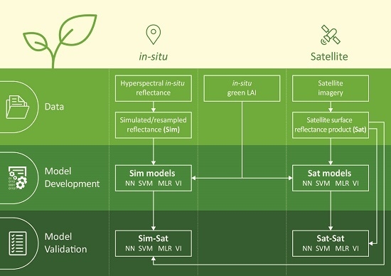
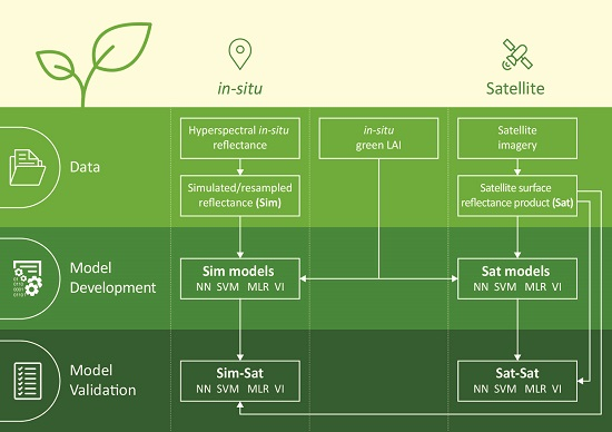
The work flow of the data and analyses is shown in Figure 1. Two spectral datasets were used: (a) hyperspectral reflectance, taken at close range, resampled to simulate spectral bands of sensors (denoted by Sim); and (b) surface reflectance satellite products (denoted by Sat). In accord with the datasets used, two types of models were developed for each technique: trained by simulated data (denoted by Sim) and trained by satellite data (denoted by Sat). Thus, for each technique two models of LAI estimation were developed:
- Sim-Sat—models trained by simulated data and validated by satellite data.
- Sat-Sat—models trained and validated by satellite data.
For estimating LAI by the recently launched MSI Sentinel 2 and OLCI Sentinel 3, hyperspectral reflectances taken at close range and resampled to simulate spectral bands of sensors were used for calibration and validation.
The training process was similar for all four techniques: first a band combination was chosen (during the study all the possible band combinations were tested). The dataset was subdivided into 10 random groups. Each band combination was tested 10 times using 10-fold cross- validation: each time a different combination of 90% of the dataset (nine sub-groups) was used for training and the unused 10% (one sub-group) formed the validation set. The newly-developed model, trained and validated using the simulated data, was then used to estimate LAI from the satellite data.
Normalized root mean square error (NRMSE) was used as an error metric:
where Meas denotes the measured green LAI, Pred denotes the predicted green LAI, and n is the number of measurements.
Each technique was trained using all of the possible band combinations. The number of bands used for training the non-parametric techniques varied from a single band up to the full set of bands in each satellite.
The uninformative variable elimination by partial least squares (UVE-PLS) method was used to identify informative spectral bands of TM/ETM+, MERIS and Sentinel 2. Each spectral band has a reliability value calculated on the basis of its regression coefficient in the model. The uninformative bands are the ones with a lower absolute reliability coefficient [21,44,45,46]. The reliability parameter is obtained by dividing the mean regression coefficient () by the standard deviation of the regression coefficient vector ():
3. Results and Discussion
3.1. Techniques and Analysis
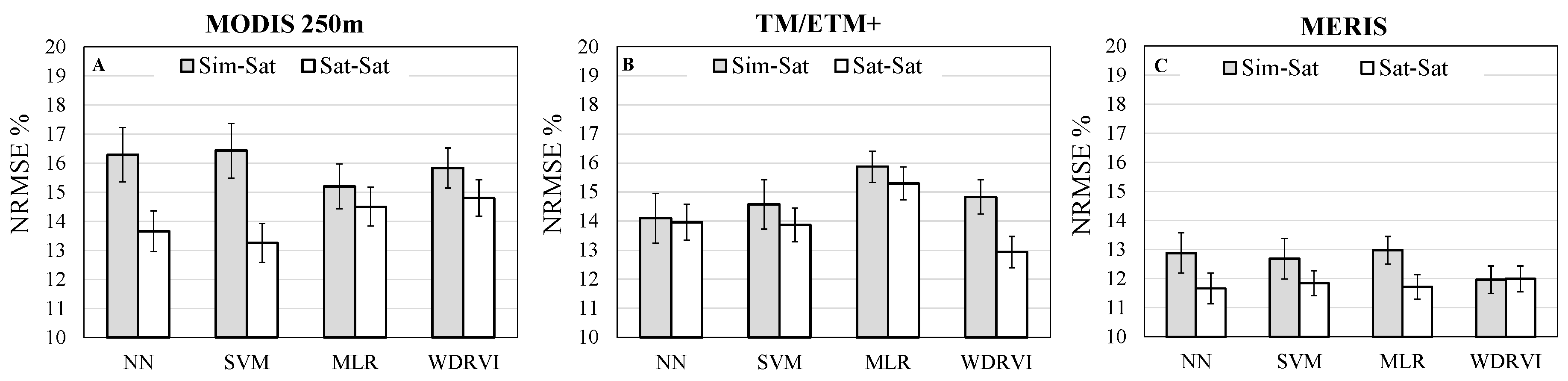
The accuracies of LAI estimation in both crops, maize and soybean, combined by models trained by simulated data and validated by satellite data (Sim-Sat), as well as trained and validated by satellite data (Sat-Sat), are presented in Figure 2 for each technique (NN, SVM, MLR, and VI) and each sensor. Among the VIs tested, WDRVI (α = 0.1) with NIR and either red (MODIS), green (Landsat), or red edge (MERIS) bands was the most accurate for all three sensors.
For MODIS 250 m resolution with two bands available, red and NIR, the models trained with satellite data (Sat-Sat) had NRMSE below 15% for all the techniques (Figure 2A). SVM and NN had the lowest NRMSE (below 13.5%).
Landsat data allowed for more accurate LAI estimation. Sat-Sat model using the SVM technique was able to estimate LAI with NRMSE below 14%. Sat-Sat model with WDRVI (NIR and green bands) had the lowest NRMSE (<13%).
The highest spectral resolution of the satellite data examined came from MERIS. The NRMSE of the Sim-Sat and Sat-Sat models was substantially lower than those that used MODIS and Landsat data. The estimation error of the Sim-Sat model was below 13% while that of the Sat-Sat model was below 12%. The lowest NRMSE, less than 11.6%, was achieved by the NN technique followed closely by the MLR, SVM, and WDRVI (with NIR and red edge spectral bands). The fact that vegetation indices are not significantly outperformed by NN, MLR, and SVM indicates that the NIR and red edge spectral bands contain most of the information necessary to estimate LAI in these crops.
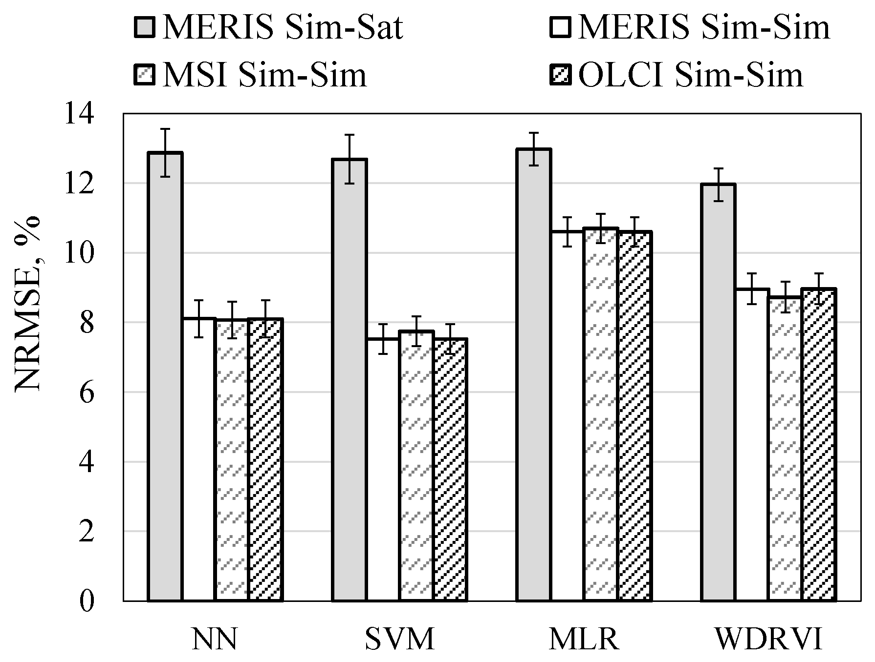
The use of multiyear MERIS data for LAI estimation is instructive for assessment of expected uncertainties of the recently launched OLCI Sentinel 3, which has band positions identical to MERIS, as well as MSI Sentinel 2, which has bands quite similar to MERIS. The NRMSE of the model trained and validated by data resampled to simulate reflectance in spectral bands of MERIS, MSI, and OLCI (denoted by Sim-Sim) were calculated and compared with NRMSE of the Sim-Sat MERIS model that was trained by simulated data and validated by MERIS surface reflectance products (Figure 3). NRMSE of the Sim-Sat MERIS model was around 12.5% while NRMSE of the Sim-Sim MERIS model, when NN and SVM techniques were used, was significantly lower—around 8% (Figure 2 and Figure 3). Thus, it is likely that the accuracy of LAI estimation by MSI Sentinel 2 and OLCI Sentinel 3 would be near the NRMSE found for MERIS Sim-Sat (below 13%) and Sat-Sat (below 12%) models (Figure 2C). However, the sample size of simulated data was much higher than satellite data and future studies are needed to confirm this conclusion.
MODIS and TM/ETM+ estimates of green LAI for the two crops taken together were less accurate than that of MERIS (Figure 2) due to differences in slopes of the relationships between the selected VI and green LAI for maize and soybean (Figure 4 for WDRVI; the same was the case for other techniques used—not shown). The MERIS red edge WDRVI was an accurate proxy of LAI: red edge WDRVI vs. LAI relationships were not statistically different for maize and soybean at the 0.05 probability level (p = 0.22, Figure 4B). This was not the case for MODIS; the relationships were significantly different (p < 0.008, Figure 4A) and, thus, species-specific. However, the use of MODIS and TM/ETM+ data allowed accurate assessment of green LAI in each crop separately (Table 2), confirming the results of MODIS LAI estimates in maize [32,47].
Sim-Sat validation demonstrated the accuracy of the Sim model (developed using close range data, Figure 1) for estimating LAI from satellite data. The Sim-Sat validation answered the question of whether models developed using multiyear close range observations could be used for retrieval of LAI from satellite data without re-parameterization. The results showed that the Sat model generally yielded about 1% more accurate estimation than the Sim model. However, the accuracy of the Sim model based on the use of vegetation indices with red edge bands (as in MERIS) was the same as that of the Sat model (Figure 2C). If these results would be confirmed using real Sentinel-2 and Sentinel-3 data, it will allow for the use of a model based on close range data for retrieval LAI from MSI and OLCI data.
3.2. Optimal Spectral Sampling
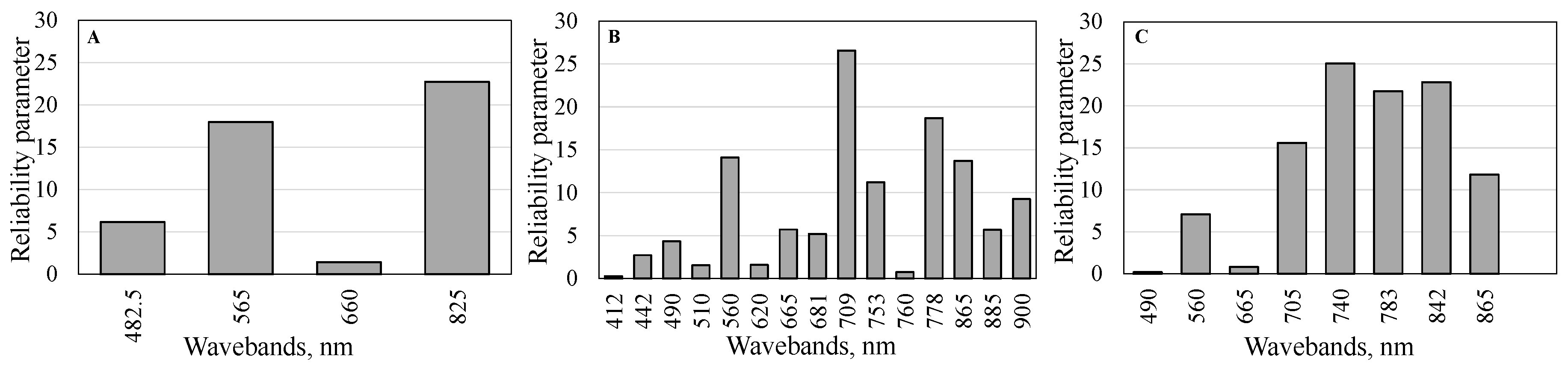
The information content of satellite data was assessed using the UVE-PLS reliability parameter: a small absolute value of the reliability parameter indicates that the reflectance in this band is less informative. Thus, uninformative or redundant spectral bands were identified for TM/ETM, MERIS, and MSI. The main spectral features of the reliability parameters of all sensors were (a) small values in the blue and red spectral regions; and (b) distinct peaks in the green, red edge, and NIR regions. Low-reliability parameter values in the blue and the red are due to the strong saturation of reflectance for LAI exceeding 2 and, thus, a decrease in the accuracy of the LAI estimation. The peaks in the green, red edge, and NIR indicate that bands located in these spectral regions are more useful for estimating LAI in the two crops taken together (Figure 5). The same features were found and discussed for the reliability parameter spectrum of hyperspectral data taken at close range in Kira et al. [21].
The next step was the identification of the spectral bands retained by the different techniques (NN, SVM, MLR, and VI). MODIS 250 m data contain reflectances in only two bands, while TM/ETM+ provided more possibilities for band selection. When only two spectral bands were allowed in the model, all techniques selected green and NIR bands. Among the non-parametric regression techniques, NN and SVM were the best—NRMSE of LAI estimation by both models, Sim-Sat and Sat-Sat, was around 14.4%. The addition of a third band (in the blue region) only slightly decreased the NRMSE (to 14%). When four bands were used (the fourth band was in the red region), NRMSE increased (Figure 6) likely due to overfitting at the training stage.
Thus, for NN and SVM, three bands—red edge, NIR, and blue—were retained for green LAI estimation in the two crops combined by TM/ETM+. The WDRVI with two bands, green and NIR, was able to estimate the green LAI with the NRMSE below 13% (Figure 2B). Importantly, all four techniques, NN, SVM, MLR, and WDRVI, selected the green and NIR bands. The selection of the NIR band was not surprising: multiple scattering inside leaves and between leaves in the canopy is the governing factor of reflectance in this spectral region, as documented in pioneering studies (e.g., [48]). The green range of the spectrum was found to be more sensitive to moderate to high LAI due to the much lower absorption coefficient of chlorophyll in the green than in the red region which prevents saturation of reflectance and provides deeper light penetration inside the leaves and canopy (e.g., [49,50,51,52,53]). The increase in accuracy when a third, blue, band was added may be explained by the high and similar (in both crops) sensitivity of blue reflectance to green LAI below 3 [21].
MERIS data has the highest spectral resolution of the satellite sensors examined; thus, it has the widest set of possible spectral bands. The Sim-Sat model with MLR and SVM techniques allowed LAI estimation with NRMSE below 13%. When the Sat-Sat model was used, the minimum NRMSE was below 11.8% for all three techniques, MLR, SVM, and NN (Figure 7). To achieve this accuracy, SVM used only two or three bands, and the addition of a fourth band decreased the accuracy. In contrast, MLR reached maximal accuracy using five bands, and NN, six bands. However, when the fifth and sixth bands were added the decrease in the NRMSE was very small (0.1%–0.25%). WDRVI with two bands, red edge and NIR, was able to achieve a NRMSE = 12% and explained more than 83% of LAI variation in the two crops taken together (Figure 2C and Figure 4B).
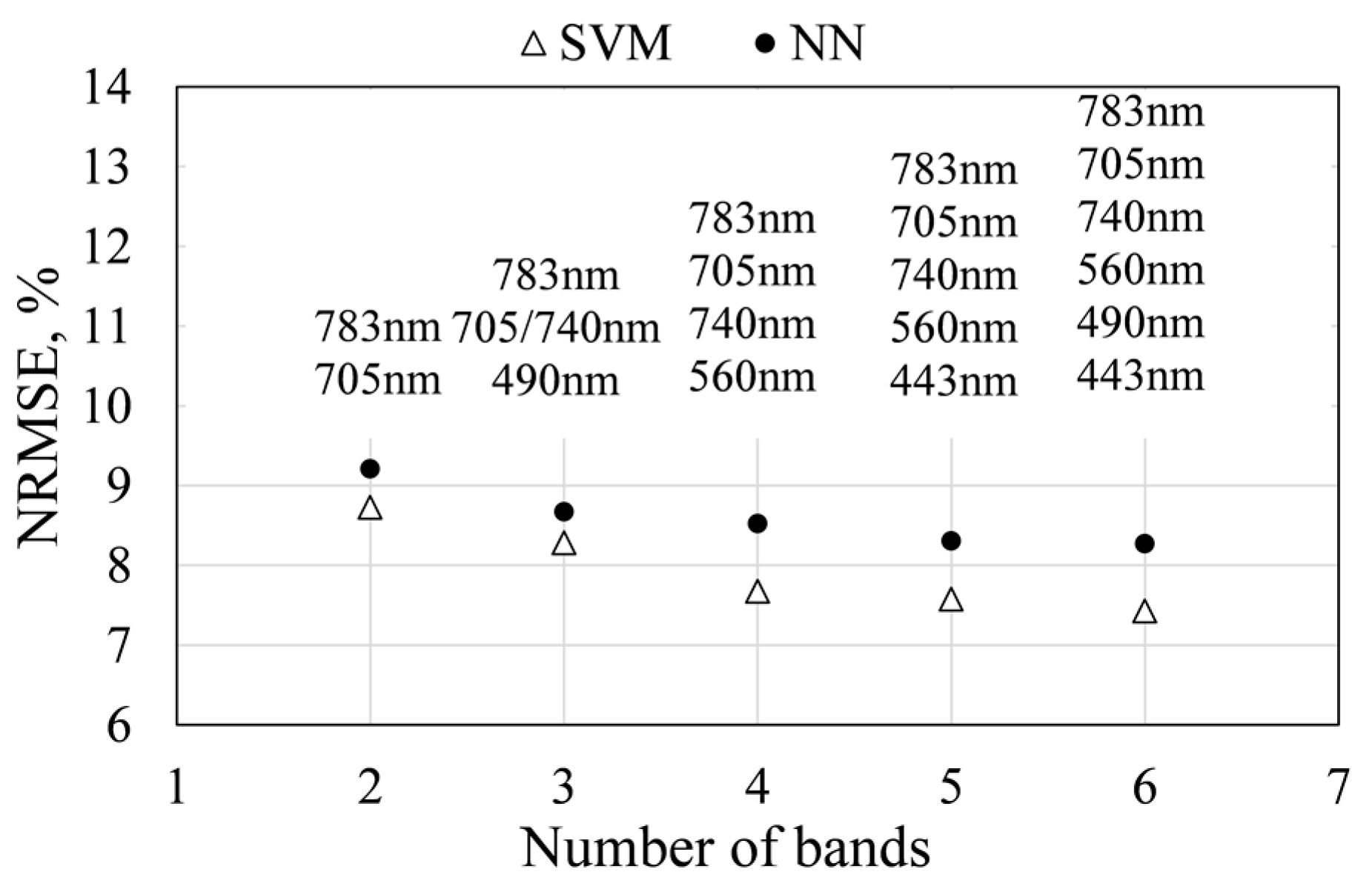
For MSI, the NIR and red edge band centered at 705 nm were retained in all techniques (SVM, NN, and MLR) when only two bands were allowed in the model (Figure 8). When three bands were used, the retained bands were red edge (either 705 or 740 nm), NIR, and blue. The addition of a fourth band, either the green or red edge at 740 nm, allowed for only slight decreases of the NRMSE from 8.5 to 8.3% for the NN and from 7.7% to 7.4% for the SVM. As in MERIS, the use of red edge and NIR bands was mandatory for accurate green LAI estimation.
Thus, three or four bands were sufficient to minimize the NRMSE of LAI estimation using satellite data by both Sim and Sat models. However, several studies have shown that increasing the number of bands above three or four did decrease the NRMSE of models trained and validated by simulated or aircraft data—seven spectral bands were needed to achieve the minimal error by NN using aircraft data [54], four to six (NN) and five to six (look up tables) band combinations using simulated data and data taken at close range [12], and six bands were selected by NN from nine synthetic bands [55]. Richter et al. [12] noted that while the results of selection analyses may depend on the algorithms employed, generally, the optimal number of bands for estimation of LAI is around six to eight. Moreover, they showed that the worst results were achieved through look up tables in combination with a two-band arrangement. This is in contrast to results of the present study showing that the two bands used by WDRVI were sufficient, achieving a NRMSE below 13% and 12% when TM/ETM+ and MERIS satellite data were used, respectively.
This is an important point for future studies; our results showed that when models trained either by simulated or satellite data were applied to satellite data (which is noisier than reflectance taken at close range), increasing the number of bands beyond three or four did not substantially improve estimation accuracy. An important implication, if this observation is confirmed in future studies, is that the quality of the satellite surface reflectance product (as it was in MERIS) limits the accuracy of the NN and SVM models for predicting LAI and, thus, the full potential of the multispectral sensors cannot be exploited. Whether this is a consequence of uncertainties in atmospheric correction or angular effects requires further investigation. Conversely, it may also be an artifact caused by the limited number of samples used in this study for MERIS (75 images, Table 1). More study is needed to see how far this finding can be pushed; i.e., whether or not it is apparent over other crops or in other locations.
Despite differing opinions concerning the importance of the red edge spectral region for LAI estimation [56,57] our results, based on satellite data, suggest that the use of the red edge range is crucial for obtaining the highest accuracies for LAI retrieval and its influence is more important than visible bands. The selection of spectral bands by all techniques was consistent with spectral band selection for foliar chlorophyll estimation performed by PROSPECT-5 ([58]). It is also consistent with the results of Feilhauer et al. [59] using a multi-method ensemble that provides a robust selection of spectral bands related to biochemical traits obtained for foliar chlorophyll content retrieval. Richter et al. [12,20] showed, using simulated data taken at close range, that MSI NIR and red edge spectral bands provided the most relevant information for LAI estimates. Weiss et al. [55], Bacour et al. [19], and Baret and Buis [2] came to the same conclusion.
Further, the present band selection is in accord with results from many earlier studies (e.g., [49,50,51,52]), observed that the reflectance in the region adjacent to the red chlorophyll absorption band (around 670 nm) becomes insensitive at moderate-to-high chlorophyll content (closely related to the green LAI) and the green range should be used for high-density vegetation [49,50,52]. The present results also support previous findings that the reflectance in the red edge region is strongly related to foliar and canopy chlorophyll content (e.g., [50,57,60,61,62,63,64,65]).
4. Conclusions
Models for accurate green LAI estimation using MODIS, Landsat, and MERIS data in two contrasting crops, maize and soybean, not requiring separate parameterization for each species, were developed. Multiple techniques, NN, SVM, MLR, and VI, were used to identify optimal spectral bands using either hyperspectral data taken at close range and resampled to spectral bands of satellite sensors or surface reflectance satellite products.
The selection of spectral bands agreed well with known absorption features of crops in a wide range of LAI variation. The band selection was consistent across the techniques used (NN, SVM, MLR) and the first two bands selected for each technique coincided with bands selected for vegetation indices. The agreement of different techniques to select a robust set of spectral bands related to green LAI, depending on the foliar trait (pigment content and composition) and structural trait (leaf area), is notable. The models applied to MERIS data consistently selected bands from the NIR and the red edge regions. When red edge bands were not available (as in Landsat TM/ETM+), the bands in the NIR and the green regions were selected. Across the multiyear datasets tested, each of the wavebands in these regions was selected consistently for each crop, maize and soybean, and in both crops combined.
The results of this study show that a multi-technique test provides a robust and consistent selection of spectral bands related to LAI estimation. Accurate satellite estimation of LAI across two contrasting crops was achieved by the MERIS with NRMSE below 12%. Hence, the spectral bands of MSI and OLCI bring valid information for LAI estimation. However, the retrieval accuracy of 10% for LAI targeted for the Sentinel 2 mission [66] was not achieved. For crops with photosynthetic stems, the inclusion of additional canopy components may improve accuracy towards reaching this goal.
A significant feature of this study is that the training and validation of the models was performed for different crops through a complete seasonal lifecycle (i.e., over the entire growing season). The results represent real crops with known pigment content, composition, green LAI, and their vertical distributions inside the canopy. The data may be used as a case study for comparison with radiative transfer model simulations of canopy reflectance in contrasting crops. To the best of our knowledge, the present study is one of the first where different models were trained by data taken during ten growing seasons in maize and soybean of different varieties under irrigated and rainfed conditions, different soil backgrounds (till vs. no till), and rotation of crops vs. continuous planting. Given that these crops have different photosynthetic pathways (C3 vs. C4), leaf structures (dicot vs. monocot) and canopy architectures (a heliotropic leaf angle distribution vs. a spherical leaf angle distribution), they cover a large spectrum of biophysical conditions. It would be of great interest for a further study to compare LAI estimation by the models presented here and by, e.g., a NN model based on data simulated by radiative transfer models (e.g., [12,19]). Such a study would give important insights into the realism of the pigmentation, leaf reflectance, and canopy structural properties that are assumed by such radiative transfer models.
Acknowledgments
This research was supported by NASA NACP and, partially, by the U.S. Department of Energy. We sincerely appreciate the support and the use of facilities and equipment provided by the Center for Advanced Land Management Information Technologies in the School of Natural Resources at the University of Nebraska-Lincoln. The US-Ne1, US-Ne2 and US-Ne3 AmeriFlux sites are supported by the Lawrence Berkeley National Lab AmeriFlux Data Management Program and by the Carbon Sequestration Program, University of Nebraska-Lincoln Agricultural Research Division. Funding for AmeriFlux core site data was provided by the U.S. Department of Energy’s Office of Science. AG is thankful to BARD and Marie Curie International Incoming Fellowships for supporting this study. We thank Toshihiro Sakamoto and Yi Peng for their assistance in processing the MODIS and Landsat TM/ETM+ data. We are grateful to Jose Moreno for providing the spectral response curves for MERIS and the sensors aboard the upcoming Sentinel satellites.
Author Contributions
O.K. and A.G. conceived of the project. A.N.-R., T.A., and A.G. collected or provided in situ reflectance and LAI data. A.N.-R. provided and analyzed satellite data. O.K., R.L., and A.G. performed data analysis. O.K. and A.G. drafted the manuscript. All authors contributed to discussion and preparation of the manuscript.
Conflicts of Interest
The authors declare no conflicts of interest.
References
- Cowling, S.A. Environmental control of leaf area production: Implications for vegetation and land-surface modeling. Glob. Biogeochem. Cycles 2003, 17, 1–14. [Google Scholar] [CrossRef]
- Baret, F.; Buis, S. Estimating canopy characteristics from remote sensing observations: Review of methods and associated problems. In Advances in Land Remote Sensing; Liang, S., Ed.; Springer: Dordrecht, The Netherlands; New York, NY, USA, 2008; pp. 173–201. [Google Scholar]
- Baret, F.; Guyot, G. Potentials and limits of vegetation indexes for LAI and APAR assessment. Remote Sens. Environ. 1991, 35, 161–173. [Google Scholar] [CrossRef]
- Thenkabail, P.S.; Enclona, E.A.; Ashton, M.S.; Van Der Meer, B. Accuracy assessments of hyperspectral waveband performance for vegetation analysis applications. Remote Sens. Environ. 2004, 91, 354–376. [Google Scholar] [CrossRef]
- Atzberger, C.; Guérif, M.; Baret, F.; Werner, W. Comparative analysis of three chemometric techniques for the spectroradiometric assessment of canopy chlorophyll content in winter wheat. Comput. Electron. Agric. 2010, 73, 165–173. [Google Scholar] [CrossRef]
- Verrelst, J.; Camps-Valls, G.; Muñoz-Marí, J.; Rivera, J.P.; Veroustraete, F.; Clevers, J.G.P.W.; Moreno, J. Optical remote sensing and the retrieval of terrestrial vegetation bio-geophysical properties—A review. ISPRS J. Photogramm. Remote Sens. 2015, 108, 273–290. [Google Scholar] [CrossRef]
- Atkinson, P.M.; Tatnall, A.R.L. Introduction Neural networks in remote sensing. Int. J. Remote Sens. 1997, 18, 699–709. [Google Scholar] [CrossRef]
- Verrelst, J.; Alonso, L.; Camps-Valls, G.; Delegido, J.; Moreno, J. Retrieval of vegetation biophysical parameters using Gaussian process techniques. Geosci. Remote Sens. IEEE Trans. 2012, 50, 1832–1843. [Google Scholar] [CrossRef]
- Baret, F.; Hagolle, O.; Geiger, B.; Bicheron, P.; Miras, B.; Huc, M.; Berthelot, B.; Niño, F.; Weiss, M.; Samain, O.; et al. LAI, fAPAR, and fCover CYCLOPES global products derived from VEGETATION Part 1: Principles of the algorithm. Remote Sens. Environ. 2007, 110, 275–286. [Google Scholar] [CrossRef]
- Jacquemoud, S.; Baret, F.; Andrieu, B.; Danson, F.M.; Jaggard, K. Extraction of vegetation biophysical parameters by inversion of the PROSPECT + SAIL models on sugar beet canopy reflectance data. Application to TM and AVIRIS sensors. Remote Sens. Environ. 1995, 52, 163–172. [Google Scholar] [CrossRef]
- Koetz, B.; Baret, F.; Poilvé, H.; Hill, J. Use of coupled canopy structure dynamic and radiative transfer models to estimate biophysical canopy characteristics. Remote Sens. Environ. 2005, 95, 115–124. [Google Scholar] [CrossRef]
- Richter, K.; Hank, T.B.; Vuolo, F.; Mauser, W.; D’Urso, G. Optimal exploitation of the sentinel-2 spectral capabilities for crop leaf area index mapping. Remote Sens. 2012, 4, 561–582. [Google Scholar] [CrossRef]
- Fava, F.; Colombo, R.; Bocchi, S.; Meroni, M.; Sitzia, M.; Fois, N.; Zucca, C. Identification of hyperspectral vegetation indices for Mediterranean pasture characterization. Int. J. Appl. Earth Obs. Geoinf. 2009, 11, 233–243. [Google Scholar] [CrossRef]
- Hansen, P.M.; Schjoerring, J.K. Reflectance measurement of canopy biomass and nitrogen status in wheat crops using normalized difference vegetation indices and partial least squares regression. Remote Sens. Environ. 2003, 86, 542–553. [Google Scholar] [CrossRef]
- Haboudane, D.; Miller, J.R.; Pattey, E.; Zarco-Tejada, P.J.; Strachan, I.B. Hyperspectral vegetation indices and novel algorithms for predicting green LAI of crop canopies: Modeling and validation in the context of precision agriculture. Remote Sens. Environ. 2004, 90, 337–352. [Google Scholar] [CrossRef]
- Viña, A.; Gitelson, A.A.; Nguy-Robertson, A.L.; Peng, Y. Comparison of different vegetation indices for the remote assessment of green leaf area index of crops. Remote Sens. Environ. 2011, 115, 3468–3478. [Google Scholar] [CrossRef]
- Nguy-Robertson, A.L.; Peng, Y.; Gitelson, A.A.; Arkebauer, T.J.; Pimstein, A.; Herrmann, I.; Karnieli, A.; Rundquist, D.C.; Bonfil, D.J. Estimating green LAI in four crops: Potential of determining optimal spectral bands for a universal algorithm. Agric. For. Meteorol. 2014, 192–193, 140–148. [Google Scholar] [CrossRef]
- Verrelst, J.; Muñoz, J.; Alonso, L.; Delegido, J.; Rivera, J.P.; Camps-Valls, G.; Moreno, J. Machine learning regression algorithms for biophysical parameter retrieval: Opportunities for Sentinel-2 and -3. Remote Sens. Environ. 2012, 118, 127–139. [Google Scholar] [CrossRef]
- Bacour, C.; Baret, F.; Béal, D.; Weiss, M.; Pavageau, K. Neural network estimation of LAI, fAPAR, fCover and LAI×Cab, from top of canopy MERIS reflectance data: Principles and validation. Remote Sens. Environ. 2006, 105, 313–325. [Google Scholar] [CrossRef]
- Richter, K.; Atzberger, C.; Vuolo, F.; Weihs, P.; D’Urso, G. Experimental assessment of the Sentinel-2 band setting for RTM-based LAI retrieval of sugar beet and maize. Can. J. Remote Sens. 2009, 35, 230–247. [Google Scholar] [CrossRef]
- Kira, O.; Nguy-Robertson, A.L.; Arkebauer, T.J.; Linker, R.; Gitelson, A.A. Informative spectral bands for remote green LAI estimation in C3 and C4 crops. Agric. For. Meteorol. 2016, 218–219, 243–249. [Google Scholar] [CrossRef]
- Verma, S.B.; Dobermann, A.; Cassman, K.G.; Walters, D.T.; Knops, J.M.; Arkebauer, T.J.; Suyker, A.E.; Burba, G.G.; Amos, B.; Yang, H.; et al. Annual carbon dioxide exchange in irrigated and rainfed maize-based agroecosystems. Agric. For. Meteorol. 2005, 131, 77–96. [Google Scholar] [CrossRef]
- Suyker, A.E.; Verma, S.B. Gross primary production and ecosystem respiration of irrigated and rainfed maize-soybean cropping systems over 8 years. Agric. For. Meteorol. 2012, 165, 12–24. [Google Scholar] [CrossRef]
- Breda, N.J.J. Ground-based measurements of leaf area index: A review of methods, instruments and current controversies. J. Exp. Bot. 2003, 54, 2403–2417. [Google Scholar] [CrossRef] [PubMed]
- Nguy-Robertson, A.; Peng, Y.; Arkebauer, T.; Scoby, D.; Schepers, J.; Gitelson, A. Communications in Soil Science and Plant Analysis Using a Simple Leaf Color Chart to Estimate Leaf and Canopy Chlorophyll a Content in Maize (Zea mays). Commun. Soil Sci. Plant Anal. 2015, 46, 2734–2745. [Google Scholar] [CrossRef]
- Peng, Y.; Nguy-Robertson, A.; Arkebauer, T.; Gitelson, A.A. Assessment of Canopy Chlorophyll Content Retrieval in Maize and Soybean: Implications of Hysteresis on the Development of Generic Algorithms. Remote Sens. 2017, 9, 226. [Google Scholar] [CrossRef]
- Law, B.E.; Arkebauer, T.; Campbell, J.L.; Chen, J.; Sun, O.; Schwartz, M.; van Ingen, C.; Verma, S. Terrestrial Carbon Observations: Protocols for Vegetation Sampling and Data Submission; Report of the Global Terrestrial Observing System (GTOS); Food and Agriculture Organization of United Nation (FAO): Rome, Italy, 2008. [Google Scholar]
- Nguy-Robertson, A.; Gitelson, A.; Peng, Y.; Viña, A.; Arkebauer, T.; Rundquist, D. Green leaf area index estimation in maize and soybean: Combining vegetation indices to achieve maximal sensitivity. Agron. J. 2012, 104, 1336–1347. [Google Scholar] [CrossRef]
- Rundquist, D.; Perk, R.; Leavitt, B.; Keydan, G.; Gitelson, A. Collecting spectral data over cropland vegetation using machine-positioning versus hand-positioning of the sensor. Comput. Electron. Agric. 2004, 43, 173–178. [Google Scholar] [CrossRef]
- Rundquist, D.; Gitelson, A.; Leavitt, B.; Zygielbaum, A.; Perk, R.; Keydan, G. Elements of an Integrated Phenotyping System for Monitoring Crop Status at Canopy Level. Agronomy 2014, 4, 108–123. [Google Scholar] [CrossRef]
- Huete, A.; Didan, K.; Miura, T.; Rodriguez, E.P.; Gao, X.; Ferreira, L.G. Overview of the radiometric and biophysical performance of the MODIS vegetation indices. Remote Sens. Environ. 2002, 83, 195–213. [Google Scholar] [CrossRef]
- Guindin-Garcia, N.; Gitelson, A.A.; Arkebauer, T.J.; Shanahan, J.; Weiss, A. An evaluation of MODIS 8- and 16-day composite products for monitoring maize green leaf area index. Agric. For. Meteorol. 2012, 161, 15–25. [Google Scholar] [CrossRef]
- Sakamoto, T.; Gitelson, A.A.; Nguy-Robertson, A.L.; Arkebauer, T.J.; Wardlow, B.D.; Suyker, A.E.; Verma, S.B.; Shibayama, M. An alternative method using digital cameras for continuous monitoring of crop status. Agric. For. Meteorol. 2012, 154–155, 113–126. [Google Scholar] [CrossRef]
- Masek, J.G.; Vermote, E.F.; Saleous, N.E.; Wolfe, R.; Hall, F.G.; Huemmrich, K.F.; Gao, F.; Kutler, J.; Lim, T.K. A landsat surface reflectance dataset for North America, 1990–2000. IEEE Geosci. Remote Sens. Lett. 2006, 3, 68–72. [Google Scholar] [CrossRef]
- Gitelson, A.A.; Peng, Y.; Masek, J.G.; Rundquist, D.C.; Verma, S.; Suyker, A.; Baker, J.M.; Hatfield, J.L.; Meyers, T. Remote estimation of crop gross primary production with Landsat data. Remote Sens. Environ. 2012, 121, 404–414. [Google Scholar] [CrossRef]
- Guanter, L.; Del Carmen González-Sanpedro, M.; Moreno, J. A method for the atmospheric correction of ENVISAT/MERIS data over land targets. Int. J. Remote Sens. 2007, 28, 709–728. [Google Scholar] [CrossRef]
- Abuelgasim, A.A.; Gopal, S.; Strahler, A.H. Forward and inverse modelling of canopy directional reflectance using a neural network. Int. J. Remote Sens. 1998, 19, 453–471. [Google Scholar] [CrossRef]
- Duveiller, G.; Weiss, M.; Baret, F.; Defourny, P. Retrieving wheat Green Area Index during the growing season from optical time series measurements based on neural network radiative transfer inversion. Remote Sens. Environ. 2011, 115, 887–896. [Google Scholar] [CrossRef]
- Smith, J.A.H. LAI inversion using a back-propagation neural network trained with a multiple scattering model. IEEE Trans. Geosci. Remote Sens. 1993, 31, 1102–1106. [Google Scholar] [CrossRef]
- Weiss, M.; Baret, F. Evaluation of canopy biophysical variable retrieval performances from the accumulation of large swath satellite data. Remote Sens. Environ. 1999, 70, 293–306. [Google Scholar] [CrossRef]
- Vapnick, V.N. Statistical Learning Theory; Wiley: New York, NY, USA, 1998. [Google Scholar]
- Camps-Valls, G.; Bruzzone, L.; Rojo-Álvarez, J.L.; Melgani, F. Robust support vector regression for biophysical variable estimation from remotely sensed images. IEEE Geosci. Remote Sens. Lett. 2006, 3, 339–343. [Google Scholar] [CrossRef]
- Gitelson, A.A. Wide Dynamic Range Vegetation Index for remote quantification of biophysical characteristics of vegetation. J. Plant Physiol. 2004, 161, 165–173. [Google Scholar] [CrossRef] [PubMed]
- Cai, W.; Li, Y.; Shao, X. A variable selection method based on uninformative variable elimination for multivariate calibration of near-infrared spectra. Chemom. Intell. Lab. Syst. 2008, 90, 188–194. [Google Scholar] [CrossRef]
- Centner, V.; Massart, D.L.; de Noord, O.E.; de Jong, S.; Vandeginste, B.M.; Sterna, C. Elimination of uninformative variables for multivariate calibration. Anal. Chem. 1996, 68, 3851–3858. [Google Scholar] [CrossRef] [PubMed]
- Kira, O.; Linker, R.; Gitelson, A. Non-destructive estimation of foliar chlorophyll and carotenoid contents: Focus on informative spectral bands. Int. J. Appl. Earth Obs. Geoinform. 2015, 38, 251–260. [Google Scholar] [CrossRef]
- Sakamoto, T.; Gitelson, A.A.; Arkebauer, T.J. MODIS-based corn grain yield estimation model incorporating crop phenology information. Remote Sens. Environ. 2013, 131, 215–231. [Google Scholar] [CrossRef]
- Gausman, H.W.; Allen, W.A.; Cardenas, R. Reflectance of cotton leaves and their structure. Remote Sens. Environ. 1969, 1, 19–22. [Google Scholar] [CrossRef]
- Buschmann, C.; Nagel, E. In vivo spectroscopy and internal optics of leaves as basis for remote sensing of vegetation. Int. J. Remote Sens. 1993, 14, 711–722. [Google Scholar] [CrossRef]
- Gitelson, A.; Merzlyak, M.N. Spectral Reflectance Changes Associated with Autumn Senescence of Aesculus-hippocastanum L. and Acer-platanoides L. Leaves—Spectral Features and Relation to Chlorophyll Estimation. J. Plant Physiol. 1994, 143, 286–292. [Google Scholar] [CrossRef]
- Geosci, T.; Sens, R.; Hall, F.G. The interpretation of spectral vegetation. IEEE Trans. Geosci. Remote Sens. 1995, 33, 481–486. [Google Scholar]
- Thomas, J.R.; Gausman, H.W. Leaf reflectance vs. leaf chlorophyll and carotenoid concentrations for eight crops. Agron. J. 1977, 69, 799. [Google Scholar] [CrossRef]
- Yoder, B.J.; Waring, R.H. The normalized difference vegetation index of small Douglas-fir canopies with varying chlorophyll concentrations. Remote Sens. Environ. 1994, 49, 81–91. [Google Scholar] [CrossRef]
- Verger, A.; Baret, F.; Camacho, F. Optimal modalities for radiative transfer-neural network estimation of canopy biophysical characteristics: Evaluation over an agricultural area with CHRIS/PROBA observations. Remote Sens. Environ. 2011, 115, 415–426. [Google Scholar] [CrossRef]
- Weiss, M.; Baret, F.; Myneni, R.B.; Pragnère, A.; Knyazikhin, Y. Investigation of a model inversion technique to estimate canopy biophysical variables from spectral and directional reflectance data. Agronomie 2000, 20, 3–22. [Google Scholar] [CrossRef]
- Darvishzadeh, R.; Atzberger, C.; Skidmore, A.K.; Abkar, A.A. Leaf Area Index derivation from hyperspectral vegetation indicesand the red edge position. Int. J. Remote Sens. 2009, 30, 6199–6218. [Google Scholar] [CrossRef]
- Delegido, J.; Verrelst, J.; Alonso, L.; Moreno, J. Evaluation of sentinel-2 red-edge bands for empirical estimation of green LAI and chlorophyll content. Sensors 2011, 11, 7063–7081. [Google Scholar] [CrossRef] [PubMed]
- Féret, J.-B.; François, C.; Gitelson, A.A.; Asner, G.P.; Barry, K.M.; Panigada, C.; Richardson, A.D.; Jacquemoud, S. Optimizing spectral indices and chemometric analysis of leaf chemical properties using radiative transfer modeling. Remote Sens. Environ. 2011, 115, 2742–2750. [Google Scholar] [CrossRef]
- Feilhauer, H.; Asner, G.P.; Martin, R.E. Multi-method ensemble selection of spectral bands related to leaf biochemistry. Remote Sens. Environ. 2015, 164, 57–65. [Google Scholar] [CrossRef]
- Aoki, M.; Yabuki, K.; Totsuka, T.; Nisrnda, M. Remote sensing of chlorophyll content of leaf (I) effective spectral reflection characteristics of leaf for the evaluation of chlorophyll content in leaves of dicotyledons. Control Biol. 1986, 24, 21–26. [Google Scholar] [CrossRef]
- Carter, G.A. Ratios of leaf reflectances in narrow wavebands as indicators of plant stress. Int. J. Remote Sens. 1994, 15, 697–703. [Google Scholar] [CrossRef]
- Curran, P.J.; Windham, W.R.; Gholz, H.L. Exploring the relationship between reflectance red edge and chlorophyll content in slash pine leaves. Tree Physiol. 1995, 3, 203–206. [Google Scholar] [CrossRef]
- Dash, J.; Curran, P.J. The MERIS terrestrial chlorophyll index. Int. J. Remote Sens. 2004, 2523, 5403–5413. [Google Scholar] [CrossRef]
- Gamon, J.A.; Surfus, J.S. Assessing leaf pigment content and activity with a reflectometer. New Phytol. 1999, 143, 105–117. [Google Scholar] [CrossRef]
- Gitelson, A.A.; Viña, A.; Ciganda, V.; Rundquist, D.C.; Arkebauer, T.J. Remote estimation of canopy chlorophyll content in crops. Geophys. Res. Lett. 2005, 32, 1–4. [Google Scholar] [CrossRef]
- Drusch, M.; Gascon, F.; Berger, M. GMES Sentinel-2: Mission requirements document. Earth 2010. [Google Scholar]
Figure 1.
Work flow of the data and analyses. Four techniques were employed: support vector machines (SVM), neural network (NN), multiple linear regression (MLR), and vegetation indices (VI). For each technique, two models were developed differing in terms of the data used for calibration: Sim models based on hyperspectral data resampled to simulate spectral bands of satellite sensors, and Sat models based on satellite surface reflectance products. Both models were validated using satellite data.
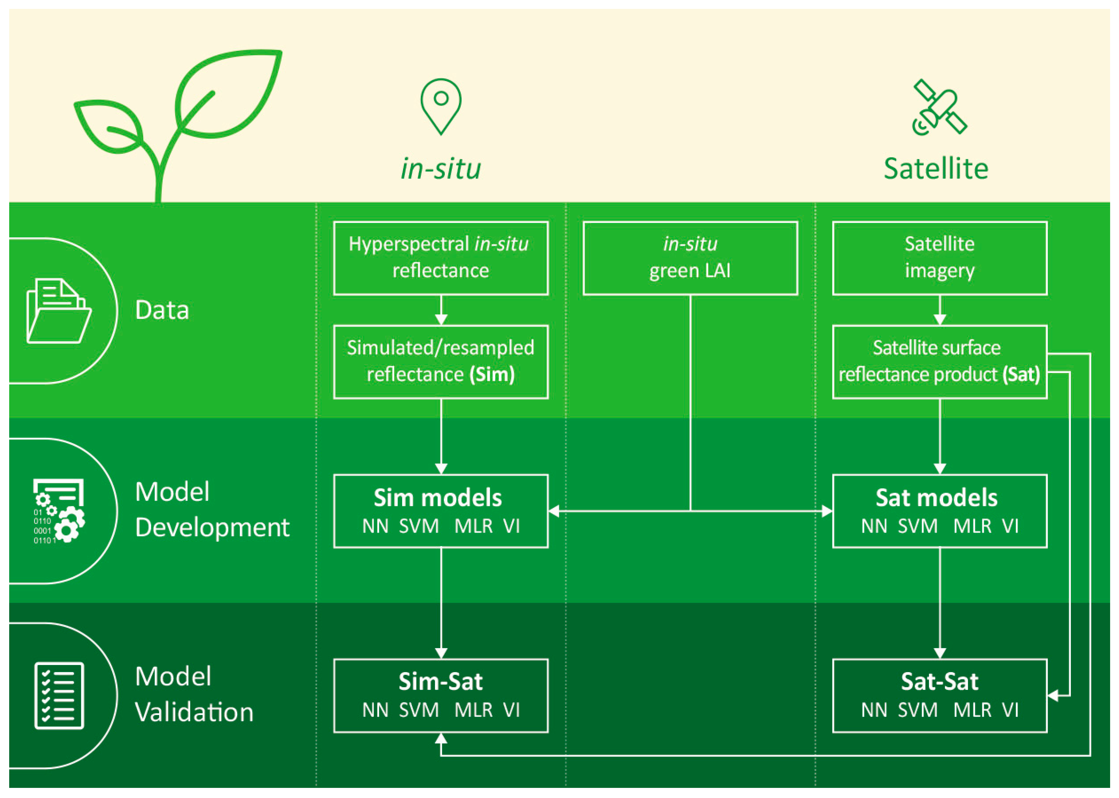
Figure 2.
Normalized root mean square errors of green LAI estimation in maize and soybean taken together and their standard deviations (bars) using four techniques (NN, SVM, MLR, and WDRVI) for three satellite sensors: (A) MODIS 250 m resolution; (B) TM/ETM+; and (C) MERIS. Sim-Sat models were trained by reflectance taken at close range resampled to simulate reflectance in spectral bands of satellite sensors and validated by satellite surface reflectance products; Sat-Sat—models were trained and validated by satellite surface reflectance products.

Figure 3.
NRMSE of green LAI estimation in both crops, maize and soybean, by models trained and validated by MERIS satellite products, MERIS Sim-Sat, and trained and validated by reflectance data taken at close range resampled to simulate reflectance in spectral bands of MERIS, MSI, and OLCI (MERIS Sim-Sim, MSI Sim-Sim and OLCI Sim-Sim, respectively).

Figure 4.
Relationships between (A) MODIS WDRVI and (B) MERIS WDRVI and green LAI in maize and soybean. WDRVI was calculated using MODIS (red and NIR) and MERIS (red edge and NIR) surface reflectance products. The number of points are summarized in Table 1.
Figure 4.
Relationships between (A) MODIS WDRVI and (B) MERIS WDRVI and green LAI in maize and soybean. WDRVI was calculated using MODIS (red and NIR) and MERIS (red edge and NIR) surface reflectance products. The number of points are summarized in Table 1.
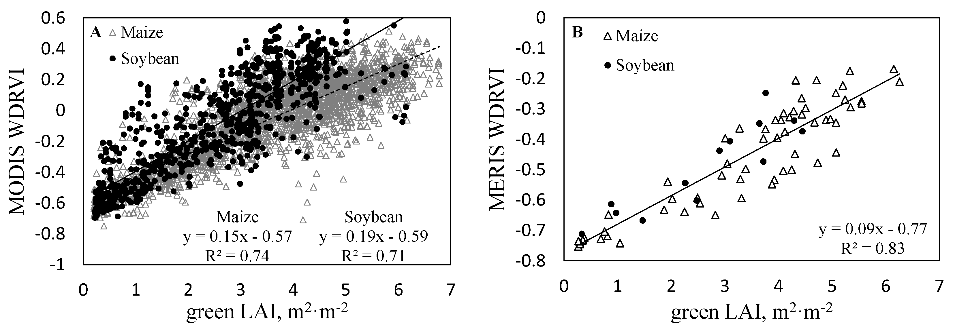
Figure 5.
Reliability parameters calculated using the uninformative variable elimination partial least squares technique for LAI estimation in maize and soybean combined plotted versus central wavelength of spectral bands of (A) TM/ETM+; (B) MERIS; and (C) MSI. Reliability parameters were calculated using TM/ETM+ and MERIS satellite data and simulated MSI data. For TM/ETM+ and MERIS surface reflectance satellite products were used and for MSI data taken at close range was resampled to MSI spectral bands.

Figure 6.
Normalized root mean square error (NRMSE) of green LAI estimation by NN with different numbers of TM/ETM+ spectral bands used. The NRMSE by SVM was virtually the same as NN. Wavelengths corresponding to the centers of the bands used are shown. Sim-Sat models were trained by reflectances taken at close range and resampled to simulate TM/ETM+ bands and validated by surface reflectance satellite products; Sat-Sat—trained and validated by surface reflectance satellite products.
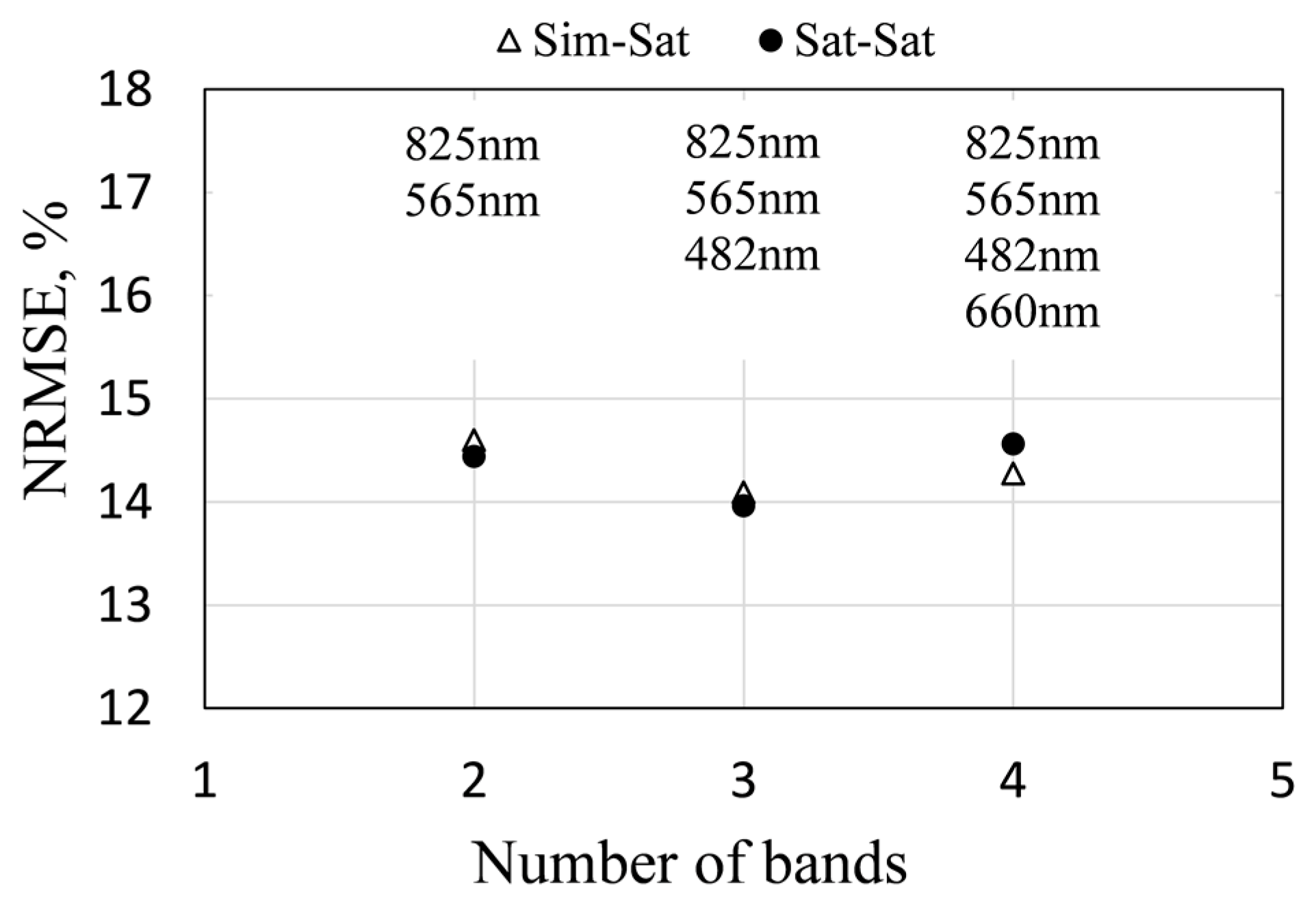
Figure 7.
NRMSE of green LAI estimation with different numbers of spectral bands used in MERIS data by (A) multiple linear regression (MLR); (B) neural network (NN); and (C) support vector machine (SVM) regression. Wavelengths corresponding to the centers of the bands used are shown. Each model was trained and validated by different data: Sim-Sat model was trained by data taken at close range, resampled to simulate spectral bands of MERIS and validated by MERIS surface reflectance products; Sat-Sat—trained and validated by MERIS surface reflectance products.
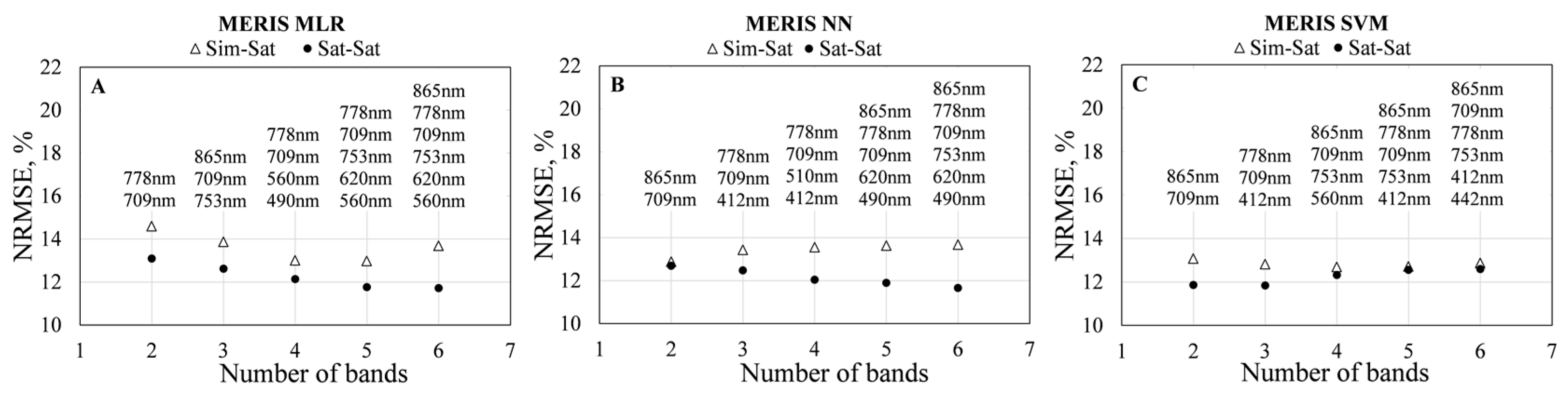
Figure 8.
NRMSE of green LAI estimation with different numbers of spectral bands used in MSI data by the support vector machines (SVM) and neural network (NN) techniques. Wavelengths corresponding to the centers of the bands used are shown. Each model for green LAI estimation was trained and validated by data taken at close range resampled to simulate the spectral bands of MSI.

Table 1.
Summary of sample size (n) and maximal green leaf area index (LAI) in m2·m−2 for in situ and satellite imagery data sets for both maize and soybean.
Table 1.
Summary of sample size (n) and maximal green leaf area index (LAI) in m2·m−2 for in situ and satellite imagery data sets for both maize and soybean.
| Sensor | Years Acquired | Crop | n | Maximum LAI |
|---|---|---|---|---|
| In situ | 2001–2008 | Maize | 266 | 6.48 |
| Soybean | 133 | 6.15 | ||
| MODIS | 2001–2012 | Maize | 2693 | 6.72 |
| Soybean | 906 | 6.08 | ||
| TM and ETM+ | 2001–2008 | Maize | 167 | 6.29 |
| Soybean | 44 | 5.73 | ||
| MERIS | 2003–2011 | Maize | 61 | 6.26 |
| Soybean | 14 | 4.45 |
Table 2.
Normalized root mean square errors (in percent) of LAI estimation in maize and soybean using four techniques (NN, SVM, MLR, and WDRVI) for two satellite sensors: MODIS 250 m resolution and TM/ETM+. Sim-Sat—models trained by reflectance taken at close range resampled to simulate reflectance in spectral bands of MODIS and TM/ETM+ and validated by satellite surface reflectance product; Sat-Sat—models trained and validated by satellite surface reflectance product. Red WDRVI was used for MODIS and green WDRVI for TM/ETM+.
| MODIS | TM/ETM+ | |||
|---|---|---|---|---|
| Sim-Sat | Sat-Sat | Sim-Sat | Sat-Sat | |
| Maize | ||||
| MLR | 12.12 | 12.03 | 13.04 | 11.79 |
| NN | 15.84 | 11.55 | 13.10 | 10.55 |
| SVM | 15.90 | 11.52 | 12.94 | 10.36 |
| WDRVI | 13.52 | 12.60 | 12.52 | 11.12 |
| Soybean | ||||
| MLR | 13.31 | 13.22 | 14.46 | 10.91 |
| NN | 14.57 | 13.01 | 10.49 | 10.81 |
| SVM | 14.24 | 13.10 | 10.52 | 11.33 |
| WDRVI | 13.44 | 13.20 | 12.39 | 11.55 |
© 2017 by the authors. Licensee MDPI, Basel, Switzerland. This article is an open access article distributed under the terms and conditions of the Creative Commons Attribution (CC BY) license (http://creativecommons.org/licenses/by/4.0/).
Share and Cite
MDPI and ACS Style
Kira, O.; Nguy-Robertson, A.L.; Arkebauer, T.J.; Linker, R.; Gitelson, A.A. Toward Generic Models for Green LAI Estimation in Maize and Soybean: Satellite Observations. Remote Sens. 2017, 9, 318. https://doi.org/10.3390/rs9040318
AMA Style
Kira O, Nguy-Robertson AL, Arkebauer TJ, Linker R, Gitelson AA. Toward Generic Models for Green LAI Estimation in Maize and Soybean: Satellite Observations. Remote Sensing. 2017; 9(4):318. https://doi.org/10.3390/rs9040318
Chicago/Turabian StyleKira, Oz, Anthony L. Nguy-Robertson, Timothy J. Arkebauer, Raphael Linker, and Anatoly A. Gitelson. 2017. "Toward Generic Models for Green LAI Estimation in Maize and Soybean: Satellite Observations" Remote Sensing 9, no. 4: 318. https://doi.org/10.3390/rs9040318
Note that from the first issue of 2016, this journal uses article numbers instead of page numbers. See further details here.