Article

Supervised and Semi-Supervised Multi-View Canonical Correlation Analysis Ensemble for Heterogeneous Domain Adaptation in Remote Sensing Image Classification

1
State Key Laboratory of Desert and Oasis Ecology, Xinjiang Institute of Ecology and Geography, Chinese Academy of Sciences, Urumqi 830011, China
2
CAS Research Center for Ecology and Environment of Central Asia, Chinese Academy of Sciences, Urumqi 830011, China
3
Department of Earth Observation Science, Faculty of Geo-Information Science and Earth Observation (ITC), University of Twente, 7500 AE Enschede, The Netherlands
4
Department of Electrical, Computer and Biomedical Engineering, University of Pavia, Pavia 27100, Italy
5
College of Surveying and Geoinformatics, Tongji University, Shanghai 200092, China
6
Department of Geographical Information Science, Nanjing University, Nanjing 210000, China
*
Author to whom correspondence should be addressed.
Remote Sens. 2017, 9(4), 337; https://doi.org/10.3390/rs9040337
Submission received: 7 January 2017 / Revised: 28 March 2017 / Accepted: 29 March 2017 / Published: 1 April 2017
(This article belongs to the Special Issue Learning to Understand Remote Sensing Images)

Abstract

:
In this paper, we present the supervised multi-view canonical correlation analysis ensemble (SMVCCAE) and its semi-supervised version (SSMVCCAE), which are novel techniques designed to address heterogeneous domain adaptation problems, i.e., situations in which the data to be processed and recognized are collected from different heterogeneous domains. Specifically, the multi-view canonical correlation analysis scheme is utilized to extract multiple correlation subspaces that are useful for joint representations for data association across domains. This scheme makes homogeneous domain adaption algorithms suitable for heterogeneous domain adaptation problems. Additionally, inspired by fusion methods such as Ensemble Learning (EL), this work proposes a weighted voting scheme based on canonical correlation coefficients to combine classification results in multiple correlation subspaces. Finally, the semi-supervised MVCCAE extends the original procedure by incorporating multiple speed-up spectral regression kernel discriminant analysis (SRKDA). To validate the performances of the proposed supervised procedure, a single-view canonical analysis (SVCCA) with the same base classifier (Random Forests) is used. Similarly, to evaluate the performance of the semi-supervised approach, a comparison is made with other techniques such as Logistic label propagation (LLP) and the Laplacian support vector machine (LapSVM). All of the approaches are tested on two real hyperspectral images, which are considered the target domain, with a classifier trained from synthetic low-dimensional multispectral images, which are considered the original source domain. The experimental results confirm that multi-view canonical correlation can overcome the limitations of SVCCA. Both of the proposed procedures outperform the ones used in the comparison with respect to not only the classification accuracy but also the computational efficiency. Moreover, this research shows that canonical correlation weighted voting (CCWV) is a valid option with respect to other ensemble schemes and that because of their ability to balance diversity and accuracy, canonical views extracted using partially joint random view generation are more effective than those obtained by exploiting disjoint random view generation.

Graphical Abstract

1. Introduction

Supervised learning algorithms predominate over all other land cover mapping/monitoring techniques that use remote sensing (RS) data. However, the performance of supervised learning algorithms varies as a function of labeled training data properties, such as the sample size and the statistically unbiased and discriminative capabilities of the features extracted from the data [1]. As monitoring requires multi-temporal images, radiometric differences, atmospheric and illumination conditions, seasonal variations, and variable acquisition geometries can affect supervised techniques, potentially causing a distribution shift in the training data [2,3]. Regardless of the cause, any distribution change or domain shift that occurs after learning a classifier can degrade performance.
In the pattern recognition (PR) and RS image classification communities, this challenge is commonly referred to as covariate shift [4] or sample selection bias [5]. Many solutions have been proposed to resolve this problem, including image-to-image normalization [6], absolute and relative image normalization [7,8], histogram matching [9], and a multivariate extension of the univariate matching [10]. Recently, domain adaptation (DA) techniques, which attempt to mitigate performance the degradation caused by a distribution shift, has attracted increasing attention and is widely considered to provide an efficient solution [11,12,13,14,15,16].
According to the technical literature in PR and machine learning (ML), DA is a special case of transductive transfer learning (TTL). Its goal is to learn a function that predicts the label of a novel test sample in the target domain [12,15]. Depending on the availability of the source and the target domain data, the DA problem can result into supervised domain adaptation (SDA), semi-supervised domain adaptation (SSDA), unsupervised domain adaptation (UDA), multisource domain adaptation (MSDA) and heterogeneous domain adaption (HDA) [14,15,16,17,18,19].
Moreover, according to the “knowledge” transferred across domains or tasks, classical approaches to DA can be grouped into parameter adapting, instance transferring, feature representation, and relational knowledge transfer techniques.
Parameter adapting approaches aim to transfer and adapt a classification model and/or its parameters to the target domain; the model and/or parameters are learned from the source domain (SD) [20]. The seminal work presented by Khosla et al. [5] and Woodcock et al. [7], which features parameter adjustment for a maximum-likelihood classifier in a multiple cascade classifier system by retraining, can be categorized into this group.
In instance transferring, the samples from the SD are reweighted [21] or resampled [22] for their use in the TD. In the RS community, active learning (AL) has also been applied to address DA problems. For example, AL for DA in the supervised classification RS images is proposed by Persello and Bruzzone [23] via iteratively labeling and adding to the training set the minimum number of the most informative samples from the target domain, while removing the source-domain samples that do not fit with the distributions of the classes in the TD.
For the third group, feature representation-based adaptation searches for a set of shared and invariant features using feature extraction (FE), feature selection (FS) or manifold alignment to reduce the marginal, conditional and joint distributions between the domains [16,24,25,26]. Matasci et al. [14] investigated the semi-supervised transfer component analysis (SSTCA) [27] for both hyperspectral and multispectral high resolution image classification, whereas Samat et al. [16] analyzed a geodesic Gaussian flow kernel based support vector machine (GFKSVM) in the context of hyperspectral image classification, which adopts several unsupervised linear and nonlinear subspace feature transfer techniques.
Finally, relational knowledge transfer techniques address the problem of how to leverage the knowledge acquired in SD to improve accuracy and learning speed in a related TD [28].
Among these four groups, it is easy to recognize the importance of RS image classification of adaptation strategies based on feature representation. However, most previous studies have assumed that data from different domains are represented by the same types of features with the same dimensions. Thus, these techniques cannot handle the problem of data from source and target domains represented by heterogeneous features with different dimensions [18,29]. One example of this scenario is land cover updating using current RS data; each time, there are different features with finer spatial resolution and more spectral bands (e.g., Landsat 8 OLI with nine spectral bands at 15–30 m spatial resolution, and Airborne Visible/Infrared Imaging Spectrometer (AVIRIS) with 224 spectral bands at 20 m spatial resolution), when the training data are only available at coarser spatial and spectral resolutions (e.g., MSS with four spectral bands and 60 m spatial resolution).
One of the simplest feature-based DA approaches is the feature augmentation proposed in [17], whose extended versions, called heterogeneous feature augmentation (HFA) and semi-supervised HFA (SHFA), were recently proposed in [18]. Versions that consider the intermediate domains as being manifold-based were proposed in [30,31]. However, none of these approaches have been considered in RS image classification.
Finding a joint feature representation between the source and target domains requires FS [12,19] or FE [16] to select the most effective feature set. To accomplish this aim, canonical correlation analysis (CCA), which aims to maximize the correlation between two variable sets (in this case, the different domains) could be a very effective technique. Indeed, CCA and kernel CCA (KCCA) have already been applied with promising results in object recognition and text categorization [29], action recognition and image-to-text classification [32]. However, existing joint optimization frameworks such as [32] are limited to scenarios in which the labeled data from both domains are available. This is not the case in many practical situations. To solve this problem, CTSVM was proposed in [29], incorporating the DA ability into the classifier design for a cross-domain recognition scenario of labeled data that is available only in the SD. However, the CTSVM might fail to balance the possible mismatches between the heterogeneous domains.
One solution might be to multi-view learning (MVL), a procedure that implies the splitting of high-dimensional data into multiple “views” [33,34]. If multiple views are available, then multiple classification results must be reconciled, and this step is efficiently performed using Ensemble Learning (EL) [35,
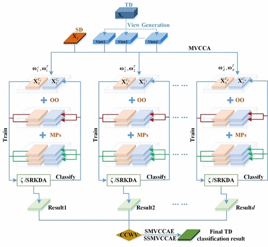
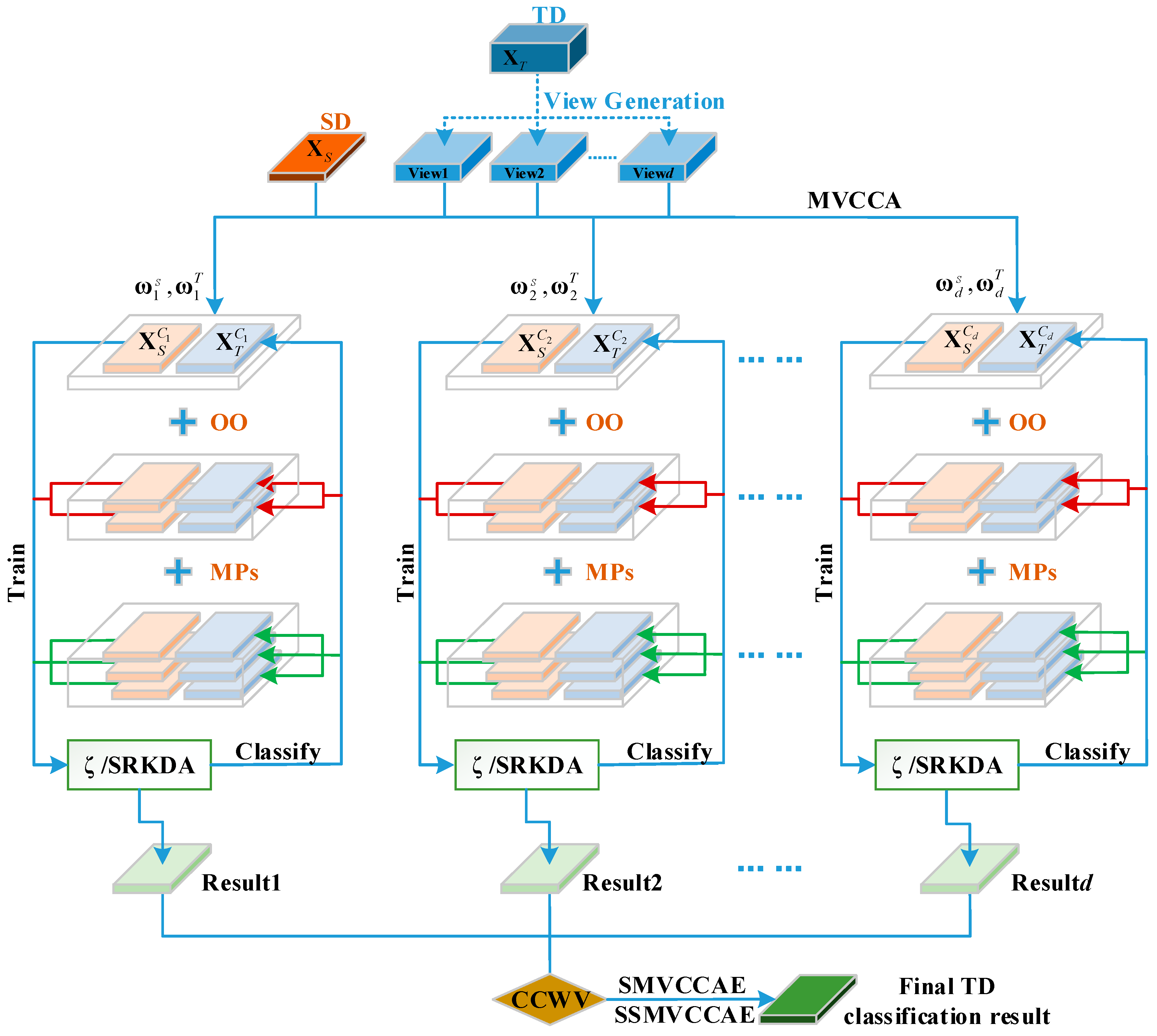
36]. Accordingly, this work introduces an EL technique based on supervised multi-view CCA, which is called supervised multi-view canonical correlation analysis ensemble (SMVCCAE), and we prove its effectiveness for DA (and specifically heterogeneous DA) problems.
Additionally, in real applications, it is typical to experience situations in which there are very limited or even no labeled samples available. In this case, a semi-supervised learning (SSL) technique (e.g., [37]), which uses of unlabeled data to improve performance using a small amount of labeled data from the same domain, might be an appropriate solution. As a matter of fact, many SSDAs have been proposed. However, most existing studies, such as asymmetric kernel transforms (AKT) [38], domain-dependent regularization (DDR) [32], TCA, SSTCA [14,27], and co-regularization based SSDA [39], were designed for homogeneous DA. Very recently, Li et al. [18] proposed a semi-supervised heterogeneous DA by convex optimization of standard multiple kernel learning (MKL) with augmented features. Unfortunately, this optimization is quite challenging in real-world applications. This work instead proposes a semi-supervised version of the above-mentioned multi-view canonical correlation analysis ensemble (called SSMVCCAE), incorporating multiple speed-up spectral regression kernel discriminant analysis (SRKDA) [40] into the original supervised algorithm.

2. Related Work

2.1. Notation for HDA

According to the technical literature, feature-based approaches to HDA can be grouped into the following three clusters, depending on the features used to connect the target and the SD:
(1)
If data from the source and target domains share the same features [41,42,43], then latent semantic analysis (LSA) [44], probabilistic latent semantic analysis (pLSA) [45], and risk minimization techniques [46] may be used.
(2)
If additional features are needed, “feature augmentation” approaches have been proposed, including the method in [37], HFA and SHFA [18], manifold alignment [31], sampling geodesic flow (SGF) [47], and geodesic flow kernel (GFK) [16,30]. All of these approaches introduce a common subspace for the source and target data so that heterogeneous features from both domains.
(3)
If features are adapted across domains through learning transformations, feature transformation-based approaches are considered. This group of approaches includes the HSMap [48], the sparse heterogeneous feature representation (SHFR) [49], and the correlation transfer SVM (CTSVM) [29]. The algorithms that we propose fit into this group.
Although all of the approaches reviewed above have achieved promising results, they also have some limitations of all the approaches reviewed above. For example, the co-occurrence features assumption used in [41,42,43] may not hold in applications such as object recognition, which uses only visual features [32]. For the feature augmentation based approaches discussed in [18,30,31], the domain-specific copy process always requires large storage space, and the kernel version requires even more space and computational complexity because of the parameter tuning. Finally, for the feature transformation based approaches proposed in [29,32,48], they do not optimize the objective function of a discriminative classifier directly, and the computational complexity is highly dependent on the total number of samples or features used for adaptation [12,19].
In this work, we assume that there is only one SD ( S D ) and one TD ( T D ). We also define X S = [ x 1 S , ... , x n S S ] d S × n S and X T = [ x 1 T , ... , x n T T ] d T × n T as the feature spaces in the two domains, with the corresponding marginal distributions p ( X S ) and p ( X T ) for S D and T D , respectively. The parameters d S and d T represent the size of x i S , i = 1 , ... , n S and x j T , j = 1 , ... , n T , n S and n T are the sample sizes for X S and X T , and we have S D = { X S , P ( X S ) } , T D = { X T , P ( X T ) } . The labeled training samples from the SD are denoted by { ( x j S , y j S ) | j = 1 n S } , y j S Ω = { ϖ l } l = 1 c , and they refer to c classes. Furthermore, let us consider as “task” Y the task to assign to each element of a set a label selected in a label space by means of a predictive function f , so that ϒ = { y , f } .
In general, if the feature sets belong to different domains, then either X S X T or p ( X S ) p ( X T ) , or both. Similarly, the condition ϒ S ϒ T implies that either Y S Y T ( Y S = [ y 1 S , ... , y n S S ] , Y T = [ y 1 T , ... , y n T T ] ) or p ( Y S | X S ) p ( Y T | X T ) , or both. In this scenario, a “domain adaptation algorithm” is an algorithm that aims to improve the learning of the predictive function f T in the TD T D using the knowledge available in the SD S D and in the learning task ϒ S , when either S D T D or ϒ S ϒ T . Moreover, in heterogeneous problems, the additional condition d S d T holds.

2.2. Canonical Correlation Analysis

Let us now assume that n S = n T for the feature sets (called “views” here) in the source and target domains. The CCA is the procedure for obtaining the transformation matrices ω S and ω T which maximize the correlation coefficient between the two sets [50]:
max ω S , ω T ρ = ω S Σ S T ω T ω S Σ S S ω S ω T Σ T T ω T
where Σ S T = X S X T , Σ S S = X S X S , Σ T T = X T X T , ρ [ 0 , 1 ] , and “ ” means the matrix transpose. In practice, ω S can be obtained by a generalized eigenvalue decomposition problem:
Σ S T ( Σ T T ) 1 Σ S T ω S = η ( Σ S S ) ω S
where η is a constraint factor. Once ω S is obtained, ω T can be obtained by Σ T T 1 Σ S T ω S / η . By adding the regularization terms λ S Ι and into Σ S S and Σ T T to avoid overfitting and singularity problems, Equation (2) becomes:
Σ S T ( Σ T T + λ T Ι ) 1 Σ S T ω S = η ( Σ S S + λ S Ι ) ω S
As a result, the source and target view data can be transformed into correlation subspaces by:
X S C = X S · ω S , ω S d S × d
X T C = X T · ω T , ω T d T × d
Note that one can derive more than one pair of transformation matrices { ω i S } i = 1 d and { ω i T } i = 1 d , where d = min { d S , d T } is the dimension of the resulting CCA subspace. Once the correlation subspaces X S C and X T C spanned by ω S and ω T are derived, test data in the target view can be directly labeled by any model Μ S C that is trained using the source features X S C .

2.3. Fusion Methods

If multiple “views” are available, then for each view, a label can be associated with each pixel used, for instance, CCA. If multiple labels are present, then they must be fused to obtain a single value using a so-called decision-based fusion procedure. Decision-based fusion aims to provide the final classification label for a pixel by combining the labels obtained, in this case, by multiple view analysis. This usually is obtained using two classes of procedures: weighted voting methods and meta-learning methods [51].
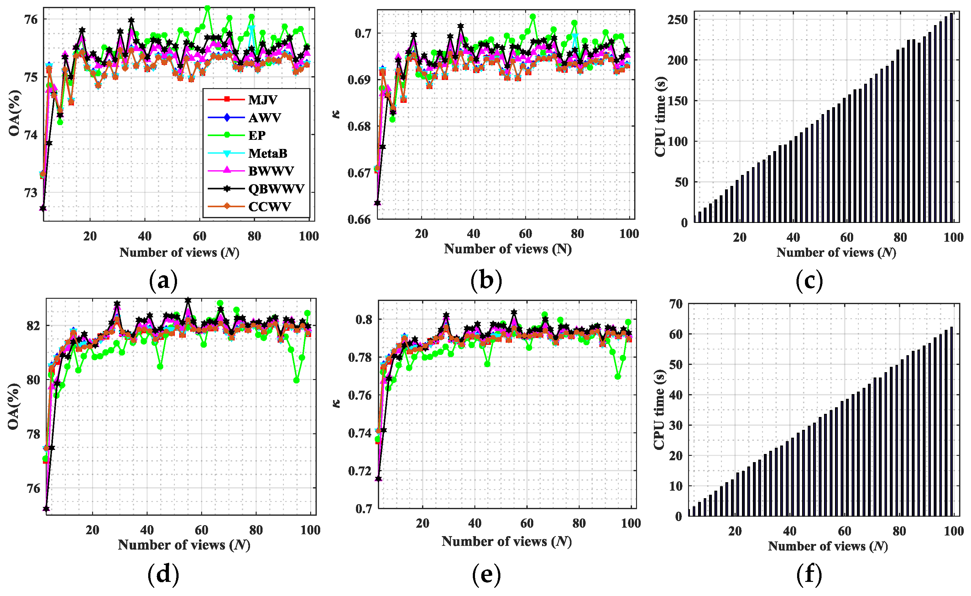
For weighted voting, the labels are combined using the weights assigned to each result. Many variants have been proposed in past decades. For the sake of comparison and because we must consider these options to evaluate the performance of the canonical correlation weighted voting (CCWV) scheme proposed in this paper, here, we consider only the following state-of-the-art techniques:
  • Accuracy weighted voting (AWV), in which the weight of each member is set proportionally to its accuracy performance on a validation set [51]:
    w i = a i j = 1 T a j
    where ai is a performance evaluation of the i-th classifier on a validation set.
  • Best–worst weighted voting (BWWV), in which the best and the worst classifiers are given a weight of 1 or 0, respectively [51], and for the ones the weights are compute according to:
    α i = 1 e i min i ( e i ) max i ( e i ) min i ( e i )
    where ei is the error of the i-th classifier on a validation set.
  • Quadratic best–worst weighted voting (QBWWV), that computes the intermediate weights between 0 and 1 via squaring the above-mentioned BWWV:
    α i = ( max i ( e i ) e i max i ( e i ) min i ( e i ) ) 2

3. The (Semi) Supervised Canonical Correlation Analysis Ensemble

3.1. Supervised Procedure

The idea of this procedure is to adopt MVL to decompose the target domain data into multiple disjoint or partial joint feature subsets (views), where each view is assumed to bring complementary information [52]. Next, these multiple views are used for DA, providing multiple matches between the source and the target domains. Eventually, the labeling task in the SD is transferred into the target domain through CCA, and the results of this “multi-view” CCA are combined to achieve a more efficient heterogeneous DA.
Specifically, without loss of generality, let us assume a heterogeneous DA from a low-dimensional X S to a high-dimensional X T , with d S < d T , which requires that X T is decomposed into N views, i.e., X T = { X T i } i = 1 N , X T i d i × n T , d T = i = i N d i . In this case, the implementation of MVCCA corresponds to searching for the following:
arg max ( ω S i , ω T i ) , ... , ( ω S N , ... , ω T N ) ( ρ 1 , ... , ρ N ) = i = 1 N ( ω S i ) Σ S T i ω T i ( ω S i ) Σ S S i ω S i ( ω T i ) Σ T T i ω T i
where Σ S T i = X S ( X T i ) , Σ S S i = X S X S and Σ T T i = X T i ( X T i ) . Generalizing the standard CCA, Equation (9) can be rewritten as:
arg max ( ω S i , ω T i ) , ... , ( ω S N , ... , ω T N ) ( ρ 1 , ... , ρ N ) = i = 1 N ( ω S i ) Σ S T i ω T i      s . t . ( ω S 1 ) Σ S T 1 ω T i = 1 , ... , ( ω S N ) Σ S T N ω T N = 1
As a result, by using the solutions ω S i | i = 1 N and ω T i | i = 1 N , we will have multiple transformed correlation subspaces, each one considering the SD and one of the target “views”:
X S C i = X S · ω S i , ω S i d S × d ^ i
X T C i = X T i · ω T i , ω T i d T × d ^ i
For any new instance of the target domain, i.e., x = { x i } | i = 1 N , x i X T C i , the decision function of this SMVCCAE, trained with labeled training samples { ( x j S C , y j S ) | j = 1 n S } , x j S C X S C i , i = N , can be implemented via majority voting (MV):
H ( x ) = s i g n ( i = 1 N h i ( x i ) ) = { ϖ l ,   if i = 1 N h i l ( x i ) 1 2 k = 1 c i = 1 N h i k ( x i ) r e j e c t , otherwise
However, to further optimize the ensemble results, one can also recall that the canonical correlations ρ = { { ρ 1 , ... , ρ j } | j = 1 d ^ 1 , ... , { ρ 1 , ... , ρ j } | j = 1 d ^ N } obtained together with the transformation matrices ω S i and ω T i provide information about correlation between the SD and each target view. Since larger values of { ρ j } | j = 1 d ^ i { ρ i } | i = 1 N show a greater correlation, this can also be considered a hint to obtain a better domain transfer ability for the corresponding view. We expect that poor correlation values (i.e., low values of j = 1 d ^ i ρ j ) will result in poor domain transfer abilities. Therefore, j = 1 d ^ i ρ j may be used to quantitatively evaluate the domain transfer ability of the transformation matrices ω S i and ω T i . Accordingly, we propose to include the following canonical correlation coefficient in the voting strategy of Equation (13):
H ( x ) = s i g n ( i = 1 N j = 1 d ^ i ρ j h i ( x i ) )
The algorithmic steps of the new algorithm (called Supervised MVCCA Ensemble, or SMVCCAE for short) are summarized in Algorithm 1.
Algorithm 1. Algorithmic details of SMVCCAE.
1. 
Inputs: SD X S = [ x 1 S , ... , x n S S ] d S × n S ; TD X T = [ x 1 T , ... , x n T T ] d T × n T ; id for labeled training samples
2. 
{ ( x j S , y j S ) | j = 1 n S } , y j S Ω = { ϖ l } l = 1 c from X S , where the superscript C represents the number of class types;
3. 
Supervised classifier ζ ; N the number of views of the TD; and min ( d S , d T ) max ( d S , d T ) N .
4. 
Train: for i = 1 to N
5. 
  generate the target domain view X T i d i × n T , d T = i = i N d i ;
6. 
  return the transformation matrices ω S i and ω T i according to Equation (10);
7. 
  obtain the correlation subspaces X S C i and X T C i according to Equations (11) and (12);
8. 
  compute the transformed training samples { ( x j S C , y j S ) | j = 1 n S } from X S C i according to id;
9. 
  train the classifier h i = ζ ( x S C , y S ) ;
10. 
 end
11. 
Output: return the classifier pool { h 1 , ... , h N } ;
12. 
Classification: For a given new instance x = { x i } | i = 1 N , x i X T C i , predict the label according to Equation (14).

3.2. Semi-Supervised Version

To implement a semi-supervised version of the proposed algorithm, the multiple speed-up SRKDA approach has been incorporated into the supervised procedure. SRDKA essentially improves the original idea of the spectral regression proposed in [53] for linear discriminant analysis (LDA), by transforming the eigenvector decomposition based discriminant analysis into a regression framework via spectral graph embedding [40]. For the sake of clarity, we briefly recall here the SRKDA notation before formalizing its implementation in the new procedure.
Given the labeled samples { ( x j S , y j S ) | j = 1 n S } , y j S Ω = { ϖ l } l = 1 c , the LDA objective function is:
a L D A = arg max a ψ b a a ψ w a ψ b = k = 1 c n k ( u ( k ) u ) ( u ( k ) u ) ψ w = k = 1 c ( q = 1 n k ( x q ( k ) u ( k ) ) ( x q ( k ) u ( k ) ) )
where u is the global centroid, n k is the number of samples in the k-th class, u ( k ) is the centroid of the k-th class, x q ( k ) is the q-th sample in the k-th class, and ψ w and ψ b represent the within-class scatter matrix and the between-class scatter matrix respectively, so that the total scatter matrix is computed as ψ t = ψ b + ψ w . The best solutions for Equation (15) are the eigenvectors that correspond to the nonzero eigenvalues of:
ψ b a L D A = λ ψ t a L D A
To address the nonlinearities, the kernel extension of this procedure maps the input data to a kernel Hilbert space through nonlinear positive semi-definite kernel functions, such as the Gaussian kernel K ( x , y ) = exp ( x y 2 / 2 σ 2 ) , the polynomial kernel K ( x , y ) = ( 1 + x y ) d and the sigmoid kernel K ( x , y ) = tanh ( x y + a ) . Generalizing Equation (15), the projective function of KDA is therefore:
υ K D A = arg max υ ψ b ϕ υ υ ψ t ϕ υ ψ b ϕ = k = 1 c n k ( u ϕ ( k ) u ϕ ) ( u ϕ ( k ) u ϕ ) ψ w ϕ = k = 1 c ( q = 1 n k ( ϕ ( x q ( k ) ) u ϕ ( k ) ) ( ϕ ( x q ( k ) ) u ϕ ( k ) ) ) ψ t ϕ = ψ b ϕ + ψ w ϕ
where ψ b ϕ , ψ w ϕ , and ψ t ϕ denote the between-class, within-class and total scatter matrices in the kernel space, respectively.
Because the eigenvectors of ψ b ϕ υ K D A = λ ψ t ϕ υ K D A are linear combinations of ϕ ( x q ) [54], there is always a coefficient ε q such as υ K D A = q = 1 n k ε q ϕ ( x q ) . This constrain makes Equation (17) equivalent to:
ε K D A = arg max ε K W K ε ε K K ε
where ε K D A = [ ε 1 , ... , ε n k ] . Then, the corresponding eigenproblem becomes:
K W K ε K D A = λ K K ε K D A
where K is the kernel matrix, and the affinity matrix W is defined using either HeatKernel [55] or the binary weight mode:
W i , j = { 1 / n k , if   x i   and   x j   both   belong   to   the   k th   class ; 0 ,        otherwise .
To efficiently solve the KDA eigenproblem in Equation (19), let us consider ϑ to be the solution of W ϑ = λ ϑ . Replacing K ε K D A on the left side of Equation (19) by ϑ , we have:
K W K ε K D A = K W ϑ = K λ ϑ = λ K ϑ = λ K K ε K D A
To avoid singularities, a constant matrix δ I is added to K to keep it positive definite:
ε K D A = ( K + δ I ) 1 ϑ
where I is the identity matrix, and δ 0 represents the regularization parameter. It can be easily verified that the optimal solution given by Equation (22) is the optimal solution of the following regularized regression problem [56]:
min f F j = 1 n S ( f ( x j ) y j ) 2 + δ f K 2
where F is the kernel space associated with the kernel K, and f K is the corresponding norm.
According to Equations (19) and (21), the solution can be reached in two steps: (1) solve the eigenproblem W ϑ = λ ϑ to obtain ϑ ; and (2) find a vector ε K D A that satisfies K ε K D A = ϑ . For Step 1, it is easy to check that the involved affinity matrix W has a block-diagonal structure:
W = [ W ( 1 ) 0 0 0 W ( 2 ) 0 0 0 W ( c ) ]
where { W ( k ) } k = 1 c is an n k × n k matrix with all of the elements defined in Equation (19), and it is straightforward to show that W(k) has the eigenvector e(k) associated with e ( k ) = [ 1 , 1 , ... , 1 ] . In addition, there is only one nonzero eigenvalue of W(k) because the rank of W(k) is always 1. Thus, there are exactly c eigenvectors of W with the same eigenvalue 1:
ϑ k = [ 0 , ... , 0 i = 1 k 1 n i , 1 , ... , 1 n k , 0 , ... , 0 i = k + 1 c n i ]
According to the theorem proven by Cai and He in [57], the kernel matrix is positive definite, and the c-1 projective function of KDA gives exactly the same solutions as the c-1 linear equations systems K ε K D A k = ϑ ¯ k . Then let Θ = [ ε 1 , ... , ε c 1 ] be the KDA transformation matrix which embeds the data into the KDA subspace:
Θ [ K ( : , x 1 ) , ... , K ( : , x n k ) ] = Y ¯
where the columns of Y ¯ are the embedding results. Accordingly, the data with the same label correspond to the same point in the KDA subspace when the kernel matrix is positive definite.
To perform SRKDA in a semi-supervised way, one straightforward solution is to use the label information to guide the construction of the affinity matrix W, as in [57,58,59]. Let G = ( V , E ) be a graph with set of vertices V, which is connected by a set of edges E. The vertices of the graph are the labeled and unlabeled instances ( x j S , y j S ) | j = 1 n S { ( x j T ) | j = 1 n T } . An edge between two vertices (or labeled and unlabeled samples) i, j represents the similarity of two instances with an associated weight {Wi,j}. Then, the affinity matrix W is built using both labeled and unlabeled samples. To achieve this goal, p-nearest neighbors, ε-neighbors, or fully connected graph techniques can be adopted, where 0–1 weighting, Gaussian kernel weighting, Polynomial kernel weighting and Dot-product weighting can be considered to establish the graph weights [57,58]. Usually, graph-based SSL methods compute the normalized graph Laplacian:
L = I D 1 / 2 W D 1 / 2
where D denotes a diagonal matrix defined by D i i = j W i , j (see [59,60] (Chapter 5) for more details on different families of graph based SSL methods).
According to this procedure, and inserting the notation for DA using multiple view CCA, the new semi-supervised procedure follows the steps reported in Algorithm 2.
Algorithm 2. Algorithmic details of SSMVCCAE.
1. 
Inputs: SD X S = [ x 1 S , ... , x n S S ] d S × n S ; TD X T = [ x 1 T , ... , x n T T ] d T × n T ; i d S L for labeled training
2. 
samples { ( x j S , y j S ) | j = 1 n S } , y j S Ω = { ϖ l } l = 1 c from X S , where superscript C represents the number of class
3. 
types; i d T U for unlabeled candidates { ( x j T ) | j = 1 n T } from X T Semi-supervised classifier ζ S R K D A ; N =
4. 
Number of views of the target domain; and min ( d S , d T ) max ( d S , d T ) N .
5. 
Train: for i = 1 to N
6. 
   generate the target domain view X T i d i × n T , d T = i = i N d i ;
7. 
   return the transformation matrices ω S i and ω T i according to Equation (10);
8. 
   obtain the correlation subspaces X S C i and X T C i according to Equations (11) and (12);
9. 
   compute the transformed training samples { ( x j S C , y j S ) | j = 1 n S } from X S C i according to i d S L and the
10. 
   transformed unlabeled samples { ( x j T C ) | j = 1 n T } from X T according to i d T U ;
11. 
   build the graph Laplacian L i according to Equation (27) using ( x j S C , y j S C ) | j = 1 n S { ( x j T C ) | j = 1 n T } ;
12. 
   obtain the KDA transformation matrix Θ i according to the solutions of Equation (26) and Equation (22);
13. 
   return the embedded results Y ¯ i ;
14. 
   end
15. 
Output: return the KDA transformation matrices { Θ i } i = 1 N and the full KDA subspace embedded results { Y ¯ i } i = 1 N ;
16. 
Classification: For a given new instance x = { x i } | i = 1 N , x i X T C i
17. 
for i = 1 to N
18. 
   first map x i into RKHS with the specified kernel function ϕ ( x i ) ;
19. 
   obtain the embedded results Y ¯ i T in KDA space according to Equation (26);
20. 
   return the decision function h i ( x ) = arg min j = 1 c ( y ¯ i T u j 2 ) , y ¯ i T Y ¯ i T , and u j = x c i x / | c j | , which represents the class center of ci in the KDA embedded space.
21. 
end
22. 
obtain the final predicted label by a majority voting ensemble strategy using Equation (14).
Summing up algorithmic details of the SMVCCAE and SSMVCCAE as described in Section 3.1 and Section 3.2, Figure 1 illustrate the general flowchart for the proposed heterogeneous DA algorithms for RS image classification.

4. Data Sets and Setups

4.1. Datasets

For our analyses and evaluations, we consider two datasets, with different spatial and spectral resolutions. The first dataset is a 1.3 m spatial resolution image collected by the Reflective Optics Spectrographic Image System (ROSIS) sensor over the University of Pavia, with a size of 610 × 340 pixels (Figure 2). A total of 103 spectral reflectance bands that cover a region of the spectrum between 430 and 860 nm were retained for the analyses. The captured scene primarily represents a built-up setting with these thematic classes: asphalt, meadows, gravel, trees, metal sheets, bitumen, bare soil, bricks and shadows, as listed in Table 1. As described earlier, the main purpose of this article is to investigate the proposed methods in a heterogeneous DA problem. In this sense, the low-dimensional image is simulated by clustering the spectral space of the original ROSIS image. Specifically, the original bands of the original ROSIS image are clustered into seven groups using the K-Means algorithm, and the mean value of each cluster is considered as a new spectral band, providing a total of seven new bands. In the experiments, the new synthetic image is considered as the SD, whereas the original ROSIS image is considered as the TD.
The second dataset was gathered by the AVIRIS sensor over the Indian Pines test site in North-western Indiana in 1992, with 224 spectral reflectance bands in the wavelength range of 0.4 to 2.5 µm. It consists of 145 × 145 pixels with moderate spatial resolution of 20 m per pixel, and a 16-bit radiometric resolution. After an initial screening, the number of bands was reduced to 200 by removing bands 104–108, 150–163, and 220, due to noise and water absorption phenomena. This scene contains two-thirds agriculture, and one-third forest or other natural perennial vegetation. For the other Pavia data set, K-Means is used to simulate a low dimensional image with 10 bands. For illustrative purposes, Figure 3a,b shows false color composition of the simulated low dimensional and the original AVIRIS Indian Pines scene, whereas Figure 3b shows the ground truth map that is available for the scene, which is displayed in the form of a class assignment for each labeled pixel. In the experimenting stage, this ground truth map is subdivided into two parts for training and validation purposes, as detailed in Table 2.

4.2. Experiment Setups

All of the experiments were performed using MatlabTM on a Windows 10 64-bit system with Intel® CoreTM i7-4970 CPU, @3.60 GHz, 32GB RAM. For the sake of evaluation and comparison, a Random Forest classifier (RaF) is considered as benchmark classifier for both the SMVCCAE and SVCCA approaches, because of its proven velocity, and its generalized and easy-to-implement properties [61,62]. The number of decision trees in RaF is set by default to 100, whereas the number of features is set by default to the floor of the square root of the original feature dimensionality.
For both the ROSIS and Indian Pines data sets, all of the initial and derived features have been standardized to a zero mean and unit variance. For incorporated object oriented (OO), five statistics are utilized, including the pixels’ mean and standard deviation, area, orientation and major axis length of the segmented objects via K-Means clustering algorithm, whereas the spatial feature morphology profiles (MPs) are applied to the three transferred features that have the highest canonical correlation coefficients. Specifically, MPs are constructed by applying closing by reconstruction (CBR) with a circular element with a radius of 3–11 pixels, and opening by reconstruction (OBR) with an element with a radius of 3–6 pixels, refer to works carried out in [63,64]. Therefore, the feature dimensionality set in the experiments is 7 (10) vs. 103 (200) when using spectral features only for ROSIS (Indian Pines), 7 + 5 (10 + 5) vs. 103 + 5 (200 + 5) when using spectral features stacked with OO ones, 7 + 39 (10 + 39) vs. 103 + 39 (200 + 39) when using spectral features stacked with MPs features, and finally 7 + 5 + 39 (10 + 5 + 39) vs. 103 + 5 + 39 (200 + 5 + 39) when using all spectral, OO, and MPs features.
To assess the classification performances of the proposed semi-supervised approach, two state-of-the-art semi-supervised classifiers, Logistic label propagation (LLP) [65] and Laplacian support vector machine (LapSVM) [66] were considered. For the critical parameters of the semi-supervised technique (SRKDA), such as the regularization parameter δ and the number of neighbors NN used to construct the graph Laplacian L with HeatKernel [40], their values are obtained by a heuristic search in the (0.01–1) and (1–15) ranges, respectively. The parameter settings for LLP and LapSVM are instead reported in Table 3. Because LapSVM was originally proposed for binary classification problems, a one-against-all (OAA) scheme was adopted to handle the multiclass classification in our experiments.

5. Experimental Results and Discussion

5.1. Domain Transfer Ability of MVCCA

As discussed in Section 3.1, each dimension in the derived CCA subspace is associated with a different canonical correlation coefficient which is a measure of its transfer ability. Moreover, in the MVCCA scenario, the transfer ability of each view and dimension is controlled not only by the number of views but also by the view generation technique. In this sense, Figure 4 presents the results of the average canonical correlation coefficient obtained using different view generation techniques, i.e., disjoint random sampling, uniform slice, clustering and partially joint random generation. Partially joint random view generation can apparently increase the chance of finding views with better domain transfer ability on the one hand, and to overcome the limitation ensemble techniques when the number of classifiers (equal to number of views in our case) is small on the other hand. Please note that for a more objective evaluation and comparison, each experiment was executed 10 times independently.
In Figure 4, we see that the embedded features with the highest canonical correlation coefficient are obtained by directly applying CCA without multi view generation (i.e., n = 1). However, single view CCA may still fail to balance potential mismatches across heterogeneous domains by overfitting, as demonstrated in the results reported in the following sections. Additionally, the decreasing trend of the canonical correlation coefficient with an increasing number of views is obvious because of the increasing mismatch between the source and target views. However, the decreasing rates of the canonical correlation coefficient for disjoint random and partially joint random generation techniques are lower than those from disjoint uniform slice and disjoint clustering view generations. Therefore, partially joint random and disjoint random view generation techniques have been selected for the following experiments.

5.2. Parameter Analysis for SMVCCAE

In Figure 5, we report the results of a sensitivity analysis of SMVCCAE that involves its critical parameters: the dimension of the target view d T i = d T N , the view generating strategies including disjoint random (DJR) and partially joint random (PJR) generation, as well as the ensemble approaches MJV and CCWV. Please note that the number of views for PJR based SMCCAE was set to 35, which is a number that will be discussed later in this paper.
As illustrated in Figure 5 for the test data sets, the choice of PJR view generation with MJV and CCWV strategies allows the best overall accuracy values (OA curves in color green and pink). Concerning the dimensionality of the target views, they are different using different features. Specifically, for spectral features, the larger the dimensionality of the target views, the larger the OA values for PJR-based SMVCCAE because of the better domain transfer capacity with more ensemble classifiers. However, a dimensionality that is too large leads to too few view splits, i.e., a small number of ensemble elements, eventually resulting in a degraded performance. For example, when target view dimensionality is larger than four times the source view (7) dimensionality for ROSIS and larger than six times this value for Indian Pines, the OA value exhibits a decreasing trend (Figure 5a,e). Among the different types of features, (e.g., spectral and object-oriented features (labeled “spectral-OO”), spectral and morphological profile features (labeled “spectral-MPs”), and all of them together (labeled “spectral-OO-MPs”), the outcome is as expected, which is that the best results are obtained using spectral-OO-MPs. Interestingly, whereas the classification performances of the PJR-based approach are quite stable with respect to the dimensionality of the target views, the DJR-based results show a negative trend with an increasing number of target views. This finding is especially true when spatial (i.e., OO and morphological profiles) features are incorporated. This result can be explained by the trade-off between the diversity, OA and number of classifiers in an ensemble system. Specifically, the statistical diversity among spectral and spatial features tends to enhance the classification accuracy diversities more than using any view splitting strategy. As a result, the final classification performance could be limited or even degraded, especially when the number of classifiers is small.
Finally, in Figure 6, we focus on the computational complexity of the proposed approach by presenting OA, kappa statistics and CPU time values with respect to the number of views and the various fusion strategies.
According to Figure 6, the proposed CCWV fusion technique is effective as the other fusion techniques. Apparently, with regard to the improvements in the OA values (see Figure 6a,b,d,e), and the computational burden from the number of views (see Figure 6c,f), views between 30 and 40 produce the best tradeoff between computational burden and classification accuracy.
In summary, in a scenario in which low-dimensional and high-dimensional data sets require DA, a well-designed SMVCCAE requires us to set the dimensionality of each target view to three or four times the dimensionality of the source view, and to use a PJR view generation technique.

5.3. Validation of SMVCCAE

Figure 7 provides the SMVCCAE heterogeneous cross-domain classification maps with OA values for the ROSIS University dataset using spectral, spectral-OO, spectral-MPs and spectral-OO-MPs features. Compared with the maps produced by a single-view canonical correlation analysis (SVCCA) approach, the thematic maps obtained by SMVCCAE using the associated features are better, specifically with adequate delineations of the bitumen, gravel and bare soil areas (see the numbers in Table 4). These results experimentally verify our earlier assumptions that single view CCA could fail to balance potential mismatches across heterogeneous domains by overfitting. Additionally, the most accurate result is obtained with spectral-OO-MPs by SMVCCAE using the PJR view generation strategy, as shown by the results in Figure 7 and the numbers in bold in Table 4.
For the Indian Pines dataset, Figure 8 shows the thematic maps with OA values, whereas Table 5 reports the classification accuracies (Average accuracy (AA) and OA), and kappa statistics (k) with respect to various features. Once again, the thematic maps with larger OA values produced by SMVCCAE are better than the results produced by SVCCA, especially when the OO and MPs are incorporated. The numbers in bold in Table 5 show that the largest accuracies for various class types are obtained by the SMVCCAE with the PJR technique using spectral-OO-MPs features.

5.4. Parameter Analysis for the Semi-Supervised Version of the Algorithm

In Figure 9 and Figure 10, we report the results of the sensitivity analysis for SSMVCCAE while considering the two critical parameters from the adopted SRKDA technique: (1) the regularization parameter δ; and (2) the number of neighbors NN used to construct the graph Laplacian L. The other parameters, such as the target view dimensionality, d T i and the number of total views N (i.e., the ensemble size), are set by default to d T i = 4 × d s and N = 35, according to our previous experimental analysis for the supervised version of the same technique.
According to the results, the smaller the regularization parameter δ is and the larger the number of neighbors NN, the larger the OA values. Thus, δ = 0.01 and NN = 12 were considered in all of the experiments. Computational complexity is primarily controlled by the labeled sample size (note the vertical axis in Figure 9d–f and Figure 10d–f.

5.5. Validation of the Semi-Supervised MVCCAE

To validate the performances of the semi-supervised version of the proposed algorithm, comparisons with existing methods, specifically LLP and LapSVM, are presented for the ROSIS University data set, starting from a label set of increasing size.
Figure 11 shows the learning curves for SSMVCCAE, LLP, and LapSVM using different view generation and classifier ensemble strategies as a function of this size. Each point on the x-axis represents the size of the labeled samples (pixels) for each class type, while the y-axis represents the average overall classification accuracy. In Table 6, we report the average overall classification accuracies and kappa statistics (κ) over 10 independent runs, when a total of 100 labeled samples are considered for each class.
According to the results in Figure 11 and Table 6, the proposed semi-supervised heterogeneous DA approach achieves comparable and sometimes better results in any case (see the learning curves in blue for SSMVCCAE-SRKDA vs. green for SSMVCCAE-LPP and red for SSMVCCAE-LapSVM in Figure 11). Moreover, larger OA values with faster convergence rates are shown by SSMVCCAE with PJR as opposed to DJR view generation, either by MJV fusion or by the CCWV fusion, especially using the spectral-OO-MPs features.
In Figure 12 and Table 7, the results of the same experiments are reported for the Indian Pines test set. Please note that because only a few samples are available for some classes in the Indian Pines case, class types that contain less than 70 pixels for training are not considered here. Even in this case, to obtain a more objective comparison and evaluation, each test is executed independently for 10 rounds.
Figure 12 shows that better classification results are obtained by the SSMVCCAE with SRKDA, not only using the original spectral features but also using spectral features that incorporate OO and MPs features (see the learning curves in blue vs. those in green and red). Moreover, the best classification results are obtained by SSMVCCAE-SRKDA with the PJR view generation technique, and when considering the spectral-OO-MPs stacked features (see the numbers in bold in Table 7).
Finally, in Figure 13 and Figure 14, the CPU time consumptions in seconds for the different implementations of the semi-supervised procedure are reported as a function of the labeled sample size for both Pavia and Indian Pines. According to the results, SSMVCCAE with SRKDA is only slightly more efficient than LapSVM for the ROSIS University data, but is much more efficient for the Indian Pines data. Moreover, the computational complexities of LapSVM and LLP increase linearly with the number of labeled samples, because they are more visible for the Indian Pines data, whereas the CPU time for SRKDA stays almost constant.
Summing the results presented in this section, it can be concluded that the novel proposed semi-supervised heterogeneous DA approach works properly and achieves satisfactory results better than the current state-of-the-art techniques when using a PJR view generation technique either with majority voting or with canonical correlation coefficient voting. A comparison of the results by SSMVCCAE with those by LLP and LapSVM shows that the performance of SRKDA is superior for both classification accuracy and computational efficiency. Finally, the computational burden caused by the sizes of the labeled samples and feature dimensionality is much smaller for SSMVCCAE with SRKDA, whereas it increases linearly with the sample size when using the other techniques.

6. Conclusions

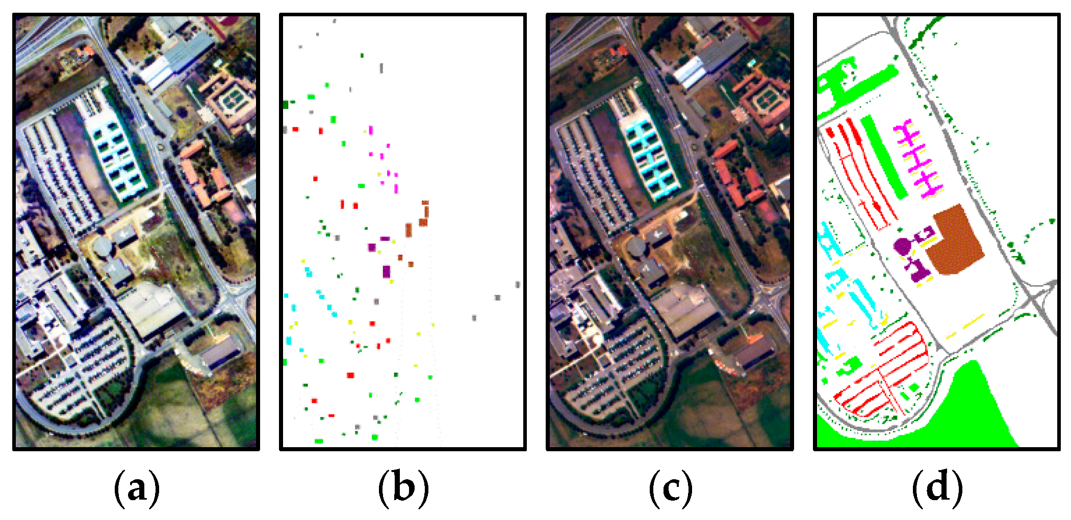
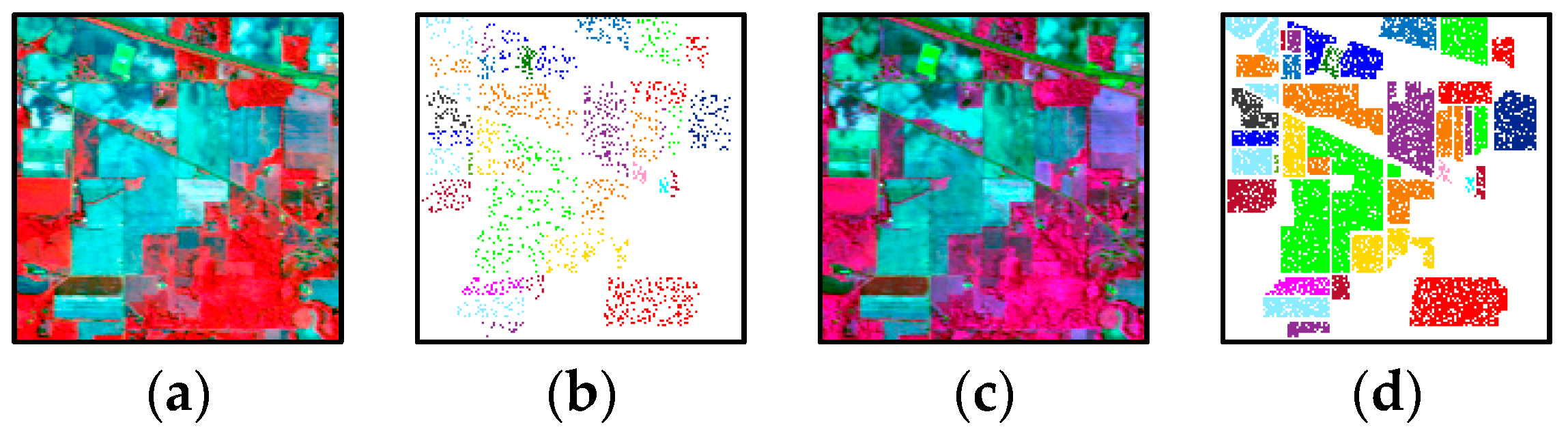
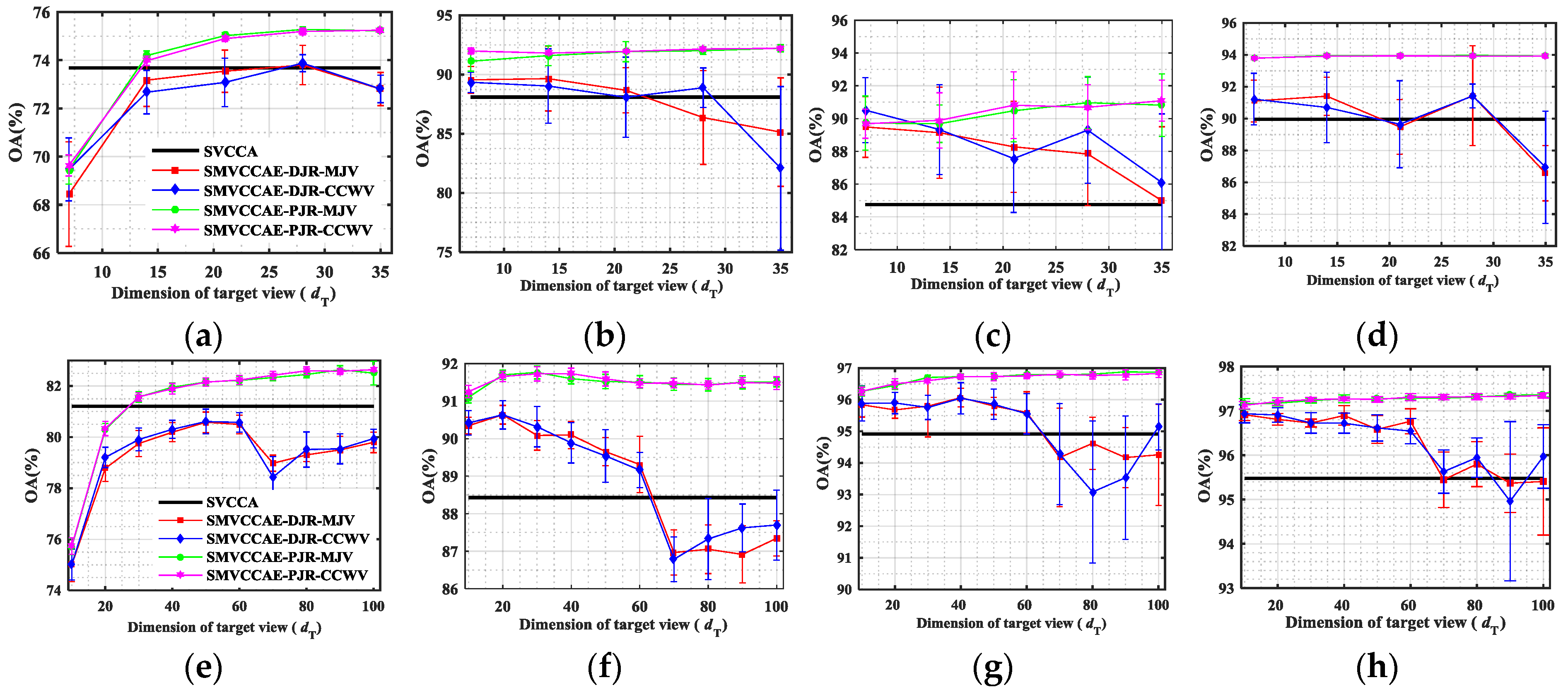
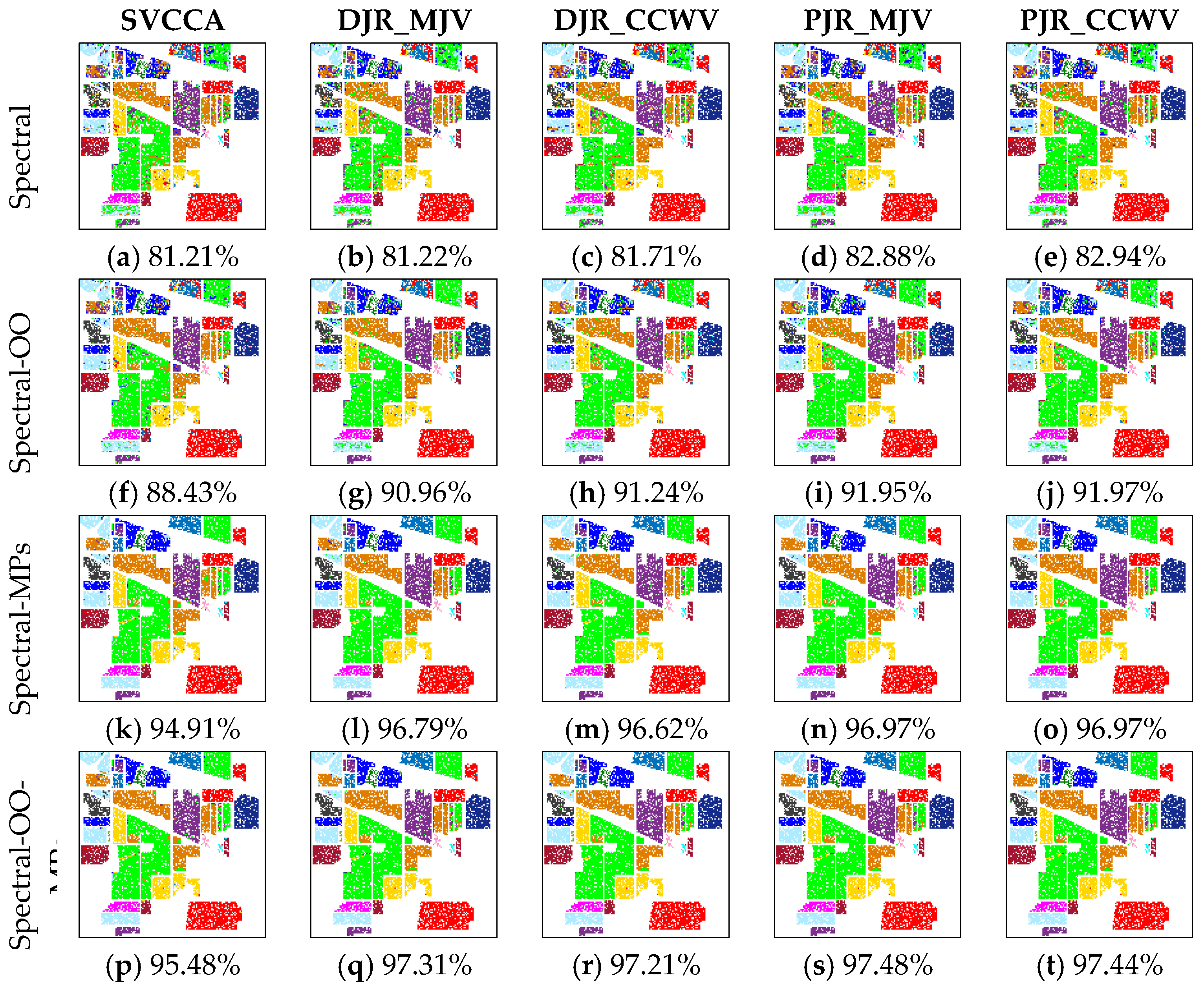
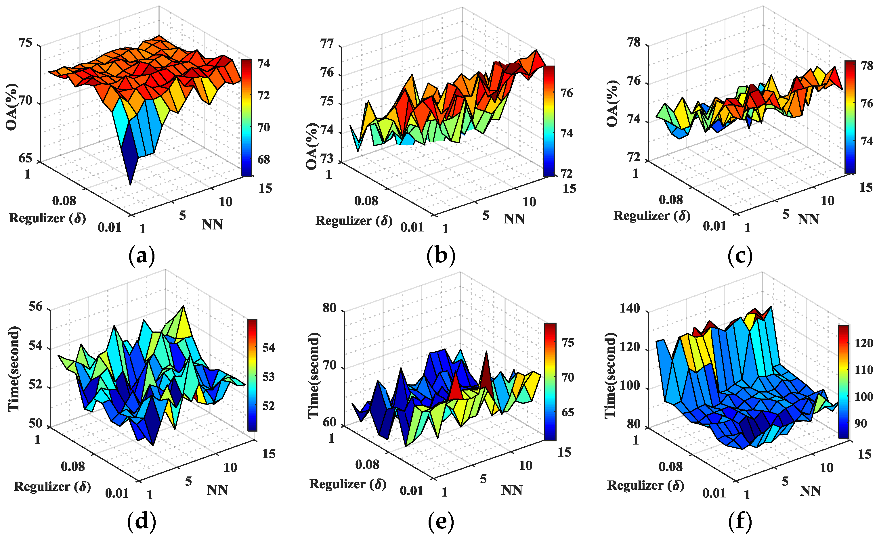
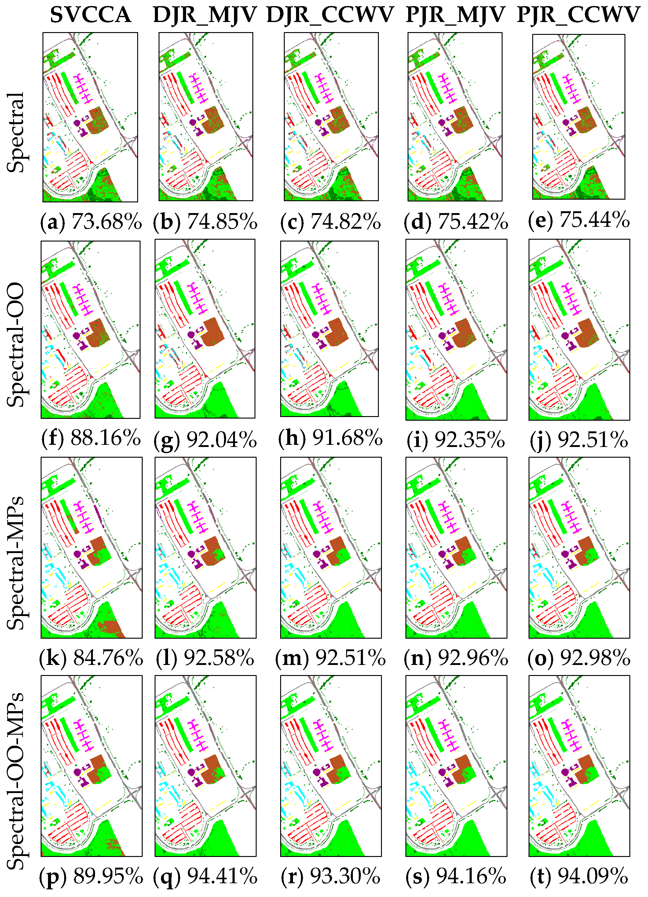
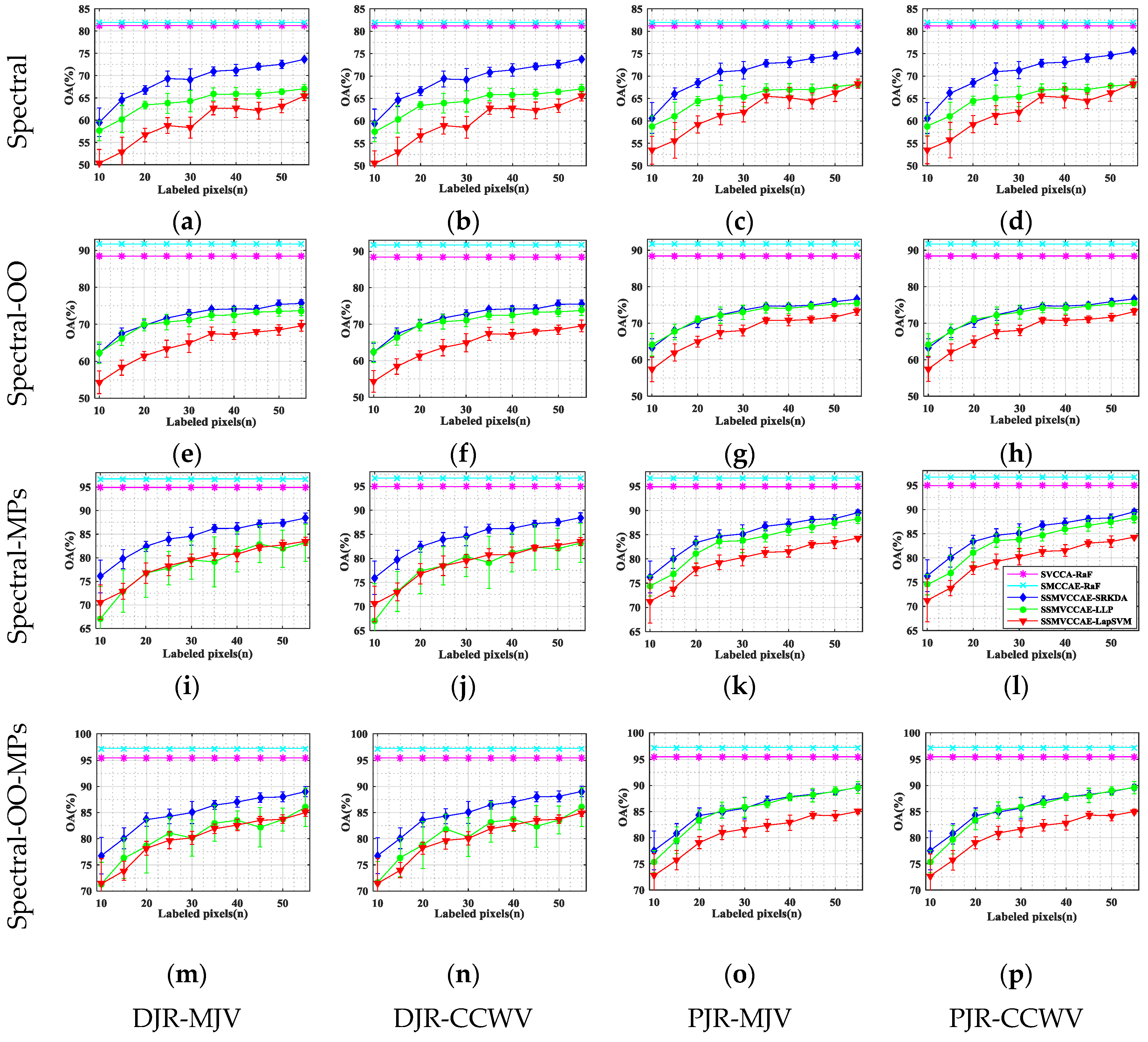
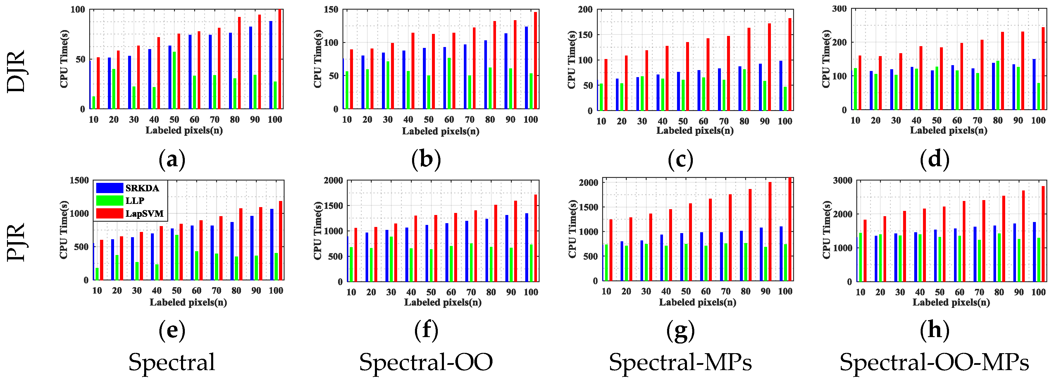
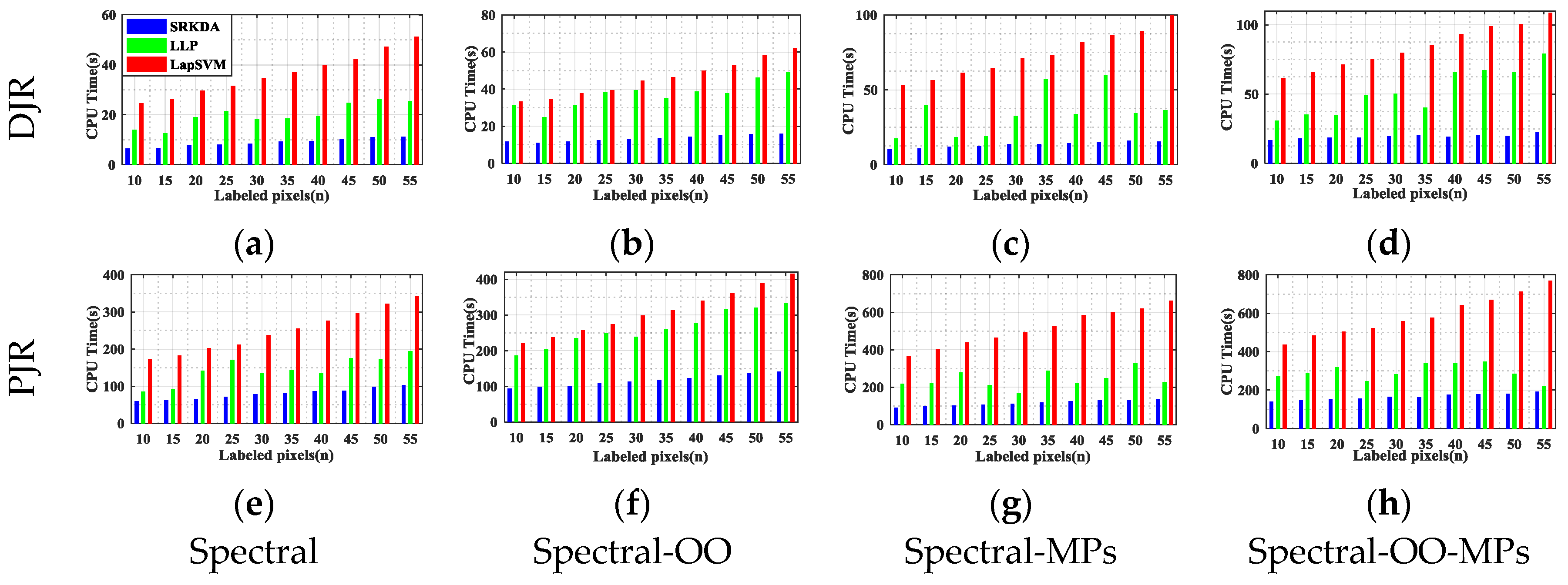
In this paper, we have presented the implementation details, analyzed the parameter sensitivity, and proposed a comprehensive validation of two versions of an ensemble classifier that is suitable for heterogeneous DA and based on multiple view CCA. The main idea is to overcome the limitations of SVCCA by incorporating multi view CCA into EL. Superior results have been proven using two high dimensional (hyperspectral) images, the ROSIS Pavia University and the AVIRIS Indian Pine datasets, as high dimensional target domains, with synthetic low dimensional (multispectral) images as associated SDs. The best classification results were always obtained by jointly considering the original spectral features stacked with object-oriented features assigned to segmentation results, and the morphological profiles, which were subdivided into multiple views using the PJR view generation technique.
To further mitigate the marginal and/or conditional distribution gap between the source and the target domains, when few or even no labeled samples are available from the target domain, we propose a semi-supervised version of the same approach via training multiple speed-up SRKDA.
For new research directions, we are considering more complex problems, such as single SD vs. multiple TDs, as well as multiple SDs vs. multiple TDs supervised and semi-supervised adaptation techniques.

Acknowledgments

This work was partially supported by the Project funded by China Postdoctoral Science Foundation (2016M592872), the Xinjiang Uyghur Autonomous Region High Level Talents Introduction Project (Y648031) and the National Natural Science Foundation of China (No. 41601440, No. 41601354, and No. 41471098).

Author Contributions

Alim Samat developed the algorithms, executed all of the experiments, finished the original manuscript and the subsequent revisions, and provided part of the funding. Claudio Persello and Paolo Gamba offered valuable suggestions and comments, and carefully revised the original manuscript and its revisions. Jilili Abuduwaili provided part of the funding. Sicong Liu and Erzhu Li, contributed to revising of the manuscript.

Conflicts of Interest

The authors declare no conflict of interest.

References

  1. Olofsson, P.; Foody, G.M.; Herold, M.; Stehman, S.V.; Woodcock, C.E.; Wulder, M.A. Good practices for estimating area and assessing accuracy of land change. Remote Sens. Environ. 2014, 148, 42–57. [Google Scholar] [CrossRef]
  2. Curlander, J.C. Location of spaceborne SAR imagery. IEEE Trans. Geosci. Remote Sens. 1982, 3, 359–364. [Google Scholar] [CrossRef]
  3. Bruzzone, L.; Cossu, R. A multiple-cascade-classifier system for a robust and partially unsupervised updating of land-cover maps. IEEE Trans. Geosci. Remote Sens. 2002, 40, 1984–1996. [Google Scholar] [CrossRef]
  4. Torralba, A.; Efros, A.A. Unbiased Look at Dataset Bias. In Proceedings of the IEEE Conference on Computer Vision and Pattern Recognition, Colorado Springs, CO, USA, 20–25 June 2011; pp. 1521–1528. [Google Scholar]
  5. Khosla, A.; Zhou, T.; Malisiewicz, T.; Efros, A.A.; Torralba, A. Undoing the Damage of Dataset Bias. In Proceedings of the IEEE Conference on Computer Vision and Pattern Recognition, Providence, RI, USA, 20–25 June 2012; Springer: Berlin/Heidelberg, Germany, 2012; pp. 158–171. [Google Scholar]
  6. Schott, J.R.; Salvaggio, C.; Volchok, W.J. Radiometric scene normalization using pseudoinvariant features. Remote Sens. Environ. 1988, 26, 1–16. [Google Scholar] [CrossRef]
  7. Woodcock, C.E.; Macomber, S.A.; Pax-Lenney, M.; Cohen, W.B. Monitoring large areas for forest change using Landsat: Generalization across space, time and Landsat sensors. Remote Sens. Environ. 2001, 78, 194–203. [Google Scholar] [CrossRef]
  8. Olthof, I.; Butson, C.; Fraser, R. Signature extension through space for northern landcover classification: A comparison of radiometric correction methods. Remote Sens. Environ. 2005, 95, 290–302. [Google Scholar] [CrossRef]
  9. Rakwatin, P.; Takeuchi, W.; Yasuoka, Y. Stripe noise reduction in MODIS data by combining histogram matching with facet filter. IEEE Trans. Geosci. Remote Sens. 2007, 45, 1844–1856. [Google Scholar] [CrossRef]
  10. Inamdar, S.; Bovolo, F.; Bruzzone, L.; Chaudhuri, S. Multidimensional probability density function matching for preprocessing of multitemporal remote sensing images. IEEE Trans. Geosci. Remote Sens. 2008, 46, 1243–1252. [Google Scholar] [CrossRef]
  11. Bruzzone, L.; Marconcini, M. Domain adaptation problems: A DASVM classification technique and a circular validation strategy. IEEE Trans. Pattern Anal. Mach. Intell. 2010, 32, 770–787. [Google Scholar] [CrossRef] [PubMed]
  12. Pan, S.J.; Yang, Q. A survey on transfer learning. IEEE Trans. Knowl. Data Eng. 2010, 22, 1345–1359. [Google Scholar] [CrossRef]
  13. Banerjee, B.; Bovolo, F.; Bhattacharya, A.; Bruzzone, L.; Chaudhuri, S.; Buddhiraju, K.M. A Novel Graph-Matching-Based Approach for Domain Adaptation in Classification of Remote Sensing Image Pair. IEEE Trans. Geosci. Remote Sens. 2015, 53, 4045–4062. [Google Scholar] [CrossRef]
  14. Matasci, G.; Volpi, M.; Kanevski, M.; Bruzzone, L.; Tuia, D. Semisupervised Transfer Component Analysis for Domain Adaptation in Remote Sensing Image Classification. IEEE Trans. Geosci. Remote Sens. 2015, 53, 3550–3564. [Google Scholar] [CrossRef]
  15. Tuia, D.; Persello, C.; Bruzzone, L. Domain Adaptation for the Classification of Remote Sensing Data: An Overview of Recent Advances. IEEE Geosci. Remote Sens. Mag. 2016, 4, 41–57. [Google Scholar] [CrossRef]
  16. Samat, A.; Gamba, P.; Abuduwaili, J.; Liu, S.; Miao, Z. Geodesic Flow Kernel Support Vector Machine for Hyperspectral Image Classification by Unsupervised Subspace Feature Transfer. Remote Sens. 2016, 8, 234. [Google Scholar] [CrossRef]
  17. Daumé, H., III; Kumar, A.; Saha, A. Frustratingly Easy Semi-Supervised Domain Adaptation. In Proceedings of the 2010 Workshop on Domain Adaptation Natural Language Processing, Uppsala, Sweden, 15 July 2010; pp. 53–59. [Google Scholar]
  18. Li, W.; Duan, L.; Xu, D.; Tsang, I.W. Learning with augmented features for supervised and semi-supervised heterogeneous domain adaptation. IEEE Trans. Pattern Anal. Mach. Intell. 2014, 36, 1134–1148. [Google Scholar] [CrossRef] [PubMed]
  19. Patel, V.M.; Gopalan, R.; Li, R.; Chellappa, R. Visual domain adaptation: A survey of recent advances. IEEE Sign. Process. Mag. 2015, 32, 53–69. [Google Scholar] [CrossRef]
  20. Gao, J.; Fan, W.; Jiang, J.; Han, J. Knowledge Transfer via Multiple Model Local Structure Mapping. In Proceedings of the 14th ACM SIGKDD International Conference on Knowledge Discovery and Data Mining, Las Vegas, NV, USA, 24–27 August 2008; pp. 283–291. [Google Scholar]
  21. Jiang, J.; Zhai, C. Instance Weighting for Domain Adaptation in NLP. In Proceedings of the ACL, Prague, Czech Republic, 23–30 June 2007; Volume 7, pp. 264–271. [Google Scholar]
  22. Sugiyama, M.; Nakajima, S.; Kashima, H.; Buenau, P.V.; Kawanabe, M. Direct Importance Estimation with Model Selection and Its Application to Covariate Shift Adaptation. In Advances in Neural Information Processing Systems; Springer: Vancouver, BC, Canada, 2008; pp. 1433–1440. [Google Scholar]
  23. Persello, C.; Bruzzone, L. Active learning for domain adaptation in the supervised classification of remote sensing images. IEEE Trans. Geosci. Remote Sens. 2012, 50, 4468–4483. [Google Scholar] [CrossRef]
  24. Bruzzone, L.; Persello, C. A novel approach to the selection of spatially invariant features for the classification of hyperspectral images with improved generalization capability. IEEE Trans. Geosci. Remote Sens. 2009, 47, 3180–3191. [Google Scholar] [CrossRef]
  25. Pan, S.J.; Kwok, J.T.; Yang, Q. Transfer Learning via Dimensionality Reduction. In Proceedings of the AAAI, 8, Stanford, CA, USA, 26–28 March 2008; pp. 677–682. [Google Scholar]
  26. Long, M.; Wang, J.; Ding, G.; Pan, S.J.; Yu, P.S. Adaptation regularization: A general framework for transfer learning. IEEE Trans. Knowl. Data Eng. 2014, 26, 1076–1089. [Google Scholar] [CrossRef]
  27. Pan, S.J.; Tsang, I.W.; Kwok, J.T.; Yang, Q. Domain adaptation via transfer component analysis. IEEE Trans. Neural Netw. 2011, 22, 199–210. [Google Scholar] [CrossRef] [PubMed]
  28. Mihalkova, L.; Huynh, T.; Mooney, R.J. Mapping and Revising Markov Logic Networks for Transfer Learning. In Proceedings of the AAAI, 7, Vancouver, BC, Canada, 22–26 July 2007; pp. 608–614. [Google Scholar]
  29. Yeh, Y.R.; Huang, C.H.; Wang, Y.C.F. Heterogeneous domain adaptation and classification by exploiting the correlation subspace. IEEE Trans. Image Proc. 2014, 23, 2009–2018. [Google Scholar]
  30. Gopalan, R.; Li, R.; Chellappa, R. Domain Adaptation for Object Recognition: An Unsupervised Approach. In Proceedings of the IEEE International Conference on Computer Vision, Barcelona, Spain, 6–13 November 2011; pp. 999–1006. [Google Scholar]
  31. Gopalan, R.; Li, R.; Chellappa, R. Unsupervised adaptation across domain shifts by generating intermediate data representations. IEEE Trans. Pattern Anal. Mach. Intell. 2014, 6, 2288–2302. [Google Scholar] [CrossRef] [PubMed]
  32. Duan, L.; Xu, D.; Tsang, I.W. Domain adaptation from multiple sources: A domain-dependent regularization approach. IEEE Trans. Neural Netw. Learn. Syst. 2012, 23, 504–518. [Google Scholar] [CrossRef] [PubMed]
  33. Wang, W.; Zhou, Z.H. A New Analysis of Co-Training. In Proceedings of the 27th International Conference on Machine Learning, (ICML-10) 2010, Haifa, Israel, 21–24 June 2010; pp. 1135–1142. [Google Scholar]
  34. Di, W.; Crawford, M.M. View generation for multiview maximum disagreement based active learning for hyperspectral image classification. IEEE Trans. Geosci. Remote Sens. 2012, 50, 1942–1954. [Google Scholar] [CrossRef]
  35. Sun, S. A survey of multi-view machine learning. Neural Comput. Appl. 2013, 23, 2031–2038. [Google Scholar] [CrossRef]
  36. Kuncheva, L.I.; Rodríguez, J.J.; Plumpton, C.O.; Linden, D.E.; Johnston, S.J. Random subspace ensembles for fMRI classification. IEEE Trans. Med. Imaging 2010, 29, 531–542. [Google Scholar] [CrossRef] [PubMed]
  37. Samat, A.; Du, P.; Liu, S.; Li, J. E2LMs: Ensemble extreme learning machines for hyperspectral image classification. IEEE J. Sel. Top. Appl. Earth Obs. Remote Sens. 2014, 7, 1060–1069. [Google Scholar] [CrossRef]
  38. Hady, M.F.A.; Schwenker, F. Semi-Supervised Learning. In Handbook on Neural Information Processing; Springer: Berlin/Heidelberg, Germany, 2013; pp. 215–239. [Google Scholar]
  39. Kulis, B.; Saenko, K.; Darrell, T. What you Saw Is not What you Get: Domain Adaptation Using Asymmetric Kernel Transforms. In Proceedings of the IEEE International Conference on Computer Vision and Pattern Recognition (CVPR), Colorado Springs, CO, USA, 20–25 June 2011; pp. 1785–1792. [Google Scholar]
  40. Kumar, A.; Saha, A.; Daume, H. Co-regularization based semi-supervised domain adaptation. In Advances in Neural Information Processing Systems 23 (NIPS 2010); Springer: Vancouver, BC, Canada, 2010; pp. 478–486. [Google Scholar]
  41. Cai, D.; He, X.; Han, J. Speed up kernel discriminant analysis. VLDB J. Int. J. Very Large Data Bases 2011, 20, 21–33. [Google Scholar] [CrossRef]
  42. Dai, W.; Chen, Y.; Xue, G.R.; Yang, Q.; Yu, Y. Translated learning: Transfer learning across different feature spaces. In Advances in Neural Information Processing Systems; Springer: Vancouver, BC, Canada, 2008; pp. 353–360. [Google Scholar]
  43. Yang, Q.; Chen, Y.; Xue, G.R.; Dai, W.; Yu, Y. Heterogeneous Transfer Learning for Image Clustering via the Social Web. In Proceedings of the Joint Conference 47th Annual Meeting of the ACL and the 4th International Joint Conference Natural Language Process, AFNLP, Singapore, 2–7 August 2009; Volume 1, pp. 1–9. [Google Scholar]
  44. Zhu, Y.; Chen, Y.; Lu, Z.; Pan, S.J.; Xue, G.R.; Yu, Y.; Yang, Q. Heterogeneous Transfer Learning for Image Classification. In Proceedings of the AAAI, San Francisco, CA, USA, 7–11 August 2011. [Google Scholar]
  45. Evangelopoulos, N.; Zhang, X.; Prybutok, V.R. Latent semantic analysis: Five methodological recommendations. Eur. J. Inf. Syst. 2012, 21, 70–86. [Google Scholar] [CrossRef]
  46. Hong, L. A Tutorial on Probabilistic Latent Semantic Analysis. Available online: https://arxiv.org/pdf/1212.3900.pdf (accessed on 21 December 2012).
  47. Koltchinskii, V. Rademacher penalties and structural risk minimization. IEEE Trans. Inf. Theory 2001, 47, 1902–1914. [Google Scholar] [CrossRef]
  48. Gong, B.; Shi, Y.; Sha, F.; Grauman, K. Geodesic Flow Kernel for Unsupervised Domain Adaptation. In Proceedings of the 2012 IEEE Conference Computer Vision and Pattern Recognition (CVPR), Providence, RI, USA, 16–21 June 2012; pp. 2066–2073. [Google Scholar]
  49. Shi, X.; Liu, Q.; Fan, W.; Yu, P.S.; Zhu, R. Transfer Learning on Heterogenous Feature Spaces via Spectral Transformation. In Proceedings of the IEEE 10th International Conference on Data Mining, Sydney, Australia, 13–17 December 2010; pp. 1049–1054. [Google Scholar]
  50. Zhou, J.T.; Tsang, I.W.; Pan, S.J.; Tan, M. Heterogeneous Domain Adaptation for Multiple Classes. In Proceedings of the AISTATS, Reykjavik, Iceland, 22–25 April 2014; pp. 1095–1103. [Google Scholar]
  51. Hardoon, D.R.; Szedmak, S.; Shawe-Taylor, J. Canonical correlation analysis: An overview with application to learning methods. Neural Comput. 2004, 16, 2639–2664. [Google Scholar] [CrossRef] [PubMed]
  52. Rokach, L. Pattern Classification Using Ensemble Methods; World Scientific Publishing Company: Singapore, 2010; Volume 75. [Google Scholar]
  53. Xu, C.; Tao, D.; Xu, C. Multi-View Learning with Incomplete Views. IEEE Trans. Image Proc. 2015, 24, 5812–5825. [Google Scholar] [CrossRef] [PubMed]
  54. Cai, D.; He, X.; Han, J. Spectral Regression: A Unified Subspace Learning Framework for Content-Based Image Retrieval. In Proceedings of the 15th International Conference on Multimedia, Augsburg, Germany, 24–29 September 2007; pp. 403–412. [Google Scholar]
  55. Baudat, G.; Anouar, F. Generalized discriminant analysis using a kernel approach. Neural Comput. 2000, 12, 2385–2404. [Google Scholar] [CrossRef] [PubMed]
  56. Vassilevich, D.V. Heat kernel expansion: User’s manual. Phys. Rep. 2003, 388, 279–360. [Google Scholar] [CrossRef]
  57. Vapnik, V.N. An overview of statistical learning theory. IEEE Trans. Neural Netw. 1999, 10, 988–999. [Google Scholar] [CrossRef] [PubMed]
  58. Cai, D.; He, X.; Han, J. Document clustering using locality preserving indexing. IEEE Trans. Knowl. Data Eng. 2005, 17, 1624–1637. [Google Scholar] [CrossRef]
  59. Subramanya, A.; Talukdar, P.P. Graph-based semi-supervised learning. Synth. Lect. Arti. Intell. Mach. Learn. 2014, 8, 1–125. [Google Scholar] [CrossRef]
  60. Camps-Valls, G.; Marsheva, T.V.B.; Zhou, D. Semi-supervised graph-based hyperspectral image classification. IEEE Trans. Geosci. Remote Sens. 2007, 45, 3044–3054. [Google Scholar] [CrossRef]
  61. Breiman, L. Random forests. Mach. Learn. 2001, 45, 5–32. [Google Scholar] [CrossRef]
  62. Du, P.; Samat, A.; Waske, B.; Liu, S.; Li, Z. Random Forest and Rotation Forest for fully polarized SAR image classification using polarimetric and spatial features. ISPRS J. Photogramm. Remote Sens. 2015, 105, 38–53. [Google Scholar] [CrossRef]
  63. Benediktsson, J.A.; Palmason, J.A.; Sveinsson, J.R. Classification of hyperspectral data from urban areas based on extended morphological profiles. IEEE Trans. Geosci. Remote Sens. 2005, 43, 480–491. [Google Scholar] [CrossRef]
  64. Fauvel, M.; Benediktsson, J.A.; Chanussot, J.; Sveinsson, J.R. Spectral and spatial classification of hyperspectral data using SVMs and morphological profiles. IEEE Trans. Geosci. Remote Sens. 2008, 46, 3804–3814. [Google Scholar] [CrossRef]
  65. Kobayashi, T.; Watanabe, K.; Otsu, N. Logistic label propagation. Pattern Recognit. Lett. 2012, 33, 580–588. [Google Scholar] [CrossRef]
  66. Melacci, S.; Belkin, M. Laplacian support vector machines trained in the primal. J. Mach. Learn. Res. 2011, 12, 1149–1184. [Google Scholar]
Figure 1. General flowchart for the proposed heterogeneous DA algorithms SMVCCAE and SSMVCCAE for RS image classification.
Remotesensing 09 00337 g001
Figure 2. (ad) False color composite of the: synthetic low spectral resolution (a); and the original hyperspectral (c) images of the University campus in Pavia, together with: training (b); and validation (d) data sets (legend and sample details are reported in Table 1). False color composites are obtained and are displayed as R, G, and B bands 7, 5, and 4 for the synthetic, and bands 60, 30, and 2 for the original image, respectively.
Remotesensing 09 00337 g002
Figure 3. (ad) False color composites of the: simulated low spectral resolution (a); and original hyperspectral (c) images of Indian Pines data, together with: training (b); and validation (d) data sets (color legend and sample details are reported in Table 2). False color composites are obtained displaying as R, G, and B bands, 6, 4, and 5 for the synthetic, and bands 99, 51, and 21 for the original image, respectively.
Remotesensing 09 00337 g003
Figure 4. Average canonical correlation coefficient versus embedded features for: ROSIS (ad); and Indian Pines (eh) data sets using different view generation techniques: disjoint random sampling (a,e); uniform slice (b,f); clustering (c,g); and partially joint random generation (d,h).
Remotesensing 09 00337 g004
Figure 5. (ah)Average OA values versus target view dimensionality for SMVCCAE with different fusion strategies using: spectral (a,e); spectral-OO (b,f); spectral-MPs (c,g); and spectral-OO-MPs (d,h) features on: ROSIS University (ad); and Indian Pine datasets (eh).
Remotesensing 09 00337 g005
Figure 6. Average OA, Kappa (κ) and CPU time in seconds vs. the number of views for SMVCCA with PJR view generation and various fusion strategies applied to spectral features of ROSIS: University (ac); and Indian Pines datasets (df).
Remotesensing 09 00337 g006
Figure 7. (at) Summary of the best classification maps with OA values for SMVCCAE with different fusion strategies using spectral, OO and MPs features of ROSIS University.
Remotesensing 09 00337 g007
Figure 8. (at) Summary of the best classification maps with OA values for SMVCCAE with different fusion strategies using spectral, OO and MPs features of Indian Pines.
Remotesensing 09 00337 g008
Figure 9. (af) OA values and CPU time (in seconds) versus the regularization parameter (δ) and nearest neighborhood size (NN) set of SSMVCCAE with DJR view generation strategy for ROSIS University using different sizes of labeled samples: 10 pixels/class (a,d); 50 pixels/class (b,e); and 100 pixels/class (c,f).
Remotesensing 09 00337 g009
Figure 10. (af) OA values and CPU time (in seconds) versus the regularization parameter (δ) and nearest neighborhood size (NN) set of SSMVCCAE with the DJR view generation strategy for Indian Pine using different size of labeled samples: 10 pixels/class (a,d); 30 pixels/class (b,e); and 55 pixels/class (c,f).
Remotesensing 09 00337 g010
Figure 11. (ap) Average OA values versus labeled pixels for SSMVCCAE with different view generation and fusion strategies for ROSIS University dataset.
Remotesensing 09 00337 g011
Figure 12. (ap) Average OA values versus labeled pixels for SSMVCCAE with different view generation and fusion strategies on Indian Pines data.
Remotesensing 09 00337 g012
Figure 13. (ah) CPU time consumption in seconds versus the size of the labeled samples for SSMVCCAE-SRKDA/-LLP/-LapSVM for the ROSIS University data.
Remotesensing 09 00337 g013
Figure 14. (ah) CPU time versus the size of the labeled samples for SSMVCCAE-SRKDA/-LLP/-LapSVM for the Indian Pines data.
Remotesensing 09 00337 g014
Table 1. Class legend and sample details for the ROSIS University data set.
No.ClassCodeSourceTarget
TrainTest
1Asphalt 5486631
2Meadows 54018649
3Gravel 3922099
4Trees 5243064
5Metal sheets 2651345
6Bare soil 5325029
7Bitumen 3751330
8Bricks 5143682
9Shadows 231947
Table 2. Class legend and sample details for the AVIRIS Indian Pines data set.
No.ClassCodeSourceTarget
TrainTest
1Alfalfa 2323
2Corn-notill 2281200
3Corn-mintill 130700
4Corn-notill 57180
5Grass-pasture 83400
6Grass-trees 130600
7Grass-pasture-mowed 1414
8Hay-windrowed 78400
9Oats 1010
10Soybean-notill 172800
11Soybean-mintill 2552200
12Soybean-clean 93500
13Wheat 55150
14Woods 2651000
15Buildings-grass-trees-drives 86300
16Stone-steel-towers 4350
Table 3. Parameter details for LLP and LapSVM.
ClassifierParametersMeaningsValues
LLPggraph complete typeKNN
τneighborhood typeSupervised
Nneighbor size for constructing graph5
ωweights for edge in graphHeat Kernel
σparameter for Heat Kernel1
Cregularization scale0.001
Mmaxim iteration number1000
ηweight function for labeled samplesmean
LapSVMγaregularization parameter (ambient norm)10−5
γiregularization parameter (intrinsic norm)1
αthe initial weights0
κkernel typeRBF
σRBF kernel parameter0.01
Μmaximum iteration number200
cLapSVM training typeprimal
ηLaplacian normalizationTRUE
Nneighbor size for constructing graph6
Table 4. Classification accuracy values for the SVCCA and SMVCCAE (dT = 4 × dS) methods for ROSIS University. Considered metrics: Overall accuracy (OA), Average accuracy (AA), Kappa statistic (Kappa).
MethodsStrategyFeaturesAsphaltMeadowsGravelTreesMetal SheetsBare SoilBitumenBricksShadowsAA (%)OA (%)Kappa
SVCCA~F194.9691.6166.1752.5698.6845.7070.6369.5099.2676.5673.680.67
F298.0295.8893.0471.5998.6871.1390.8876.59100.0088.4288.760.85
F399.4788.0694.3980.8999.5553.1072.3190.6798.9086.3784.760.80
F499.8689.3291.3582.4398.6771.9896.4495.7699.1591.6689.960.87
SMVCCAEDJR_MJVF194.7293.3873.7251.8099.4045.9673.7368.4999.6277.8773.800.68
F295.3597.5977.9361.6899.6182.7481.9468.4599.9085.0286.370.82
F399.3690.5895.8874.9199.3772.6994.7985.2899.2190.2388.160.85
F499.4992.0596.7679.3899.7788.8496.4586.1599.2693.1391.440.89
DJR_CCWVF194.8193.2573.4451.8299.6545.9974.4368.2999.6177.9273.840.68
F296.5698.5678.4562.4799.4792.1688.7468.7999.8187.2288.890.86
F399.3190.6096.0574.2699.5275.2596.4085.8299.3290.7288.330.85
F499.2490.6496.7277.6599.2893.3297.3686.7199.1993.3491.420.89
PJR_MJVF195.3094.3176.8452.4899.8348.1576.3669.2099.8779.1575.280.69
F298.6498.0095.6277.1999.5289.2697.5772.6999.7992.0392.140.90
F399.7291.0998.9682.1599.9380.1099.6287.1199.3693.1190.970.88
F499.8991.4694.9784.6399.9398.8199.3495.6699.4096.0193.970.92
PJR_CCWVF195.2694.3377.4552.4499.8347.9676.5669.0699.8679.1975.200.69
F298.5598.0295.5577.3399.5489.4097.5772.6299.7992.0492.160.90
F399.7190.9099.0882.1499.9577.9499.5686.9999.3692.8590.690.88
F499.8991.3695.1684.4099.9598.8899.3595.7899.3896.0293.920.92
F1: Spectral; F2: Spectral-OO; F3: Spectral-MPs; F4: Spectral-OO-MPs.
Table 5. Classification accuracy values (average) for the SVCCA and SMVCCAE methods for Indian Pines. Considered metrics: Overall accuracy (OA), Average accuracy (AA), Kappa statistic (Kappa).
MethodsSVCCASMVCCAE
Strategy~DJR_MJVDJR_CCWVPJR_MJVPJR_CCWV
FeaturesF1F2F3F4F1F2F3F4F1F2F3F4F1F2F3F4F1F2F3F4
Alfalfa69.5791.3086.9686.9645.2291.3095.2295.6548.2691.3095.6595.6546.0991.3095.6595.6546.0991.3095.6595.65
Corn-notill81.4287.4290.6793.9278.0487.8690.4591.9277.9187.0590.4191.7080.8389.1291.0692.7880.8289.3891.1492.90
Corn-mintill70.7188.7196.8696.5764.7084.5497.0098.1665.3483.2997.3197.9165.8786.5498.0399.2065.4386.9397.9799.24
Corn-notill75.5694.4495.5696.6762.8383.8994.1195.3362.9483.4493.1195.6165.5686.1795.5695.8965.6186.2895.5695.95
Grass-pasture79.0081.5088.7588.7572.9886.4893.1393.6072.9586.3892.5593.7075.9088.6593.6393.9075.9588.4393.7394.00
Grass-trees91.0092.1799.0099.0096.0396.8099.7099.6995.6896.7399.6799.6496.5897.3399.6799.6796.5097.4999.6799.67
Grass-pasture-mowed85.7185.7185.7185.7191.4392.8692.8692.8692.8692.8692.8692.8692.8692.8692.8692.8692.8692.8692.8692.86
Hay-windrowed97.7597.5099.7599.7598.4596.3099.6899.7098.6896.9399.6899.6399.4597.7099.7399.7599.2397.8399.6599.75
Oats90.0090.00100.00100.0080.0089.0091.0099.0085.0092.0097.0098.0091.0099.00100.100.89.0098.00100.100.
Soybean-notill77.7587.3887.2589.0079.3789.8391.3492.5979.5489.0290.9392.2281.8991.8592.2793.1481.7091.8992.1592.92
Soybean-mintill78.5587.4595.7795.6476.9491.2097.3598.4477.2091.2297.5498.1678.5292.8298.1698.5478.7492.8898.2598.52
Soybean-clean71.6082.8093.8093.8073.4281.8695.2096.3673.9082.7295.1895.9477.9086.1097.1497.1677.5086.1696.9097.18
Wheat99.3399.3398.6798.6798.2099.0098.6098.7398.1398.5398.2798.8098.5499.3398.6799.0098.4799.3398.6798.80
Woods96.6096.9099.6099.5098.2398.9499.8799.8298.1798.9099.8399.8598.3799.0899.9199.9198.4199.0699.9099.90
Buildings-grass-trees-drives51.3361.3399.0099.0056.0069.6099.7799.9755.2770.2799.9099.9757.1769.87100.100.56.6070.33100.100.
Stone-steel-towers100.100.100.100.99.80100.100.100.99.60100.100.100.100.100.100.100.100.100.100.100.
AA (%)82.2489.0094.8395.1879.4889.9795.9596.9980.0990.0496.2496.8581.6691.7397.0297.3481.4391.7697.0197.33
OA (%)81.2188.4394.9195.4880.1990.1096.0796.8980.3089.8996.0596.7281.9591.6096.7397.2781.8991.7196.7397.27
Kappa0.780.870.940.950.770.890.950.960.770.880.950.960.790.900.960.970.790.900.960.97
F1: Spectral; F2: Spectral-OO; F3: Spectral-MPs; F4: Spectral-OO-MPs.
Table 6. Average overall classification accuracies and kappa statistics (κ) for SSMVCCAE with different semi-supervised classifiers for the ROSIS University data. Total 100 labeled samples are available for each class over 10 independent runs.
ClassifierSSMVCCAE (SRKDA)SSMVCCAE (LPP)SSMVCCAE (LapSVM)
View GenerationDJRPJRDJRPJRDJRPJR
VotingMJVCCWVMJVCCWVMJVCCWVMJVCCWVMJVCCWVMJVCCWV
StatisticsOAκOAκOAκOAκOAκOAκOAκOAκOAκOAκOAκOAκ
Spectral73.820.6673.830.6674.580.6774.470.6775.120.6875.110.6875.450.6875.370.6872.820.6672.850.6674.260.6774.160.67
Spectral-OO78.310.7278.290.7278.020.7278.000.7282.080.7682.040.7683.440.7883.320.7877.370.7177.380.7180.080.7480.040.74
Spectral-MPs88.230.8588.240.8586.730.8286.890.8388.440.8588.450.8590.160.8790.170.8785.650.8285.720.8288.140.8588.120.85
Spectral-OO-MPs93.170.9193.140.9193.470.9193.460.9190.360.8790.310.8792.780.9092.770.9092.080.9092.100.9093.680.9293.670.92
Table 7. Average overall classification accuracies and kappa statistics (κ) for SSMVCCAE with different semi-supervised classifiers for the Indian Pines data. A total of 55 labeled samples are available for each class over 10 independent runs.
ClassifierSSMVCCAE (SRKDA)SSMVCCAE (LPP)SSMVCCAE (LapSVM)
View GenerationDJRPJRDJRPJRDJRPJR
VotingMJVCCWVMJVCCWVMJVCCWVMJVCCWVMJVCCWVMJVCCWV
StatisticsOAκOAκOAκOAκOAκOAκOAκOAκOAκOAκOAκOAκ
Spectral73.670.7073.810.7075.490.7275.510.7267.050.6267.130.6268.180.6468.170.6465.430.6165.480.6168.340.6468.380.64
Spectral-OO75.640.7275.530.7276.610.7376.660.7373.690.7073.750.7075.420.7275.470.7269.590.6569.540.6573.200.6973.180.69
Spectral-MPs88.420.8788.490.8789.570.8889.540.8883.190.8183.220.8188.290.8688.310.8683.490.8183.510.8184.330.8284.330.82
Spectral-OO-MPs89.020.8789.050.8789.660.8889.660.8886.010.8486.020.8489.600.8889.590.8885.010.8384.990.8385.030.8385.010.83

