
Improving Spatial Coverage for Aqua MODIS AOD using NDVI-Based Multi-Temporal Regression Analysis
by
 , , ,
, , ,
Tianhao Zhang
1 ,
,
Chao Zeng
2,
Wei Gong
1,3,
Lunche Wang
4,*,
Kun Sun
1,
Huanfeng Shen
3,5,
Zhongmin Zhu
1,6,* and
Zerun Zhu
1 1
State Key Laboratory of Information Engineering in Surveying, Mapping and Remote Sensing, Wuhan University, Wuhan 430079, China
2
Department of Hydraulic Engineering, Tsinghua University, Beijing 100084, China
3
Collaborative Innovation Center for Geospatial Information Technology, Wuhan 430079, China
4
Laboratory of Critical Zone Evolution, School of Earth Sciences, China University of Geosciences, Wuhan 430074, China
5
School of Resource and Environmental Sciences, Wuhan University, Wuhan, China
6
College of Information Science and Engineering, Wuchang Shouyi University, Wuhan 430064, China
*
Authors to whom correspondence should be addressed.
Remote Sens. 2017, 9(4), 340; https://doi.org/10.3390/rs9040340
Submission received: 3 February 2017
/
Revised: 23 March 2017
/
Accepted: 1 April 2017
/
Published: 2 April 2017
Abstract
:The Moderate Resolution Imaging Spectroradiometer (MODIS) provides widespread Aerosol Optical Depth (AOD) datasets for climatological and environmental health research. Since MODIS AOD clearly lacks coverage in orbit-scanning gaps and cloud obscuration, some applications will benefit from data recovery using multi-temporal AOD. Aimed at qualitatively describing the relationship between multi-temporal AOD, AOD loadings and Normalized Difference Vegetation Index (NDVI) have been considered based on the mechanism of satellite AOD retrieval. Accordingly, the NDVI-based Weighted Linear Regression (NWLR) has been proposed to recover AOD by synthetically weighing AOD similarity, spatial proximity, and NDVI similarity. To evaluate the performance of AOD recovery, simulated experiments applying gap and window masks were conducted in South Asia and Beijing, respectively. The evaluation results demonstrated that the linear regression R2 achieved 0.8 and the absolute relative errors remained steady. Further validation was conducted between the recovered and actual AODs using 56 Aerosol Robotic Network (AERONET) sites in East and South Asia from 2013 to 2015, which demonstrated that over 41% of recovered AODs fell within the expected error (EE) envelope. Additional validation conducted in South Asia and Beijing showed that recovery by NWLR did not expand satellite-derived AOD errors, and the accuracy of recovered AOD was consistent with the accuracy of the original Aqua MODIS Deep Blue (DB) AOD. The recovery results illustrated that AOD coverage was improved in most regions, especially in North China, Mongolia, and South Asia, which could provide better support in aerosol spatio-temporal analysis and aerosol data assimilation.
1. Introduction
Aerosols are considered one of the major factors influencing global climate change and human health [1,2,3]. Aerosol optical depth (AOD), which characterizes the integral of aerosol extinction coefficients in the vertical atmospheric column, has been widely acknowledged as a key parameter in atmospheric research, such as atmospheric corrections in remote sensing [4]. Although the Aerosol Robotic Network (AERONET) can measure relatively accurate AOD values and provides regional analysis [5,6,7], the sparse distribution of AERONET sites hardly characterizes AOD spatial variation [8]. Satellite-derived AOD fills this vacancy with spatially continuous observations, providing better spatial and temporal coverage for regional assessments on a large scale [9]. AOD products from the Moderate Resolution Imaging Spectroradiometer (MODIS) have been widely used in aerosol-related studies, such as regional aerosol optical properties [10] and public environmental health [11], because of their assured quality [12,13,14]. Along with the MODIS Collection 6 (C6) satellite product released in 2014, the second generation of the Deep Blue AOD (AOD DB) retrieved algorithm, which is referred to as enhanced DB, was expanded to cover vegetated land surfaces, urban areas, and brighter deserts by dynamic surface reflectance determination [15,16]. However, it still has obvious limitations when coverage is obscured by clouds [16]. In addition, there exists a spindly scanning gap around the equator between two contiguous satellite orbits, because the scanning swath (approximate 2330 km) is not wide enough to completely cover low-latitude regions [17]. Since satellite AOD products from different sensors have different uncertainties [18] and cannot provide consistent measurements [19], it is reasonable to take advantage of multi-temporal recovery by using MODIS AOD from the morning satellite Terra and afternoon satellite Aqua.
A common approach to recover missing pixels is based on spatial information using the original datasets themselves, such as inverse distance weighting and Kriging methods, which have drawbacks when areas of missing pixels widen [20], because of the degradation of pixel correlation with increasing distance. Apart from simply averaging AOD products with valid observations, many merging approaches recover the AOD at missing pixels where auxiliary AOD products have valid values, consisting of the empirical orthogonal functions [21], linear or second-order polynomial functions [22], optimum interpolation [23], least squares estimation [24], Bayesian maximum entropy based methods [18], and so forth. To incorporate spatial AOD correlations, geostatistical fusion approaches have been developed, such as the spatial statistical data fusion method [25]. In addition, using temporal correlation of AOD could also improve the coverage of AOD observations [18].
In order to investigate the relationship between multi-temporal AOD products, previous studies have roughly made linear regressions between Aqua-MODIS AOD and Terra-MODIS AOD, and the results indicated that the correlation coefficient R2 between them was over 0.7 within the Continental United States [26]. However, it should be noted that this relationship exhibited regional variations, and the AOD loading is another key factor influencing the error in the satellite AOD retrieving process [27]. Another major uncertainty in satellite AOD retrieval is the surface reflectance, which is a significant parameter in the atmosphere radiative transfer model [28]. The surface reflectance effects are included by using NDVI specific fitting curves in the AOD retrieval process implemented by the DB enhanced algorithm [17]. Synthetically considering these three factors, in this study, the NDVI-based weighted linear regression (NWLR) recovery method was proposed based on our previous weighted linear regression (WLR) methods [29]. The NWLR method deliberates the geographical weight, AOD similarity, and NDVI similarity, in order to recover AOD by considering the characteristics of the AOD retrieval algorithm rather than by mathematical merging. The recovered AOD values could therefore provide the characteristics of aerosol variation from morning to afternoon, based on the necessity and significance of obtaining two AOD values in one day.
This study focused on recovering Aqua MODIS AOD using multi-temporal Terra MODIS AOD using the proposed NDVI-based WLR method. In applying this method, we improved the Aqua MODIS AOD spatial coverage in the situation of MODIS scanning gap and cloud obscuration. Simulated experiments were conducted on South Asia and Beijing over three years, using simulated masks as the scanning gap and flexible window, respectively. The simulated recovered AODs were first validated using the original AODs. In addition, the improved spatial coverage effect from the recovered Aqua MODIS AOD has been demonstrated and analysed. Moreover, a discussion of error expansion in the recovery algorithm was conducted by validating against AERONET AODs. The AOD products with better recovery accuracy and spatial coverage in this study can provide better support in aerosol spatio-temporal analysis and assessment in atmospheric environments. Moreover, as aerosol data assimilation (DA) has become more popular and has achieved some advancements in recent years [30,31], the assimilation system would perform better when assimilating recovered AOD observations as well.
2. Data
2.1. MODIS AOD Data and NDVI Data
The MODIS instrument aboard the NASA Earth Observing System (EOS) solar synchronous polar-orbit satellites, Terra and Aqua, respectively, cross the equator at approximately 10:30 a.m. and 1:30 p.m. local time. The MODIS Collection 6 (C6) datasets were released in 2014, and the original DB AOD products were replaced by the enhanced DB AOD products, which provide better coverage on vegetated land surfaces, urban areas, and brighter deserts. It has been proven that the deep blue (DB) and dark target (DT) retrievals exhibited very poor consistency even on clear days and that DB AOD products possess better spatial coverage than DT, especially in winter [32]. Thus, the MODIS DB AOD, with all quality assurance flags, was utilized in this study for the maximum spatial coverage, where MOD04_L2 (Terra) and MYD04_L2 (Aqua) with 10 km spatial resolution were distributed in Hierarchical Data Format (HDF) available on the NASA Level 1 and Atmosphere Archive and Distribution System (LAADS) website [33]. The research areas contain the whole of China, and include parts of East Asia and South Asia, with longitudes ranging from 73°E to 135°E and latitudes ranging from 4°N to 54°N.
The NDVI, which is calculated using the spectral reflectance measurements in the red and near-infrared bands, indicates the vegetation cover and related phenological state [34,35]. The 16-day averaged NDVI datasets with 1 km spatial resolution (MYD13A3) were also collected from NASA LAADS in the regions defined above. The seasonal averaged AOD in summer and winter are demonstrated in Figure 1a,b, respectively, and the seasonal averaged NDVI in summer and winter are presented in Figure 1d,e, respectively.
2.2. Ground-Based AOD Data
AERONET, which provides continuous, cloud-screened, and quality assured observations of spectral AOD, is a global network of calibrated sun photometers [36,37]. The AERONET AOD level 2.0 datasets, obtained from [38], are provided from spectral bands centred on 0.34, 0.38, 0.44, 0.50, 0.675, 0.87, and 1.02 µm, at 15 min temporal resolution and assured low uncertainty [39]. For validating the recovered results, this study used 56 AERONET sites in the geographical areas defined above from 2013 to 2015, which is illustrated in Figure 1c. Moreover, AERONET does not acquire AOD at 0.55 µm, so AOD values at 0.55 µm were interpolated by the AOD values at 0.44 and 0.87 µm based on the Ångström exponent for the 0.44–0.87 µm wavelength pair [40].
3. Methodology
For convenience in the experiments, the Aqua MODIS DB AOD to be recovered is referred to as the primary dataset, while the Terra MODIS DB AOD is defined as the auxiliary dataset. A missing pixel in the gap of the primary dataset is referred as a gap-filled pixel, while the referred pixels in the auxiliary dataset are referred to as auxiliary pixels, with its corresponding location defined as the target location.
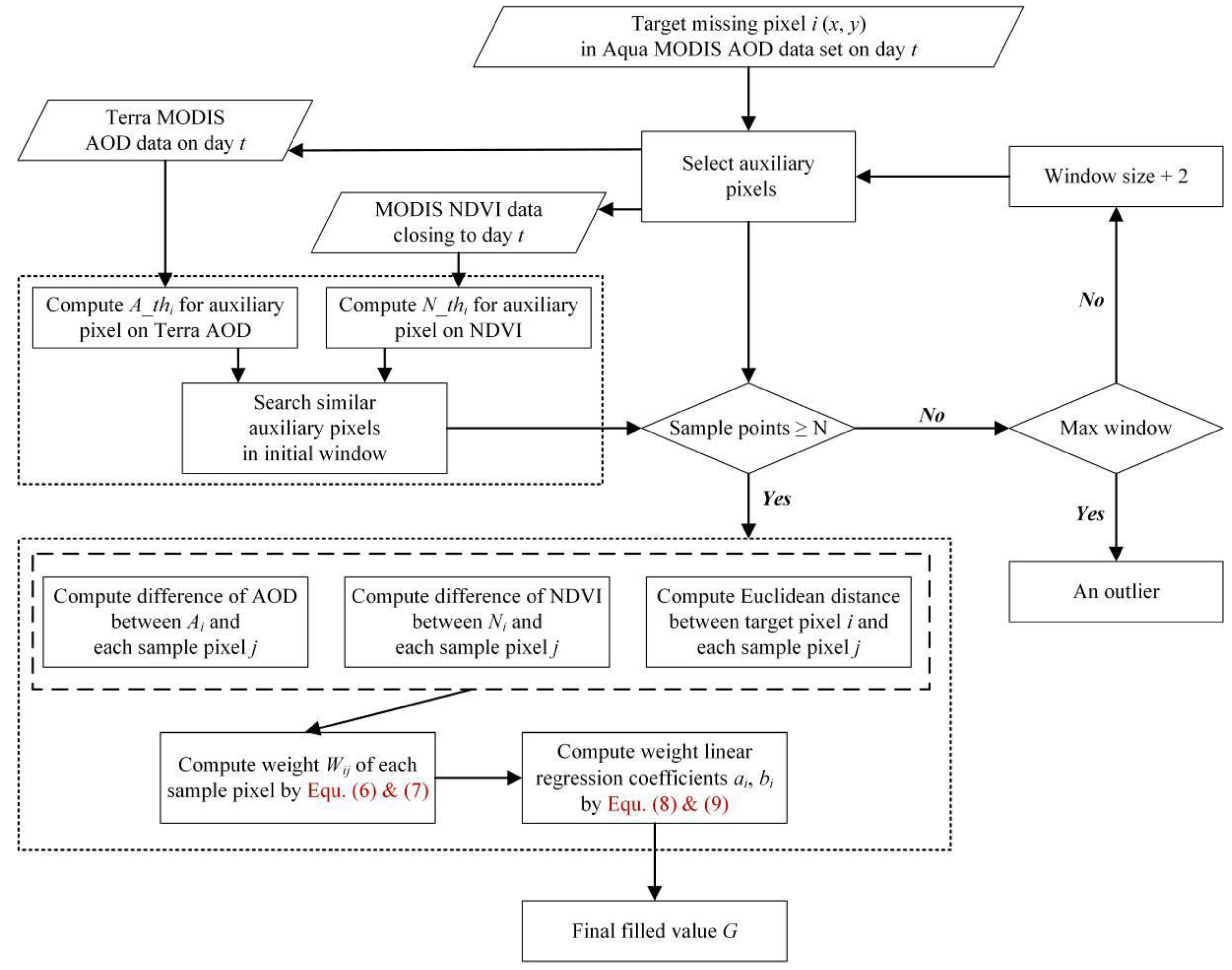
In this study, a linear relationship calculated from locally similar pixels was used to recover each missing pixel from the corresponding auxiliary pixel, where the similar pixels here mean the pixel both having similar AOD and NDVI values. This linear relationship can be expressed as:
where Gi and Ai represent gap-filled pixels in the primary dataset and reference pixels in the auxiliary dataset, respectively, on the target position i, and a and b are the regression coefficients. Accordingly, an adaptive determination procedure is adopted to search for similarity pixels, where the j-th similar pixel must satisfy the following inequality:
where Aj and Ai are the AOD values of the similar pixel and target pixel in the auxiliary AOD datasets, while NDVIj and NDVIi are the NDVI values of position j and target position i in the corresponding NDVI datasets. It is appropriate to determine the AOD similarity and NDVI similarity based on a flexible qualification. Therefore, A_thi and N_thi are set as adaptive thresholds, determined by the local standard variation of AOD and NDVI, respectively:
where μ and μ’ are averages calculated by local 5-pixel by 5-pixel windows in the auxiliary dataset and corresponding NDVI dataset, respectively. The n is the number of pixels in the local 5-pixel by 5-pixel window, which is included in the calculation for threshold. Based on the assumption above, A_thi and N_thi, which respectively represent the AOD threshold in position i and NDVI threshold in positioni, indicate the extent of variation in a local area. The requirements of Equations (2)–(5) ensure that the selection of similar pixels is reasonable in different regions.
After determining the similarity qualification, the selection process was conducted in an initial window centred on the target position. The minimum requirement of the number of selected similar pixels was set as N, in order to guarantee the effectiveness of the following WLR algorithm. If the number of selected similar pixels cannot reach the minimum value, N, the size of the selection window will be enlarged by two pixels. Considering that an oversized selection window will not only consume computing time, but also cause the loss of geospatial relevance, a maximum window size was set. The initial window size and maximum window size were set as 7 and 99, respectively, and the minimum sample points, N, was empirically set to 10 based on the condition of AOD coverage, according to our previous study in WLR [29].
Generally, the least-square approach was employed to estimate the coefficients in Equation (1) from selected similar pixels. However, it is reasonable that each pixel had different contributions according to the similarity of the AOD value, spatial proximity by target position, and the similarity of NDVI. Other than the original WLR algorithm, the NDVI differences were also included in the weight calculation. In this study, at lower NDVI differences, lower differences in AOD values in reference datasets, and a closer distance between the similar and reference pixels, led to a larger weight. These differences were expressed from the following equation:
where NDVIj and Aj represent the NDVI value and AOD value of the reference dataset, respectively, on the j-th similar pixel’s position. NDVIi and Ai represent the NDVI value and AOD value of the auxiliary dataset, respectively, on the target position i. The xj, yj, and xi, yi represent the grid coordinates of the similar and target pixels, and α, β are small values preventing Dij from equaling zero. These small values are set to be the exact half of the minimum scale division, with the alpha chosen to be 0.00005 and the beta chosen to be 0.0005. Therefore, the term characterizes the AOD difference between the corresponding similar pixel and the target pixel in the auxiliary AOD dataset, characterizes the NDVI difference, and describes spatial proximity. Accordingly, the weight of each similar pixel could be normalized using the inversed differences Dij in Equation (7), where the value of Wij ranges from 0 to 1, and the sum of all similar pixels’ weights equals 1.
The calculation of coefficients ai and bi was then performed by adopting the expanded weighted least-squares method [41]:
and
where and are the average of all similar pixels in the selection window in the primary and auxiliary AOD datasets, respectively. The complete flowchart of the NDVI-based WLR AOD recovery method is illustrated in Figure 2.
4. Experimental Results and Analysis
4.1. Simulated Experiment
The objective of this study was to recover the missing pixels in Aqua AOD datasets caused by clouds and typical gaps between MODIS orbit-scanning swaths [17,42].
4.1.1. Recovery Experiment from Orbit Gaps
Simulated masks of the scanning gap were created to conduct simulated experiments on normal Aqua AOD from 2013 to 2015, evaluating the performances of recovery directly.
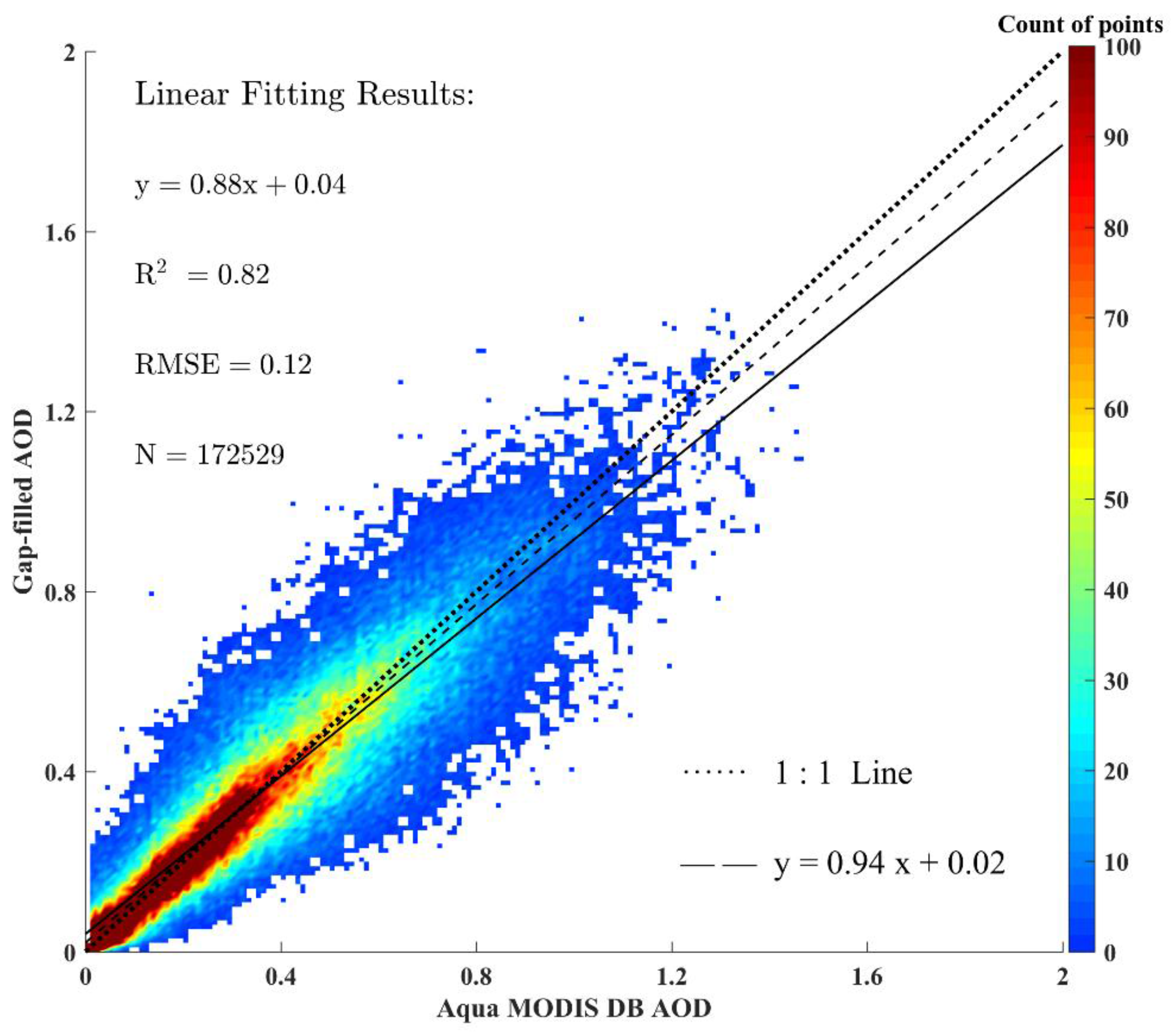
The scanning gaps on the same location appear exactly every 16 days, consistent with the Aqua satellite orbital period. This study utilized one of these gaps over South Asia as a simulated mask and then applied it to the selected Aqua AOD datasets in the other fifteen days with good coverage to obtain the simulated degraded data. Figure 3 illustrates an example of the simulated process. In this simulated condition, 127 groups of degraded Aqua AOD were created from 2013 to 2015. The NWLR was sequentially employed to recover these degraded Aqua AODs using the corresponding Terra AODs on the same day, combined with the corresponding NDVI information. The NWLR performances on the recovery of the gap in South Asia could be evaluated by comparison between the original Aqua AOD and gap-filled AOD, as shown in Figure 4. The scatterplot and linear regression between the original AOD and recovered AOD could directly prove the effectiveness of recovery.
Figure 4 shows the scatterplot of the relationships between the original Aqua AOD (actual value) and the gap-filled AOD (recovered value), where the colour bar represents the density of points. The total fitting pixel pairs reached 172,529, while it should be noted that only the simulated missing pixels participated in the calculation. The fitting results demonstrated that the fitted line was close to the 1:1 line with the decision coefficient, R2, reaching 0.82 and the root mean square error (RMSE) was as low as 0.12. In general, the gap-filled AOD tended to overestimate when the original AOD was lower than 0.3 and tended to underestimate when the original AOD was higher than 0.4, according to the linear fitting equation. In order to avoid the influence of high AOD pairs to the slope and intercept of the linear fit, the dashed line is linearly fitted under the condition that the AOD is smaller than 0.7. As a result, the slope increases from 0.88 to 0.94 which is closer to 1, while the intercept decreases from 0.04 to 0.02 which is closer to 0. Therefore, it is proven that the performance of recovery will be affected by large AOD, which tends to be underestimated.
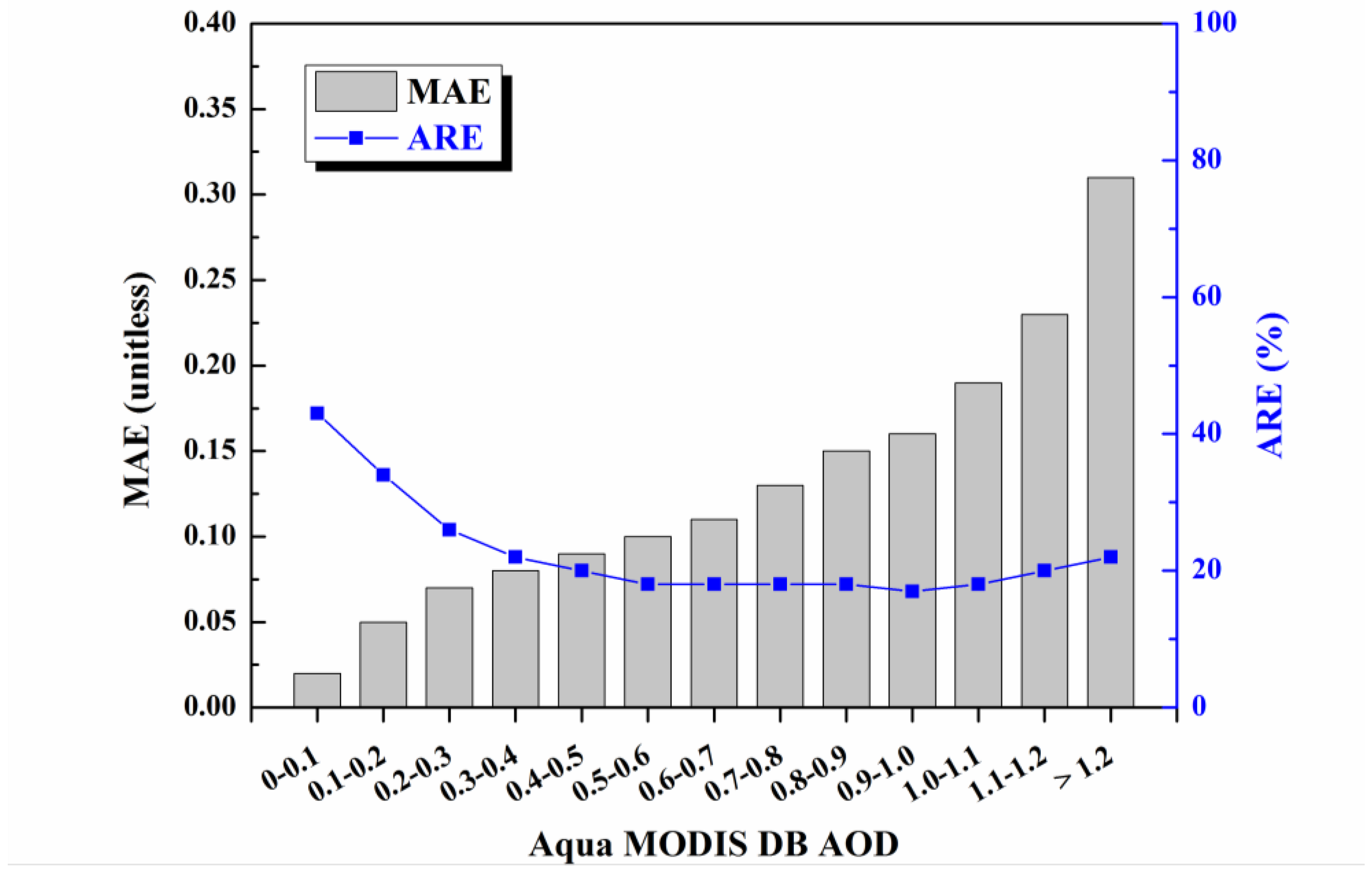
Moreover, a quantitative assessment was conducted to accurately evaluate the errors introduced by the NWLR process along with the variation in the original Aqua AOD. The first metric adopted was the mean absolute error (MAE), which had advantages over RMSE in assessing average model performance, such as measuring the degree of bias [43]. It is defined in Equation (10):
where N is the total number of gap-filled pixels, and Gi and Oi are the ith gap-filled AOD and corresponding original AOD values, respectively. The second index adopted was the average relative error (ARE), which could measure the error range based on the original AOD. It is defined in Equation (11):
The lower MAE and ARE indicate a better performance of AOD recovery. As shown in Figure 5, although the MAE increased with the increase of the original AOD, the ARE maintained a value of approximately 20% when the original AOD was beyond 0.4. This result is in agreement with the hypothesis of a linear relationship between the multi-temporal AOD, because the absolute error would proportionately increase along with the growth of the original AOD.
4.1.2. Recovery Experiment from Cloud Obscuration
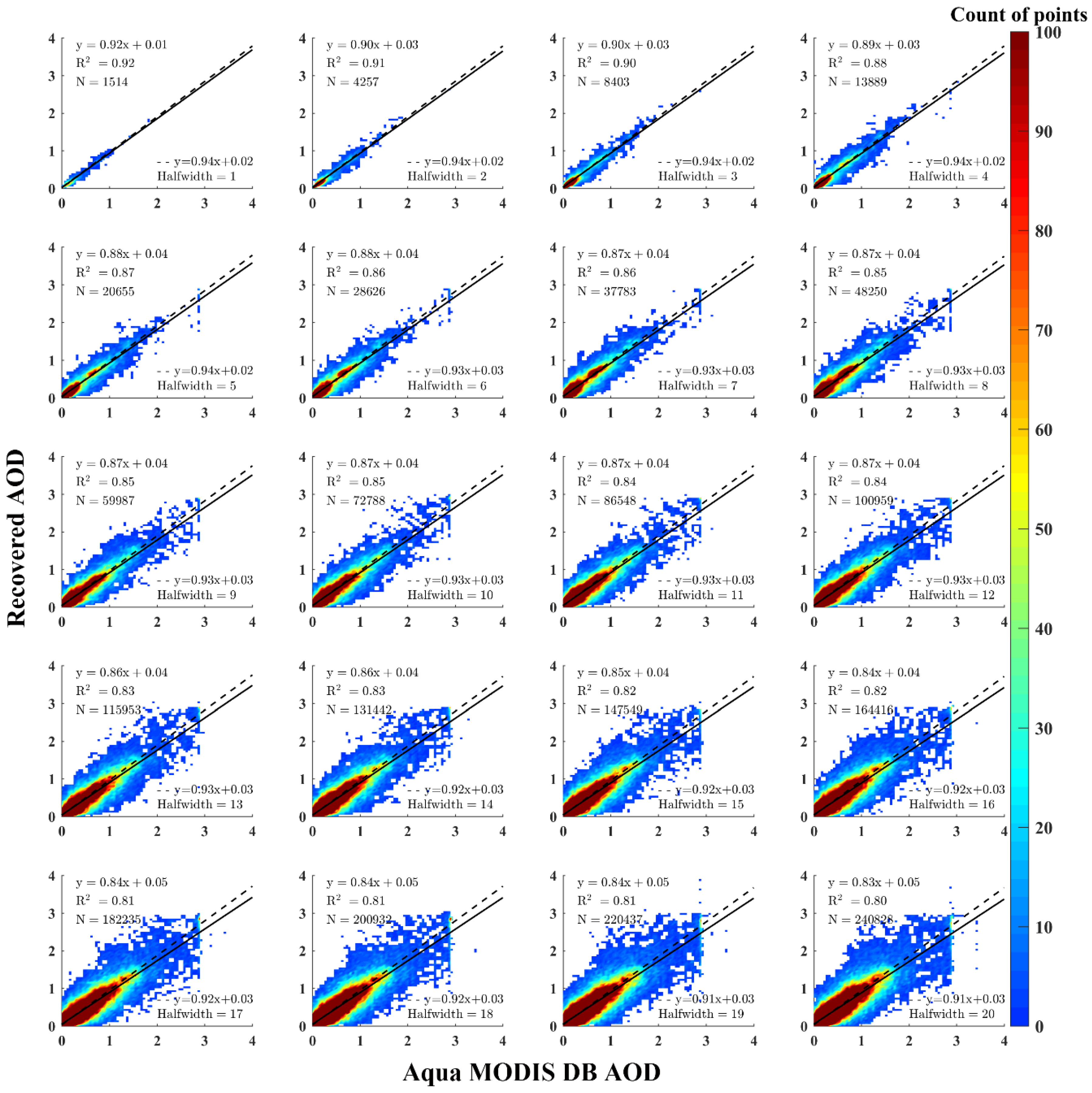
Similar simulated experiments have been conducted in the mega city of Beijing. This simulated experiment aimed at simulating missing pixels caused by cloud obscuration. Because the size and appearance of a cloud cannot be determined in advance, window masks of different sizes, centred on the AERONET station of Beijing (116.381°E, 39.977°N), were created. The size of the window mask was designed ranging from 3 to 41 pixels, with the interval set as 2 pixels, and the half width ranged from 1 to 20 pixels. Similar to the gap-filled experiments above, window masks of different sizes were applied to the selected Aqua AOD datasets with good coverage in Beijing to obtain simulated degraded data. In this premise, 181 groups of degraded Aqua AOD were created from 2013 to 2015, and each group performed a simulated window mask exactly twenty times. The corresponding Terra AOD was then utilized to recover the simulated missing pixels in Aqua AOD using NWLR, combined with the corresponding NDVI dataset. The performance on the recovery of AOD in Beijing was evaluated by comparison between the original Aqua AOD and recovered AOD, which is shown in Figure 6, as well as the sensitivity test for window mask size.
Scatterplots between the original Aqua AOD and recovered AOD are illustrated in Figure 6, where these twenty scatterplots sequentially correspond to the window mask half width ranging from 1 to 20. The colour bar displays the density of points and the lines represent the results of linear fitting. Along with the increase in the simulated window mask, the slope of the linear fitting equation decreased from 0.92 to 0.83, the intercept of the linear fitting equation increased from 0.01 to 0.05, and the linear regression R2 declined from 0.92 to 0.80. It can be concluded that when the window mask was smallest, the optimal recovery performances were achieved, and the effectiveness of recovery decreased as the window mask became larger. When the half width of the window mask was 1, the fitting line was closest to the 1:1 actual line, with the decision coefficient of the linear regression R2 reaching 0.92. While the half width of the window mask was 20, the decision coefficient R2 of linear fitting was still over 0.8. In addition, it should not be ignored that there was an obvious underestimation when original AOD value was relatively high, no matter the size of the window designed. In order to eliminate the effect of high AOD pairs to the slope and intercept of the linear fit, the linear fitting under the condition that the AOD is smaller than 0.7 has been conducted in each sub-figure via dashed line. As a result, the slope increases to be closer to 1 and the intercept decreases to be closer to 0, which indicates that the performance of recovery will be affected by a large AOD in each size of the cloud mask. It indicated that the extent of underestimation was aggravated as the window mask and AOD range became larger. From a practical perspective, this type of underestimation in Beijing might cause a negative bias in overall aerosol assessments. Nevertheless, it was meaningful that if there had been approximately 400 km 400 km missing data from the Aqua AOD caused by a mono-temporal cloud obscuration, over 80% of the recovered AOD by NWLR using Terra AOD was consistent with the real AOD.
The MAE and ARE metrics were similarly adopted to evaluate errors introduced by the NWLR process along with a variation in the original Aqua AOD in Beijing. As demonstrated in Figure 7, the MAE increased with the growth of original AOD, and the ARE remained around 20% when the original AOD was above 0.6. This result was similar with those obtained in gap-filled simulated experiments, even in the condition that the AOD values in Beijing were quite different from the AOD values in South Asia, which indicated that the ARE from the recovered AOD using the proposed NWLR tended toward stability (~20%) when the original AOD value was no longer relatively small.
4.2. Overall Recovering Performances
The NWRL algorithm were applied to the whole domain and this section discusses the combined effect of gap and cloud obscuration recovery as a whole. Similar to the simulated experiments above, the gaps would not present above 28°N, while cloud obscuration might appear at every possible position in the whole domain.
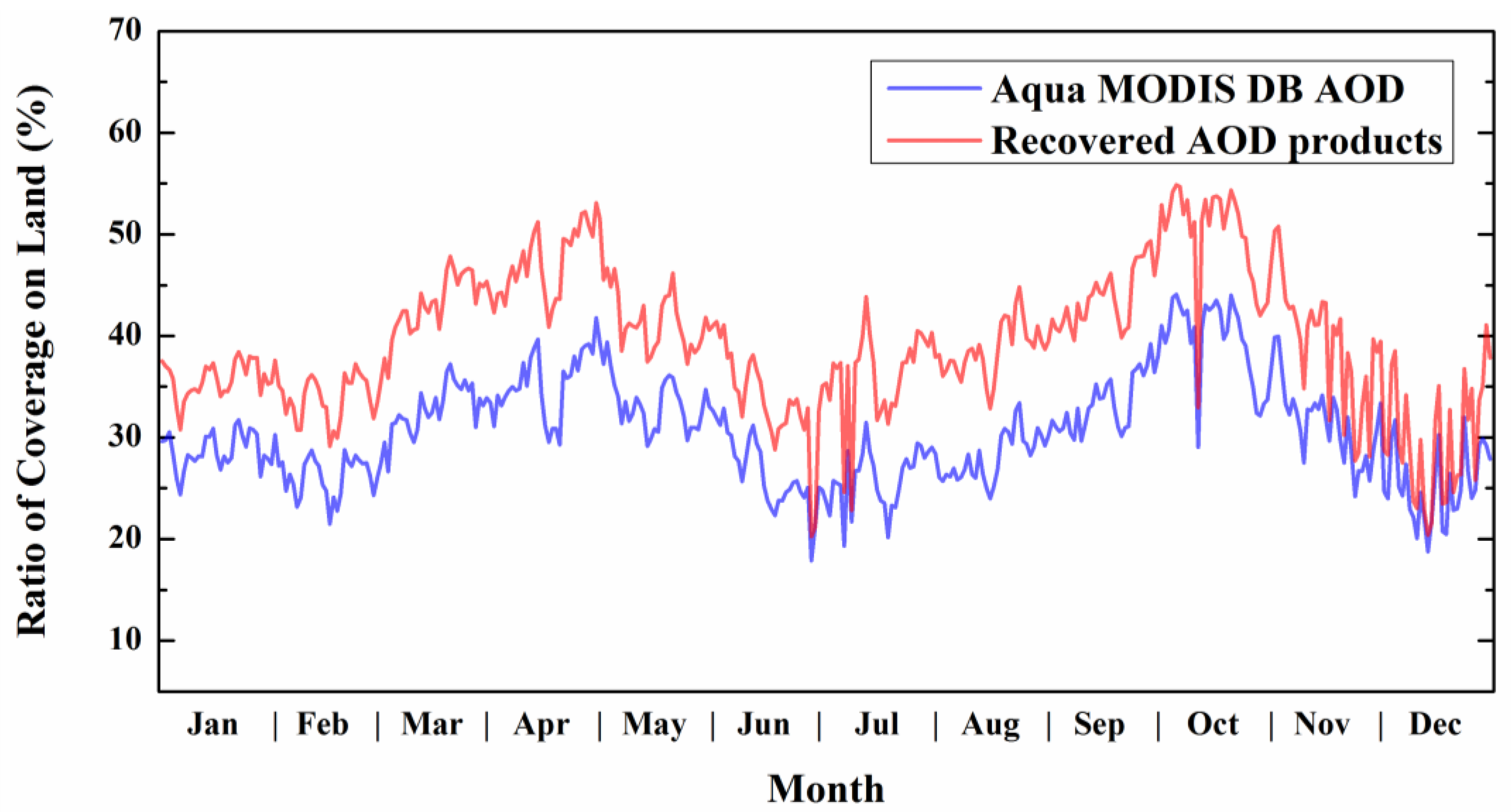
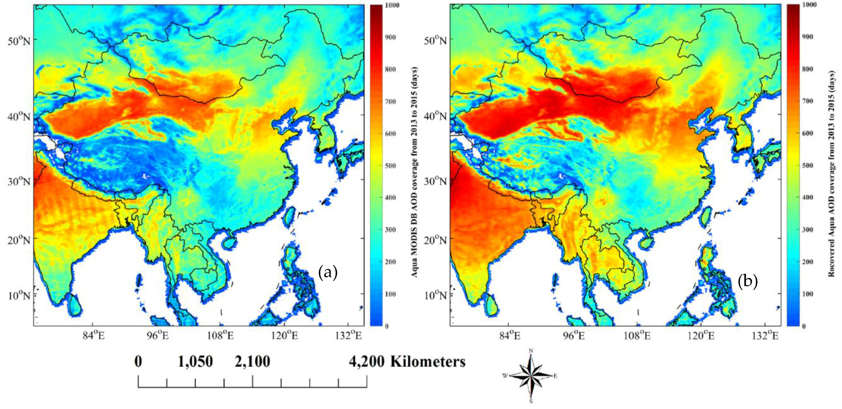
The averaged ratio of valid AOD coverage over land for Aqua MODIS DB and recovered AOD from 2013 to 2015 is shown in Figure 8, which demonstrates an improvement in coverage all year around. In general, the mean improvement from Aqua AOD to recovered AOD was approximately an additional 10% of land AOD coverage. The primary trend illustrated that the coverage in spring and autumn was higher than the coverage in summer and winter, which was caused by the summer monsoon and snow-cover in winter, respectively. Furthermore, the spatial distribution of the total coverage-days from 2013 to 2015 was compared between the Aqua AOD and recovered AOD in Figure 9, and different improvement occurred in different regions. The coverage was improved in Southwest Asia (approximately from 10°N to 25°N), the Southeast coast (cantered at ~25°N, 115°E), and central China (cantered at ~30°N, 110°E) to a certain extent, while it apparently improved in North China (cantered at ~40°N, 115°E) and Mongolia (cantered at ~45°N, 100°E). In addition, obvious improvement was made in regions of South Asia, where the MODIS orbit scanning gaps were effectively recovered.
5. Accuracy Evaluation and Discussion
It is widely acknowledged that there are errors between satellite-derived AOD values and actual AOD values. Meanwhile, recovered AOD using NWLR would inevitably introduce differences compared to the original satellite-derived AOD. Thus, it is necessary to discuss whether the errors between recovered AOD and actual AOD expand from the satellite-derived AOD errors. As stated above, the AOD measured by AERONET is generally considered as an actual value for the validation of AOD products. The 56 AERONET sites were included in the validation with only level 2.0 AOD products used.
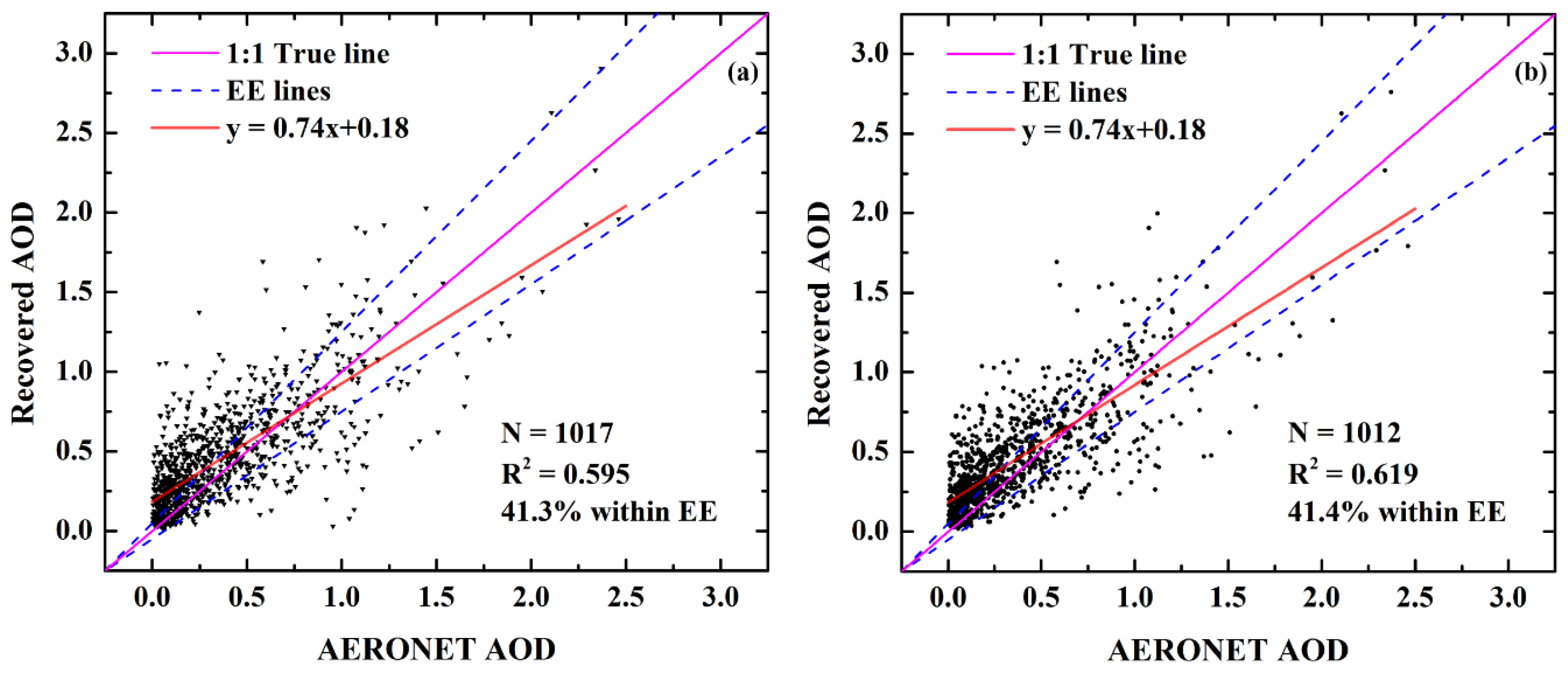
Figure 10 shows the scatterplot between the recovered AOD and corresponding AERONET AOD in the conditions that the Aqua MODIS DB AOD failed to retrieve a valid value on one specific pixel, where this pixel could have been recovered by Terra MODIS DB AOD, and the AERONET site on this pixel obtained a valid level 2.0 AOD around 1:30 p.m. local time. In Figure 10a, the AOD gridded pixel with its centre closest to the ground AERONET site was extracted, while the ground AERONET site that corresponds to the aggregation of 3 × 3 pixels is illustrated in Figure 10b. Under this screening condition, 1017 pairs and 1012 pairs of AOD were extracted from 2013 to 2015, respectively, in single pixel and aggregated pixel. The linear regression between AERONET AOD and recovered AOD achieved an R2 of approximately 0.60 and a correlation coefficient over 0.77, which performed similarly to previous approaches, the R2 reaching 0.59 in the United States and achieving 0.56 in parts of East Asia, respectively [18,26]. It showed that the NWLR method had an advantage in AOD recovery in the whole East and South Asia regions to a certain extent. Over 41% of AODs fell within the reference expected error (EE) envelope (the scope equations are defined as [17]), which met the requirement for application. Furthermore, in a previous evaluation of the whole China region, it has been shown that there are great differences in validation between AERONET AOD and MODIS DB AOD, with all quality assurances, due to their different locations, with the slope of the linear regression equation varying from 0.67 to 1.21 and R2 ranging from 0.20 to 0.85 [32]. Therefore, the overall accuracy of the validation between AERONET AOD and recovered AOD would significantly decline, since it neglected the different accuracies in original MODIS DB AOD retrievals from different regions. A further experiment was accordingly performed on the simulated experiments above, which discussed the validation between the retrieved AOD and AERONET AOD in South Asia and Beijing, respectively.
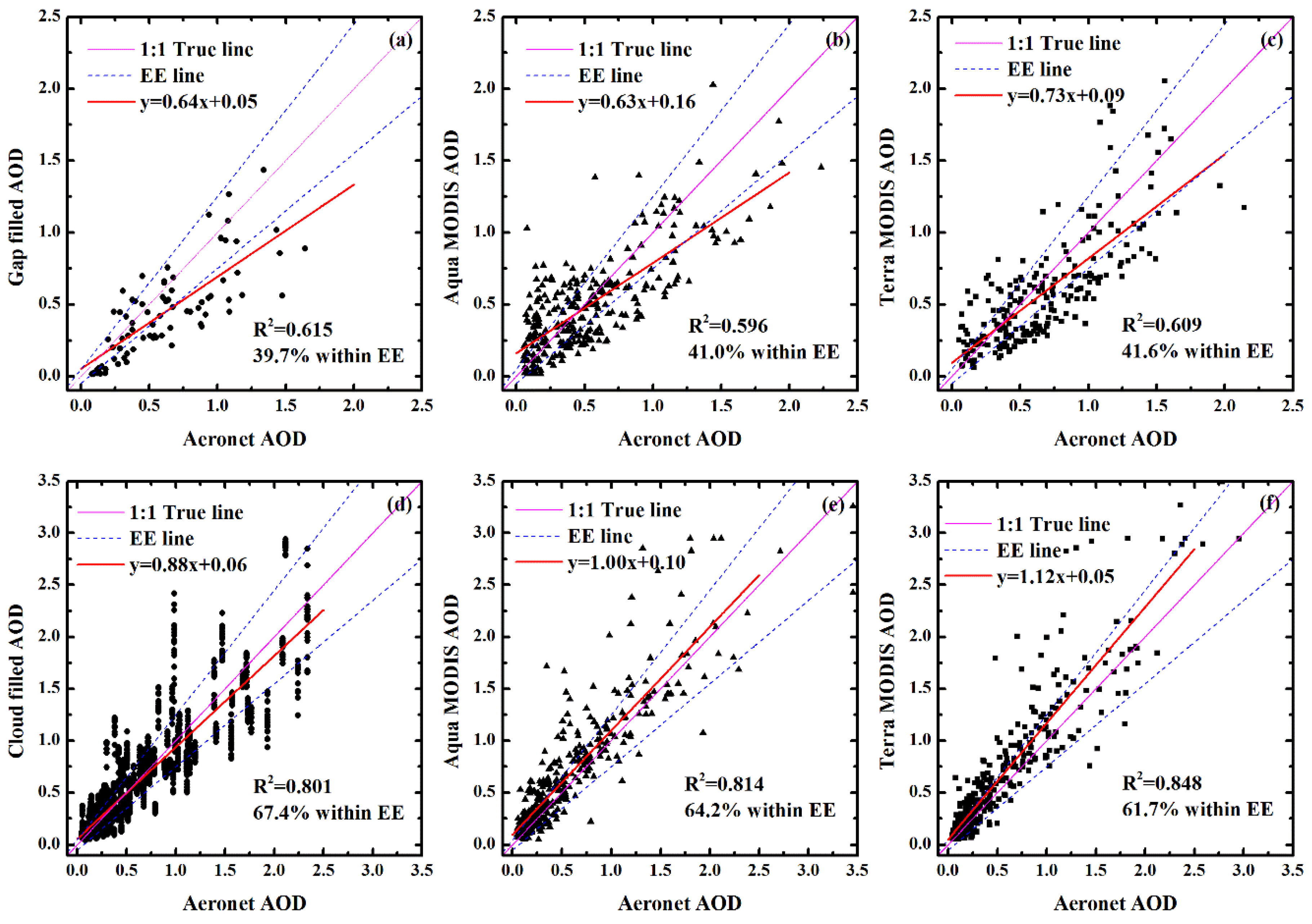
There were two selected AERONET stations in the simulated gap mask in South Asia, namely Nong_Khai and Luang_Namtha, and the centre of the simulated window mask was the Beijing AERONET site. The validation was conducted between the AERONET AOD against the gap-filled AOD/recovered AOD, original Aqua MODIS DB AOD, and referenced Terra MODIS DB AOD. As shown in Figure 11a–c, although only around 39.7% of recovered AODs fell within the EE envelope, with the slope of the linear regression at just 0.64, both the original AOD and referenced AOD had similar validated accuracy against the AERONET AOD, with 41.0% and 41.6% of AODs falling within the EE envelope, respectively. The similar phenomenon appeared in the validation in Beijing where the accuracy of the recovered AOD was close to the original and referenced AOD in Figure 11d–f. The behaviour was quite different between Southeast Asia and the Beijing area, which could be explained by the different accuracy between the satellite-derived AOD and AERONET AOD, because the recovered AOD was completely determined by the original Aqua and Terra AOD datasets. Therefore, NWLR AOD recovered errors do not expand from the satellite-derived AOD errors, and the accuracy of recovered AOD had an ideal consistency with the accuracy of the original Aqua MODIS DB AOD when validating against the AERONET AOD.
6. Conclusions
As MODIS AOD clearly lacks coverage from the orbit-scanning gap and cloud obscuration, the NWLR method is proposed to synthetically describe the factors influencing the relationship between Terra MODIS AOD and Aqua MODIS AOD, with the goal of AOD recovery rather than mathematical AOD fusion. The similarity of AOD, the Euclidean distance, and the similarity of NDVI are defined as influencing factors on the temporal relationship, which will further affect the weight in regression.
Simulated experiments were conducted from 2013 to 2015 in South Asia and Beijing, to evaluate the performances of recovery on the orbit-scanning gap and cloud obscuration conditions, respectively. Both experiments applied simulated masks to the Aqua AOD datasets, and the NWLR was sequentially employed to recover these degraded Aqua AOD using the corresponding Terra AOD on the same day, combining the corresponding NDVI information. The evaluation of recovered AOD against original Aqua AOD demonstrated that the decision coefficient R2 between them reached up to 0.8 with an absolute relative error staying at approximately 20% with the increase of original AOD values, which suggested that the NWLR method performed well in recovery. Moreover, the AERONET AOD from 56 sites in East and South Asia was utilized to validate the accuracy of the recovered AOD, where over 41% of the recovered AODs fell within the EE envelope, meeting the requirements for application. Additional validation conducted in South Asia and Beijing showed that the recovery by NWLR did not expand the satellite-derived AOD errors, and the accuracy of the recovered AOD was consistent with the accuracy of the original Aqua MODIS DB AOD when validating against the AERONET AOD.
Furthermore, the recovery results illustrated that approximately a 10% improvement in coverage was brought by NWLR, and there were obvious improvements in coverage over North China, Mongolia, and South Asia. This approach could be generalized for use by other satellites in similar multi-temporal recovery, which could further include AOD retrieval errors by different satellites, and could apply nonlinear multi-temporal regression. This study had limitations from snow cover or daylong cloud obscuration, and our future studies will focus on the quantitative description of the multi-temporal relationship, and will consider assigning different weights to AOD differences and NDVI differences based on their quantitative effect on the AOD retrieval, for instance, combined with the inconsistency of different AOD products. The Aqua MODIS DB AOD with better spatial coverage and recovery accuracy could provide better support in aerosol spatio-temporal analysis, assessment of the atmospheric environment, and aerosol data assimilation.
Acknowledgments
This research was supported by the National Natural Science Foundation of China (No. 41601044, No. 41101334, No. 41127901, and No. 41571344), the Hubei Provincial Natural Science Foundation of China (No. 2016CFB620, and No. 2015CFA002), the Special Fund for Basic Scientific Research of Central Colleges, China University of Geosciences, Wuhan (No. CUG15063), and China Postdoctoral Science Foundation (No. 2015M572198). All authors gratefully thank AERONET PIs and related staff for their efforts in maintaining measurement sites.
Author Contributions
The research topic was designed by Tianhao Zhang and Zhongmin Zhu. Tianhao Zhang, Lunche Wang, Chao Zeng, and Zerun Zhu conducted the experiment, and the paper was written by Tianhao Zhang. Wei Gong, Kun Sun, and Huanfeng Shen checked the experimental data and examined the experimental results. All authors agreed to the submission of the manuscript.
Conflicts of Interest
The authors declare no conflict of interest.
References
- Kaufman, Y.J.; Tanré, D.; Boucher, O. A satellite view of aerosols in the climate system. Nature 2002, 419, 215–223. [Google Scholar] [CrossRef] [PubMed]
- Xia, X. A critical assessment of direct radiative effects of different aerosol types on surface global radiation and its components. J. Quant. Spectrosc. Radiat. Transf. 2014, 149, 72–80. [Google Scholar] [CrossRef]
- Stocker, T.F.; Qin, D.; Plattner, G.K.; Tignor, M.; Allen, S.K.; Boschung, J.; Nauels, A.; Xia, Y.; Bex, V.; Midgley, P.M. The Physical Science Basis. Contribution of Working Group I to the Fifth Assessment Report of the Intergovernmental Panel on Climate Change; Cambridge University Press: Cambridge, UK, 2013. [Google Scholar]
- Dubovik, O.; Smirnov, A.; Holben, B.N.; King, M.D.; Kaufman, Y.J.; Eck, T.F.; Slutsker, I. Accuracy assessments of aerosol optical properties retrieved from aerosol robotic network (AERONET) sun and sky radiance measurements. J. Geophys. Res. Atmos. 2000, 105, 9791–9806. [Google Scholar] [CrossRef]
- Wang, L.; Gong, W.; Singh, R.P.; Xia, X.; Che, H.; Zhang, M.; Lin, H. Aerosol optical properties over mount song, a rural site in Central China. Aerosol Air Qual. Res. 2015, 15. [Google Scholar] [CrossRef]
- Che, H.; Zhang, X.Y.; Xia, X.; Goloub, P.; Holben, B.; Zhao, H.; Wang, Y.; Zhang, X.C.; Wang, H.; Blarel, L. Ground-based aerosol climatology of china: Aerosol optical depths from the China aerosol remote sensing network (CARSNET) 2002–2013. Atmos. Chem. Phys. 2015, 15, 7619–7652. [Google Scholar] [CrossRef]
- Pan, L.; Che, H.; Geng, F.; Xia, X.; Wang, Y.; Zhu, C.; Chen, M.; Gao, W.; Guo, J. Aerosol optical properties based on ground measurements over the Chinese Yangtze delta region. Atmos. Environ. 2010, 44, 2587–2596. [Google Scholar] [CrossRef]
- Chatterjee, A.; Michalak, A.M.; Kahn, R.A.; Paradise, S.R.; Braverman, A.J.; Miller, C.E. A geostatistical data fusion technique for merging remote sensing and ground-based observations of aerosol optical thickness. J. Geophys. Res. Atmos. 2010. [Google Scholar] [CrossRef]
- Anderson, T.L.; Charlson, R.J.; Bellouin, N.; Boucher, O.; Chin, M.; Christopher, S.A.; Haywood, J.; Kaufman, Y.J.; Kinne, S.; Ogren, J.A. An “a-train” strategy for quantifying direct climate forcing by anthropogenic aerosols. Bull. Am. Meteorol. Soc. 2005, 86, 1795. [Google Scholar] [CrossRef]
- Kim, S.W.; Yoon, S.C.; Kim, J.; Kim, S.Y. Seasonal and monthly variations of columnar aerosol optical properties over east asia determined from multi-year MODIS, LIDAR, and aeronet sun/sky radiometer measurements. Atmos. Environ. 2007, 41, 1634–1651. [Google Scholar] [CrossRef]
- Ma, Z.; Hu, X.; Sayer, A.M.; Levy, R.; Zhang, Q.; Xue, Y.; Tong, S.; Bi, J.; Huang, L.; Liu, Y. Satellite-based spatiotemporal trends in PM2.5 concentrations: China, 2004–2013. Environ. Health Perspect. 2016, 124, 184–192. [Google Scholar] [CrossRef] [PubMed]
- Chu, D.A.; Kaufman, Y.J.; Ichoku, C.; Remer, L.A.; Tanré, D.; Holben, B.N. Validation of MODIS aerosol optical depth retrieval over land. Geophys. Res. Lett. 2002, 29, 8007. [Google Scholar] [CrossRef]
- Engel-Cox, J.A.; Hoff, R.M. Qualitative and quantitative evaluation of MODIS satellite sensor data for regional and urban scale air quality. Atmos. Environ. 2004, 38, 2495–2509. [Google Scholar] [CrossRef]
- Mi, W.; Li, Z.; Xia, X.; Holben, B.; Levy, R.; Zhao, F.; Chen, H.; Cribb, M. Evaluation of the moderate resolution imaging spectroradiometer aerosol products at two aerosol robotic network stations in China. J. Geophys. Res. Atmos. 2007, 112, 321–341. [Google Scholar] [CrossRef]
- Sayer, A.M.; Hsu, N.C.; Bettenhausen, C.; Jeong, M.J. Validation and uncertainty estimates for MODIS collection 6 “deep blue” aerosol data. J. Geophys. Res. Atmos. 2013, 118, 7864–7872. [Google Scholar] [CrossRef]
- Sayer, A.M.; Munchak, L.A.; Hsu, N.C.; Levy, R.C.; Bettenhausen, C.; Jeong, M.J. MODIS collection 6 aerosol products: Comparison between aqua’s e-deep blue, dark target, and “merged” data sets, and usage recommendations. J. Geophys. Res. Atmos. 2015. [Google Scholar] [CrossRef]
- Hsu, N.C.; Jeong, M.J.; Bettenhausen, C.; Sayer, A.M.; Hansell, R.; Seftor, C.S.; Huang, J.; Tsay, S.C. Enhanced deep blue aerosol retrieval algorithm: The second generation. J. Geophys. Res. Atmos. 2013, 118, 9296–9315. [Google Scholar] [CrossRef]
- Tang, Q.; Bo, Y.; Zhu, Y. Spatiotemporal fusion of multiple-satellite aerosol optical depth (AOD) products using bayesian maximum entropy method. J. Geophys. Res. Atmos. 2016. [Google Scholar] [CrossRef]
- Leeuw, G.D.; Holzer-Popp, T.; Bevan, S.; Davies, W.H.; Descloitres, J.; Grainger, R.G.; Griesfeller, J.; Heckel, A.; Kinne, S.; Klüser, L. Evaluation of seven european aerosol optical depth retrieval algorithms for climate analysis. Remote Sens. Environ. 2015, 162, 295–315. [Google Scholar] [CrossRef]
- Peng, X.; Shen, H.; Zhang, L.; Zeng, C.; Yang, G.; He, Z. Spatially continuous mapping of daily global ozone distribution (2004–2014) with the Aura Omi sensor. J. Geophys. Res. Atmos. 2016. [Google Scholar] [CrossRef]
- Liu, H.; Pinker, R.T.; Holben, B.N. A global view of aerosols from merged transport models, satellite, and ground observations. J. Geophys. Res. Atmos. 2005. [Google Scholar] [CrossRef]
- Mélin, F.; Zibordi, G.; Djavidnia, S. Development and validation of a technique for merging satellite derived aerosol optical depth from Seawifs and MODIS. Remote Sens. Environ. 2007, 108, 436–450. [Google Scholar] [CrossRef]
- Xue, Y.; Xu, H.; Mei, L.; Guang, J.; Guo, J.; Li, Y.; Hou, T.; Li, C.; Yang, L.; He, X. Merging aerosol optical depth data from multiple satellite missions to view agricultural biomass burning in Central and East China. Atmos. Chem. Phys. 2012, 12, 10461–10492. [Google Scholar] [CrossRef]
- Guo, J.; Gu, X.; Yu, T.; Cheng, T.; Chen, H.; Xie, D. Trend analysis of the aerosol optical depth over China using fusion of MODIS and MISR aerosol products via adaptive weighted estimate algorithm. Proc. SPIE 2013. [Google Scholar] [CrossRef]
- Nguyen, H.; Cressie, N.; Braverman, A. Spatial statistical data fusion for remote sensing applications. J. Am. Stat. Assoc. 2012, 107, 1004–1018. [Google Scholar] [CrossRef]
- Puttaswamy, S.J.; Hai, M.N.; Braverman, A.; Hu, X.; Liu, Y. Statistical data fusion of multi-sensor AOD over the continental United States. Geocarto Int. 2014, 29, 48–64. [Google Scholar] [CrossRef]
- Sayer, A.M.; Hsu, N.C.; Bettenhausen, C.; Jeong, M.J. Global and regional evaluation of over-land spectral aerosol optical depth retrievals from Seawifs. Atmos. Measu. Tech. 2012, 5, 2169–2220. [Google Scholar] [CrossRef]
- Vermote, E.F.; Saleous, N.Z.E.; Justice, C.O. Atmospheric correction of MODIS data in the visible to middle infrared: First results. Remote Sens. Environ. 2002, 83, 97–111. [Google Scholar] [CrossRef]
- Zeng, C.; Shen, H.; Zhang, L. Recovering missing pixels for Landsat ETM+ slc-off imagery using multi-temporal regression analysis and a regularization method. Remote Sens. Environ. 2013, 131, 182–194. [Google Scholar] [CrossRef]
- Liu, Z.; Liu, Q.; Lin, H.C.; Schwartz, C.S.; Lee, Y.H.; Wang, T. Three-dimensional variational assimilation of MODIS aerosol optical depth: Implementation and application to a dust storm over East Asia. J. Geophys. Res. Atmos. 2011, 116, 23206. [Google Scholar] [CrossRef]
- Schwartz, C.S. Assimilating aerosol observations with a “hybrid” variational-ensemble data assimilation system. J. Geophys. Res. Atmos. 2014, 119, 4043–4069. [Google Scholar] [CrossRef]
- Tao, M.; Chen, L.; Wang, Z.; Tao, J.; Che, H.; Wang, X.; Wang, Y. Comparison and evaluation of the MODIS collection 6 aerosol data in China. J. Geophys. Res. Atmos. 2015. [Google Scholar] [CrossRef]
- NASA LAADS MODIS. Available online: http://ladsweb.nascom.nasa.gov/ (accessed on 2 April 2017).
- Tucker, C.J. Red and photographic infrared linear combinations for monitoring vegetation. Remote Sens. Environ. 1979, 8, 127–150. [Google Scholar] [CrossRef]
- Tucker, C.J.; Sellers, P.J. Satellite remote sensing of primary production. Int. J. Remote Sens. 1986, 7, 1395–1416. [Google Scholar] [CrossRef]
- Holben, B.N.; Eck, T.F.; Slutsker, I.; Tanr, D.; Buis, J.P.; Setzer, A.; Vermote, E.; Reagan, J.A.; Kaufman, Y.J.; et al. Aeronet—A federated instrument network and data archive for aerosol characterization. Remote Sens. Environ. 1998, 66, 1–16. [Google Scholar] [CrossRef]
- Dubovik, O.; King, M.D. A flexible inversion algorithm for retrieval of aerosol optical properties from sun and sky radiance measurements. J. Geophys. Res. 2000, 105, 20673–20696. [Google Scholar] [CrossRef]
- AERONET AOD. Available online: http://aeronet.gsfc.nasa.gov/ (accessed on 2 April 2017).
- Smirnov, A.; Holben, B.N.; Eck, T.F.; Dubovik, O.; Slutsker, I. Cloud-screening and quality control algorithms for the aeronet database. Remote Sens. Environ. 2000, 73, 337–349. [Google Scholar] [CrossRef]
- Ångström, A. On the atmospheric transmission of sun radiation and on dust in the air. Geograf. Ann. 1929, 11, 156–166. [Google Scholar] [CrossRef]
- Ruppert, D.; Wand, M.P. Multivariate locally weighted least squares regression. Ann. Stat. 1994, 22, 1346–1370. [Google Scholar] [CrossRef]
- Nirala, M. Technical note: Multi-sensor data fusion of aerosol optical thickness. Int. J. Remote Sens. 2008, 29, 2127–2136. [Google Scholar] [CrossRef]
- Willmott, C.J.; Matsuura, K. Advantages of the mean absolute error (MAE) over the root mean square error (RMSE) in assessing average model performance. Clim. Res. 2005, 30, 79. [Google Scholar] [CrossRef]
Figure 1.
Maps of seasonal averaged Aerosol Optical Depth (AOD) in summer (a) and in winter (b), respectively; illustration of 56 Aerosol Robotic Network (AERONET) sites (red solid triangles) in research areas (c); and maps of seasonal averaged Normalized Difference Vegetation Index (NDVI) in summer (d) and in winter (e), respectively.
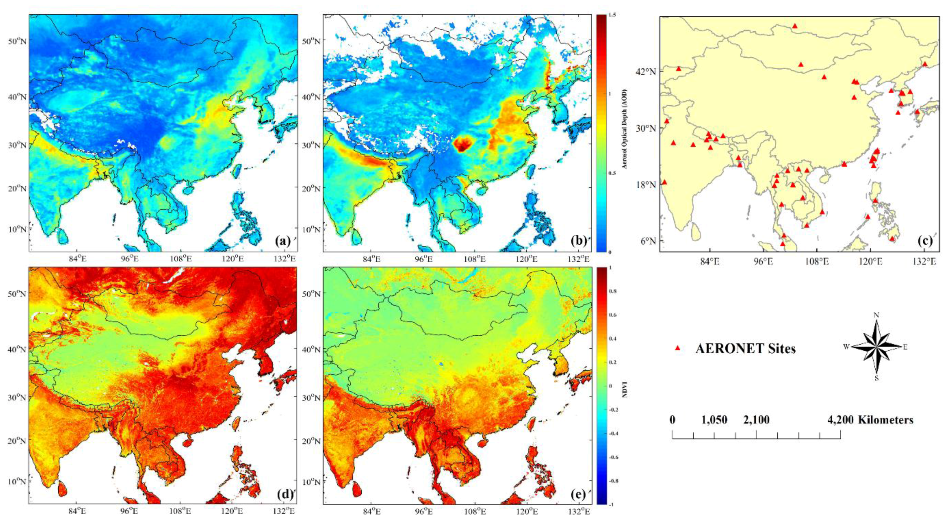
Figure 2.
NDVI-Based Weighted Linear Regression (WLR) algorithm flowchart.

Figure 3.
Simulated mask of Aqua Moderate Resolution Imaging Spectroradiometer (MODIS) scanning gap applied to Aqua MODIS AOD products without the same gap (diagram example on 2 March 2014).
Figure 3.
Simulated mask of Aqua Moderate Resolution Imaging Spectroradiometer (MODIS) scanning gap applied to Aqua MODIS AOD products without the same gap (diagram example on 2 March 2014).

Figure 4.
Scatterplot of the original Aqua MODIS Deep Blue (DB) AOD against the gap-filled AOD values of all simulated mask pixels in South Asia from 2013 to 2015. The solid black line illustrates the fitting line, the dotted black line represents the 1:1 line, and the dashed black line represents the linear fitting equation by limiting AOD smaller than 0.7.

Figure 5.
Trend of mean absolute error (MAE) and average relative error (ARE) based on the division of original AOD values from the simulated gap-filled process in South Asia.
Figure 5.
Trend of mean absolute error (MAE) and average relative error (ARE) based on the division of original AOD values from the simulated gap-filled process in South Asia.

Figure 6.
Scatterplots of the original Aqua MODIS DB AOD against the recovered AOD values of all simulated window mask pixels in Beijing, combined with a sensitivity test on mask window half width, from 2013 to 2015. The black solid lines represent the linear regression results in each figure, and the black dashed lines represent linear fitting by limiting AOD smaller than 0.7. The colour bar in this figure indicates the density of points.

Figure 7.
Trend of mean absolute error (MAE) and average relative error (ARE) based on the division of the original AOD values in the simulated window sensitivity test in Beijing.
Figure 7.
Trend of mean absolute error (MAE) and average relative error (ARE) based on the division of the original AOD values in the simulated window sensitivity test in Beijing.
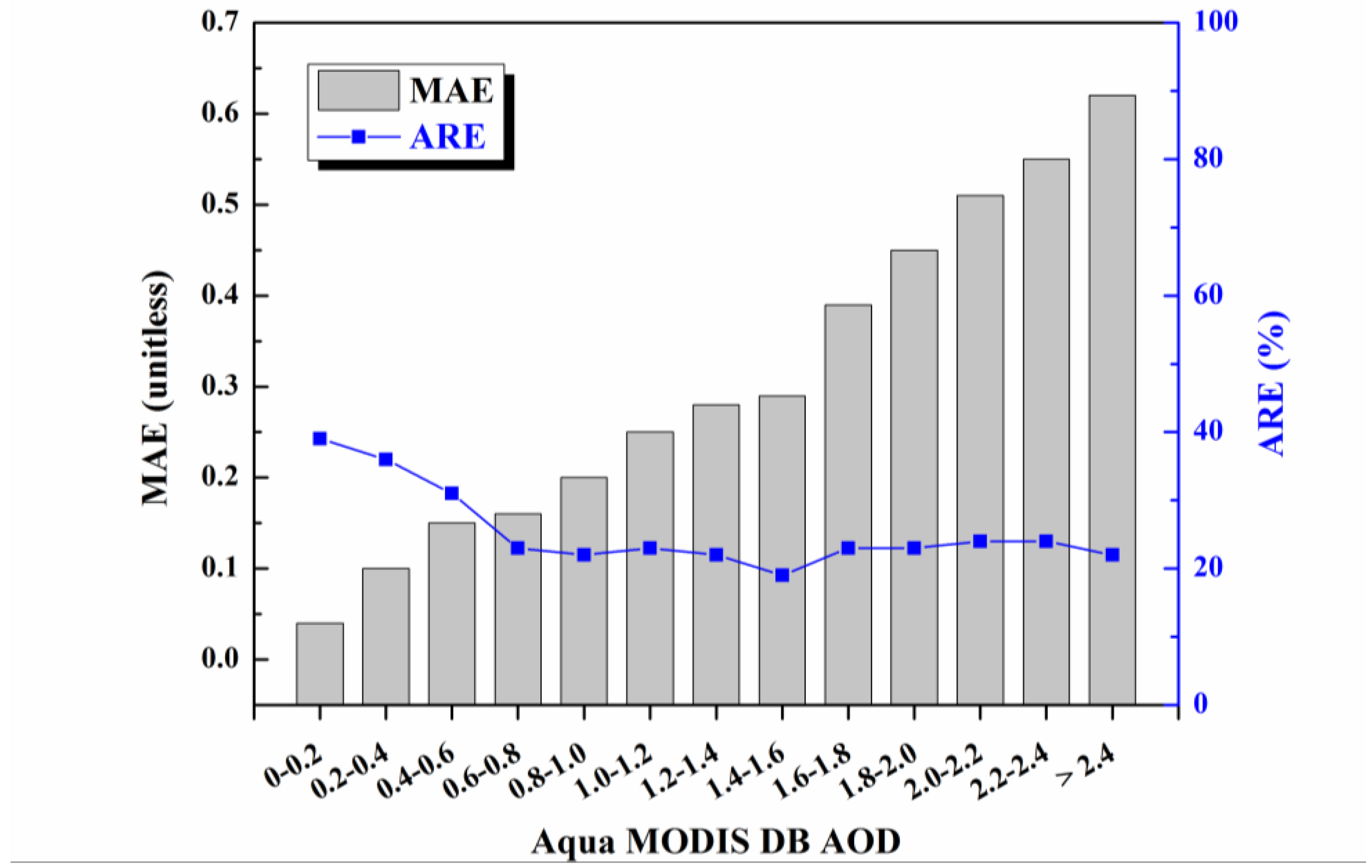
Figure 8.
The averaged ratio of pixels with valid AOD on land for the original Aqua MODIS DB AOD datasets and the recovered AOD products from 2013 to 2015.
Figure 8.
The averaged ratio of pixels with valid AOD on land for the original Aqua MODIS DB AOD datasets and the recovered AOD products from 2013 to 2015.

Figure 9.
Coverage-days comparison between original Aqua MODIS DB AOD (a) and recovered Aqua AOD (b). The colour bar represents the count of days that have valid AOD values.
Figure 9.
Coverage-days comparison between original Aqua MODIS DB AOD (a) and recovered Aqua AOD (b). The colour bar represents the count of days that have valid AOD values.

Figure 10.
Scatterplot of the recovered AOD against AERONET AOD in the situation that missing AOD in Aqua MODIS DB datasets were recovered by Terra MODIS DB AOD datasets while the corresponding AERONET site acquired validated AOD in whole South and East Asia from 2013 to 2015. (a) The ground AERONET site corresponds to the nearest AOD gridded pixel; (b) the ground AERONET site corresponds to the aggregation of 3 × 3 pixels. The purple solid line represents the 1:1 reference line; the blue dotted lines represent the expected error (EE) lines; the red line is the linear regression result.

Figure 11.
Scatterplots of AERONET AOD against recovered AOD, original Aqua MODIS AOD, and referenced Terra MODIS AOD, in South Asia (a–c) and Beijing (d–f), respectively. Particularly in (d), one AERONET AOD corresponds to a set of cloud filled AOD in different cloud dimensions. The purple solid line represents the 1:1 reference line; the blue dotted lines represent the expected error (EE) lines; the red line is the linear regression result.

© 2017 by the authors. Licensee MDPI, Basel, Switzerland. This article is an open access article distributed under the terms and conditions of the Creative Commons Attribution (CC BY) license (http://creativecommons.org/licenses/by/4.0/).
Share and Cite
MDPI and ACS Style
Zhang, T.; Zeng, C.; Gong, W.; Wang, L.; Sun, K.; Shen, H.; Zhu, Z.; Zhu, Z. Improving Spatial Coverage for Aqua MODIS AOD using NDVI-Based Multi-Temporal Regression Analysis. Remote Sens. 2017, 9, 340. https://doi.org/10.3390/rs9040340
AMA Style
Zhang T, Zeng C, Gong W, Wang L, Sun K, Shen H, Zhu Z, Zhu Z. Improving Spatial Coverage for Aqua MODIS AOD using NDVI-Based Multi-Temporal Regression Analysis. Remote Sensing. 2017; 9(4):340. https://doi.org/10.3390/rs9040340
Chicago/Turabian StyleZhang, Tianhao, Chao Zeng, Wei Gong, Lunche Wang, Kun Sun, Huanfeng Shen, Zhongmin Zhu, and Zerun Zhu. 2017. "Improving Spatial Coverage for Aqua MODIS AOD using NDVI-Based Multi-Temporal Regression Analysis" Remote Sensing 9, no. 4: 340. https://doi.org/10.3390/rs9040340
Note that from the first issue of 2016, this journal uses article numbers instead of page numbers. See further details here.