
Comparison and Evaluation of Three Methods for Estimating Forest above Ground Biomass Using TM and GLAS Data


1
State Key Laboratory of Remote Sensing Science, Institute of Remote Sensing Science and Engineering, Faculty of Geographical Science, Beijing Normal University, Beijing 100875, China
2
Beijing Key Laboratory for Remote Sensing of Environment and Digital Cities, Beijing Normal University, Beijing 100875, China
3
Academy of Forest Inventory and Planning, State Forestry Administration, Beijing 100714, China
*
Author to whom correspondence should be addressed.
Remote Sens. 2017, 9(4), 341; https://doi.org/10.3390/rs9040341
Submission received: 21 December 2016
/
Revised: 29 March 2017
/
Accepted: 31 March 2017
/
Published: 2 April 2017
(This article belongs to the Special Issue Remote Sensing of Above Ground Biomass)
Abstract
:Medium spatial resolution biomass is a crucial link from the plot to regional and global scales. Although remote-sensing data-based methods have become a primary approach in estimating forest above ground biomass (AGB), many difficulties remain in data resources and prediction approaches. Each kind of sensor type and prediction method has its own merits and limitations. To select the proper estimation algorithm and remote-sensing data source, several forest AGB models were developed using different remote-sensing data sources (Geoscience Laser Altimeter System (GLAS) data and Thematic Mapper (TM) data) and 108 field measurements. Three modeling methods (stepwise regression (SR), support vector regression (SVR) and random forest (RF)) were used to estimate forest AGB over the Daxing’anling Mountains in northeastern China. The results of models using different datasets and three approaches were compared. The random forest AGB model using Landsat5/TM as input data was shown the acceptable modeling accuracy (R2 = 0.95 RMSE = 17.73 Mg/ha) and it was also shown to estimate AGB reliably by cross validation (R2 = 0.71 RMSE = 39.60 Mg/ha). The results also indicated that adding GLAS data significantly improved AGB predictions for the SVR and SR AGB models. In the case of the RF AGB models, including GLAS data no longer led to significant improvement. Finally, a forest biomass map with spatial resolution of 30 m over the Daxing'anling Mountains was generated using the obtained optimal model.
1. Introduction
Forest ecosystems, which are the largest carbon sinks on land, account for about 80% of terrestrial biosphere carbon storage and 40% of underground carbon storage [1] and play a pivotal role in mitigating climate change [2,3]. Biomass, as one of the important parameters of forest environments, is an effective factor for characterizing actual carbon sequestration in the forest ecosystem. Therefore, estimating forest biomass accurately is the basis for terrestrial carbon cycle analysis, and the spatial distribution of forest biomass at regional scale can also reveal spatial variations in carbon sequestration, which can provide a basis for rational carbon reduction targets and forest management programs. Generally, biomass consists of above ground biomass (AGB) and below ground biomass (BGB) [3,4]. Due to the difficulty of collecting and calculating BGB, researchers have focused mainly on AGB, as did this paper.
Remote-sensing technology, which has wide coverage and repeated observation capabilities, has promoted research on the spatial distribution and temporal variation of forest biomass. Biomass models based on remote-sensing data have been shown to be more accurate than other models [5]. The characteristics of the forest can be estimated using the airborne or space-borne multi-spectral remote sensing method [6]. Airborne remote-sensing data, such as aerial photographs, are most useful when fine spatial detail is critical, which are often used for modeling forest canopy structures or tree parameters [4,6]. Compared to airborne remote sensing, satellite imagery can not only capture large areas in a single image but also update information regularly to monitor changes [6].
Three types of remote-sensing data are currently available for biomass estimation: optical sensor data, radar data, and LiDAR data [3,4,7]. Each of these has its own advantages and disadvantages for estimating biomass. Optical remote sensing can be used for continuous estimation of forest biomass due to its long observation time, wide spatial coverage, and multiple bands, which can provide abundant information about the canopy spectrum. Optical remote sensing is limited by its relatively poor penetration. Estimating forest AGB using optical sensor data is based on the close relationship between foliage biomass and forest ecosystem biomass. However, foliage biomass accounts for less than 10% of the total biomass of a mature forest ecosystem [8]. The signal saturation of optical sensor data in dense vegetation is an important factor restricting biomass inversion. The results obtained by Lu et al. [7] confirmed that Thematic Mapper (TM) spectral reflectance changes regularly with increasing AGB in forest sites with low biomass density. As for forest sites with high biomass density, the relationship between AGB and TM spectral reflectance is not obvious. Radar data are also a promising data source for estimating AGB because of their independence of weather and their ability to penetrate the canopy and thereby receive information about trunks and branches [9,10]. Signal saturation is also a problem for radar data [11,12]. LiDAR, an active remote-sensing technology, can acquire forest vertical structure information, which is strongly related to forest biomass. LiDAR data are not affected by signal saturation [13,14]. Incomplete data coverage, short running time, and the effects of clouds and terrain make spatial LiDAR data less than ideal for biomass mapping [3,10,15]. In some studies, LiDAR data were combined with optical images to estimate forest biomass [13].
The techniques for estimating forest biomass can be divided into two categories: parametric and nonparametric algorithms [4,15]. The term “parametric algorithm” refers to common statistical regression. After the model has been developed, the expression relating the dependent variable (AGB) and the independent variables is explicit and easy to calculate [15]. The key is to select suitable variables to represent biomass. In fact, forest biomass is affected by many factors (e.g., forest age, tree species, and tree height), and its relationship with remote-sensing data is difficult to express using a simple linear or nonlinear model. Many researchers have used machine learning and data mining methods (also known as nonparametric algorithms) to estimate forest biomass and have achieved good results [3,16,17].
In the current research, the optimal kind of remote-sensing data and the optimal method for estimating forest AGB remain to be determined. In addition, some issues remain in spatial matching between remote-sensing images and field data. In some studies, the area of a field plot is less than that of a pixel in remote-sensing images [3,4]. In this research, remote-sensing data with a resolution matching the field plot area were chosen as the input data. Three approaches were then developed (stepwise regression, support vector regression, and random forest) to model the relationship between the remote-sensing variables and the measured AGB in the field plots. After comparing the modeling and estimation results using field measurements, the optimal biomass model was used to map regional forest biomass density.
2. Materials
The materials used in this paper included field AGB data measured during 2005–2007, Geospatial Laser Altimeter System (GLAS) data observed during 2003–2008 using laser 2 and laser 3, and Landsat 5 TM data observed in July 2005. The acquisition time of the above data were shown in Table 1.
2.1. Field Data
Two sources of field measurements were used in this paper. The first was obtained from Sun et al., where GLAS footprints (the red dots in Figure 1) in the Tahe and Changbai Mountain areas were measured in 2006 and 2007 respectively [18,19]. Eighty-six good-quality GLAS data points were obtained in this area (see Section 2.2 for filters). Four sampling plots (the blue solid circles in Figure 2) with a radius of 7.5 m were set within the GLAS footprint after the center of each footprint was located by DGPS (Differential Global Positioning System) [18]. GLAS footprint (the black dots in Figure 1) is elliptical surface, with approximately 65 m in diameter, and the space between footprints is 172 m [3]. The second dataset was obtained from the seventh National Forest Inventory dataset [20], which was obtained in 2005. In this study, 62 forest inventory plots (purple dots in Figure 1) of 0.06 ha each were measured in the Xiaoxing’anling, Daxing’anling, and Changbai Mountains. In addition to the correspondence relationship between the coordinates of remote-sensing data (GLAS data or TM data) and that of field plots, the area near those plots was also forest and was basically homogeneous (see Section 5), which make these plots representative of remote-sensing data. The diameter at breast height (DBH) and tree species were documented for every tree with DBH greater than 5 cm in all these sampling plots.
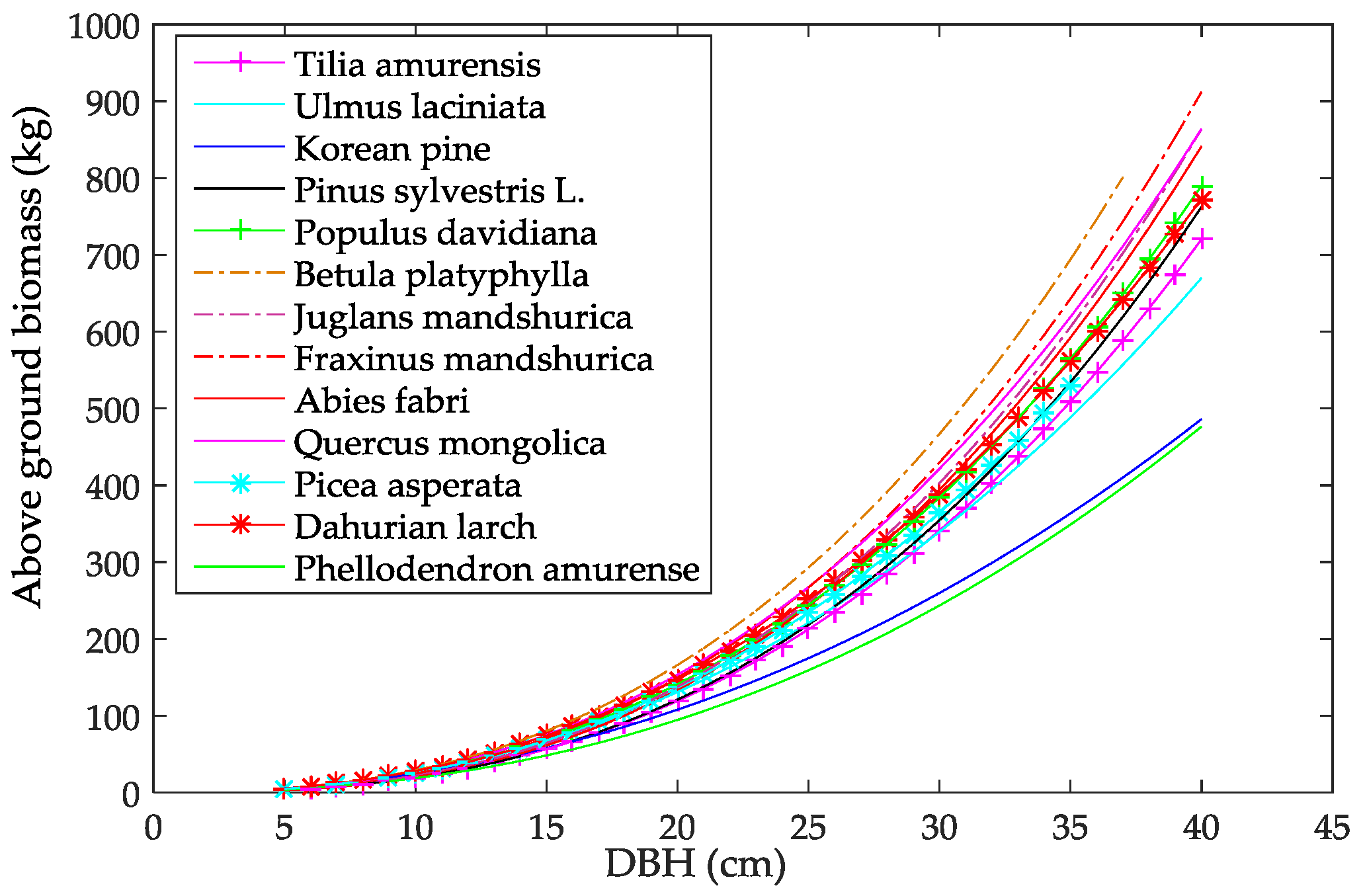
In the region studied in the current research, the single-tree biomass for each tree species was estimated using species-specific allometric equations [22,23,24,25,26,27] (Figure 3) obtained from the literature. The average aboveground biomass of each plot was then obtained by aggregating all single-tree biomass values in this plot and dividing by the area of the sampling plot.
The study region contained 148 field AGB data points. After matching with ICESat/GLAS data, during which the observed time, location, and ICESat/GLAS data quality were considered (see Section 2.2), a total of 108 plot data points were available for modeling (86 from the Sun et al. team and 22 from the Seventh National Forest Inventory dataset). Due to the lack of valid ICESat/GLAS data, 40 data points from the seventh National Forest Inventory dataset were left. The remaining 40 plot data points were used for independent validation of the AGB model using Landsat5/TM as input data.
2.2. ICESat/GLAS Data
The National Aeronautics and Space Administration (NASA) GLAS instrument staged in the Ice, Cloud, and Elevation Satellite (ICESat) is the first space-born full-waveform LiDAR sensor. GLAS emits a pulse waveform in 1064-nm bands, illuminating an elliptical surface footprint approximately 65 m in diameter, and records the returned waveform from the footprint. GLA01 (release 33), recording the transmitted and received waveforms, and GLA14 (release 34), recording the parameters obtained from GLA01 along with the geolocation of the footprint, were used in this study. GLAS shots that were less than 65 m away from field plots collected from the Seventh National Forest Inventory dataset were also used, as well as GLAS data corresponding to field plots from Sun et al. These GLAS data points were downloaded from the National Snow and Ice Data Center (NSIDC) website [28].
To obtain high-quality waveform data, filters are required. With reference to the screening methods proposed by Chi [29], Wu [30] and Baghdadi [31], GLAS data with no cloud and a signal-to-noise ratio (SNR) greater than 60 were retained. Cloudless GLAS data were identified using the cloud detection flag (i_FRir_qaflag = 15) in the GLA14 product [29,31]. In addition, the SNR values (Equation (1)) can be calculated using the fields i_max-RecAmp and i_sDevNsOb1 in the GLA14 product [30]. Here, i_max-RecAmp represents the peak amplitude of the received echo, and i_sDevNsOb1 represents the standard deviation of the background noise.
After filtering, a total of 108 waveform data points were available. Before calculating the waveform metrics associated with AGB, it was necessary to identify the three crucial locations of the waveform: the signal start location, the signal end location and the ground peak location, which relied on the processing described below.
1. Filtering the data
The waveform is commonly filtered by a Gaussian filter, which removes high-frequency noise and smooths the data [3,18]. In recent years, some researchers have used wavelet transforms to filter GLAS data [32]. This study compared the denoising effect of the two filters and selected the more effective filtering method. The wavelet transform steps followed in this paper were as follows: first, the signal was decomposed into three layers by a Gaussian wavelet; second, the high-frequency coefficients were denoised using a threshold; and finally, the coefficients underwent an inverse transformation [33]. As for the Gaussian filter, one was created with a width similar to the transmitted pulse and used to filter the original waveform [34].
Three indicators were selected to evaluate the filtering effects: root mean square error (RMSE) [35,36], signal-to-noise ratio (SNR) [35,36], and smoothness (r) [35]. The equations of these indicators can be expressed as follows:
where s is the original signal, f is the filtered signal, and N is the length of the signal.
2. Locating the signal start and end points
Noise was estimated from the signal intensity histogram before the signal start point and after the signal end point. When three consecutive bins were higher than the threshold (the sum of the noise mean and three standard deviations), the signal start and end were located [34].
3. Gaussian Decomposition
A Gaussian decomposition was applied to the filtered waveform using Levenberg-Marquardt nonlinear least-squares fitting [29,34,37]. To compare this method with the GLA14 product, the Pearson’s correlation coefficient (r) was calculated between the original waveform and the fitted waveforms obtained by the method described above and by the GLA14 product separately.
4. Identifying the ground peak
By reverse search from the signal endpoint, when the distance between the location of the Gaussian peak and the end of the signal was greater than half the emission pulse width, the location of the Gaussian peak was taken as the ground peak [34].
After processing the GLAS data using this method, waveform metrics sensitive to AGB were extracted according to methods in the available literature. These metrics were divided into two types, height metrics and intensity metrics, and their description and references can be found in Table 2. In addition to these metrics, the results of Gaussian decomposition, including location, amplitude, and width, were also used.
After testing the sensitivity to AGB of a number of variables from these GLAS parameters, eight variables (Treeht2, H25, LEE, TEE, HOME, QMCH, AVAW, and gasamp1 (the intensity of the first waveform from Gaussian decomposition)) were retained as predictor variables for GLAS data.
2.3. Landsat5/TM Data
The multispectral data used in this study were TM images with a resolution of 30 m, which matches the area of the field plots. One hundred eight (108) plots were distributed within the range of nine TM scenes. Cloud-free, good-quality images for each scene were downloaded from the United States Geological Survey (USGS) Earth Explorer as close as possible to the peak growing season. The collection duration (day of year (DOY)) of these images was limited to values from 180 to 210. To reduce the influence of spatial mismatch between the plots and the TM images, the mean reflectance was extracted from a 3 × 3 TM pixel window. The validity of the acquired TM images must also be checked by plotting the time-series curves of the spectral reflectances and vegetation indices before extracting variables, and data points that are obviously offset from the curve must be deleted.
The spectral variables extracted in this paper were divided into three categories:
- Surface reflectance: bands 1, 2, 3, 4, 5 and 7;
- Spectral indices: normalized difference vegetation index (NDVI) [42], Enhanced Vegetation index (EVI) [43] perpendicular vegetation index (PVI) [44], soil-adjusted vegetation index (SAVI) [45], normalized difference infrared vegetation index (NDIIB6) [46], normalized difference infrared vegetation index (NDIIB7) [46], [47], [47], and [47];
The formulae used can be found in Table 3.
For TM data, surface reflectance (band1 and band4), NDVI, , and TCW were retained as predictor variables, after selecting variables sensitive to AGB from the above TM parameters.
3. Methods
The methodology used to estimate forest AGB in this paper is shown in Figure 4.
First, field AGB was calculated based on models of the relationship between the measured data (tree species and DBH) and aboveground tree biomass [22,23,24,25,26,27] (Figure 3), as described in Section 2.1. The remote-sensing data parameters (GLAS metrics and TM variables) corresponding to field plots were then extracted using the methods described in Section 2.2 and Section 2.3.
In order to simplify the model and eliminate variables that are not sensitive to AGB and that are collinear with each other. We selected predictor variables for AGB modeling from the GLAS metrics and TM variables using stepwise regression analysis (see Section 3.1).
The dataset included 148 samples; each sample consists of these selected predictor variables and corresponding AGB field data. These samples were divided into two parts, one (108 samples) for modeling, and the other (40 samples) for validation. (1) For 108 samples, the modeling process was as follows: Bootstrapping was used to expand the modeling sample size, creating 300 bootstrap samples from the observations of size 108 (see Section 3.2). AGB models were developed for each bootstrap sample using three methods (stepwise regression (SR), support vector regression (SVR), and random forest (RF)) and three data sources (TM predictor variables, GLAS predictor variables, and TM predictor variables + GLAS predictor variables) (see Section 3.3). After comparing the results from modeling accuracy and cross validation, the optimal AGB model was determined. (2) For the remaining 40 samples, they were used for independent validation of the estimated AGB using the optimal model (see Section 3.4).
Finally, the forest AGB over the Daxing’anling Mountains was mapped using the optimal AGB model.
3.1. Variable Selection
In this study, many potential variables were extracted based on previous studies. Specifically, 42 GLAS variables (the parameters in Table 1 and the results of Gaussian decomposition) and 20 TM variables were available. Therefore, the first step was to determine the predictors to simplify the model and eliminate variables that are not related to AGB and that are collinear with each other. Stepwise regression analysis was used to pare down the potential variables. To test for collinearity between the selected variables, a variance inflation factor (VIF) threshold of 10 was used, with reference to the methods used by Powell [50]. VIF is an indicator of multicollinearity and is calculated as follows:
where is the VIF of the i-th variable and is the coefficient of determination of the regression equation between the i-th variable and the remaining variables. To calculate , first we run an ordinary least square regression that has Xi (i-th explanatory variable) as a function of all the other explanatory variables. The regression equation would be as follows:
where k is the total number of independent variables, c is a constant and e is the error term. Then the coefficient of determination of the regression Equation (6), , is calculated. In this case, we can calculate k different VIFs (one for each Xi). Generally, the value of VIF exceeding 10 is regarded as indicating multicollinearity. Particularly, in the process of paring down the variables, the variable with the largest VIF (greater than the selected threshold of 10) was the first one to be removed.
For ICESat/GLAS data, Treeht2, H25, LEE, TEE, HOME, QMCH, AVAW and gasamp1 (the intensity of the first waveform from Gaussian decomposition) were selected as predictor variables. The description of these variables is given in Table 2. For Landsat5/TM data, surface reflectances (band1 and band4), NDVI, were selected, as well as TCW.
3.2. Bootstrapping
In this study, the number of field data points available for modeling was only 108. To approximate the coefficient distributions and improve modeling accuracy, bootstrapping, which is a resampling technique, was applied to the regression in this paper [51,52].
Bootstrapping, which is a form of a sampling with replacement, initially proposed by Efron in 1797, has been widely used in many fields [52]. Unlike other sampling methods, there is no need to make assumptions about the form of the population [53]. It is a statistical inference method based on a sampling technique that can improve model estimation accuracy by increasing the number of samples [53].
The general bootstrapping process works as follows: a sample of size X is drawn from the original sample with replacement, where X is the size of the original sample. In this paper, the bootstrapping was combined with stratified sampling, so that bootstrap samples have similar overall properties to those 108 AGB data [52,53,54]. The steps were as follows:
- (1)
- The original data (AGB field data and corresponding predictor variables) of size 108 was sorted by ascending AGB values.
- (2)
- After that, we divided the dataset into four equal-sized subgroups (size = 27).
- (3)
- For each subgroup, random sampling with replacement was performed and repeated 27 times. Therefore, there were 27 data for each subgroup and a total of 108 data were obtained, which was our first bootstrap sample.
- (4)
- The process (3) was repeated 300 times to obtain 300 bootstrap samples.
In this paper, 300 bootstrap samples were created from the set of 108 observations and modeled separately.
3.3. Modeling Approach
In this paper, three prediction methods were considered: stepwise regression (SR), support vector regression (SVR), and random forest (RF). As shown in Figure 4, specifically, after the remote-sensing predictor variables were retained (see Section 3.1), 300 bootstrap samples were created as described in Section 3.2. Each bootstrap sample included predictor variables (8 variables for GLAS data and 5 variables for TM data) and corresponding AGB field data. For each bootstrap sample, three above modeling approaches (SR, SVR, and RF) and three input datasets (TM predictor variables, GLAS predictor variables, and TM predictor variables + GLAS predictor variables) were used to build AGB models respectively. As a result, nine AGB models were established for each bootstrap sample, namely, three SR AGB models (with TM predictor variables, with GLAS predictor variables, and with TM predictor variables + GLAS predictor variables), three SVR AGB models (with TM predictor variables, with GLAS predictor variables, and with TM predictor variables + GLAS predictor variables), and three RF AGB models (with TM predictor variables, with GLAS predictor variables, and with TM predictor variables + GLAS predictor variables).
SR is a parametric algorithm that is commonly used to estimate AGB [54]. The strength of this approach is that it can select suitable variables for the regression model when many explanatory variables are available. The idea of this algorithm is to introduce all the explanatory variables into the regression equation one by one according to their contributions to the dependent variable and to eliminate the variables whose effects are not significant after the introduction of new variables. In this paper, the underlying regression model used to evaluate the variables in the SR approach is multiple linear. Here, a significance level for deciding when to enter a predictor into the stepwise model is set to 0.15, like many software. Also, a significance level for deciding when to remove a predictor from the stepwise model is set to 0.15.
SVR and RF are two representative non-parametric algorithms that some studies have used to estimate AGB [14,50,54,55,56]. Unlike parametric algorithms, the strength of non-parametric algorithms is that they do not make assumptions about the form of the model and the distribution of input data, which makes it possible to effectively describe the complex nonlinear relationship between forest AGB and remote-sensing data [55]. SVR transforms a nonlinear regression into a linear regression by mapping the input data into a high-dimensional feature space using a kernel function. The essence of the solution is to find the optimal hyperplane based on the rule of structural risk minimization [56]. In this paper, the radial basis function kernel (RBF), which is the most widely used kernel function, was used because it requires fewer parameters and can reduce the difficulty of numerical calculation [57,58].
RF is an extension of the classification and regression tree (CART) approach. To improve prediction accuracy, random samples and attributes are selected to build multiple independent decision trees [59]. This algorithm is less sensitive to data noise and outliers than others [59]. A flowchart of the RF algorithm is shown in Figure 5. The original data are randomly resampled to yield N samples of size M by bagging repeatedly [59]. In this paper, the value of M (equal to the size of original data) is 108. In addition, the value of N (the number of trees) is 600, determined from the relationship between N and the error, which is also commonly used to determine the number of trees. Then a regression tree is constructed for each dataset. For each regression tree, each node is split using a random subset of size mtry (the number of predictors sampled for splitting) from the features, a procedure called “feature bagging”. The result is estimated by averaging the predictions of the N regression trees. In this paper, the value of mtry was selected based on the RMSE of the data not included in each sample, an approach that is called out-of-bag (OOB) data.
In the modeling process, the above algorithms were implemented in R, an open-source software environment [60,61]. For each bootstrap sample, three modeling approaches (SR, SVR, and RF) and three input datasets (TM, GLAS, and TM + GLAS) were used. During which, cross validation was performed with four-fold and five repetitions for each prediction model, which means that 75% of the input data was training data and the rest was test data. After comparison and evaluation, the optimal AGB model was indicated by R-squared (R2) and root mean square error (RMSE) from both modeling accuracy and cross validation.
3.4. Independent Validation
Due to the lack of corresponding GLAS data, there were 40 field plots that were not used for modeling. To perform further validation of the selected model (the RF AGB model with TM data), these plots were used for independent validation. In addition to R2 and RMSE, another model evaluation index, the total relative error (TRE) (Equation (7)), which was proposed by Zeng [62], was also used to evaluate the forest AGB model:
where is the i-th measured value, and is the i-th predicted value from the model. TRE is an important indicator reflecting the effect of model fitting and should be controlled within a certain range (such as ±3% or ±5%).
4. Results
4.1. ICESat/GLAS Data Processing Results
In order to calculate the waveform metrics associated with AGB, it was necessary to pre-process the GLAS raw data. In the process of Filtering and Gaussian Decomposition, the results of different methods were compared and analyzed.
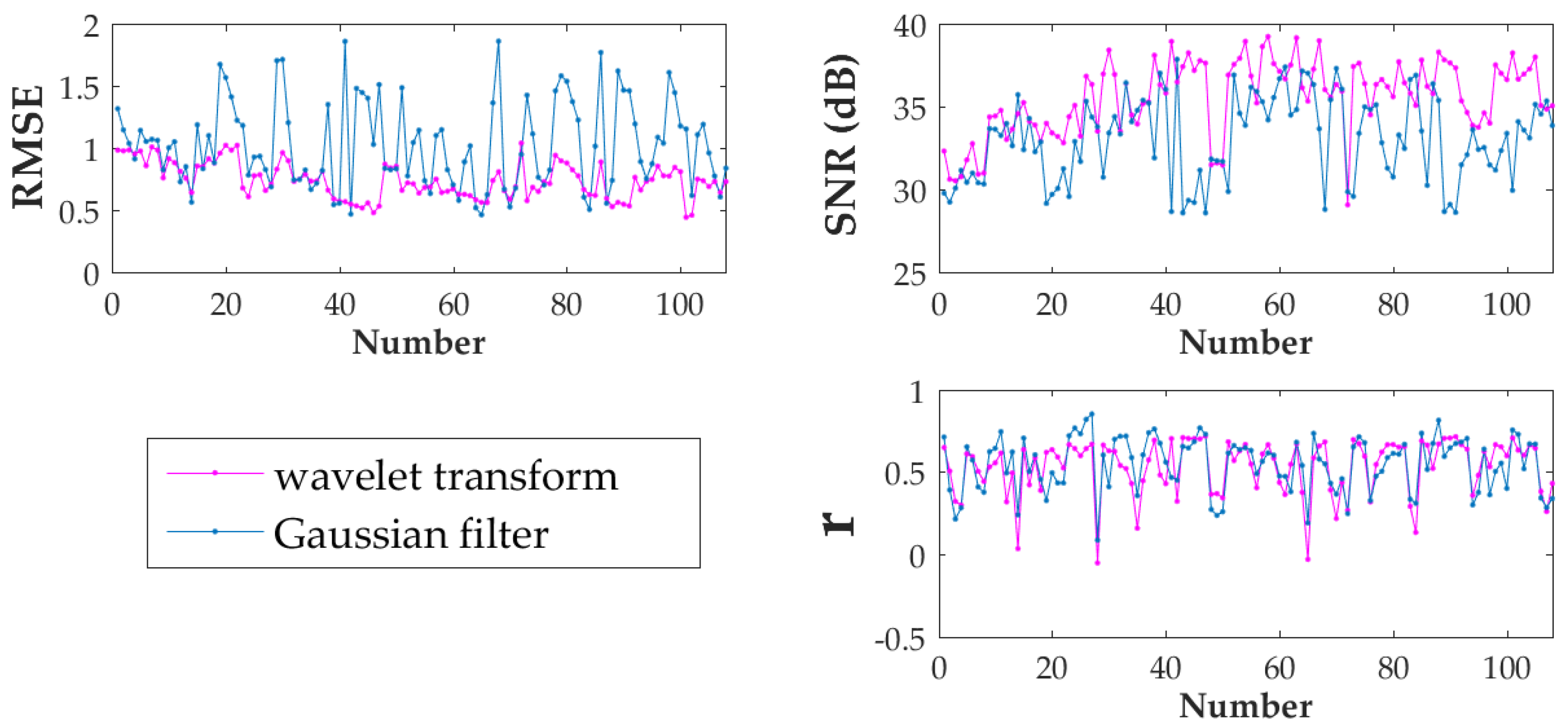
Comparison of the filtering effects of wavelet transform and Gaussian filter (Figure 6 and Table 4) showed that the RMSE and SNR of the wavelet transform were better than those of the Gaussian filter, but that the smoothness was not significantly different. As a result, the wavelet transform was chosen to filter the waveform of the GLAS footprint.
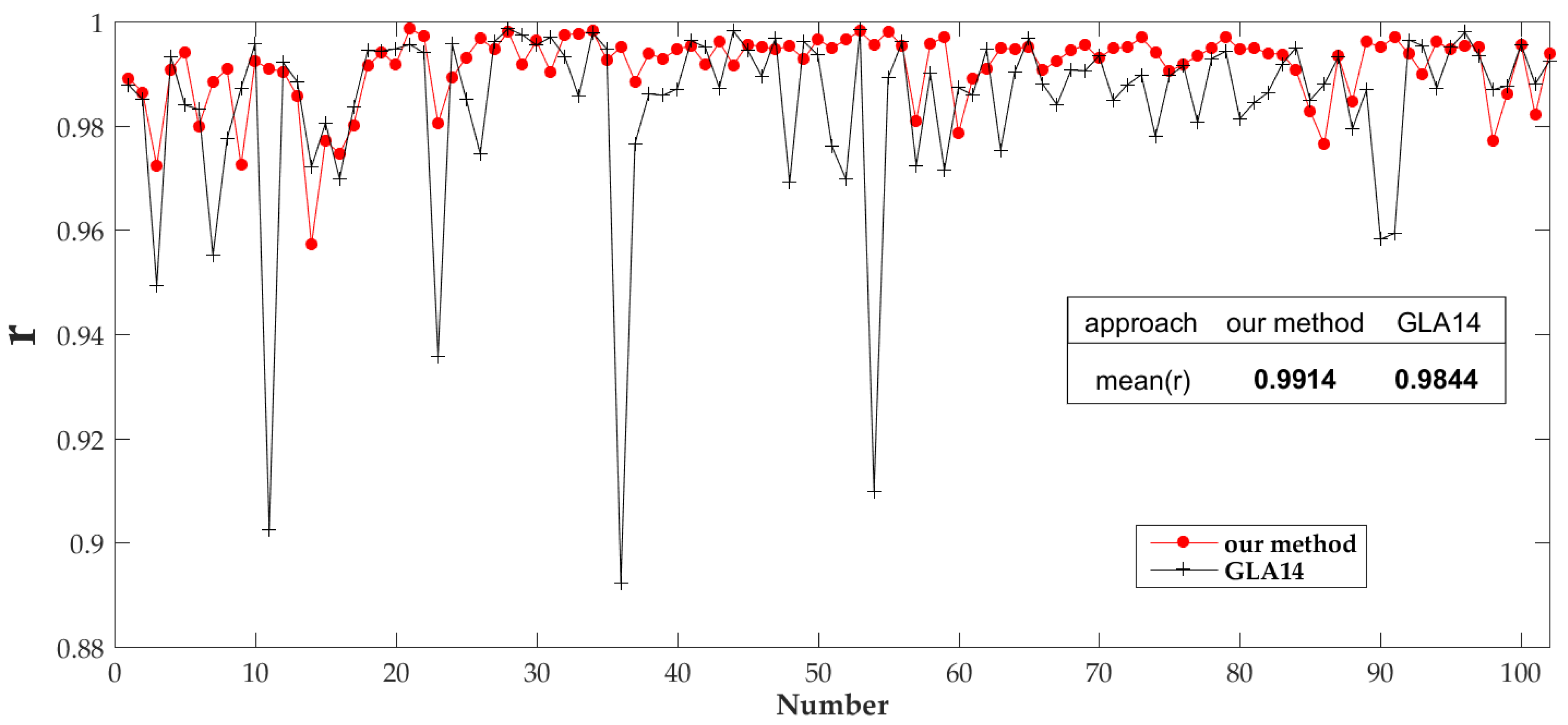
As mentioned in Section 2.2, the Pearson’s correlation coefficient (r) was calculated between the original waveform and the fitted waveforms obtained by the proposed method and by the GLA14 product separately. A comparison of these two correlations is shown in Figure 7. Clearly, the overall correlation obtained using the proposed method is superior to that obtained using the GLA14 product.
After processing the GLAS data using the above method, three crucial locations of the waveform (the signal start location, the signal end location and the ground peak location) were successfully identified. In addition, then the waveform metrics in Table 2 were extracted.
4.2. AGB Model Results
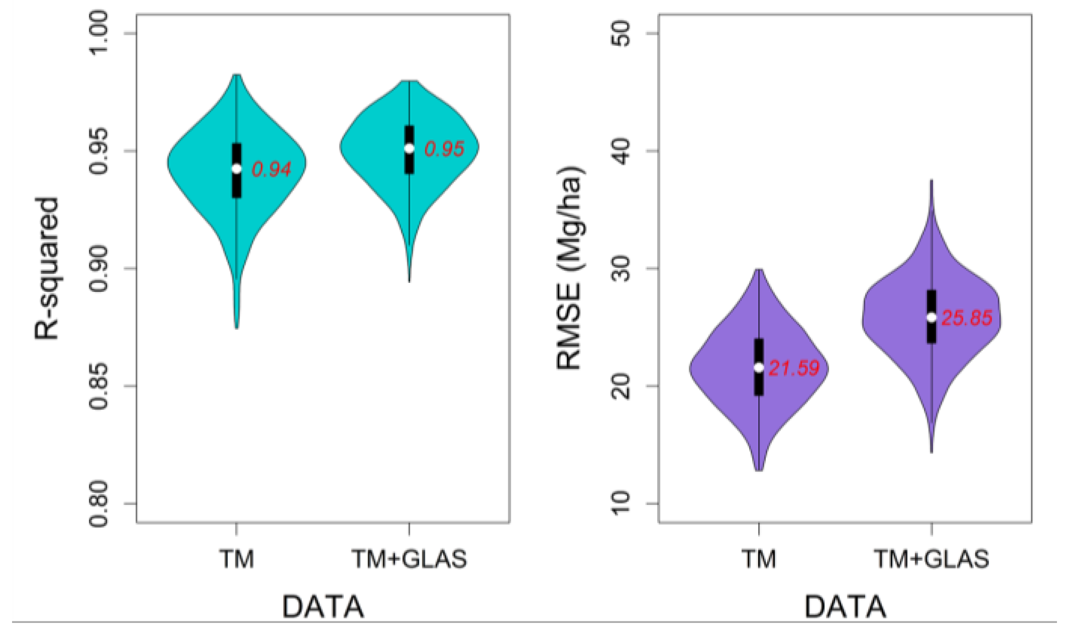
The performances of all AGB models, evaluated in terms of R2 and RMSE, is shown in Figure 8 and Figure 9. Figure 8 summarizes the modeling accuracy results from regression using different approaches and input data combined with bootstrapping, and Figure 9 shows the results from repeated cross validation. RF outperformed the other two approaches in all three cases: with TM data alone, with GLAS data alone, and with GLAS data and TM data together. RF AGB models generally led to higher R2 and smaller RMSE, both in modeling accuracy (R2max = 0.96, RMSEmin = 17.73 Mg/ha) and cross validation (R2max = 0.76, RMSEmin = 39.60 Mg/ha). The performance of the SR AGB models was the worst in terms of R2 and RMSE for both modeling accuracy and cross validation. The presence of GLAS data significantly improved AGB predictions for SVR and SR AGB models by decreasing RMSE and increasing R2. As for the RF AGB models, inclusion of GLAS data no longer led to significant improvement. There was little difference in terms of R2 and RMSE between the RF AGB model with TM alone and that with GLAS or TM + GLAS. Considering that the GLAS footprints are spatially discontinuous, this model needs to be extrapolated at regional scale by adding more data, which will introduce new errors at the same time. Therefore, in this paper, the Landsat5/TM dataset was used as input data with RF as the prediction method to estimate forest AGB at regional scale.
The performance of the RF AGB model with TM data was further investigated. Scatter plots of field AGB against predicted biomass from RF models with 300 bootstraps is shown in Figure 10. The distribution of scatter points is concentrated near the 1:1 line, but this model underestimated forest AGB at high AGB levels (200–400 Mg/ha) and overestimated it at low AGB levels (0–200 Mg/ha). The modeling accuracy results of RF AGB models created with different sample sizes (Figure 11) show that increasing the sample size led to an increase in R2, a decrease in RMSE, and a reduction in the range of variation, implying that the established model is more stable.
Sixty-nine samples, which were randomly selected from the 108 datasets, were used for RF AGB modeling with TM and TM + GLAS respectively. The modeling accuracy results (Figure 12) further confirmed the previous finding that the presence of GLAS data did not lead to a significant increase in R2. In this case, inclusion of GLAS data resulted in an increase in RMSE.
To perform further validation of the selected model (the RF AGB model with TM data), the remaining 40 plots were used for independent validation (Figure 13). The predicted forest AGB values were the medians of the 300 bootstrap estimates. The results show an R2 of 0.54, an RMSE of 20.5 Mg/ha and a TRE of 4.97%, which was within the acceptable range.
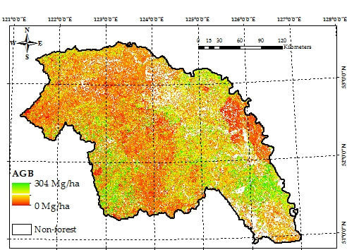
4.3. Wall-to-Wall AGB Prediction over the Daxing’anling Mountains in Heilongjiang Province
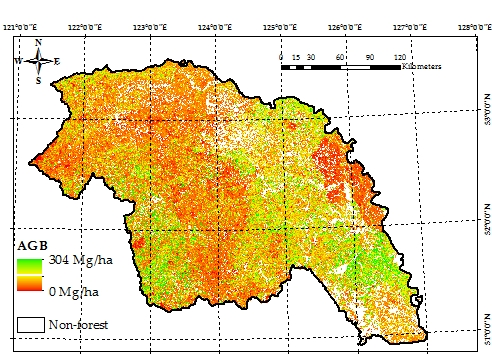
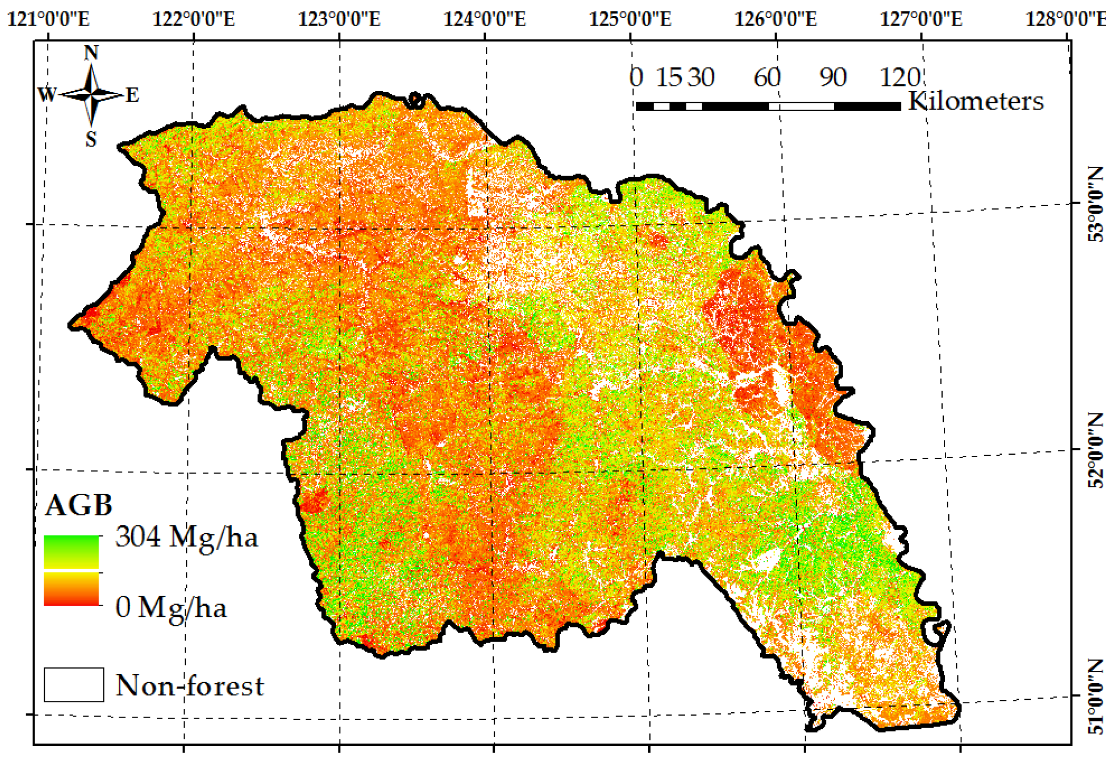
The spatial distribution of forest AGB density in 2005 over the Daxing’anling Mountains is shown in Figure 14, using the optimal AGB model established in Section 4.1. The predicted forest AGB density values were the medians of the 300 bootstrap estimates. The forest AGB density over the Daxing’anling Mountains was distributed mainly in the 60–90 Mg/ha range, and the highest value was 304 Mg/ha. The average forest AGB density over the Daxing’anling Mountains was 83.13 Mg/ha. This value is close to the average AGB density, 83.50–102.49 Mg/ha, estimated by Zhang et al. [3] in northeastern China, who also found that the forest AGB of the Daxing’anling Mountains was less than those of the Changbai and Xiaoxing’anling Mountains. The result obtained here is slightly larger than the 80.18 Mg/ha provided by Huang and Xia [64] using the Dong model in northeastern China.
5. Discussion
In this paper, the results of models using different datasets and three approaches were compared. The random forest AGB model using Landsat5/TM as input data has the acceptable modeling accuracy (R2 = 0.95 RMSE = 17.73 Mg/ha) and it was also shown to estimate AGB reliably by cross validation (R2 = 0.71 RMSE = 39.60 Mg/ha). We also compared our results with other similar research works. Powell [50] modeled aboveground tree biomass using field data and Landsat satellite imagery in Minnesota and Arizona by comparing different statistical techniques. The RMSE of the modeling accuracy results ranged from 32.19 to 44.43 Mg/ha. Zhang et al. [3] developed forest AGB models in northeastern China based on GLAS data, achieving an R2 of modeling accuracy results for field-measured points of 0.86 and an RMSE of 26.76 Mg/ha. Compared with other published studies, the forest AGB model in this paper achieved better performance in terms of modeling accuracy (R2 and RMSE).
5.1. Spatio-Temporal Matching between GLAS Data and Measured Data
When matching the measured field data and the GLAS waveforms, it was assumed that no significant change in forest AGB in the field plot had occurred within the previous three years. In terms of geographical location, especially for matching forest inventory data with GLAS data, the authors believe that a central location difference in the 65-m range is acceptable. The above assumptions are due to the difficulty of matching the two datasets, which is caused by the short observation time of GLAS, the small number of repeated observations, and the spatial discontinuities of GLAS. To make these hypotheses reasonable, the spectral difference of the plots between the GLAS observation time and the measurement time were examined, and the spectral variance from a 3 × 3 TM pixel window corresponding to the GLAS data was also examined. Data points with an abnormal deviation were deleted.
The modeling accuracy and cross validation results showed that selection of representative GLAS data for the field plots is an important step towards effective modeling and improved modeling accuracy.
5.2. GLAS Data and Terrain Effects
LiDAR waveforms are susceptible to ground slopes. When the ground slope is greater than 20 degrees, information from the ground and from the canopy are intermixed, making the extracted metrics no longer accurate [65,66]. Before modeling, slope values were calculated for all field plots, and all were found to be less than 20 degrees, with most less than 15 degrees.
In addition, an effort was made to add auxiliary data in the form of a digital elevation model (DEM) to the model, but the results were not improved. Therefore, terrain effects were not taken into account in this paper, but when the GLAS model is applied to complex terrain, terrain effects must be eliminated.
5.3. Influence of Regional Coverage Types on Estimation
The field measurements used in this paper consisted of two parts, one from measurements of the GLAS footprints, where three sampling plots were established within each footprint, and the other from National Forest Inventory data, where each tree with DBH greater than 5 cm in the range of 0.06 ha was measured. The difference in sampling methods between these two datasets may have introduced errors to the results. Only the tree biomass was involved in field measurements, ignoring shrubs and herbaceous plants. Therefore, the resulting estimates of forest AGB were lower than the actual values.
5.4. Effects of TM Data on Regional Biomass Mapping
In this modeling exercise, the acquisition time of the TM images was close to the peak of the growing season, and the time differences among scenes were less than 30 days. The results were highly affected by TM data quality when the AGB model was applied at regional scale. In this research, the TM data for the study area close to the growing season in 2005 were of good quality, and most areas were clear. However, the model will be limited when good-quality TM data are unavailable for the entire growing season, which is highly probable in some areas. In this case, TM image reconstruction methods can be used to compensate for the lack of data.
5.5. Effects of range of AGB values on validation
The RMSE from independent validation using the 40-sample dataset is significantly lower than the RMSE from cross validation, which may due to the range of AGB values measured on the field plots. In particular, the AGB values of 40-sample dataset for independent validation were within the smaller AGB (AGB < 160 Mg/ha) (see Figure 13), while the range of AGB used in the modeling was 0–400 Mg/ ha, with the main distribution values ranging from 0–160 Mg/ha. Therefore, the RMSE from independent validation is smaller. In addition, the larger RMSE result from cross validation is mainly affected by the large-values of AGB data.
6. Conclusions
To map the distribution of forest AGB density at regional scale, two types of remote-sensing data matching were selected for a group of field plots: optical remote-sensing data (Landsat5/TM) with a resolution of 30 m, and LiDAR data (ICESat/GLAS) with a footprint approximately 65 m in diameter. AGB models were built using these field measurements and remote-sensing datasets. The results showed that including GLAS data improved AGB predictions for the SR and SVR AGB models. However, for the RF AGB models, there was little difference between the results from the three input datasets. Therefore the combination of data type and prediction method is important, and LiDAR data (e.g., GLAS data) may not be a necessary option for estimating forest AGB. After comparing and analyzing the effects of the various AGB models using the three modeling approaches and three remote-sensing datasets combined with bootstrapping, it was found that the RF AGB model with TM data was optimal for mapping. Finally, forest AGB density with spatial resolution of 30 m over the Daxing’anling Mountains was mapped. Compared with some other researches, the estimated forest AGB at the regional scale is acceptable.
Acknowledgments
This research was supported by the National Basic Research Program of China under grant No. 2013CB733403. The authors would also like to express gratitude to Sun Guoqing, who provided field measurements for this research, and Zhang Yuzhen, who provide much help and instruction in data processing.
Author Contributions
Kaili Liu designed the framework of this research work and wrote the manuscript; Jindi Wang proposed the main idea, provided important guidance on the work, and checked the writing; Weisheng Zeng provided the field data and guidance; and Jinling Song gave guidance on this work.
Conflicts of Interest
The authors declare no conflict of interest.
References
- Olson, J.S.; Watts, J.A.; Allison, L.J. Carbon in Live Vegetation of Major World Ecosystems; Oak Ridge National Laboratory: Oak Ridge, TN, USA, 1983.
- Brown, S.; Sathaye, J.; Cannell, M.; Cannell, M.; Kauppi, P.E. Mitigation of carbon emissions to the atmosphere by forest management. Commonw. For. Rev. 1996, 75, 80–91. [Google Scholar]
- Zhang, Y.; Liang, S.; Sun, G. Forest biomass mapping of northeastern China using GLAS and MODIS data. IEEE J. Sel. Top. Appl. Earth Obs. Remote Sens. 2014, 7, 140–152. [Google Scholar] [CrossRef]
- Lu, D. The potential and challenge of remote sensing–based biomass estimation. Int. J. Remote Sens. 2006, 27, 1297–1328. [Google Scholar] [CrossRef]
- McRoberts, R.E.; Næsset, E.; Gobakken, T. Inference for lidar-assisted estimation of forest growing stock volume. Remote Sens. Environ. 2013, 128, 268–275. [Google Scholar] [CrossRef]
- Ahamed, T.; Tian, L.; Zhang, Y.; Ting, K.C. A review of remote sensing methods for biomass feedstock production. Biomass Bioenergy 2011, 35, 2455–2469. [Google Scholar] [CrossRef]
- Lu, D.; Batistella, M.; Moran, E. Satellite estimation of aboveground biomass and impacts of forest stand structure. Photogramm. Eng. Remote Sens. 2005, 71, 967–974. [Google Scholar] [CrossRef]
- Dobson, M.C.; Ulaby, F.T.; LeToan, T.; Beaudoin, A. Dependence of radar backscatter on coniferous forest biomass. IEEE Trans. Geosci. Remote Sens. 1992, 30, 412–415. [Google Scholar] [CrossRef]
- Drake, J.B.; Dubayah, R.O.; Clark, D.B.; Knox, R.G.; Blair, J.B.; Hofton, M.A.; Chazdone, R.L.; Weishampelf, J.F.; Prince, S. Estimation of tropical forest structural characteristics using large-footprint lidar. Remote Sens. Environ. 2002, 79, 305–319. [Google Scholar] [CrossRef]
- Yu, Y.; Yang, X.; Fan, W. Estimates of forest structure parameters from GLAS data and multi-angle imaging spectrometer data. Int. J. Appl. Earth Obs. Geoinform. 2015, 38, 65–71. [Google Scholar] [CrossRef]
- Mougin, E.; Proisy, C.; Marty, G.; Fromard, F.; Puig, H.; Betoulle, J.L.; Rudant, J.P. Multifrequency and multipolarization radar backscattering from mangrove forests. IEEE Trans. Geosci. Remote Sens. 1999, 37, 94–102. [Google Scholar] [CrossRef]
- Sandberg, J.; Tsoukas, H. Grasping the logic of practice: Theorizing through practical rationality. Acad. Manag. Rev. 2011, 36, 338–360. [Google Scholar] [CrossRef]
- Hajj, M.E.; Baghdadi, N.; Fayad, I.; Vieilledent, G.; Bailly, J.S.; Minh, D.H.T. Interest of integrating spaceborne LiDAR data to improve the estimation of biomass in high biomass forested areas. Remote Sens. 2017, 9, 213. [Google Scholar] [CrossRef]
- Fayad, I.; Baghdadi, N.; Guitet, S.; Bailly, J.S.; Hérault, B.; Gond, V.; Hajj, M.E.; Minh, D.H.T. Aboveground biomass mapping in French Guiana by combining remote sensing, forest inventories and environmental data. Int. J. Appl. Earth Obs. Geoinform. 2016, 52, 502–514. [Google Scholar] [CrossRef]
- Lu, D.; Chen, Q.; Wang, G.; Liu, L.; Li, G.; Moran, E. A survey of remote sensing-based aboveground biomass estimation methods in forest ecosystems. Int. J. Digit. Earth 2016, 9, 63–105. [Google Scholar] [CrossRef]
- Dixon, R.K.; Brown, S.; Houghton, R.E.A.; Solomon, A.M.; Trexler, M.C.; Wisniewski, J. Carbon pools and flux of global forest ecosystems. Science 1994, 263, 185–190. [Google Scholar] [CrossRef] [PubMed]
- Saatchi, S.; Malhi, Y.; Zutta, B.; Buermann, W.; Anderson, L.O.; Araujo, A.M.; Phillips, O.L.; Peacock, J.; Steege, H.T.; Gonzalez, G.L.; et al. Mapping landscape scale variations of forest structure, biomass, and productivity in Amazonia. Biogeosci. Discuss. 2009, 6, 5461–5505. [Google Scholar] [CrossRef]
- Pang, Y.; Lefsky, M.; Sun, G.; Miller, M.E.; Li, Z. Temperate forest height estimation performance using ICESat GLAS data from different observation periods. Int. Arch. Photogramm. Remote Sens. Spat. Inf. Sci. 2008, 37, 777–782. [Google Scholar]
- Sun, G.; Ranson, K.; Masek, J.; Guo, Z.; Pang, Y.; Fu, A.; Wang, D. Estimation of tree height and forest biomass from GLAS data. J. For. Plan. 2008, 13, 157–164. [Google Scholar]
- Chen, X.; Zeng, W.; Xiong, Z.; Zhang, M. New development of China National Forest Inventory (NFI)—On revision of NFI technical regulations. For. Resour. Manag. 2004, 5, 40–45. [Google Scholar]
- Chen, J.; Chen, J.; Liao, A.; Cao, X.; Chen, L.; Chen, X.; He, C.; Han, G.; Peng, S.; Lu, M.; et al. Global land cover mapping at 30 m resolution: A POK-based operational approach. ISPRS J. Photogramm. Remote Sens. 2014, 103, 7–27. [Google Scholar] [CrossRef]
- Zeng, W. Methodoly on Moeling of Single-Tree Biomass Equations for National Biomass Estimation in China. Ph.D. Thesis, Chinese Academy of Forestry, Beijing, China, 2011. (In Chinese). [Google Scholar]
- Zeng, W.S.; Zhang, H.R.; Tang, S.Z. Using the dummy variable model approach to construct compatible single-tree biomass equations at different scales—A case study for Masson pine (Pinus massoniana) in southern China. Can. J. For. Res. 2011, 41, 1547–1554. [Google Scholar] [CrossRef]
- Dong, L.; Zhang, L.; Li, F. Developing additive systems of biomass equations for nine hardwood species in Northeast China. Trees 2015, 29, 1149–1163. [Google Scholar] [CrossRef]
- Wang, H. Dynamic Simulating System for Stand Growth of Forest in Northeast China. Ph.D. Thesis, Northeast Foreast University, Harbin, China, 2012. (In Chinese). [Google Scholar]
- Wang, C. Biomass allometric equations for 10 co-occurring tree species in Chinese temperate forests. For. Ecol. Manag. 2006, 222, 9–16. [Google Scholar] [CrossRef]
- Dong, L.; Zhang, L.; Li, F. A compatible system of biomass equations for three conifer species in northeast, China. For. Ecol. Manag. 2014, 329, 306–317. [Google Scholar] [CrossRef]
- National Snow & Ice Data Center. Available online: http://nsidc.org/ (accessed on 2 April 2017).
- Chi, H.; Sun, G.; Huang, J.; Guo, Z.; Ni, W.; Fu, A. National forest aboveground biomass mapping from ICESat/GLAS data and MODIS imagery in China. Remote Sens. 2015, 7, 5534–5564. [Google Scholar] [CrossRef]
- Wu, D.; Fan, W. Synergistic use of ICESat/GLAS and MISR data for estimating forest aboveground biomass. Bull. Bot. Res. 2015, 3, 397–405. (In Chinese) [Google Scholar]
- Baghdadi, N.; El Hajj, M.; Bailly, J.S.; Fabre, F. Viability statistics of GLAS/ICESat data acquired over tropical forests. IEEE J. Sel. Top. Appl. Earth Obs. Remote Sens. 2014, 7, 1658–1664. [Google Scholar] [CrossRef]
- Pourrahmati, M.R.; Baghdadi, N.N.; Darvishsefat, A.A.; Namiranian, M.; Fayad, I.; Bailly, J. S.; Gond, V. Capability of GLAS/ICESat data to estimate forest canopy height and volume in mountainous forests of Iran. IEEE J. Sel. Top. Appl. Earth Obs. Remote Sens. 2015, 8, 5246–5261. [Google Scholar] [CrossRef]
- Sihag, R. Wavelet thresholding for image de-noising. In Proceedings of the International Conference on VLSI, Communication & Instrumentation (ICVCI), Kottayam, Kerala, India, 7–9 April 2011; Volume 201, pp. 20–23. [Google Scholar]
- Sun, G.; Ranson, K.; Kimes, D.; Blair, J.B.; Kovacs, K. Forest vertical structure from GLAS: An evaluation using LVIS and SRTM data. Remote Sens. Environ. 2008, 112, 107–117. [Google Scholar] [CrossRef]
- Yang, H.; Zhang, D.; Huang, W.; Gao, Z.; Yang, X.; Li, C.; Wang, J. Application and evaluation of wavelet-based denoising method in hyperspectral imagery data. In Proceedings of the International Conference on Computer and Computing Technologies in Agriculture, Beijing, China, 29–31 October 2011; Springer: Berlin/Heidelberg, Germany, 2011; pp. 461–469. [Google Scholar]
- Yi, T.-H.; Li, H.-N.; Zhao, X.-Y. Noise smoothing for structural vibration test signals using an improved wavelet thresholding technique. Sensors 2012, 12, 11205–11220. [Google Scholar] [CrossRef] [PubMed]
- Ranson, K.J.; Kimes, D.; Sun, G.; Nelson, R.; Kharuk, V.; Montesano, P. Using MODIS and GLAS data to develop timber volume estimates in central Siberia. In Proceedings of the 2007 IEEE International Geoscience and Remote Sensing Symposium, Barcelona, Spain, 23–28 July 2007; pp. 2306–2309. [Google Scholar]
- Lefsky, M.A.; Keller, M.; Pang, Y.; De Camargo, P.B.; Hunter, M.O. Revised method for forest canopy height estimation from Geoscience Laser Altimeter System waveforms. J. Appl. Remote Sens. 2007, 1, 013537. [Google Scholar]
- Kimes, D.S.; Ranson, K.J.; Sun, G.; Blair, J.B. Predicting lidar measured forest vertical structure from multi-angle spectral data. Remote Sens. Environ. 2006, 100, 503–511. [Google Scholar] [CrossRef]
- Lefsky, M.A.; Harding, D.; Cohen, W.B.; Parker, G.; Shugart, H.H. Surface lidar remote sensing of basal area and biomass in deciduous forests of eastern Maryland, USA. Remote Sens. Environ. 1999, 67, 83–98. [Google Scholar] [CrossRef]
- Harding, D.J.; Carabajal, C.C. ICESat waveform measurements of within-footprint topographic relief and vegetation vertical structure. Geophys. Res. Lett. 2005, 32, 322. [Google Scholar] [CrossRef]
- Rouse, J.W.; Haas, R.H.; Schell, J.A.; Deering, D.W. Monitoring Vegetation Systems in the Great Plains with ERTS; NASA Special Publication; NASA: Washington, DC, USA, 1974; Volume 351, p. 309.
- Huete, A.; Didan, K.; Miura, T.; Rodriguez, E.P.; Gao, X.; Ferreira, L.G. Overview of the radiometric and biophysical performance of the MODIS vegetation indices. Remote Sens. Environ. 2002, 83, 195–213. [Google Scholar] [CrossRef]
- Richardson, A.J.; Wiegand, C.L. Distinguishing vegetation from soil background information. Photogramm. Eng. Remote Sens. 1978, 43, 1541–1552. [Google Scholar]
- Huete, A.R. A soil-adjusted vegetation index (SAVI). Remote Sens. Environ. 1988, 25, 295–309. [Google Scholar] [CrossRef]
- Hunt, E.R.; Rock, B.N. Detection of changes in leaf water content using near-and middle-infrared reflectances. Remote Sens. Environ. 1989, 30, 43–54. [Google Scholar]
- Cai, T.; Ju, C.; Yao, Y. Quantitative estimation of vegetation coverage in Mu Us sandy land based on RS and GIS. Chin. J. Appl. Ecol. 2005, 16, 2301–2305. (In Chinese) [Google Scholar]
- Crist, E.P. A TM Tasseled Cap equivalent transformation for reflectance factor data. Remote Sens. Environ. 1985, 17, 301–306. [Google Scholar] [CrossRef]
- Duane, M.V.; Cohen, W.B.; Campbell, J.L.; Hudiburg, T.; Turner, D.P.; Weyermann, D.L. Implications of alternative field-sampling designs on landsat-based mapping of stand age and carbon stocks in oregon forests. For. Sci. 2010, 21, 77–79. [Google Scholar]
- Powell, S.L.; Cohen, W.B.; Healey, S.P.; Kennedy, R.E.; Moisen, G.G.; Pierce, K.B.; Ohmann, J.L. Quantification of live aboveground forest biomass dynamics with Landsat time-series and field inventory data: A comparison of empirical modeling approaches. Remote Sens. Environ. 2010, 114, 1053–1068. [Google Scholar] [CrossRef]
- Juan, S.; Lantz, F. Application of bootstrap techniques in econometrics: The example of cost estimation in the automotive industry. Oil Gas Sci. Technol. 2001, 56, 373–388. [Google Scholar] [CrossRef]
- Wehrens, R.; Putter, H.; Buydens, L.M.C. The bootstrap: A tutorial. Chemom. Intell. Lab. Syst. 2000, 54, 35–52. [Google Scholar] [CrossRef]
- Freedman, D.A. Bootstrapping regression models. Ann. Stat. 1981, 9, 1218–1228. [Google Scholar] [CrossRef]
- Fassnacht, F.E.; Hartig, F.; Latifi, H.; Berger, C.; Hernández, J.; Corvalán, P.; Koch, B. Importance of sample size, data type and prediction method for remote sensing-based estimations of aboveground forest biomass. Remote Sens. Environ. 2014, 154, 102–114. [Google Scholar] [CrossRef]
- Avitabile, V.; Baccini, A.; Friedl, M.A.; Schmullius, C. Capabilities and limitations of Landsat and land cover data for aboveground woody biomass estimation of Uganda. Remote Sens. Environ. 2012, 117, 366–380. [Google Scholar] [CrossRef]
- Zhao, K.; Popescu, S.; Meng, X.; Pang, Y.; Agca, M. Characterizing forest canopy structure with lidar composite metrics and machine learning. Remote Sens. Environ. 2011, 115, 1978–1996. [Google Scholar] [CrossRef]
- Müller, K.-R.; Mika, S.; Rätsch, G.; Tsuda, K.; Schölkopf, B. An introduction to kernel-based learning algorithms. IEEE Trans. Neural Netw. 2001, 12, 181–201. [Google Scholar] [CrossRef] [PubMed]
- Crone, S.F.; Lessmann, S.; Pietsch, S. Parameter sensitivity of support vector regression and neural networks for forecasting. In Proceedings of the IEEE International Conference on Data Mining (DMIN), Hongkong, China, 18–22 December 2006; pp. 396–402. [Google Scholar]
- Breiman, L. Random forests. Mach. Learn. 2001, 45, 5–32. [Google Scholar] [CrossRef]
- Ihaka, R.; Gentleman, R. R: A language for data analysis and graphics. J. Comput. Grph. Stat. 1996, 5, 299–314. [Google Scholar] [CrossRef]
- Dalgaard, P. Introductory statistics with R. J. R. Stat. Soc. Ser. A Stat. Soc. 2009, 172, 274–275. [Google Scholar]
- Zeng, W.; Tang, S. Goodness evaluation and precision of tree biomass equations. Sci. Silvae Sin. 2011, 47, 106–113. [Google Scholar]
- Potter, K.; Hagen, H.; Kerren, A.; Dannenmann, P. Methods for presenting statistical information: The box plot. Vis. Larg. Unstruct. Data Sets S 2006, 4, 97–106. [Google Scholar]
- Huang, G.; Xia, C. MODIS-based estimation of forest biomass in northeast China. For. Resour. Manag. 2005, 4, 40–44. (In Chinese) [Google Scholar]
- Pang, Y.; Li, Z.; Lefsky, M.; Sun, G.; Yu, X. Model based terrain effect analyses on ICEsat GLAS waveforms. In Proceedings of the 2006 IEEE International Symposium on Geoscience and Remote Sensing, Vancouver, BC, Canada, 28–30 August 2006; pp. 3232–3235. [Google Scholar]
- Wang, X.; Huang, H.; Gong, P.; Liu, C.; Li, C.; Li, W. Forest canopy height extraction in rugged areas with ICESAT/GLAS data. IEEE Trans. Geosci. Remote Sens. 2014, 52, 4650–4657. [Google Scholar] [CrossRef]
Figure 1.
Locations of field plots and GLAS data. The red dots represent field measurements from Sun et al. [18,19]. The purple dots represent data from the Seventh National Forest Inventory. The black dots represent GLAS L3C footprints. The background information is a 30-m forest distribution (in green) map developed by Chen [21].
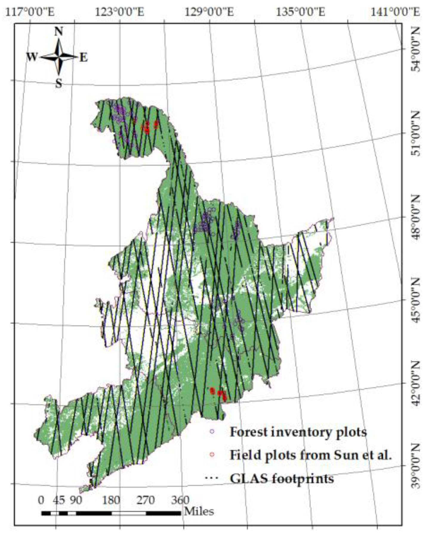
Figure 2.
Schematic diagram of field sampling. The solid blue circles represent sampling plots.
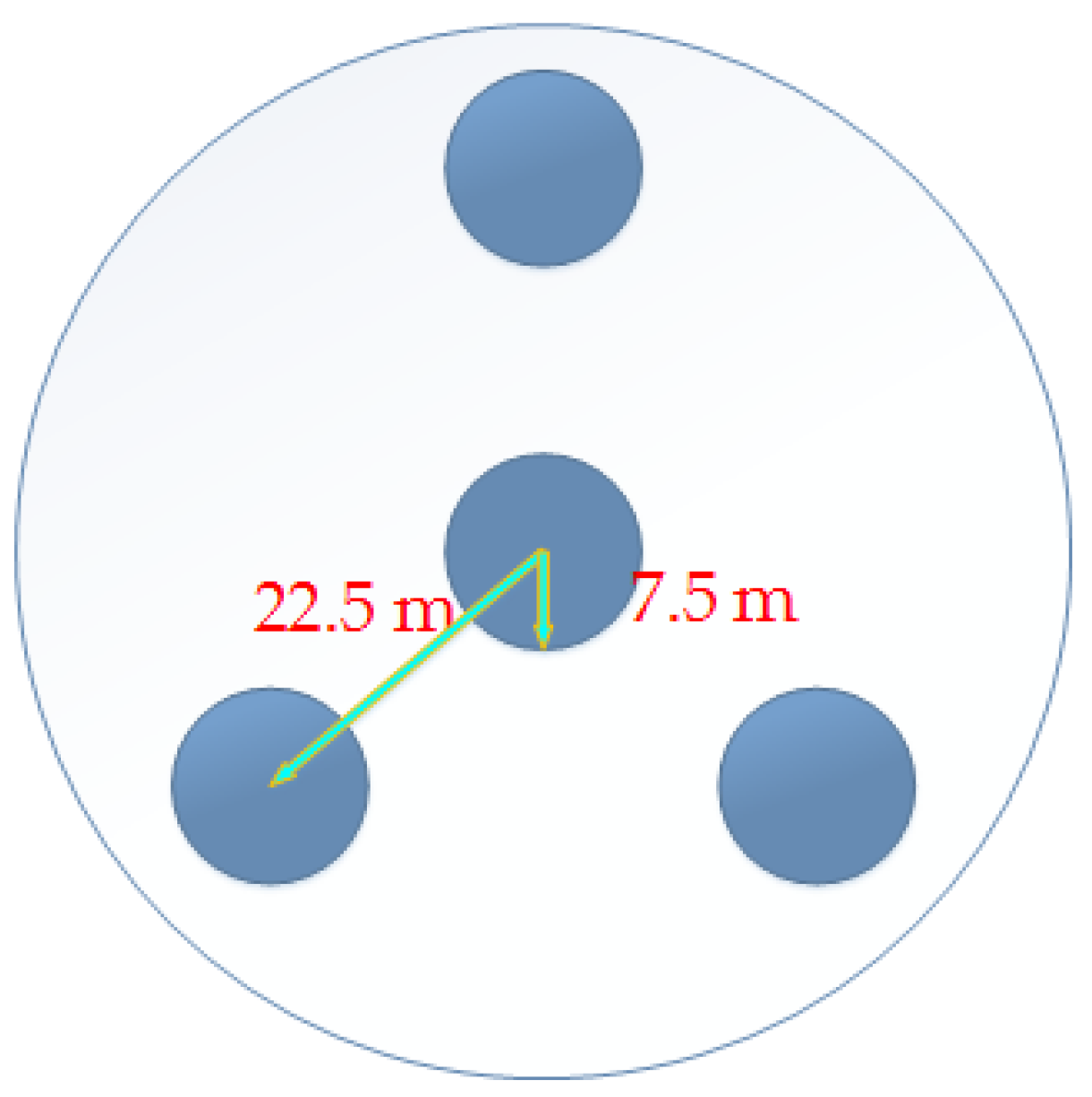
Figure 3.
Model predictions from species-specific allometric equations for aboveground biomass. Different lines represent different tree species.
Figure 3.
Model predictions from species-specific allometric equations for aboveground biomass. Different lines represent different tree species.

Figure 4.
Forest AGB estimation methodology used in this paper.
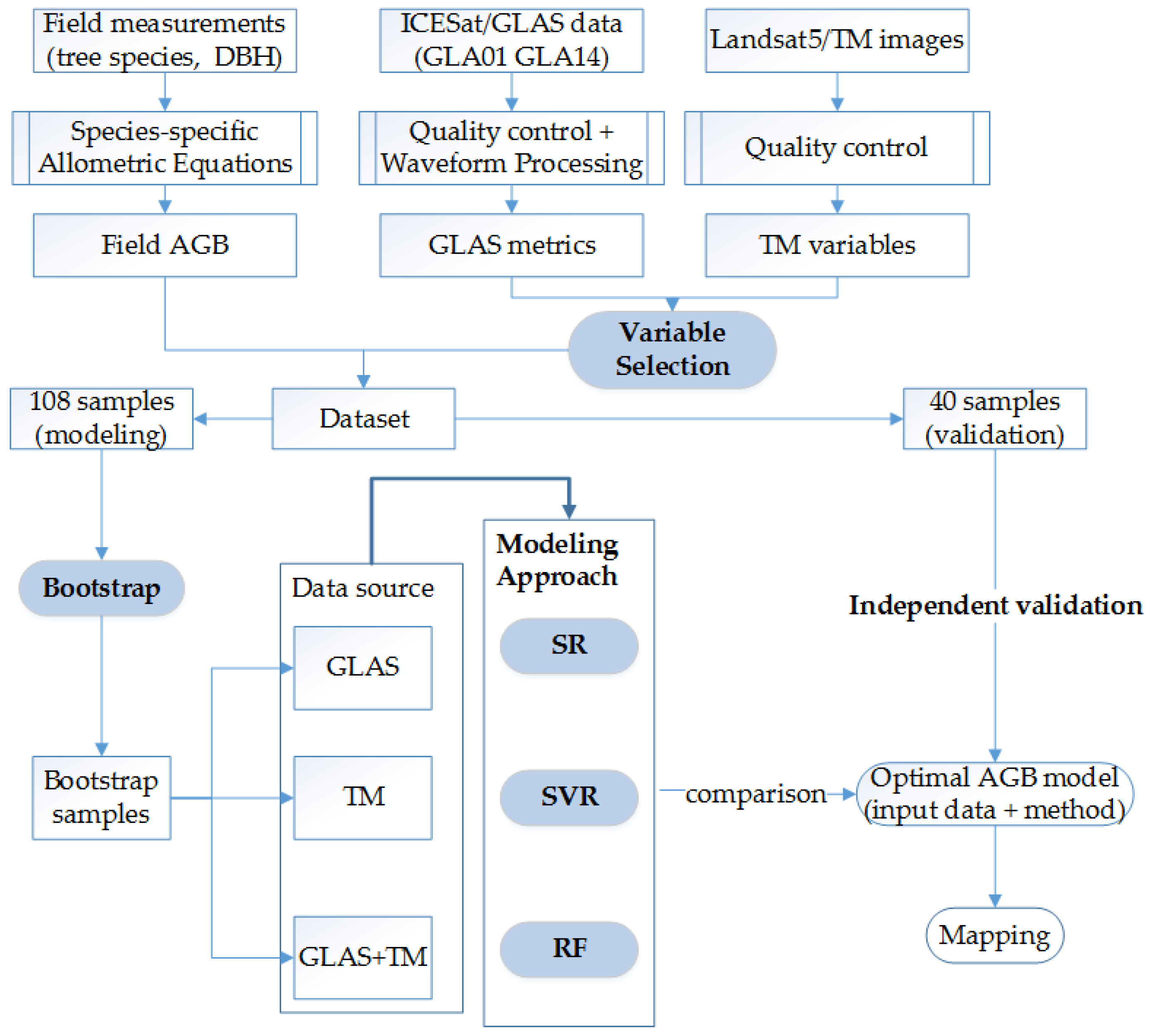
Figure 5.
Flowchart of RF algorithm.
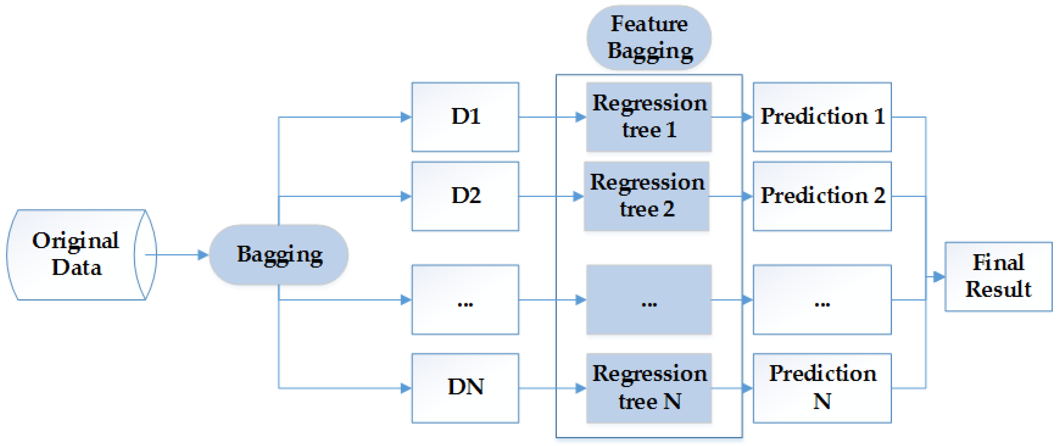
Figure 6.
RMSE, SNR, and r from different filters. The pink lines represent results from the wavelet transform and the blue line represents results from the Gaussian filter. The X-axis (Number) represents the serial number of the 108 GLAS data points.
Figure 6.
RMSE, SNR, and r from different filters. The pink lines represent results from the wavelet transform and the blue line represents results from the Gaussian filter. The X-axis (Number) represents the serial number of the 108 GLAS data points.

Figure 7.
Pearson’s correlation coefficient (r) between the fitted waveforms and the raw waveforms. The red line represents the results from the proposed method, and the black line represents the results from GLA14. The X-axis (Number) represents the serial number of the 108 GLAS data points.
Figure 7.
Pearson’s correlation coefficient (r) between the fitted waveforms and the raw waveforms. The red line represents the results from the proposed method, and the black line represents the results from GLA14. The X-axis (Number) represents the serial number of the 108 GLAS data points.

Figure 8.
Modeling accuracy results from regression using different input data and prediction approaches. The distribution of RMSE and R2 is shown as a violin plot [63], which is the combination of a box plot and a density plot. The white point represents the median, and the black box indicates the interquartile range.
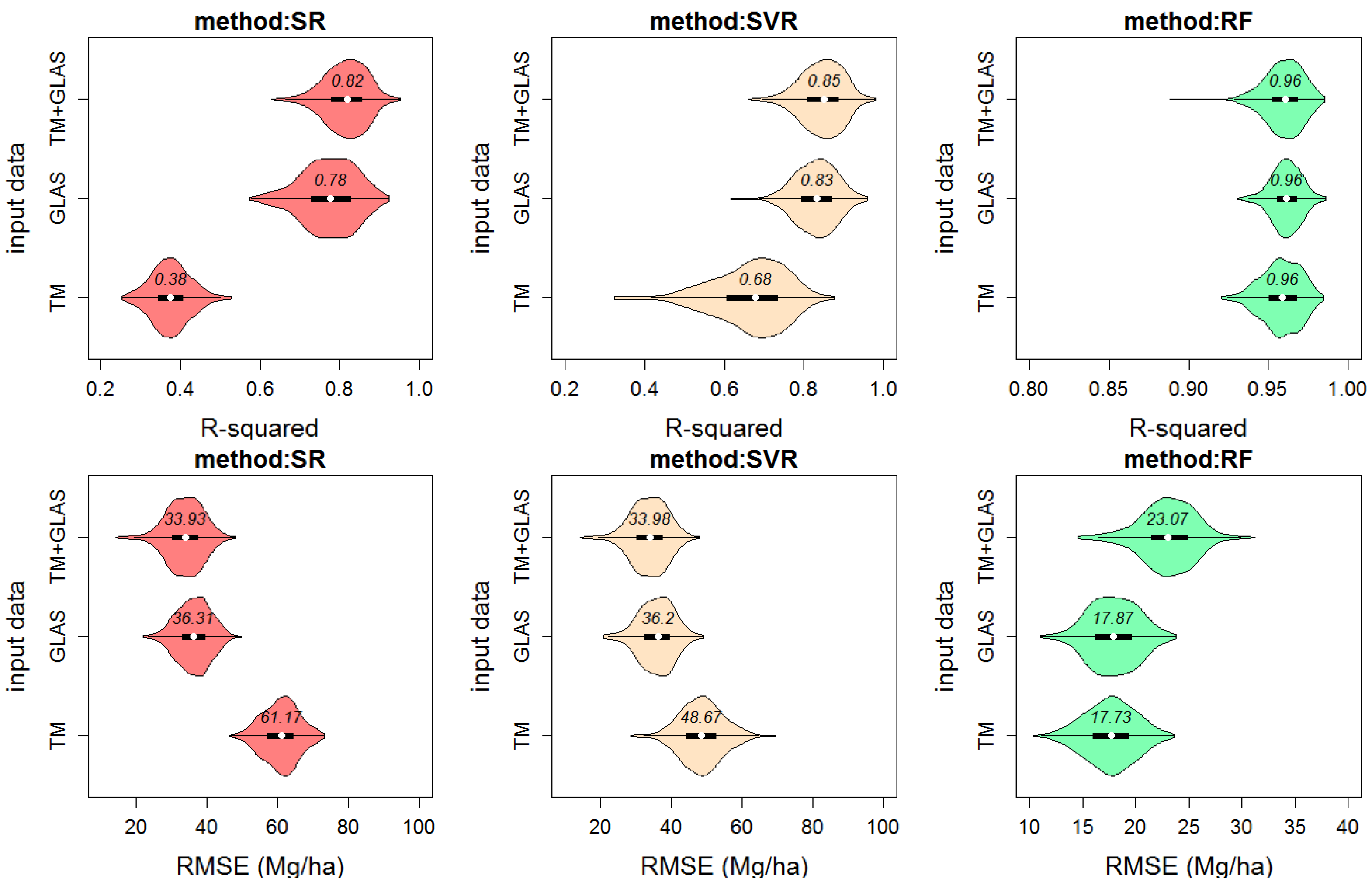
Figure 9.
Results from cross validation using different input data and prediction approaches. The distribution of RMSE and R2 is shown as a violin plot [63].
Figure 9.
Results from cross validation using different input data and prediction approaches. The distribution of RMSE and R2 is shown as a violin plot [63].
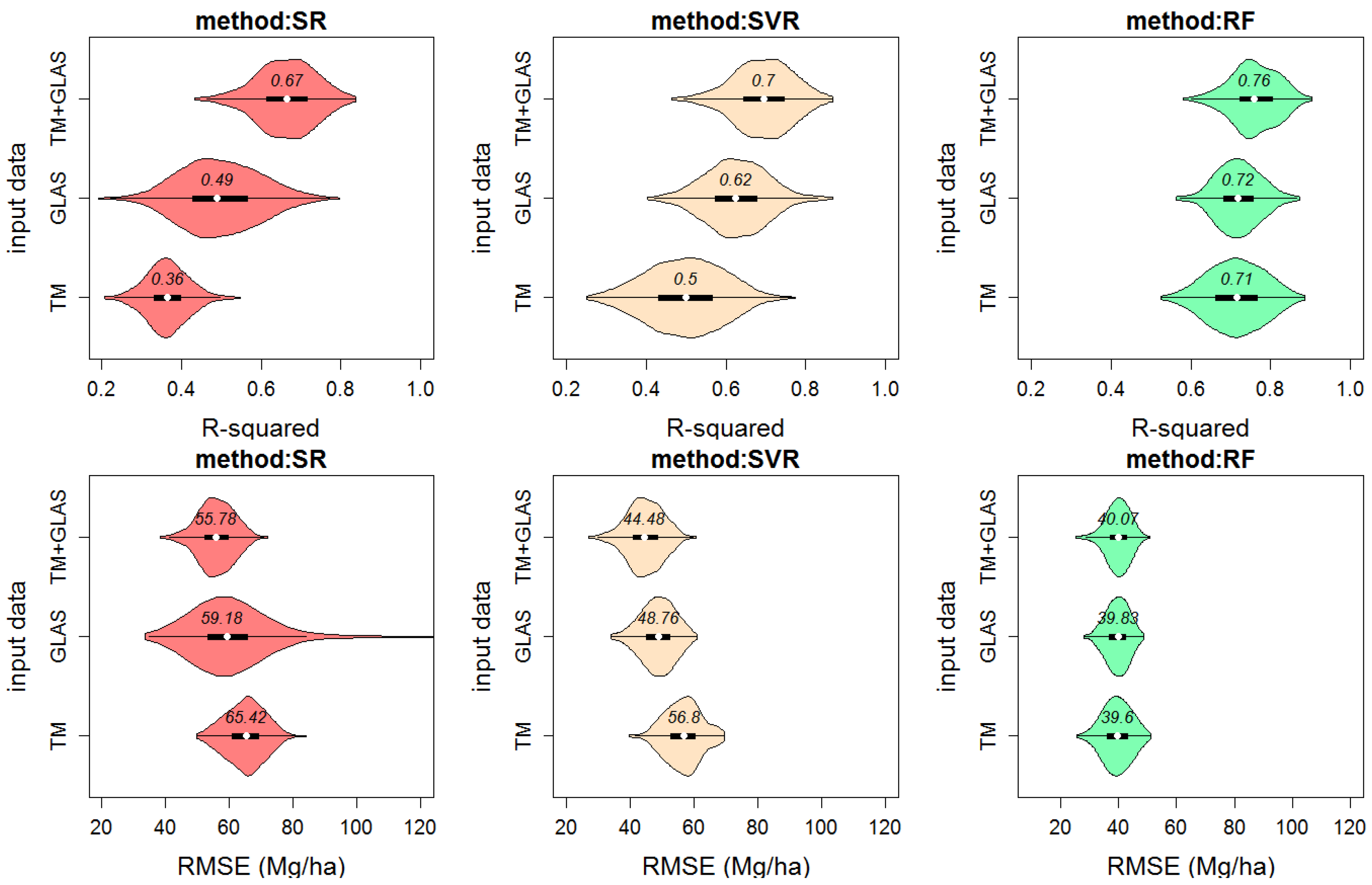
Figure 10.
Predicted AGB vs. field AGB. The size of the point, n, represents the number of repetition points. The color of the point is transparent pink. The black dotted line represents the 1:1 line.
Figure 10.
Predicted AGB vs. field AGB. The size of the point, n, represents the number of repetition points. The color of the point is transparent pink. The black dotted line represents the 1:1 line.
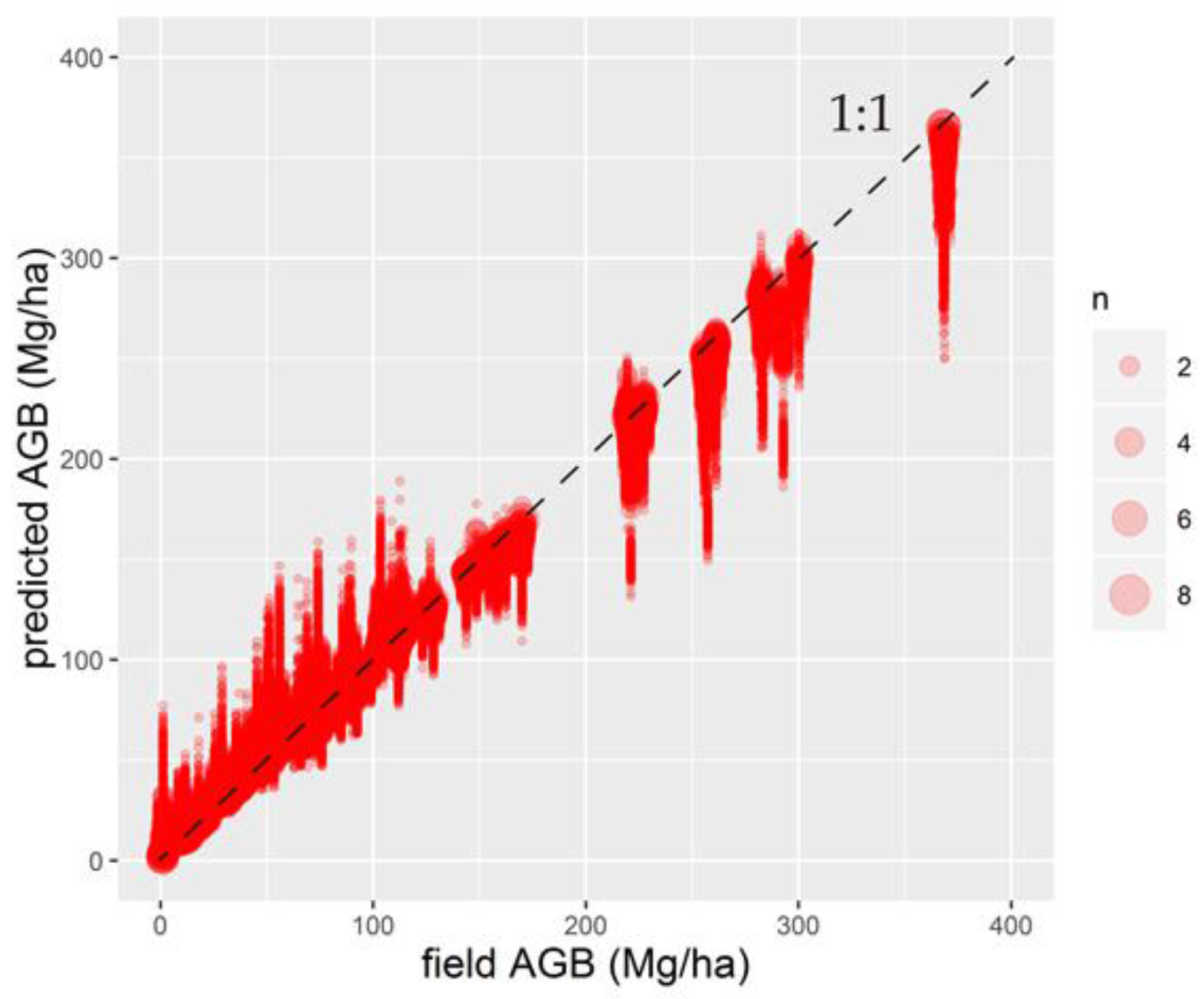
Figure 11.
Modeling accuracy results of regression from different sample size using the RF AGB model. The numbers represent median values.
Figure 11.
Modeling accuracy results of regression from different sample size using the RF AGB model. The numbers represent median values.
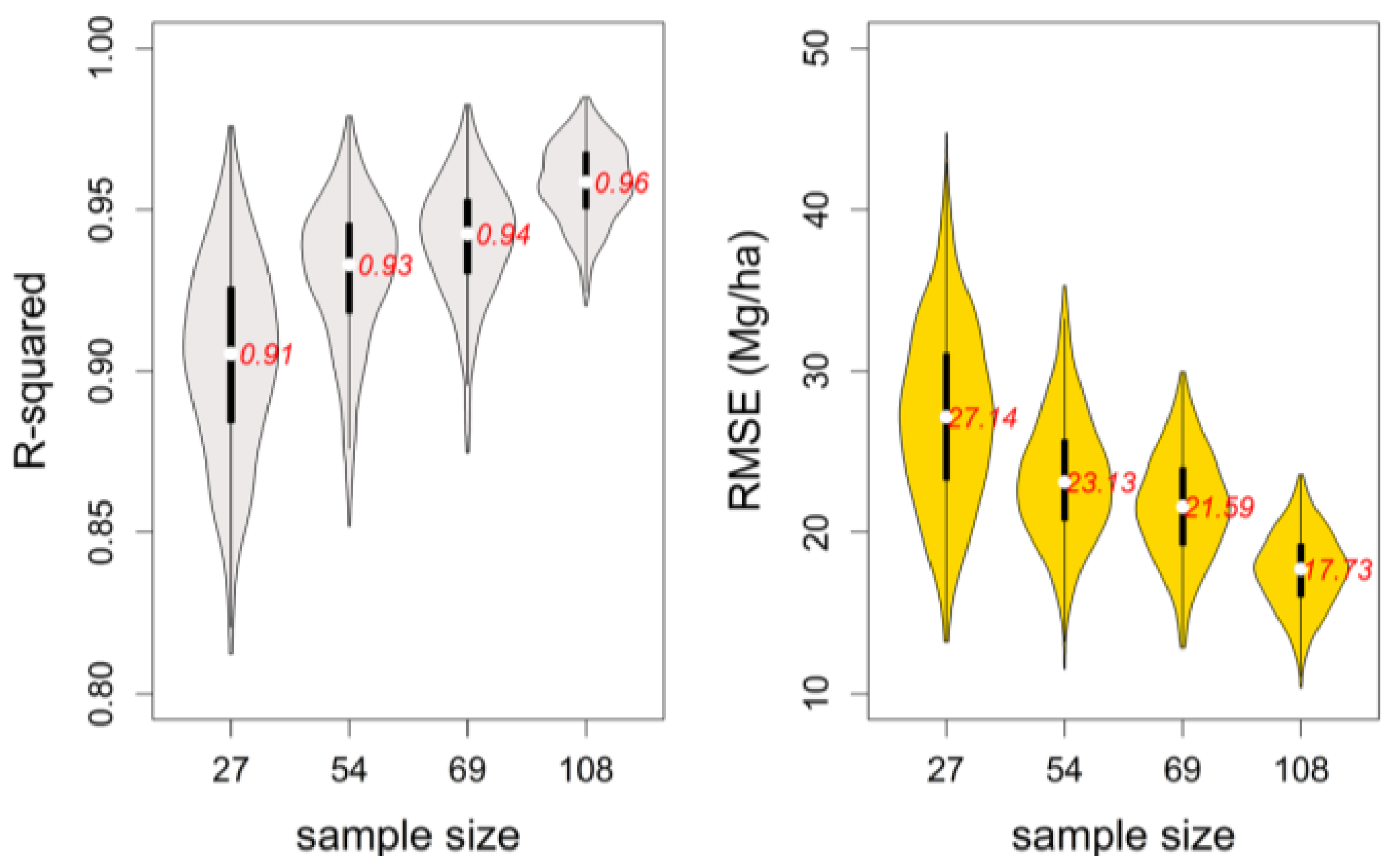
Figure 12.
Modeling accuracy results of regression from RF AGB models with different input data from 69 samples. The numbers represent median values.
Figure 12.
Modeling accuracy results of regression from RF AGB models with different input data from 69 samples. The numbers represent median values.

Figure 13.
Independent validation results from RF AGB model with TM data from 40 datasets. The red dotted line represents the 1:1 line.
Figure 13.
Independent validation results from RF AGB model with TM data from 40 datasets. The red dotted line represents the 1:1 line.
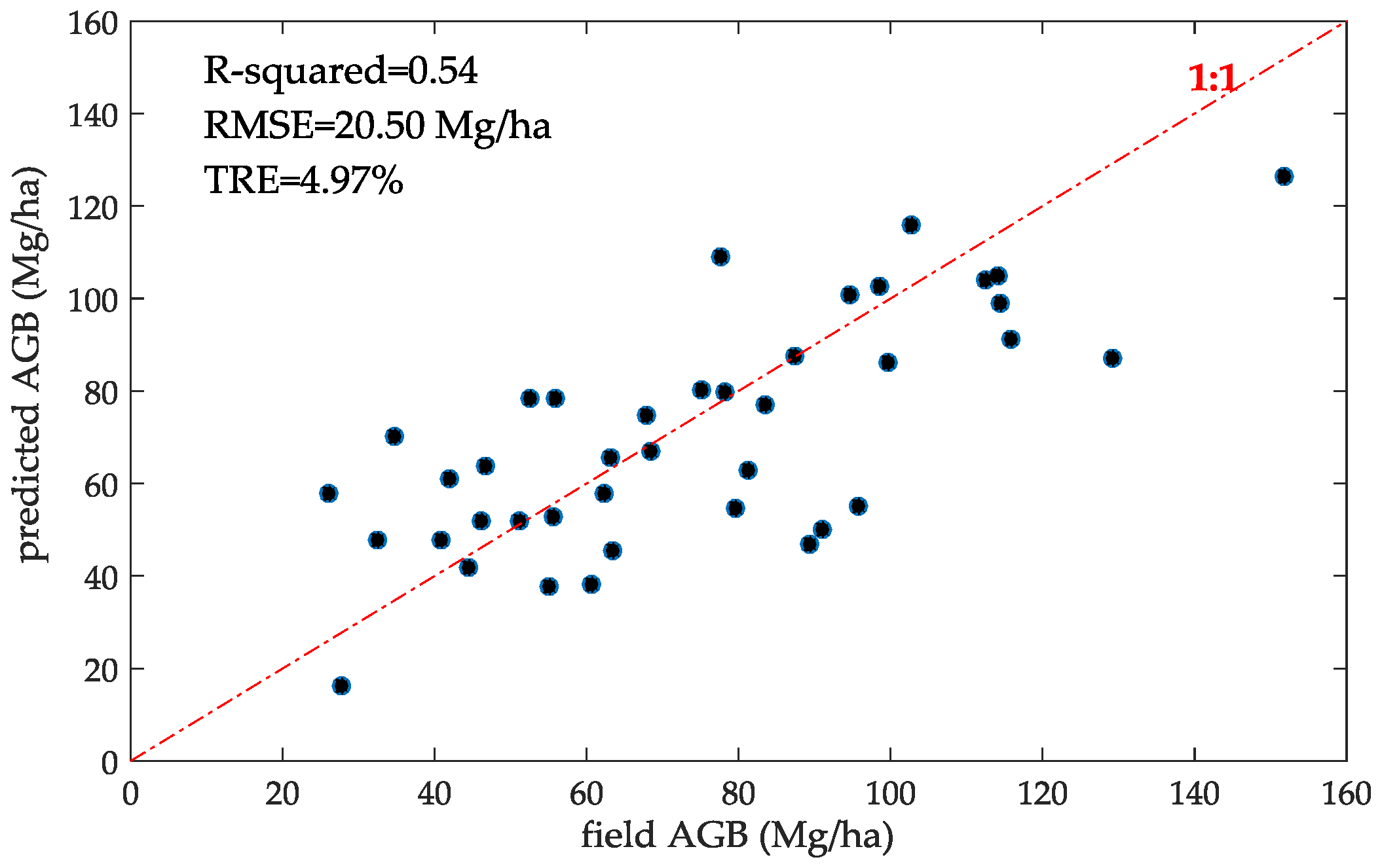
Figure 14.
Forest AGB density map from RF AGB model with TM data over the Daxing’anling Mountains for 2005. The background information is a 30-m forest distribution map developed by Chen [21].
Figure 14.
Forest AGB density map from RF AGB model with TM data over the Daxing’anling Mountains for 2005. The background information is a 30-m forest distribution map developed by Chen [21].


Table 1.
The acquisition time of the materials.
| Data | Acquisition Time | |
|---|---|---|
| Field data | 2005, 2006 and 2007 | |
| GLAS data | L2A | 25 September 2003–19 November 2003 |
| L2D | 25 November 2008–17 December 2008 | |
| L3A | 3 October 2004–8 November 2004 | |
| L3B | 17 February 2005–24 March 2005 | |
| L3C | 20 May 2005–23 June 2005 | |
| L3D | 21 October 2005–24 November 2005 | |
| L3F | 24 May 2006–26 June 2006 | |
| L3G | 25 October 2006–27 November 2006 | |
| Landsat5/TM data | July 2005 | |
Note: L2A, L2D, etc. represent the name of the GALS laser campaigns.
Table 2.
Descriptions and references of GLAS metrics derived from GLAS data.
| Types | GLAS Metric Abbreviations | Descriptions |
|---|---|---|
| The height metrics | Extent | The distance from signal beginning to signal ending [34]. |
| Treeht | The distance from signal beginning to ground peak [34,38]. | |
| Treeht2 Treeht3 | Top tree heights with corrections [34]. | |
| H25 H75 | Quartile heights calculated by subtracting the ground elevation from elevation at which 25% or 75% of the returned energy occurs [34,39]. | |
| H10 H20 H100 | Decimal heights calculated by subtracting the ground elevation from elevation at which 10% (20%...100%) of the returned energy occurs [34]. | |
| LEE | The distance from the elevation of signal beginning to the first elevation at which the signal strength of the waveform is half of the maximum signal [38]. | |
| TEE | The distance from the last elevation at which the signal strength of the waveform is half of the maximum signal to the elevation of signal ending [38]. | |
| HOME | The height of median energy (HOME) [9]. | |
| Meanh Medh | Mean canopy height, median canopy height [40]. | |
| QMCH | Quadratic mean canopy height (QMCH) calculated from the canopy height profiles [40]. | |
| The intensity metrics | Canopy cover | The ratio of the canopy echo area to the total wave area [41]. |
| AVAW | The area under the waveform from vegetation [41]. |
Table 3.
Spectral variables derived from Landsat5/TM data.
| Spectral Variables | Formula |
|---|---|
| NDVI | |
| EVI | |
| PVI | |
| SAVI | |
| NDIIB6 | |
| NDIIB7 | |
| TCB | |
| TCG | |
| TCW | |
| TCdistance | |
| TCangle |
Note:
.
Table 4.
Mean values of RMSE, SNR, and r from different filters.
| Method | RMSE | SNR(dB) | r |
|---|---|---|---|
| wavelet transform | 0.73 | 35.67 | 0.53 |
| Gaussian filter | 1.02 | 33.15 | 0.54 |
© 2017 by the authors. Licensee MDPI, Basel, Switzerland. This article is an open access article distributed under the terms and conditions of the Creative Commons Attribution (CC BY) license (http://creativecommons.org/licenses/by/4.0/).
Share and Cite
MDPI and ACS Style
Liu, K.; Wang, J.; Zeng, W.; Song, J. Comparison and Evaluation of Three Methods for Estimating Forest above Ground Biomass Using TM and GLAS Data. Remote Sens. 2017, 9, 341. https://doi.org/10.3390/rs9040341
AMA Style
Liu K, Wang J, Zeng W, Song J. Comparison and Evaluation of Three Methods for Estimating Forest above Ground Biomass Using TM and GLAS Data. Remote Sensing. 2017; 9(4):341. https://doi.org/10.3390/rs9040341
Chicago/Turabian StyleLiu, Kaili, Jindi Wang, Weisheng Zeng, and Jinling Song. 2017. "Comparison and Evaluation of Three Methods for Estimating Forest above Ground Biomass Using TM and GLAS Data" Remote Sensing 9, no. 4: 341. https://doi.org/10.3390/rs9040341
Note that from the first issue of 2016, this journal uses article numbers instead of page numbers. See further details here.