
A Knowledge-Based Search Strategy for Optimally Structuring the Terrain Dependent Rational Function Models


Faculty of Geodesy and Geomatics, K. N. Toosi University of Technology, Tehran 19667-15433, Iran
*
Author to whom correspondence should be addressed.
Remote Sens. 2017, 9(4), 345; https://doi.org/10.3390/rs9040345
Submission received: 19 January 2017
/
Revised: 19 March 2017
/
Accepted: 30 March 2017
/
Published: 11 April 2017
Abstract
:Identifying the optimal structure of terrain dependent Rational Function Models (RFMs) not only decreases the number of Ground Control Points (GCPs) required, but also increases the accuracy of the model, by reducing the multi-collinearity of Rational Polynomials Coefficients (RPCs) and avoiding the ill-posed problem. Global optimization algorithms such as Genetic Algorithm (GA), evaluate the different combinations of parameters effectively. Therefore, they have a high ability to detect the optimal structure of RFMs. However, one drawback of these algorithms is their high computation cost. This article proposes a knowledge-based search strategy to overcome this deficiency. The backbone of the proposed method relies on the technical knowledge about the geometric condition of image at the time of acquisition, as well as the effect of external factors such as terrain relief on the image. This method was evaluated on four different datasets, including a SPOT-1A, a SPOT-1B, an IKONOS-Geo image, and a GeoEye-Geo imagery, using various number of GCPs. Experimental results demonstrate the efficiency of the proposed method to achieve a sub-pixel accuracy using few GCPs (only 4–6 points) in all datasets. The results also indicate that the proposed method improves the computation speed by 140 times when comparing with GA.

1. Introduction
Due to periodical imaging from the earth, satellite sensors have become a powerful and unique tool for multi-temporal analysis. Accurate image geo-referencing is an important pre-processing step for this analysis [1], in order to avoid errors due to misregistration [2], because, even small geometric errors could have a significant effect on retrieval of subsequent information [3]. Most modern satellite imagery is supplied with a sufficient and reliable Rational Polynomial Coefficients (RPC) [4], and sub-pixel geo-referencing accuracies can be achieved by bias-compensating these coefficients using a few Ground Control Points (GCP) [5,6]. However, old archive imagery are a main part of the data sources for multi-temporal analysis. RPCs have not been available for these imagery, and if we could find any, they would not be reliable. Therefore, the Rational Function Model (RFM) can only be applied to the old archive imagery in a terrain dependent manner. However, if an accurately geo-referenced master image is available for the region of interest, old archive imagery can be co-registered with the master image [7].
Despite the popularity and multiple achievements of terrain independent RFMs and their widespread use for high resolution satellite images, the terrain dependent RFMs were not really welcomed [8,9,10]. At least, this can be due to two main reasons: (1) Third-order 3D RFMs encompass 80 parameters [11], none of which are totally independent [12,13]. The existing correlation among these parameters causes the problem be ill-posed [13,14]. This, in turn, results in a steady fall in accuracy and reliability, and, in some cases, even solving the equation system might be impossible [15]. (2) Even if the zero-order term of polynomials in the denominator of RFMs is supposed to be equal to the fixed value of 1.00, at least 39 Ground Control points (GCPs) are still needed to solve the remaining 78 parameters. Obviously, the degree of freedom would be zero in this case; consequently, the results are not quite reliable [16]. In some resources [17], the number of required GCPs for an accurate and reliable solution of terrain dependent RFMs is mentioned as the twice of the minimum sufficient GCPs, i.e., 78 points. In many cases, not only this many control points, but also occasionally the minimum required GCPs are not available either. Thus, some researchers restricted the use of terrain dependent RFMs only to the usages where accuracy is not a major concern [17,18,19], and some others are totally against its utilization [5,9].
There are two main strategies to encounter the ill-posed problems [20]: (1) variational regularization; and (2) variable selection. Regularization of the normal equation plays an important role in the reduction of the multi-collinearity of rational polynomial coefficients (RPC) and improving the model’s accuracy. Nevertheless, in this strategy besides the essential parameters a set of unnecessary ones are estimated as well. In fact, this strategy is attempting to cutting down the negative effect of the inessential parameters on estimating the effectual ones as much as possible. However, unwanted parameters will exist in the model and some GCPs are required to estimate them as well, which indicates an inefficient use of the available GCPs. Conversely, in the second strategy, the unnecessary parameters are put aside; consequently, apart from solving the problem of the ill-posed normal equation, the number of existing unknown parameters will be reduced [12,21,22]. Thus, fewer GCPs are required to solve the model, and, due to the increase in the degree of freedom, the final results will be more reliable [12,22,23]. Moreover, owing to the absence of unnecessary parameters and reducing the multiple correlations between the remaining parameters, the final model would be more interpretable [20].
The main issue in this strategy is to determine the optimal structure of the model through distinguishing the effectual and unnecessary parameters. The strategy accepted in commercial software such as PCI-Geomatica [24] for solving terrain dependent RFM is to use similar structure in the RFM. It means that, regardless of the zero-order term in the denominator polynomials, the structure of the four polynomials in the RFM is considered alike, and the maximum possible number of parameters regarding to the available GCPs are employed in all polynomials. Notwithstanding the least possible computational cost, it is evident that, in this strategy, achieving the most accurate results for a given number of GCPs is quite unlikely. Considering that the image space distortions depends not only on the interior and exterior orientation parameters of the imaging system, but also on other factors such as terrain relief [16], doubtlessly, the optimal structure of the RFM would be different for each scene.
Thus far, a wide variety of studies has been conducted in order to identify the optimal structure of RFMs, which generally fall into two main groups: linear algebra-oriented (LAO) and artificial intelligence-oriented (AIO). Among the LAO studies, the detection of the optimal structure of the RFM based on correlation analysis [21], eigenvalue of structure matrix [5], scatter matrix [25], multi-collinearity analysis [26], and nested regression [20] can be mentioned; and, from the AIO researches, the use of GA [22], modified GA [12], and PSO algorithm [23] to identify the optimal structure of the RFM can be pointed out.
One of the common features of the LAO methods is the sequential choice of parameters. This means that the quality of a parameter is firstly evaluated and its presence in the final structure is decided, then the next parameter is considered. In this way, not all the possible combinations of the parameters are taken into account; and consequently, the final structure would largely depend on the order of the evaluation of the parameters. Thus, the recognized optimal structure would probably not be global because variable selection is a non-deterministic polynomial (NP) problem whose search space is very large [27]. Alternatively, the AIO methods effectively investigate the different combinations of the parameters through taking advantage of the meta-heuristic search algorithms; therefore, they essentially have a higher potential to achieve the global optimal structure [12,22]. In comparison with the LAO methods, one other privilege of AIO methods is the possibility of determining the optimal structure of the RFM for a desirable number of GCPs. However, the computational cost of these algorithms is excessively high, which is a serious drawback from a practical point of view [20].
This paper relies on the technical knowledge of prevailing geometric conditions on the formation of satellite imagery and the effect of external factors (e.g., terrain relief) on the image. A knowledge-based search strategy is proposed to designate the optimal structure of terrain dependent RFMs in the geo-referencing of satellite imagery. Compared to the previous studies, the major advantage of the proposed method can be sought in establishing a balance among the four elements of accuracy, reliability, flexibility, and computational cost.
2. The Geometry of Linear Pushbroom Imaging
In the linear pushbroom imaging, by means of a row of detectors, which are arranged in the focal plane of the sensor and across the flight direction, a narrow strip of the object space is recorded at every instant, Figure 1. With the sensor’s moving forward, consecutive strips of the object space are recorded one after another; thus, its thorough coverage is provided [16].
In this way, the imaging geometry is parallel along the trajectory of linear pushbroom sensors [28]. Considering the rather short acquisition time of the imagery (for example, about 1 s for an IKONOS scene), the velocity, and orientation of the sensor can be assumed constant during the capture of the scene [29,30,31,32]. Hence, modeling the along-track image component via the 3D affine model is easy [32,33,34]. Implicit in the model are two individual projections, one scaled-orthogonal, and the other skew-parallel (Figure 2a). If the angle of the velocity vector and the optical axis of the sensor changes during the acquisition time, a series of time-dependent terms are required to be added to the 3D affine model [28,35]. Eventually, if the position of all ground points is transferred to a common height plane in the object space, the eight-term model can be effectively reduced to six parameters [36,37], which, is the case for images with few terrain reliefs. However, if the terrain relief is considerable, it is essential to provide a 3D affine model with one or more quadratic terms [28].
3. Rational Function Model
In the RFM, the relationship of image space components (r,c) is stated according to the division of two 3D polynomials in object space components (X,Y,Z) [40].To reduce the computational errors and to improve the numerical stability of the equations, image and object coordinates are both normalized to the range of −1.00 to +1.00 [11]. The direct RFM is given in Equation (1) [40]:
where r and c are row and column components of the image space, respectively; X, Y, and Z are the points’ coordinates in the object space; and Pi is a polynomial in the ground coordinates. The maximum power of each ground coordinate is usually limited to 3, as well as the total power of all ground coordinates [14].
In such a case, each polynomial is of 20-terms cubic form (Equation (2)):
where aijk stands for the polynomial coefficients called rational polynomial coefficients (RPCs). The order of the terms is trivial and may differ in different literature. The above order is adopted from [11].
The distortions caused by the projection geometry can be represented by the ratios of the first-order terms (refer to Section 2), while corrections such as earth curvature, atmospheric refraction, lens distortion, etc., can be well approximated by the second-order terms [14,41]. Significant high-frequency dynamic changes in sensor acceleration and orientation, coupled with large rotation angles, are the main reasons for implementing the third-order and even higher order terms. Fortunately, the relatively smooth trajectory of space borne sensors coupled with the narrow-angle viewing optics, means that such influences are unlikely to be encountered [5].
There are two different computational scenarios for RFMs. If the physical sensor model is available, an approximation of the model could be provided by RFMs; which is a terrain-independent solution and can be used as the replacement sensor model. On the other hand, in the terrain-dependent approach, the unknown parameters of RFMs are estimated using a set of GCPs [14,17,42].
In the terrain-dependent scenario, it is common to consider the zero-order parameter of the denominator polynomials be equal to the fixed value of 1.00, in order to avoid the singularity of the normal equation matrix [5]. Therefore, the model’s parameters decrease to 78 and, to solve them, at least 39 GCPs would be required. When the number of available GCPs is less than the limit, some parameters must be set aside. In the conventional term selection method, the model is estimated with the maximum possible number of parameters. In this way, parameters are included in a sequential manner, while a similar structure (with the exception of the zero-order term of denominator polynomials) is assumed for all polynomials, as it is implemented in PCI-Geomatica software [24]. Therefore, in order to use up “n” parameters in the structure of each polynomial, “2 × n − 1” GCPs are required to solve the RFM.
4. Proposed Method
According to Section 2 and Section 3, it can be noted that the first-order terms of the RFM play the most important role in the modeling of the image space distortions. In the vendor-provided RPCs, the coefficient of the zero- and first-order terms in both the numerator and the denominator polynomials are larger by many orders of magnitude than those of the second- and third-order terms [14], which in fact refers to the same thing. In the case of limited available GCPs, the relative priority of compeer terms depends on the conditions of the scene being modeled. Regarding the different geometry of the along-track and the across-track components, the number of required parameters in the two denominator polynomials is different. Moreover, increasing the field of view of the sensor leads to one or more second-order terms that is required in order to model the earth curvature, the off-nadir viewing angle of the sensor, and the lens distortion effects. The utilization of the third-order terms in the model’s structure depends on the availability of the sufficient GCPs. Accordingly, the following search strategy is proposed for a given number of available GCPs. In the first step, a simplified version of the RFM is considered as Equation (3).
where (X,Y,Z) are the object space coordinates; (r,c) are the image space coordinates; ai, bi, ci, and di are the unknown coefficients of the model; P1 and P3 are the numerator polynomials of the row and column components; and P2 and P4 are the denominator polynomials of the row and column components, respectively.
Since the zero-order term of the numerator polynomials has an effective contribution, this term is used for both the row and the column components in the final structure of the RFM. All possible combinations of the remaining 12 parameters in the structure of Equation (3) are evaluated separately for each of the row and the column components and the optimal structure of the RFM are detected. The search space of the first step is illustrated in Figure 3.
In the first step, the maximum number of the search cases is equal to 4095, which can be calculated using Equation (4).
where N1 is the maximum number of the search cases in the first step of the proposed method.
Thereafter, the necessary first- and second-order terms are determined. In the second step, the feasibility of the enrichment of the detected structure is evaluated by means of adding the third-order terms to the numerator polynomials. Therefore, the functional form of the RFM being searched would be as Equation (5).
where {Piopt} is the optimal structure of the i-th (for i = 1, 2, 3, and 4) polynomial of Equation (3), which is detected in the first step.
Afterwards, all possible combinations of these 10 added third-order terms to the numerator polynomials are searched in the presence of the optimal structures form the first step. Search space of the second step is illustrated in Figure 4.
In the second step, the maximum number of the search cases is equal to 1050, which can be calculated from Equation (6).
where N2 is the maximum number of the search cases in the second step of the proposed method.
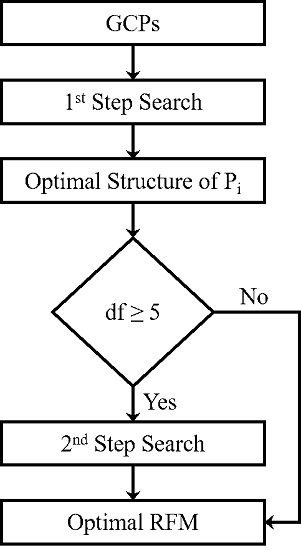
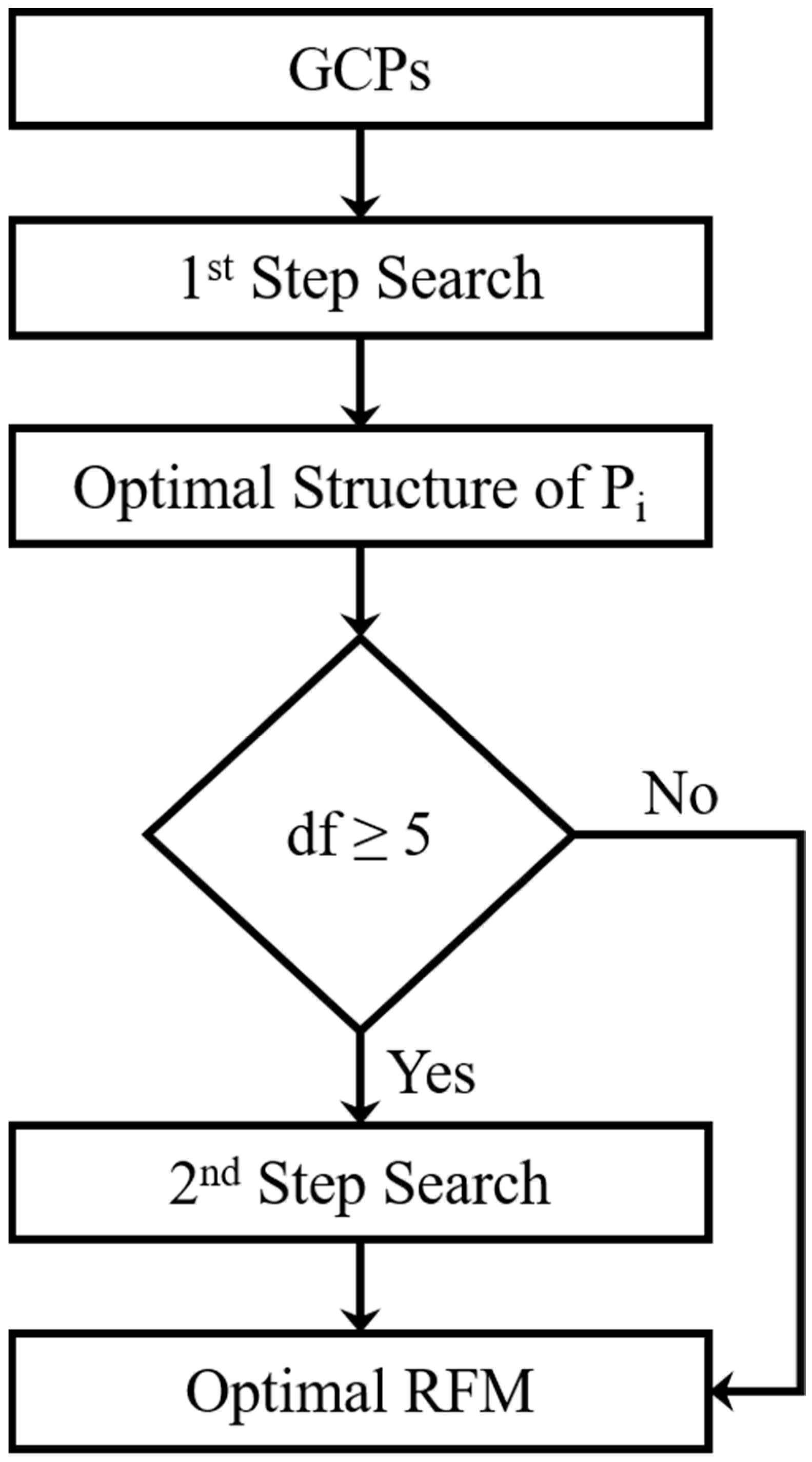
Obviously, the feasibility of executing the second step search depends on the number of available GCPs and the number of terms of the optimal structures from the first step. According to repetitive experiments, it is suggested that only if the first step had been completed with at least five degrees of freedom (df), the second step to be executed. Thus, the flowchart of the proposed method would be as in Figure 5.
In this paper, the Goodness-of-Fit (GoF) of the created model for each structure to be searched was used to detect the optimal structure of RFM [20]. GoF of a statistical model describes how well the model fits a set of observations [43]. The coefficient of determination of a linear regression between the observed and estimated values is used as the statistical measure of GoF, Equation (7).
where n is the number of observation, is the i-th observation value, is the mean of all the observation values, and is the regression result of the i-th observation. The value of R2 is in the range of 0 to 1. The greater the value of R2 is, the better the regression line approximates the observation data, and the more suitable the model [44].
In addition to R2, the degree of freedom of the created model was considered as a measure of the internal reliability of the model. Thus, the final benefit function for assessing different structures in the proposed search scheme can be written as Equation (8), which has to be maximized.
where is the determination coefficient of j-th structure (Sj), dfj is the degree of freedom of the Sj, and B(Sj) is the benefit factor of the Si.
5. Data Used
Four different datasets in Iran have been used in this article, including a SPOT-1A and a SPOT-1B imagery over Isfahan city, an IKONOS-Geo image, and one GeoEye-Geo image covering Hamedan and Uromieh cities, respectively. SPOT-3 Level lA is raw data that have been corrected radiometrically, while Level 1B data has been corrected additionally for certain known geometric distortions (Earth rotation and curvature, mirror look angles and orbit characteristics). Thus, SPOT-3 Level 1B image is partially rectified and approximates to an orthographic view of the Earth, but with the displacements due to relief remaining in the image. Furthermore, in this level, after these geometric corrections have been applied, the image is resampled at regular intervals of 10 m [16]. To produce a Geo product, Ikonos-2 and GeoEye-1 images use a correction process that removes image distortions introduced by the collection geometry and then resamples the imagery to a uniform ground sample distance and a specified map projection. Geometric information and the number of available GCPs of each dataset are shown in Table 1, along with the elevation relief of each dataset.
GCPs for Isfahan dataset were measured, in 1996, using differential GPS techniques based on the use of 3 Ashtech 12 dual frequency GPS sets. The accuracy of these points is estimated to be of the order of sub-meters. Their corresponding image co-ordinates were measured with an approximate precision of 0.5 pixels. For Hamedan and Uromieh datasets, GCPs were extracted from 1:2000 scale digital topographic maps produced by the National Cartographic Center (NCC) of Iran with 0.6 m planimetric and 0.5 m altimetric accuracies, respectively. The points are distinct features such as buildings, pool corners, walls, and road junctions. Their corresponding image coordinates were measured with an approximate precision of one pixel. These accuracies are lower than the potentially achievable accuracies from GeoEye-1 imagery. However, no better ground information was available for this dataset.
6. Results
In order to evaluate the accuracy of the proposed method, as it is impacted by the number of utilized GCPs, several experiments were performed on each dataset used. In each test, the root mean square error (rmse) of independent check points (CP), the mean, standard deviation (std.), and maximum absolute (max.) of residuals across the image’s rows (δr) and columns (δc), the condition number of the normal equation matrix (cond), the number of coefficients in P1, P2, P3, and P4 polynomials, and the degree of freedom (df) of the equation system are provided in Table 2, Table 3, Table 4 and Table 5, for both the first and the second steps.
As can be seen from the results given in Table 2, Table 3, Table 4 and Table 5, the method is able to achieve sub-pixel accuracies even if a few GCPs (i.e., only 4–6 points) are available. In addition, the results of the proposed method are robust with respect to the number and combination of ground control points, and by changing the number of control points, there were no significant changes in the results. The comparison can be made with the results obtained with the conventional RFM and optimally structured RFM using GA [22], which are given in Table 6, Table 7, Table 8 and Table 9. For a fair comparison, number and combination of GCPs were adopted similar to those of Table 2, Table 3, Table 4 and Table 5. The GA, however, did not converge to an acceptable result for fewer than eight GCPs in all datasets. Therefore, these results were excluded from Table 6, Table 7, Table 8 and Table 9. For each experiment, the GA was performed 10 times and the best results were reported. The number of parents, the population of generations, and maximum number of iterations were set to 20, 200, and 500, respectively. A detail description of GA optimization of RFMs is available in [22]. Comparisons of the results in Table 2, Table 3, Table 4 and Table 5 with Table 6, Table 7, Table 8 and Table 9 show that accuracies obtained from the proposed method are considerably better than those obtained by conventional RFMs. Although the accuracies form the proposed method are a little better than those obtained by the GA-optimized RFMs, but the proposed algorithm benefits from remarkably higher degrees of freedom leading to more reliable results. In addition, the computational cost of the proposed method is significantly lower than that of GA algorithm, which confirms its effective performance.
In another experiment, low order polynomials (i.e., first and second order polynomials in X, Y, and Z) were utilized for georeferencing the satellite imagery (Table 10, Table 11, Table 12 and Table 13). Normalized image and ground coordinates were used to estimate the models’ coefficients. Again, number and combination of GCPs were adopted similar to those of Table 2, Table 3, Table 4 and Table 5.
According to Table 10, Table 11, Table 12 and Table 13, first-order polynomials could not supply sub-pixel accuracies for SPOT-1A and SPOT-1B images, and the maximum absolute residual errors across the column numbers of Geoeye imagery are greater than one pixel, despite its sub-pixel accuracies. Second-order polynomials could not also provide sub-pixel accuracies for SPOT-1A imagery.
As the final experiment, the accuracy of the proposed method was examined with respect to the RPCs provided with Geoeye imagery. In this regard, first the RPCs were bias-compensated using four GCPs. Then, a regular grid of 100 image points was established, which is called original image points (OIPs) in this paper. Afterwards, these points were projected to the ground space for arbitrary heights in the range of the ground elevations by utilizing the compensated RPCs. Finally, these ground points were back-projected to the image space by means of the optimally structured RFM using the proposed method, which is called computed image points (CIPs). The mean, standard deviation (std.), and maximum absolute (max.) of discrepancies between the OIPs and CIPs across the image’s rows (δr) and columns (δc) are provided in Table 14, along with their root mean square error (rmse).
7. Discussion
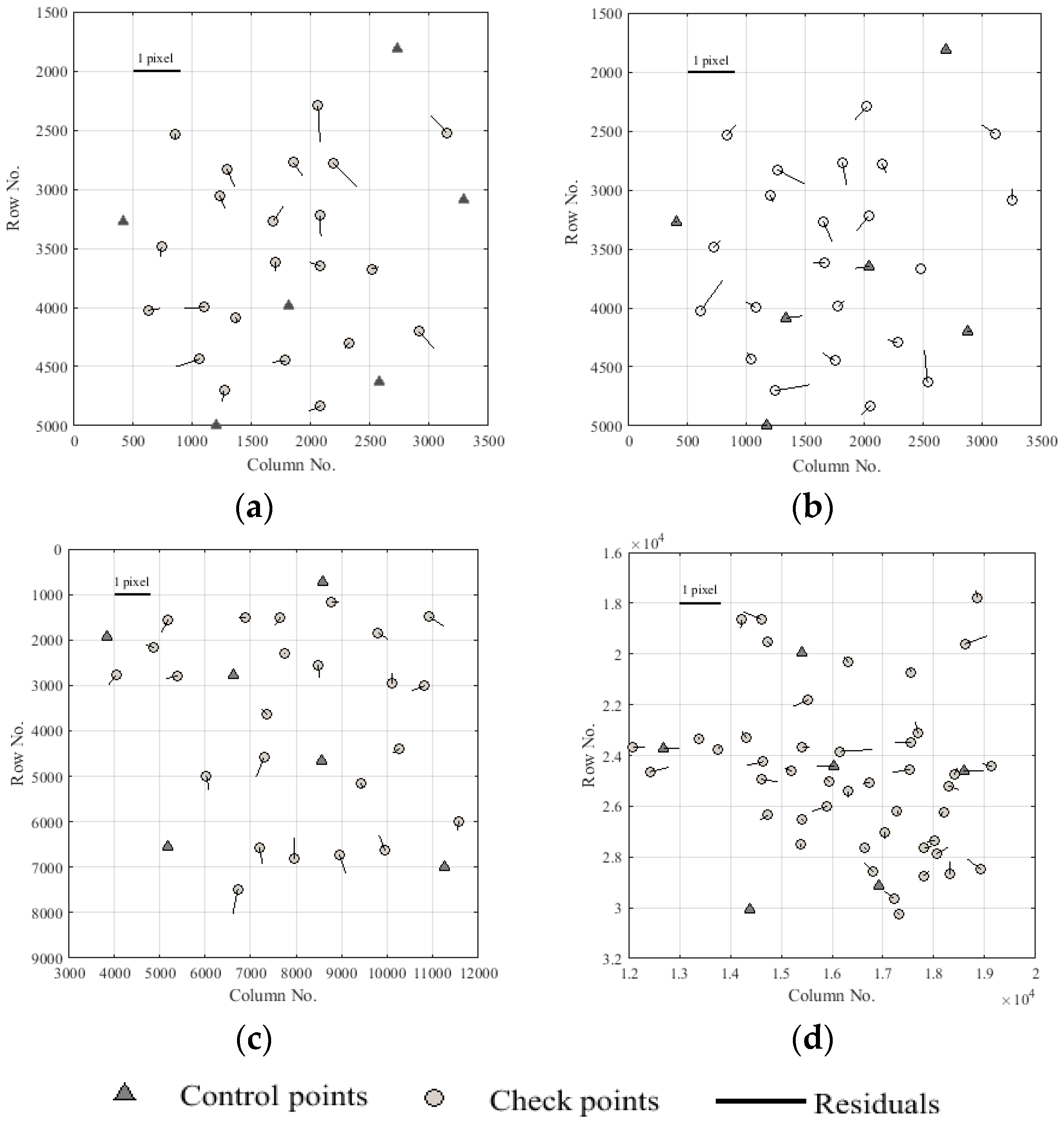
According to Table 2, Table 3, Table 4 and Table 5, the proposed method is able to achieve sub-pixel accuracies even if the number of available GCPs is limited; so that, sub-pixel accuracies were obtained using only six GCPs in all datasets. Scatter plot of residual errors shows that no systematic errors have occurred (Figure 6). Moreover, the results from the proposed method are robust with respect to the number of available GCPs, so that there is no considerable change in the results with changing the number of GCPs. Obtained condition numbers illustrate that the normal equation matrices of the proposed method are pretty well-conditioned.
For the last three datasets (i.e., SPOT-1B, IKONOS-Geo, and GeoEye-Geo) which are geometrically corrected, the proposed method could achieve almost one-pixel accuracies using only four GCPs. However, for the first dataset (i.e., SPOT-1A) that is geometrically raw, it could not achieve an accuracy better than seven pixels using even five GCPs, which indicates more parameters are required in the structure of RFM to modeling the image space’s distortions.
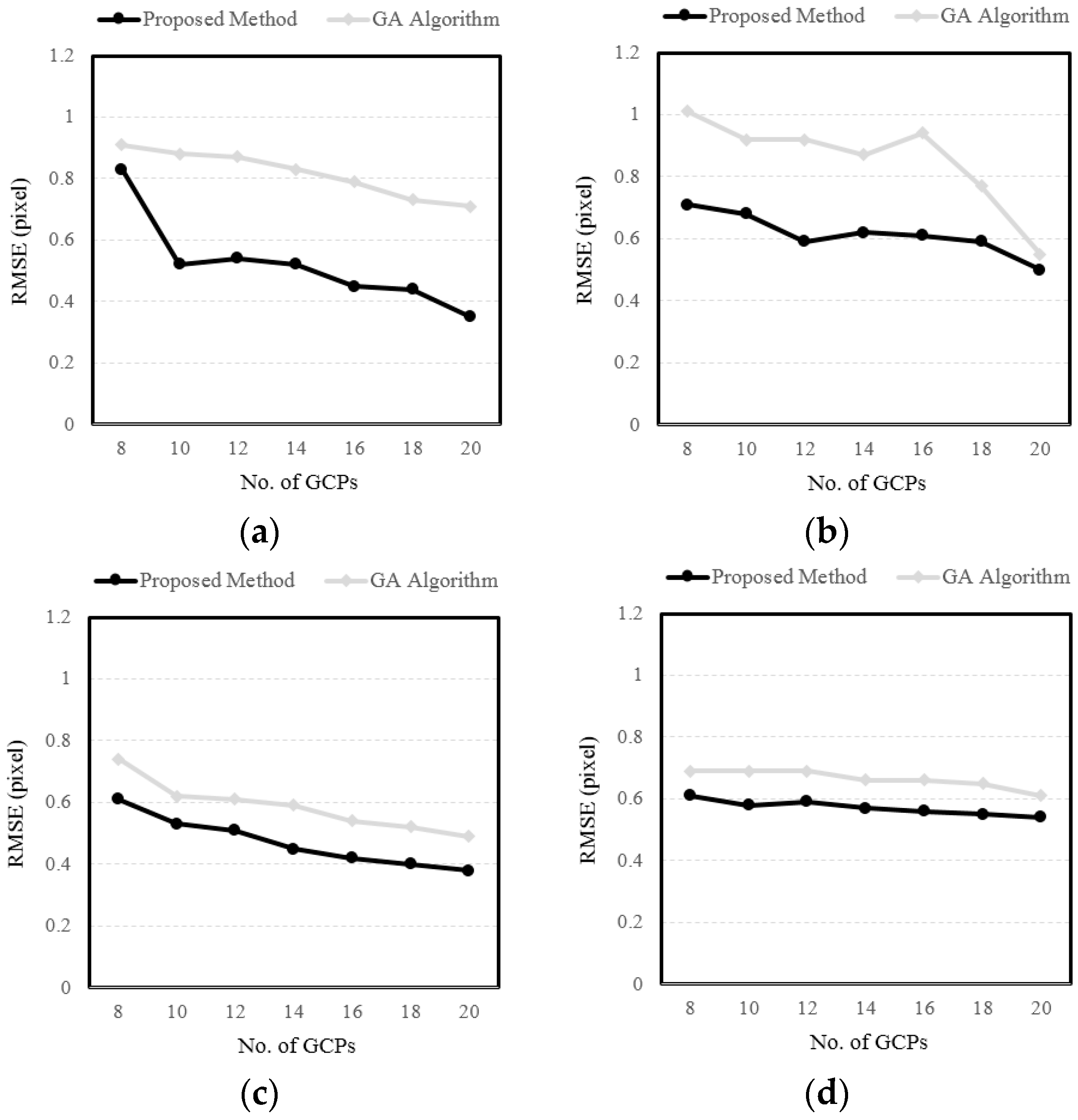
In comparison with the results obtained from GA-optimized RFMs (Table 6, Table 7, Table 8 and Table 9), accuracies of the proposed method are competitive and even slightly better. It is worth mentioning that GA can theoretically provide the most accurate result if no computation limit is considered during the optimization process. However, in practice, some stopping criteria (e.g., a critical value for the fitness function or a certain number of iterations) are always utilized to complete the optimization process, which limits the achievable accuracies in comparison with the theoretical ones. In order to better compare these two methods, their accuracies are graphically displayed in Figure 7.
Considering the capability of the GA to globally search the solution space [45], it can be said that the results from the proposed method are to a great extent close to the global optimal solution. Undoubtedly, the final confirmation of the latter result requires more probing in the future studies. In addition, the proposed method can omit a larger number of parameters compared with the GA-optimized RFMs. Therefore, the optimal RFM has a higher number of degrees of freedom, resulting in a higher accuracy. On the other hand, according to Table 6, Table 7, Table 8 and Table 9, the average number of iterations of the GA was 350 iterations. Bearing in mind the fact that the population of each generation was considered to be 200 individuals, in each run the cost function has been evaluated on average 70,000 times; that is, 14 times slower than the proposed method. It should be noted that the results of the GA-optimized RFMs shown in Table 3 are provided for 10 times execution of the algorithm, which by multiplying these two rates, the computational cost if the GA would increase to 140 times.
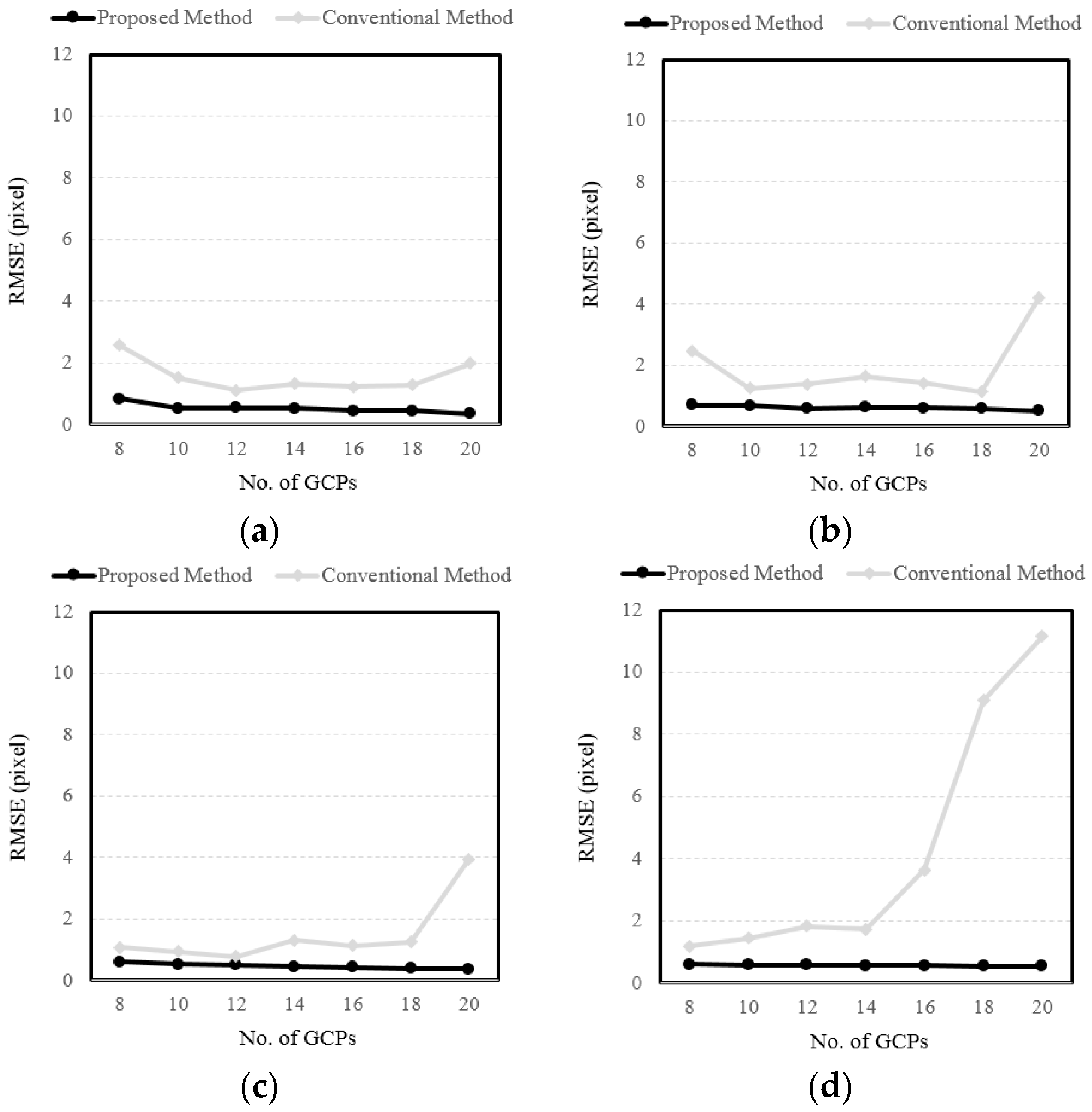
In comparison with the results obtained from the conventional RFMs shown in Table 6, Table 7, Table 8 and Table 9, the proposed method has always achieved better accuracies using fewer parameters. Therefore, the proposed algorithm benefits from higher degrees of freedom leading to more reliable results. Accuracies obtained from these two methods are graphically compared in Figure 8.
According to Figure 8, upon increasing the number of GCPs, the accuracy of conventional RFMs shows an upward trend and after that comes down. It can be noted that increasing the number of GCPs and consequently the number of estimable parameters cover the under-parameterization problem. However, increasing the number of parameters in the model results in the increment risk of the over-parameterization. Consequently, due to the involvement of unnecessary parameters in the model as well as the inherent correlation of some parameters, the overall accuracy of the model will be decreased, whereas this trend is not ever seen in the results of the proposed method, and this method is able to recognize the optimally structured RFMs using any arbitrary number of GCPs.
According to Table 12 and Table 13, first-order polynomials have provided sub-pixel accuracies for Ikonos and Geoeye-1 imagery. This could be due to the fact that these two sensors have a narrow instantaneous field of view (IFOV) and swath width, which leads their geometry to be more similar to a parallel projection. Therefore, a 3D affine model (which is equivalent to a first-order polynomial in X, Y, and Z) is well suited for georeferencing these imagery, as it is confirmed in previous studies [26]. However, it is not the case for sensors with a rather wide IFOV and swath width such as SPOT-3; as the first-order polynomials did not provide sub-pixel accuracies for SPOT-1A and SPOT-1B images.
As the final point, considering the sampling rate and the number of detectors for images used in this research(Table 1), the required time interval to acquire a square scene for SPOT-3, IKONOS and Geoeye-1 sensors are approximately 9, 2 and 3.5 s, respectively. Since the proposed method has provided accurate and reliable results for SPOT-3 imagery, then the proposed method can be well utilized for other sensors with a shorter acquisition time interval.
8. Conclusions
Identifying the optimal structure of terrain dependent RFMs not only decreases the number of required GCPs, but also increases the model’s accuracy through reducing the multi-collinearity of RPCs and avoiding the ill-posed problem. Global optimization algorithms such as GA, evaluate different combinations of the parameters effectively. Thus, they have a high ability to detect the optimal structure of RFMs. However, one drawback of these algorithms is their high computational cost. To address this shortcoming, a knowledge-based search strategy is proposed in this article to identify the optimal structure of terrain dependent RFMs for geo-referencing of satellite imagery. The backbone of the proposed method is relying on the technical knowledge of the conditions controlling acquiring satellite images, as well as the effect of external factors (e.g., terrain relief) on the image space’s distortions. The capability of the proposed method in identifying the optimal structure of RFMs was evaluated, and its results were assessed in comparison with both GA-optimized and conventional RFMs.
According to the results, the proposed method achieved competitive and even better accuracies with a lower computational cost. It is worth mentioning that the speed of two methods was only compared based on the number of times which the cost function has been evaluated, while the search mechanism of the proposed method is much simpler than the GA. Therefore, the proposed method is in reality faster than the aforementioned ratio. Moreover, the proposed method could omit a larger number of parameters. Therefore, the proposed algorithm benefits from higher degrees of freedom leading to more reliable results. Future studies will be focused on the orthophoto and DEM generation using an optimally structured RFM based on the proposed method, as well as the epipolar resampling of linear pushbroom imagery.
Author Contributions
All the authors listed contributed equally to the work presented in this paper.
Conflicts of Interest
The authors declare no conflict of interest.
References
- Brook, A.; Ben-Dor, E. Automatic registration of airborne and spaceborne images by topology map matching with SURF processor algorithm. Remote Sens. 2011, 3, 65–82. [Google Scholar] [CrossRef]
- Aksakal, S.K. Geometric accuracy investigations of SEVIRI High Resolution Visible (HRV) Level 1.5 imagery. Remote Sens. 2013, 5, 2475–2491. [Google Scholar] [CrossRef]
- Aksakal, S.K.; Neuhaus, C.; Baltsavias, E.; Schindler, K. Geometric quality analysis of AVHRR orthoimages. Remote Sens. 2015, 7, 3293–3319. [Google Scholar] [CrossRef]
- Wang, M.; Yang, B.; Hu, F.; Zang, X. On-orbit geometric calibration model and its applications for high-resolution optical satellite imagery. Remote Sens. 2014, 6, 4391–4408. [Google Scholar] [CrossRef]
- Fraser, C.S.; Dial, G.; Grodecki, J. Sensor orientation via RPCs. ISPRS J. Photogramm. Remote Sens. 2006, 60, 182–194. [Google Scholar] [CrossRef]
- Pehani, P.; Cotar, K.; Marsetič, A.; Zaletelj, J.; Oštir, K. Automatic geometric processing for very high resolution optical satellite data based on vector roads and orthophotos. Remote Sens. 2016, 8, 343. [Google Scholar] [CrossRef]
- Ayoub, F. Monitoring Morphologic Surface Changes from Aerial and Satellite Imagery, on Earth and Mars. Ph.D. Thesis, Universite Toulouse III Paul Sabatier, Toulouse, France, 2014. [Google Scholar]
- Jannati, M.; Valadan Zoej, M.J.; Mokhtarzade, M. Epipolar resampling of cross-track pushbroom satellite imagery using the rigorous sensor model. Sensors 2017, 17, 129. [Google Scholar] [CrossRef] [PubMed]
- Jacobsen, K. Satellite image orientation. Int. Arch. Photogramm. Remote Sens. Spat. Inf. Sci. 2008, 37, 703–709. [Google Scholar]
- Zhang, H.; Pu, R.; Liu, X. A new image processing procedure integrating PCI-RPC and ArcGIS-Spline tools to improve the orthorectification accuracy of high-resolution satellite imagery. Remote Sens. 2016, 8, 827. [Google Scholar] [CrossRef]
- NIMA (National Imaging and Mapping Agency). The Compendium of Controlled Extensions (CE) for the National Imagery 7kansmission Format (NITF), 2000, Version 2.1. Available online: http://geotiff.maptools.org/STDI-0002_v2.1.pdf (accessed on 19 January 2017).
- Jannati, M.; Valadan Zoej, M.J. Introducing genetic modification concept to optimize rational function models (RFMs) for georeferencing of satellite imagery. GISci. Remote Sens. 2015, 52, 510–525. [Google Scholar] [CrossRef]
- Long, T.; Jiao, W.; He, G. RPC estimation via L1-Norm-Regularized Least Squares (L1LS). IEEE Trans. Geosci. Remote Sens. 2015, 53, 4554–4567. [Google Scholar] [CrossRef]
- Tao, V.; Hu, Y. A Comprehensive study for rational function model for photogrammetric processing. J. Photogramm. Eng. Remote Sens. 2001, 67, 1347–1357. [Google Scholar]
- Boccardo, P.; Borgogno Mondino, E.; Giulio Tonolo, F.; Lingua, F. Orthorectification of high resolution satellite images. In Proceedings of the XX ISPRS Congress, Istanbul, Turkey, 12–23 July 2004; pp. 30–35. [Google Scholar]
- Valadan Zoej, M.J. Photogrammetric Evaluation of Space Linear Array Imagery for Medium Scale Topographic Mapping. Ph.D. Thesis, University of Glasgow, Glasgow, UK, 1997. [Google Scholar]
- Hu, Y.; Croitoru, A.; Tao, V. Understanding the rational function model: Methods and applications. Int. Arch. Photogramm. Remote Sens. 2004, 20, 663–668. [Google Scholar]
- Toutin, T.; Cheng, P. Demystification of IKONOS. Earth Obs. Mag. 2000, 9, 17–21. [Google Scholar]
- Toutin, T. Comparison of 3D physical and empirical models for generating DSMs from stereo HR images. Photogramm. Eng. Remote Sens. 2006, 72, 597–604. [Google Scholar] [CrossRef]
- Long, T.; Jiao, W.; He, G. Nested regression based optimal selection (NRBOS) of rational polynomial coefficients. Photogramm. Eng. Remote Sens. 2014, 80, 261–269. [Google Scholar]
- Sohn, H.; Park, C.; Yu, H. Application of rational function model to satellite images with the correlation analysis. KSCE J. Civ. Eng. 2003, 7, 585–593. [Google Scholar] [CrossRef]
- Valadan Zoej, M.J.; Mokhtarzade, M.; Mansourian, A.; Ebadi, H.; Sadeghian, S. Rational function optimization using genetic algorithms. Int. J. Appl. Earth Obs. Geoinform. 2007, 9, 403–413. [Google Scholar] [CrossRef]
- Yavari, S.; Valadan Zoej, M.J.; Mohammadzadeh, A.; Mokhtarzade, M. Particle swarm optimization of RFM for georeferencing of satellite images. IEEE Geosci. Remote Sens. Lett. 2012, 10, 135–139. [Google Scholar] [CrossRef]
- PCI Geomatica. PCI Geomatica OrthoEngine User Guide. Available online: https://www.ucalgary.ca/appinst/doc/geomatica_v91/manuals/orthoeng.pdf (accessed on 19 January 2017).
- Zhang, Y.; Lu, Y.; Wang, L.; Huang, X. A new approach on optimization of the rational function model of high-resolution satellite imagery. IEEE Trans. Geosci. Remote Sens. 2012, 50, 2758–2764. [Google Scholar] [CrossRef]
- Yuan, X.; Cao, J. An optimized method for selecting RPCs based on multicolinearity analysis. Geomat. Inf. Sci. Wuhan Univ. 2011, 36, 665–669. [Google Scholar]
- Amaldi, E.; Kann, V. On the approximability of minimizing non-zero variables or unsatisfied relations in linear systems. Theor. Comput. Sci. 1998, 209, 237–260. [Google Scholar] [CrossRef]
- Fraser, C.S.; Yamakawa, T. Insights into the affine model for satellite sensor orientation. ISPRS J. Photogramm. Remote Sens. 2004, 58, 275–288. [Google Scholar] [CrossRef]
- Gupta, R.; Hartley, R.I. Linear pushbroom cameras. IEEE Trans. Pattern Anal. Mach. Intell. 1997, 19, 963–975. [Google Scholar] [CrossRef]
- Wang, Y. Automated triangulation of linear scanner imagery. In Proceedings of the Joint Workshop of ISPRS WG I/1, I/3 and IV/4 on Sensors and Mapping from Space, Hanover, Germany, 27–30 September 1999. [Google Scholar]
- Habib, A.F.; Morgan, M.; Jeong, S.; Kim, K.O. Analysis of epipolar geometry in linear array scanner scenes. Photogramm. Rec. 2005, 20, 27–47. [Google Scholar] [CrossRef]
- Ono, T.; Honmachi, Y.; Ku, S. Epipolar resampling of high resolution satellite imagery. In Proceedings of the Joint Workshop of ISPRS WG I/1, I/3 and IV/4 Sensors and Mapping from Space, Hannover, German, 27–30 September 1999. [Google Scholar]
- Okamoto, A.; Akamatsu, S.; Hasegawa, H. Orientation theory for satellite CCD line-scanner imagery of hilly terrains. Int. Arch. Photogramm. Remote Sens. 1992, 29, 217–222. [Google Scholar]
- Morgan, M. Epipolar Resampling of Linear Array Scanner Scenes. Ph.D. Thesis, University of Calgary, Calgary, AB, Canada, 2004. [Google Scholar]
- Hanley, H.; Yamakawa, T.; Fraser, C. Sensor Orientation for High Resolution Satellite Imagery; ISPRS (International Archives of Photogrammetry Remote Sensing and Spatial Information Sciences): Denver, CO, USA, 2002. [Google Scholar]
- Baltsavias, E.; Pateraki, M.; Zhang, L. Radiometric and geometric evaluation of Ikonos Geo images and their use for 3D building modeling. In Proceedings of the Joint ISPRS Workshop High Resolution Mapping from Space 2001, Hanover, Germany, 19–21 September 2001. [Google Scholar]
- Fraser, C.S.; Baltsavias, E.; Gruen, A. Processing of Ikonos imagery for sub-metre 3D positioning and building extraction. ISPRS J. Photogramm. Remote Sens. 2002, 56, 177–194. [Google Scholar] [CrossRef]
- Kim, T. A study on the epipolarity of linear pushbroom images. Photogramm. Eng. Remote Sens. 2000, 66, 961–966. [Google Scholar]
- Lee, H.Y.; Park, W. A new epipolarity model based on the simplified pushbroom sensor model. Int. Arch. Photogramm. Remote Sens. Spat. Inf. Sci. 2002, 34, 631–636. [Google Scholar]
- OGC (Open GIS Consortium). The Open GIS Abstract Specification—Topic 7: The Earth Imagery Case. Available online: http://www.opengis.org/docs/99-107.pdf (accessed on 19 January 2017).
- Tao, C.V.; Hu, Y. Investigation on the Rational Function Model. In Proceedings of the 2000 ASPRS Annual Convention, Washington, DC, USA, 24–26 May 2000. [Google Scholar]
- Madani, M. Real-Time Sensor-Independent Positioning by Rational Functions. In Proceedings of the ISPRS Workshop on “Direct versus Indirect Methods of Sensor Orientation”, Barcelona, Spain, 25–26 November 1999; pp. 64–75. [Google Scholar]
- Cameron, A.; Windmeijer, F. An r-squared measure of goodness of fit for some common nonlinear regression models. J. Econom. 1997, 77, 329–342. [Google Scholar] [CrossRef]
- Pang, H. Econometrics; Southwestern University of Finance and Economics Press: Chengdu, China, 2011. [Google Scholar]
- De Jong, K.A. Genetic algorithms: A 10 year perspective. In Proceedings of the International Conference on Genetic Algorithms, Pittsburgh, PA, USA, 24–26 July 1985; pp. 169–177. [Google Scholar]
Figure 1.
Linear pushbroom imaging.
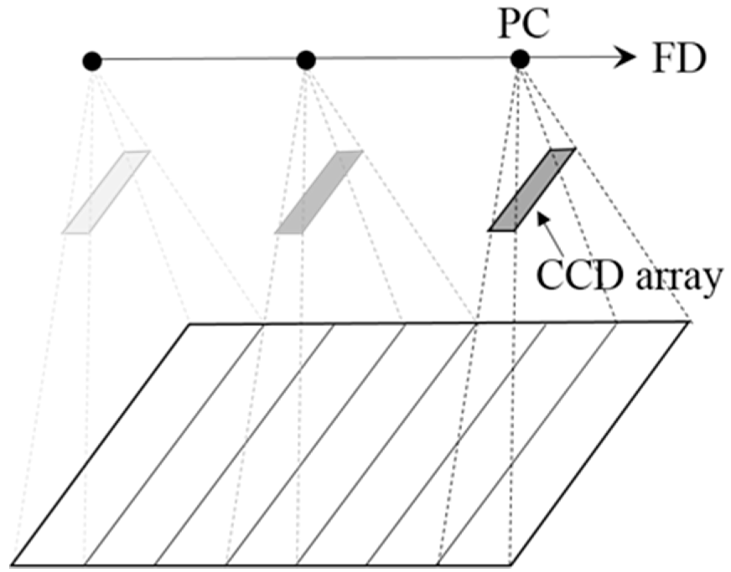
Figure 2.
Comparison of imaging geometry of the along- and the across-track components of pushbroom imagery: (a) geometry of the along-track component; and (b) geometry of the across-track component.
Figure 2.
Comparison of imaging geometry of the along- and the across-track components of pushbroom imagery: (a) geometry of the along-track component; and (b) geometry of the across-track component.
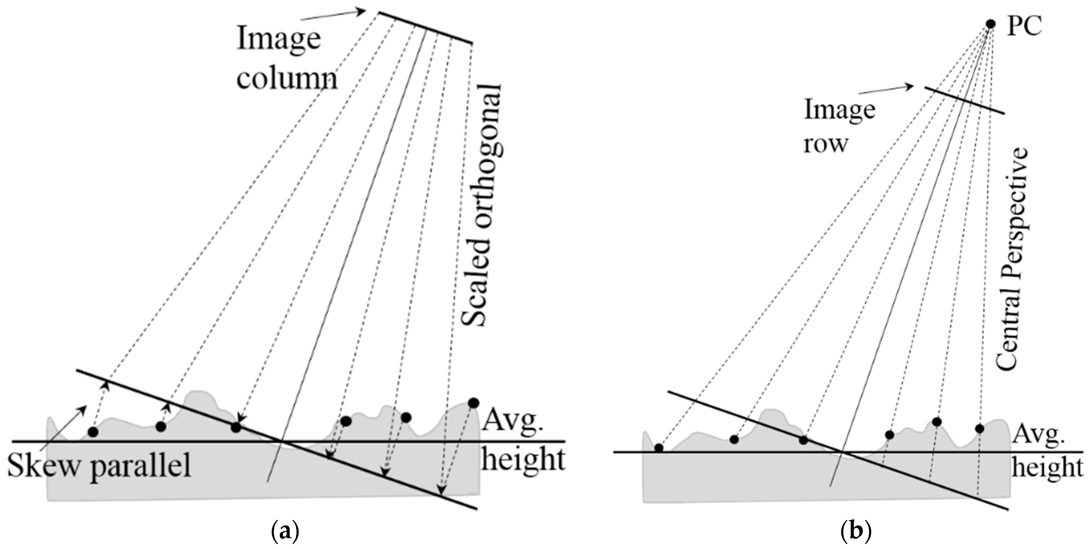
Figure 3.
The search space of the first step search.
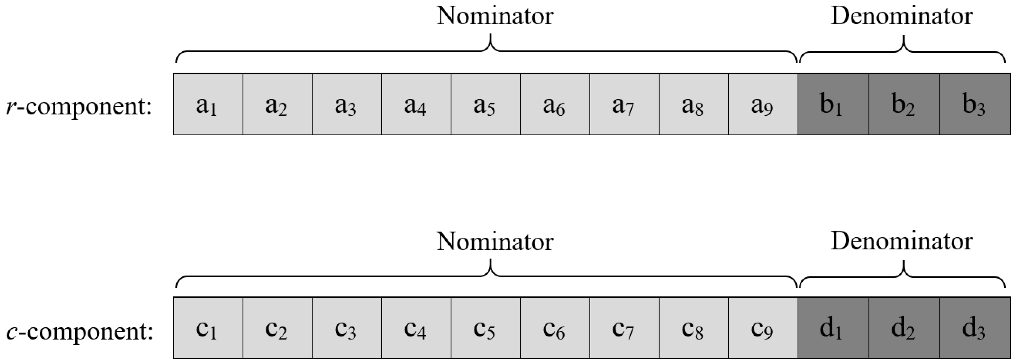
Figure 4.
Search space of the second step search.
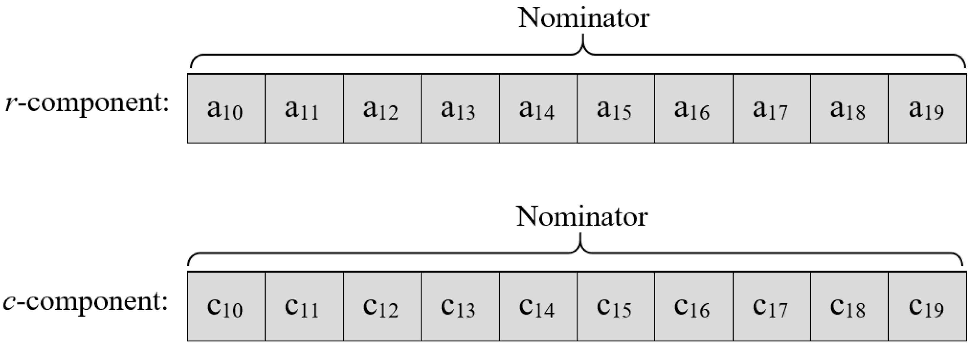
Figure 5.
Flowchart of the proposed method.

Figure 6.
Scatter plot of residual errors of the proposed method (using only six GCPs): (a) Isfahan dataset, SPOT-1A; (b) Isfahan dataset, SPOT-1B; (c) Hamedan dataset, IKONOS-Geo; and (d) Uromieh dataset, GeoEye-Geo.
Figure 6.
Scatter plot of residual errors of the proposed method (using only six GCPs): (a) Isfahan dataset, SPOT-1A; (b) Isfahan dataset, SPOT-1B; (c) Hamedan dataset, IKONOS-Geo; and (d) Uromieh dataset, GeoEye-Geo.

Figure 7.
Graphical comparison of accuracies obtained from the proposed method and GA-optimized RFMs: (a) Isfahan dataset, SPOT-1A; (b) Isfahan dataset, SPOT-1B; (c) Hamedan dataset, IKONOS-Geo; and (d) Uromieh dataset, GeoEye-Geo.
Figure 7.
Graphical comparison of accuracies obtained from the proposed method and GA-optimized RFMs: (a) Isfahan dataset, SPOT-1A; (b) Isfahan dataset, SPOT-1B; (c) Hamedan dataset, IKONOS-Geo; and (d) Uromieh dataset, GeoEye-Geo.

Figure 8.
Graphical comparison of accuracies obtained from the proposed method and conventional RFMs: (a) Isfahan dataset, SPOT-1A; (b) Isfahan dataset, SPOT-1B; (c) Hamedan dataset, IKONOS-Geo; and (d) Uromieh dataset, GeoEye-Geo.
Figure 8.
Graphical comparison of accuracies obtained from the proposed method and conventional RFMs: (a) Isfahan dataset, SPOT-1A; (b) Isfahan dataset, SPOT-1B; (c) Hamedan dataset, IKONOS-Geo; and (d) Uromieh dataset, GeoEye-Geo.


Table 1.
Specifications of the dataset used.
| Dataset | Isfahan | Hamedan | Uromieh | |
|---|---|---|---|---|
| Platform | SPOT-3 | SPOT-3 | IKONOS-2 | GeoEye-1 |
| Sensor | HRV | HRV | Panchromatic | Panchromatic |
| Product | Level 1A | Level 1B | Geo | Geo |
| Acquisition | July 1993 | July 1993 | October 2000 | August 2010 |
| Off-nadir angle | 19.01°W | 19.01°W | 20.4°E | 0.84°W |
| Pixel Size | 13 μ | 13 μ | 12 μ | 8 μ |
| GSD | 10 m | 10 m | 0.82 m | 0.41 m |
| Sampling Rate | 665 line/s | 665 line/s | 6500 line/s | 10,000 line/s |
| No. of GCPs | 28 | 28 | 30 | 50 |
| Terrain relief | 613.10 m | 613.10 m | 121.60 m | 185.00 m |
| Average terrain altitude | 1493.20 m | 1493.20 m | 1798.60 m | 1369.70 m |
Table 2.
Results obtained from the proposed method using different number of GCPs over Isfahan dataset, SPOT-1A.
Table 2.
Results obtained from the proposed method using different number of GCPs over Isfahan dataset, SPOT-1A.
| GCP, CP | 1st Step Search | 2nd Step Search | ||||||||||||||||||
|---|---|---|---|---|---|---|---|---|---|---|---|---|---|---|---|---|---|---|---|---|
| δr (Pixel) | δc (Pixel) | rmse (Pixel) | cond. | P1,P2,P3,P4 | df | δr (Pixel) | δc (Pixel) | rmse (Pixel) | cond. | P1,P2,P3,P4 | df | |||||||||
| Mean | std. | max. | Mean | std. | max. | Mean | std. | max. | Mean | std. | max. | |||||||||
| 4, 24 | −0.04 | 0.52 | 1.16 | 2.97 | 7.93 | 23.1 | 8.33 | 0.7 × 101 | 4,0,3,1 | 0 | ||||||||||
| 5, 23 | 0.01 | 0.49 | 1.12 | 4.50 | 5.53 | 11.6 | 7.06 | 2.6 × 101 | 3,1,5,0 | 1 | ||||||||||
| 6, 22 | −0.01 | 0.50 | 1.02 | 0.32 | 0.51 | 1.56 | 0.77 | 4.7 × 10⁴ | 4,1,4,2 | 1 | ||||||||||
| 8, 20 | −0.02 | 0.45 | −0.85 | 0.05 | 0.52 | 1.43 | 0.83 | 1.7 × 10² | 6,2,6,0 | 2 | ||||||||||
| 10, 18 | −0.02 | 0.39 | −0.79 | −0.01 | 0.46 | −1.22 | 0.60 | 0.8 × 101 | 4,0,4,2 | 10 | −0.04 | 0.38 | −0.71 | 0.01 | 0.36 | 0.61 | 0.52 | 2.3 × 101 | 5,0,5,2 | 8 |
| 12, 16 | −0.02 | 0.33 | −0.80 | 0.01 | 0.49 | −1.24 | 0.62 | 6.5 × 10⁴ | 5,0,4,2 | 13 | −0.09 | 0.34 | −0.60 | 0.06 | 0.39 | −0.86 | 0.54 | 1.9 × 10² | 7,0,8,2 | 7 |
| 14, 14 | −0.01 | 0.40 | −0.71 | 0.03 | 0.37 | 0.71 | 0.56 | 2.1 × 10⁴ | 6,1,9,1 | 11 | −0.02 | 0.35 | −0.64 | 0.06 | 0.39 | 0.75 | 0.52 | 9.3 × 10⁴ | 8,1,10,1 | 8 |
| 16, 12 | −0.02 | 0.32 | −0.64 | 0.02 | 0.27 | 0.66 | 0.51 | 7.7 × 10² | 7,1,7,2 | 15 | −0.03 | 0.32 | 0.66 | 0.03 | 0.28 | −0.61 | 0.45 | 7.9 × 10³ | 13,1,12,2 | 5 |
| 18, 10 | −0.01 | 0.34 | −0.59 | 0.02 | 0.27 | 0.65 | 0.50 | 2.4 × 101 | 4,1,7,2 | 22 | −0.03 | 0.29 | −0.52 | 0.02 | 0.29 | 0.65 | 0.44 | 1.7 × 10² | 9,1,10,2 | 14 |
| 20, 8 | −0.00 | 0.33 | −0.58 | 0.02 | 0.22 | 0.59 | 0.44 | 7.0 × 10² | 7,2,7,1 | 23 | −0.07 | 0.26 | −0.48 | 0.02 | 0.17 | 0.53 | 0.35 | 6.2 × 10³ | 11,2,9,1 | 17 |
Table 3.
Results obtained from the proposed method using different number of GCPs over Isfahan dataset, SPOT-1B.
Table 3.
Results obtained from the proposed method using different number of GCPs over Isfahan dataset, SPOT-1B.
| GCP, CP | 1st Step Search | 2nd Step Search | ||||||||||||||||||
|---|---|---|---|---|---|---|---|---|---|---|---|---|---|---|---|---|---|---|---|---|
| δr (Pixel) | δc (Pixel) | rmse (Pixel) | cond. | P1,P2,P3,P4 | df | δr (Pixel) | δc (Pixel) | rmse (Pixel) | cond. | P1,P2,P3,P4 | df | |||||||||
| Mean | std. | max. | Mean | std. | max. | Mean | std. | max. | Mean | std. | max. | |||||||||
| 4, 24 | 0.13 | 0.62 | 1.74 | −0.50 | 0.67 | −2.36 | 1.04 | 1.7 × 101 | 3,1,4,0 | 0 | ||||||||||
| 5, 23 | 0.08 | 0.54 | 1.15 | 0.01 | 0.64 | −1.36 | 0.85 | 2.7 × 101 | 3,1,4,1 | 1 | ||||||||||
| 6, 22 | 0.06 | 0.57 | 1.50 | −0.04 | 0.61 | −1.39 | 0.82 | 5.7 × 101 | 4,1,4,1 | 2 | ||||||||||
| 8, 20 | 0.03 | 0.49 | 1.09 | −0.00 | 0.51 | −1.57 | 0.75 | 1.4 × 101 | 3,1,4,2 | 6 | −0.02 | 0.35 | 1.10 | 0.01 | 0.50 | 1.20 | 0.71 | 6.7 × 101 | 4,1,6,2 | 3 |
| 10, 18 | −0.04 | 0.52 | 1.09 | −0.02 | 0.53 | −1.25 | 0.69 | 2.3 × 10² | 4,1,6,1 | 8 | 0.00 | 0.54 | 1.21 | −0.01 | 0.43 | −1.26 | 0.68 | 8.9 × 101 | 5,1,9,1 | 4 |
| 12, 16 | −0.09 | 0.48 | 1.19 | −0.02 | 0.42 | −1.40 | 0.69 | 5.7 × 101 | 4,1,5,1 | 13 | −0.01 | 0.49 | 1.13 | −0.01 | 0.28 | −0.74 | 0.59 | 8.5 × 101 | 5,1,7,1 | 10 |
| 14, 14 | −0.07 | 0.50 | 1.04 | −0.03 | 0.40 | −1.31 | 0.68 | 3.9 × 101 | 4,0,6,1 | 17 | −0.02 | 0.50 | 1.04 | −0.02 | 0.32 | −0.91 | 0.62 | 7.9 × 101 | 5,0,9,1 | 13 |
| 16, 12 | 0.03 | 0.49 | 1.18 | −0.02 | 0.45 | −0.88 | 0.68 | 0.6 × 101 | 4,0,9,3 | 16 | −0.02 | 0.45 | 0.93 | −0.01 | 0.50 | −0.94 | 0.61 | 4.3 × 10² | 9,0,13,3 | 7 |
| 18, 10 | 0.00 | 0.52 | −1.18 | −0.03 | 0.22 | −0.56 | 0.57 | 2.9 × 101 | 6,0,6,3 | 21 | −0.01 | 0.50 | −1.09 | 0.01 | 0.17 | −0.31 | 0.59 | 3.4 × 101 | 11,0,7,3 | 15 |
| 20, 8 | −0.01 | 0.53 | 0.99 | −0.01 | 0.23 | −0.53 | 0.54 | 7.6 × 10³ | 8,1,6,3 | 22 | −0.02 | 0.59 | 0.94 | −0.00 | 0.19 | −0.29 | 0.50 | 7.7 × 10⁴ | 9,1,7,3 | 20 |
Table 4.
Results obtained from the proposed method using different number of GCPs over Hamedan dataset, IKONOS-2.
Table 4.
Results obtained from the proposed method using different number of GCPs over Hamedan dataset, IKONOS-2.
| GCP, CP | 1st Step Search | 2nd Step Search | ||||||||||||||||||
|---|---|---|---|---|---|---|---|---|---|---|---|---|---|---|---|---|---|---|---|---|
| δr (Pixel) | δc (Pixel) | rmse (Pixel) | cond. | P1,P2,P3,P4 | df | δr (Pixel) | δc (Pixel) | rmse (Pixel) | cond. | P1,P2,P3,P4 | df | |||||||||
| Mean | std. | max. | Mean | std. | max. | Mean | std. | max. | Mean | std. | max. | |||||||||
| 4, 26 | 0.27 | 0.78 | 1.68 | 0.18 | 0.60 | 1.87 | 1.09 | 0.3 × 101 | 3,1,3,0 | 1 | ||||||||||
| 5, 25 | −0.09 | 0.49 | −1.01 | 0.10 | 0.61 | 1.96 | 0.84 | 8.4 × 10² | 4,0,4,1 | 1 | ||||||||||
| 6, 24 | −0.07 | 0.38 | 0.83 | 0.09 | 0.49 | 1.38 | 0.77 | 1.5 × 10³ | 4,1,4,2 | 1 | ||||||||||
| 8, 22 | −0.08 | 0.37 | −0.89 | 0.06 | 0.39 | 0.74 | 0.61 | 1.1 × 10⁵ | 5,1,5,1 | 4 | ||||||||||
| 10, 20 | −0.05 | 0.34 | −0.81 | 0.06 | 0.38 | 0.79 | 0.53 | 8.3 × 10⁴ | 5,1,7,2 | 5 | −0.03 | 0.34 | −0.81 | 0.03 | 0.38 | −0.81 | 0.53 | 8.3 × 10⁴ | 5,1,7,2 | 5 |
| 12, 18 | −0.04 | 0.37 | −0.67 | 0.05 | 0.37 | 0.77 | 0.52 | 6.7 × 10⁵ | 6,2,7,2 | 7 | −0.04 | 0.37 | −0.99 | 0.02 | 0.35 | −0.99 | 0.51 | 2.1 × 10⁶ | 10,2,8,2 | 2 |
| 14, 16 | −0.03 | 0.26 | −0.55 | −0.05 | 0.35 | −0.67 | 0.45 | 6.3 × 10⁵ | 7,1,7,2 | 11 | −0.02 | 0.28 | −0.55 | 0.04 | 0.40 | −0.55 | 0.45 | 6.3 × 10⁵ | 7,1,7,2 | 11 |
| 16, 14 | −0.05 | 0.27 | −0.57 | −0.06 | 0.35 | −0.71 | 0.44 | 2.5 × 10⁶ | 8,2,6,3 | 13 | −0.03 | 0.26 | −0.55 | −0.05 | 0.33 | −0.55 | 0.42 | 1.4 × 10⁶ | 9,2,8,3 | 10 |
| 18, 12 | −0.04 | 0.29 | −0.61 | −0.03 | 0.30 | −0.48 | 0.42 | 2.7 × 10⁶ | 9,2,6,3 | 16 | −0.00 | 0.19 | −0.35 | 0.00 | 0.34 | −0.35 | 0.40 | 1.5 × 10⁶ | 11,2,9,3 | 11 |
| 20, 10 | −0.03 | 0.22 | −0.31 | −0.02 | 0.31 | −0.62 | 0.42 | 7.2 × 10⁵ | 7,1,5,2 | 25 | −0.01 | 0.17 | −0.42 | −0.01 | 0.31 | −0.42 | 0.38 | 4.3 × 10⁴ | 12,1,6,2 | 19 |
Table 5.
Results obtained from the proposed method using different number of GCPs over Uromieh dataset, GeoEye-1.
Table 5.
Results obtained from the proposed method using different number of GCPs over Uromieh dataset, GeoEye-1.
| GCP, CP | 1st Step Search | 2nd Step Search | ||||||||||||||||||
|---|---|---|---|---|---|---|---|---|---|---|---|---|---|---|---|---|---|---|---|---|
| δr (Pixel) | δc (Pixel) | rmse (Pixel) | cond. | P1,P2,P3,P4 | df | δr (Pixel) | δc (Pixel) | rmse (Pixel) | cond. | P1,P2,P3,P4 | df | |||||||||
| Mean | std. | max. | Mean | std. | max. | Mean | std. | max. | Mean | std. | max. | |||||||||
| 4, 46 | −0.04 | 0.48 | 0.94 | 0.07 | 0.61 | 1.18 | 0.69 | 0.2 × 101 | 3,0,3,1 | 1 | ||||||||||
| 5, 45 | 0.02 | 0.47 | 0.93 | −0.02 | 0.55 | 1.02 | 0.63 | 1.0 × 101 | 4,0,3,1 | 2 | ||||||||||
| 6, 44 | −0.00 | 0.48 | 0.95 | 0.05 | 0.53 | 1.01 | 0.60 | 1.1 × 101 | 4,0,4,1 | 3 | ||||||||||
| 8, 42 | −0.05 | 0.48 | 0.92 | 0.05 | 0.54 | −0.95 | 0.61 | 2.2 × 101 | 5,0,6,0 | 5 | −0.03 | 0.43 | 0.92 | 0.04 | 0.50 | −0.95 | 0.61 | 2.2 × 101 | 5,0,6,0 | 5 |
| 10, 40 | −0.04 | 0.49 | −0.82 | 0.04 | 0.51 | 0.88 | 0.60 | 1.6 × 10⁵ | 6,2,4,2 | 6 | −0.02 | 0.43 | −0.85 | 0.04 | 0.48 | 0.86 | 0.58 | 1.6 × 10⁵ | 6,2,4,2 | 6 |
| 12, 38 | −0.03 | 0.49 | 1.10 | −0.00 | 0.46 | −0.91 | 0.59 | 9.1 × 10⁶ | 5,2,6,1 | 10 | 0.03 | 0.46 | 1.10 | −0.04 | 0.43 | −0.91 | 0.59 | 9.1 × 10⁶ | 5,2,6,1 | 10 |
| 14, 36 | −0.06 | 0.50 | 0.94 | −0.02 | 0.36 | 0.77 | 0.58 | 1.4 × 10⁶ | 5,2,6,1 | 14 | −0.01 | 0.46 | 0.92 | −0.02 | 0.37 | −0.88 | 0.57 | 1.6 × 10⁶ | 6,2,9,1 | 10 |
| 16, 34 | 0.01 | 0.46 | −0.84 | −0.04 | 0.39 | 0.92 | 0.58 | 1.7 × 10⁶ | 5,2,6,1 | 18 | −0.01 | 0.41 | −0.86 | −0.03 | 0.37 | 0.78 | 0.56 | 1.4 × 10⁶ | 6,2,7,1 | 16 |
| 18, 32 | −0.03 | 0.47 | −0.86 | −0.03 | 0.33 | 0.78 | 0.56 | 1.5 × 10² | 5,1,5,0 | 25 | −0.02 | 0.42 | −0.87 | −0.03 | 0.34 | −0.75 | 0.55 | 2.1 × 10⁵ | 10,1,8,0 | 17 |
| 20, 30 | −0.01 | 0.48 | 0.92 | −0.03 | 0.36 | 0.76 | 0.54 | 1.6 × 10² | 5,1,5,0 | 29 | −0.01 | 0.45 | 0.92 | −0.04 | 0.37 | 0.76 | 0.54 | 2.2 × 10⁴ | 6,1,10,0 | 23 |
Table 6.
Results obtained from GA-optimized and convention RFMs using different number of GCPs over Isfahan dataset, SPOT-1A.
Table 6.
Results obtained from GA-optimized and convention RFMs using different number of GCPs over Isfahan dataset, SPOT-1A.
| GCP, CP | GA-Optimized RFM (10 Times Run) | Conventional RFM | |||||||||||||||||||
|---|---|---|---|---|---|---|---|---|---|---|---|---|---|---|---|---|---|---|---|---|---|
| δr (Pixel) | δc (Pixel) | rmse (Pixel) | cond. | Iterations | P1,P2,P3,P4 | df | δr (Pixel) | δc (Pixel) | rmse (Pixel) | cond. | P1,P2,P3,P4 | df | |||||||||
| Mean | std. | max. | Mean | std. | max. | Mean | std. | max. | Mean | std. | max. | ||||||||||
| 8, 20 | 0.03 | 0.57 | −1.38 | −0.07 | 0.61 | −1.40 | 0.91 | 2.1 × 101 | 379 | 6,2,4,2 | 2 | −0.32 | 1.16 | −2.65 | 1.28 | 1.84 | 6.91 | 2.56 | 3.4 × 10² | 4,3,4,3 | 2 |
| 10, 18 | 0.02 | 0.51 | 1.18 | 0.05 | 0.59 | −1.22 | 0.88 | 4.5 × 10² | 280 | 5,4,6,2 | 3 | −0.17 | 1.14 | −2.49 | 0.19 | 0.95 | −2.79 | 1.51 | 1.3 × 10² | 5,4,5,4 | 2 |
| 12, 16 | 0.03 | 0.49 | 1.08 | −0.05 | 0.59 | 1.12 | 0.87 | 4.1 × 10³ | 367 | 6,3,10,2 | 3 | 0.24 | 0.57 | −1.12 | 0.63 | 0.63 | 1.54 | 1.10 | 2.9 × 10² | 6,5,6,5 | 2 |
| 14, 14 | 0.02 | 0.45 | −1.03 | −0.05 | 0.52 | 1.52 | 0.83 | 2.2 × 10³ | 144 | 9,5,8,2 | 4 | −0.15 | 0.82 | −1.74 | 0.59 | 0.83 | 1.93 | 1.33 | 7.5 × 10⁵ | 7,6,7,6 | 2 |
| 16, 12 | −0.01 | 0.50 | 1.10 | −0.03 | 0.51 | 0.87 | 0.79 | 5.4 × 10³ | 195 | 9,4,7,4 | 8 | 0.16 | 0.83 | −2.10 | −0.14 | 0.87 | 2.05 | 1.23 | 2.5 × 10⁵ | 8,7,8,7 | 2 |
| 18, 10 | 0.02 | 0.49 | −0.87 | −0.00 | 0.48 | 1.10 | 0.73 | 3.7 × 10⁴ | 96 | 11,4,9,4 | 8 | 0.24 | 0.74 | −1.49 | −0.31 | 0.95 | −2.28 | 1.28 | 3.6 × 10⁵ | 9,8,9,8 | 2 |
| 20, 8 | 0.01 | 0.52 | 1.14 | −0.01 | 0.47 | −0.72 | 0.71 | 7.2 × 10⁴ | 115 | 12,9,10,7 | 3 | 0.08 | 1.76 | −3.85 | 0.44 | 0.77 | 1.43 | 1.98 | 5.1 × 10⁵ | 10,9,10,9 | 2 |
Table 7.
Results obtained from GA-optimized and convention RFMs using different number of GCPs over Isfahan dataset, SPOT-1B.
Table 7.
Results obtained from GA-optimized and convention RFMs using different number of GCPs over Isfahan dataset, SPOT-1B.
| GCP, CP | GA-Optimized RFM (10 Times Run) | Conventional RFM | |||||||||||||||||||
|---|---|---|---|---|---|---|---|---|---|---|---|---|---|---|---|---|---|---|---|---|---|
| δr (Pixel) | δc (Pixel) | rmse (Pixel) | cond. | Iterations | P1,P2,P3,P4 | df | δr (Pixel) | δc (Pixel) | rmse (Pixel) | cond. | P1,P2,P3,P4 | df | |||||||||
| Mean | std. | max. | Mean | std. | max. | Mean | std. | max. | Mean | std. | max. | ||||||||||
| 8, 20 | 0.15 | 0.65 | 1.20 | 0.33 | 0.71 | −2.03 | 1.01 | 8.1 × 101 | 500 | 5,2,5,2 | 2 | −0.75 | 1.74 | −4.87 | −0.58 | 1.44 | −4.76 | 2.46 | 2.5 × 101 | 4,3,4,3 | 2 |
| 10, 18 | −0.09 | 0.57 | 1.48 | 0.04 | 0.70 | −1.84 | 0.92 | 3.2 × 10² | 374 | 5,2,5,2 | 6 | −0.11 | 1.07 | −1.89 | −0.08 | 0.62 | −1.26 | 1.24 | 1.6 × 10² | 5,4,5,4 | 2 |
| 12, 16 | −0.08 | 0.57 | 1.40 | 0.05 | 0.69 | −1.60 | 0.92 | 8.1 × 101 | 380 | 6,3,6,4 | 5 | 0.12 | 0.83 | 1.72 | −0.70 | 0.83 | −2.44 | 1.38 | 3.3 × 10² | 6,5,6,5 | 2 |
| 14, 14 | −0.05 | 0.55 | −1.16 | 0.06 | 0.63 | −1.23 | 0.87 | 4.3 × 10² | 402 | 6,4,5,2 | 11 | −0.16 | 0.90 | 1.84 | −0.34 | 1.31 | −3.16 | 1.64 | 2.2 × 10⁴ | 7,6,7,6 | 2 |
| 16, 12 | −0.09 | 0.60 | 1.79 | 0.05 | 0.68 | −1.47 | 0.94 | 5.1 × 10² | 248 | 9,5,7,4 | 7 | −0.12 | 0.87 | −1.84 | −0.62 | 0.91 | −2.05 | 1.43 | 5.8 × 10⁴ | 8,7,8,7 | 2 |
| 18, 10 | 0.07 | 0.41 | 1.14 | 0.06 | 0.49 | 0.91 | 0.77 | 6.7 × 10² | 418 | 9,6,7,7 | 7 | 0.19 | 0.84 | 1.60 | 0.02 | 0.71 | −1.22 | 1.12 | 4.6 × 10⁵ | 9,8,9,8 | 2 |
| 20, 8 | −0.03 | 0.47 | 0.77 | 0.04 | 0.39 | −0.55 | 0.55 | 5.9 × 10³ | 311 | 11,4,9,8 | 8 | −0.12 | 1.27 | 1.72 | 0.92 | 3.90 | 1.68 | 4.22 | 7.1 × 10⁵ | 10,9,10,9 | 2 |
Table 8.
Results obtained from GA-optimized and convention RFMs using different number of GCPs over Hamedan dataset, IKONOS-2.
Table 8.
Results obtained from GA-optimized and convention RFMs using different number of GCPs over Hamedan dataset, IKONOS-2.
| GCP, CP | GA-optimized RFM (10 Times Run) | Conventional RFM | |||||||||||||||||||
|---|---|---|---|---|---|---|---|---|---|---|---|---|---|---|---|---|---|---|---|---|---|
| δr (Pixel) | δc (Pixel) | rmse (Pixel) | cond. | Iterations | P1,P2,P3,P4 | df | δr (Pixel) | δc (Pixel) | rmse (Pixel) | cond. | P1,P2,P3,P4 | df | |||||||||
| Mean | std. | max. | Mean | std. | max. | Mean | std. | max. | Mean | std. | max. | ||||||||||
| 8, 22 | 0.08 | 0.39 | −0.91 | 0.07 | 0.48 | −1.19 | 0.74 | 1.7 × 10⁵ | 500 | 6,2,5,2 | 1 | 0.07 | 0.69 | −1.39 | −0.48 | 0.64 | −1.64 | 1.07 | 7.6 × 101 | 4,3,4,3 | 2 |
| 10, 20 | −0.08 | 0.37 | 0.93 | 0.08 | 0.41 | −1.22 | 0.62 | 2.4 × 10⁵ | 349 | 7,1,3,2 | 7 | −0.09 | 0.52 | −1.07 | −0.41 | 0.64 | −1.61 | 0.93 | 4.8 × 10³ | 5,4,5,4 | 2 |
| 12, 18 | −0.07 | 0.38 | −0.89 | 0.06 | 0.39 | −1.00 | 0.61 | 1.3 × 10⁶ | 271 | 4,4,4,3 | 9 | 0.17 | 0.44 | −1.01 | −0.29 | 0.54 | 1.30 | 0.78 | 9.2 × 10⁵ | 6,5,6,5 | 2 |
| 14, 16 | −0.08 | 0.39 | −0.51 | −0.05 | 0.38 | −1.05 | 0.59 | 7.1 × 10⁴ | 326 | 6,4,8,3 | 7 | −0.33 | 1.03 | −1.97 | 0.01 | 0.71 | 1.86 | 1.30 | 2.5 × 10⁵ | 7,6,7,6 | 2 |
| 16, 14 | −0.05 | 0.33 | 0.39 | 0.06 | 0.39 | −0.90 | 0.54 | 4.2 × 10⁶ | 450 | 9,6,7,7 | 3 | 0.02 | 0.51 | 1.09 | 0.27 | 0.98 | 2.39 | 1.13 | 6.3 × 10⁵ | 8,7,8,7 | 2 |
| 18, 12 | −0.00 | 0.38 | 0.64 | 0.02 | 0.36 | −0.87 | 0.52 | 4.4 × 10⁵ | 300 | 4,8,9,7 | 8 | 0.40 | 0.89 | 2.20 | −0.05 | 0.76 | 1.33 | 1.24 | 3.1 × 10⁶ | 9,8,9,8 | 2 |
| 20, 10 | −0.03 | 0.31 | −0.48 | −0.02 | 0.32 | −0.99 | 0.49 | 3.8 × 10⁵ | 264 | 7,8,9,11 | 5 | 0.65 | 2.97 | 8.87 | −0.45 | 2.39 | −4.09 | 3.95 | 5.8 × 10⁶ | 10,9,10,9 | 2 |
Table 9.
Results obtained from GA-optimized and convention RFMs using different number of GCPs over Uromieh dataset, GeoEye-1.
Table 9.
Results obtained from GA-optimized and convention RFMs using different number of GCPs over Uromieh dataset, GeoEye-1.
| GCP, CP | GA-Optimized RFM (10 Times Run) | Conventional RFM | |||||||||||||||||||
|---|---|---|---|---|---|---|---|---|---|---|---|---|---|---|---|---|---|---|---|---|---|
| δr (Pixel) | δc (Pixel) | rmse (Pixel) | cond. | Iterations | P1,P2,P3,P4 | df | δr (Pixel) | δc (Pixel) | rmse (Pixel) | cond. | P1,P2,P3,P4 | df | |||||||||
| Mean | std. | max. | Mean | std. | max. | Mean | std. | max. | Mean | std. | max. | ||||||||||
| 8, 42 | −0.03 | 0.48 | −1.00 | 0.03 | 0.55 | 1.23 | 0.69 | 7.2 × 10³ | 472 | 5,2,5,2 | 2 | 0.00 | 0.87 | −1.82 | 0.00 | 0.78 | 2.02 | 1.18 | 1.0 × 10² | 4,3,4,3 | 2 |
| 10, 40 | −0.02 | 0.46 | −1.17 | 0.05 | 0.63 | 1.25 | 0.69 | 2.8 × 10⁶ | 387 | 4,3,6,3 | 4 | −0.08 | 1.07 | −3.47 | 0.02 | 0.95 | −3.34 | 1.44 | 7.4 × 10² | 5,4,5,4 | 2 |
| 12, 38 | −0.05 | 0.49 | −1.18 | 0.02 | 0.57 | 1.65 | 0.69 | 3.6 × 10⁷ | 423 | 4,5,4,4 | 7 | −0.37 | 0.76 | −2.78 | −0.14 | 1.61 | −7.14 | 1.83 | 2.6 × 10⁵ | 6,5,6,5 | 2 |
| 14, 36 | 0.02 | 0.44 | 0.87 | 0.04 | 0.53 | −1.42 | 0.66 | 9.2 × 10⁶ | 500 | 4,4,7,4 | 9 | −0.52 | 0.75 | −1.62 | −0.40 | 1.55 | −6.86 | 1.74 | 1.7 × 10⁶ | 7,6,7,6 | 2 |
| 16, 34 | −0.02 | 0.47 | −1.02 | 0.00 | 0.55 | 1.28 | 0.66 | 5.5 × 10⁶ | 500 | 6,4,7,3 | 12 | −0.03 | 1.17 | 2.80 | −0.27 | 1.62 | −6.23 | 3.64 | 2.4 × 10⁶ | 8,7,8,7 | 2 |
| 18, 32 | 0.01 | 0.48 | −1.05 | −0.04 | 0.56 | 1.08 | 0.65 | 5.1 × 10⁶ | 500 | 8,4,6,7 | 11 | 0.86 | 5.71 | −13.17 | −0.42 | 1.16 | −4.08 | 9.09 | 5.0 × 10⁶ | 9,8,9,8 | 2 |
| 20, 30 | −0.03 | 0.46 | −0.94 | 0.02 | 0.50 | −0.99 | 0.61 | 4.7 × 10⁷ | 500 | 9,5,10,5 | 11 | −1.46 | 8.06 | 14.82 | −0.63 | 1.22 | −15.37 | 11.15 | 9.6 × 10⁶ | 10,9,10,9 | 2 |
Table 10.
Results obtained from low order polynomials using different number of GCPs over Isfahan dataset, SPOT-1A.
Table 10.
Results obtained from low order polynomials using different number of GCPs over Isfahan dataset, SPOT-1A.
| GCP, CP | First-Order Polynomial | Second-Order Polynomial | ||||||||||||||||
|---|---|---|---|---|---|---|---|---|---|---|---|---|---|---|---|---|---|---|
| δr (Pixel) | δc (Pixel) | rmse (Pixel) | cond. | df | δr (Pixel) | δc (Pixel) | rmse (Pixel) | cond. | df | |||||||||
| Mean | std. | max. | Mean | std. | max. | Mean | std. | max. | Mean | std. | max. | |||||||
| 6, 22 | −0.03 | 0.07 | 0.67 | −0.05 | 2.64 | 4.41 | 3.64 | 1.6 × 101 | 4 | |||||||||
| 8, 20 | −0.04 | 0.25 | 0.57 | 0.03 | 2.89 | 2.73 | 3.50 | 1.3 × 101 | 8 | |||||||||
| 10, 18 | −0.02 | 0.37 | 0.58 | −0.04 | 3.30 | 4.86 | 3.31 | 1.4 × 101 | 12 | |||||||||
| 12, 16 | −0.03 | 0.33 | 0.57 | −0.02 | 3.46 | 4.95 | 3.48 | 2.3 × 101 | 16 | −0.02 | 0.31 | 0.54 | 0.03 | 1.52 | 2.63 | 1.61 | 2.2 × 101 | 4 |
| 14, 14 | −0.01 | 0.35 | 0.52 | −0.01 | 3.44 | 4.62 | 3.44 | 9.7 × 101 | 20 | −0.01 | 0.28 | 0.48 | 0.02 | 1.55 | 2.61 | 1.58 | 9.7 × 101 | 8 |
| 16, 12 | −0.00 | 0.41 | 0.64 | 0.03 | 3.24 | 4.68 | 3.27 | 1.4 × 10² | 24 | −0.01 | 0.27 | 0.64 | 0.04 | 1.29 | 2.55 | 1.55 | 1.4 × 10² | 12 |
| 18, 10 | −0.02 | 0.48 | 0.80 | 0.01 | 3.05 | 4.74 | 3.08 | 2.5 × 10² | 28 | 0.02 | 0.35 | 0.65 | 0.01 | 1.29 | 2.48 | 1.51 | 2.5 × 10² | 16 |
| 20, 8 | −0.00 | 0.45 | 0.78 | 0.01 | 2.94 | 4.76 | 2.98 | 3.2 × 10² | 32 | 0.02 | 0.33 | 0.63 | −0.02 | 1.27 | 2.46 | 1.52 | 3.2 × 10² | 20 |
Table 11.
Results obtained from low order polynomials using different number of GCPs over Isfahan dataset, SPOT-1B.
Table 11.
Results obtained from low order polynomials using different number of GCPs over Isfahan dataset, SPOT-1B.
| GCP, CP | First-Order Polynomial | Second-Order Polynomial | ||||||||||||||||
|---|---|---|---|---|---|---|---|---|---|---|---|---|---|---|---|---|---|---|
| δr (Pixel) | δc (Pixel) | rmse (Pixel) | cond. | df | δr (Pixel) | δc (Pixel) | rmse (Pixel) | cond. | df | |||||||||
| Mean | std. | max. | Mean | std. | max. | Mean | std. | max. | Mean | std. | max. | |||||||
| 6, 22 | −0.04 | 0.35 | 0.55 | −0.02 | 1.23 | 2.13 | 1.19 | 1.5 × 101 | 4 | |||||||||
| 8, 20 | 0.01 | 0.38 | 0.51 | −0.01 | 1.14 | 2.09 | 1.07 | 1.3 × 101 | 8 | |||||||||
| 10, 18 | −0.02 | 0.43 | 0.50 | −0.02 | 1.15 | 2.09 | 1.08 | 1.5 × 101 | 12 | |||||||||
| 12, 16 | −0.00 | 0.42 | 0.51 | −0.02 | 1.11 | 1.93 | 1.05 | 2.2 × 101 | 16 | −0.01 | 0.31 | 0.63 | −0.01 | 1.06 | 1.11 | 1.01 | 2.2 × 101 | 4 |
| 14, 14 | −0.04 | 0.49 | 1.00 | 0.01 | 1.09 | 1.94 | 1.06 | 9.7 × 101 | 20 | −0.00 | 0.28 | 0.73 | 0.02 | 1.02 | 1.08 | 0.96 | 9.7 × 101 | 8 |
| 16, 12 | 0.02 | 0.54 | 1.06 | 0.00 | 1.16 | 1.97 | 1.06 | 1.4 × 10² | 24 | −0.02 | 0.33 | 0.67 | 0.01 | 1.04 | 1.02 | 0.96 | 1.4 × 10² | 12 |
| 18, 10 | 0.01 | 0.58 | 1.06 | −0.02 | 1.04 | 1.95 | 1.02 | 2.5 × 10² | 28 | −0.01 | 0.45 | 0.82 | 0.01 | 0.95 | 1.00 | 0.91 | 2.5 × 10² | 16 |
| 20, 8 | −0.01 | 0.56 | 1.04 | 0.01 | 1.09 | 1.94 | 1.05 | 3.2 × 10² | 32 | 0.00 | 0.45 | 0.79 | 0.01 | 0.96 | 0.98 | 0.90 | 3.2 × 10² | 20 |
Table 12.
Results obtained from low order polynomials using different number of GCPs over Hamedan dataset, IKONOS-2.
Table 12.
Results obtained from low order polynomials using different number of GCPs over Hamedan dataset, IKONOS-2.
| GCP, CP | First-Order Polynomial | Second-Order Polynomial | ||||||||||||||||
|---|---|---|---|---|---|---|---|---|---|---|---|---|---|---|---|---|---|---|
| δr (Pixel) | δc (Pixel) | rmse (Pixel) | cond. | df | δr (Pixel) | δc (Pixel) | rmse (Pixel) | cond. | df | |||||||||
| Mean | std. | max. | Mean | std. | max. | Mean | std. | max. | Mean | std. | max. | |||||||
| 6, 24 | 0.03 | 0.25 | 0.27 | 0.01 | 0.65 | 0.97 | 0.65 | 0.7 × 101 | 4 | |||||||||
| 8, 22 | 0.03 | 0.22 | 0.25 | −0.02 | 0.58 | 1.08 | 0.63 | 1.2 × 101 | 8 | |||||||||
| 10, 20 | 0.01 | 0.24 | 0.42 | −0.03 | 0.52 | 1.00 | 0.59 | 1.7 × 101 | 12 | |||||||||
| 12, 18 | 0.02 | 0.32 | 0.43 | −0.01 | 0.61 | 1.00 | 0.60 | 3.1 × 101 | 16 | 0.01 | 0.28 | 0.39 | −0.01 | 0.54 | 0.73 | 0.53 | 3.1 × 101 | 4 |
| 14, 16 | 0.00 | 0.35 | 0.45 | −0.02 | 0.57 | 0.98 | 0.58 | 8.5 × 101 | 20 | −0.00 | 0.25 | 0.58 | −0.01 | 0.48 | 0.63 | 0.51 | 8.5 × 101 | 8 |
| 16, 14 | 0.01 | 0.36 | 0.53 | −0.00 | 0.56 | 0.93 | 0.58 | 1.4 × 10² | 24 | 0.02 | 0.29 | 0.43 | −0.00 | 0.50 | 0.55 | 0.49 | 1.4 × 10² | 12 |
| 18, 12 | 0.01 | 0.36 | 0.53 | −0.01 | 0.59 | 0.96 | 0.59 | 2.3 × 10² | 28 | 0.01 | 0.30 | 0.43 | 0.01 | 0.47 | 0.55 | 0.48 | 2.3 × 10² | 16 |
| 20, 10 | 0.02 | 0.35 | 0.52 | −0.00 | 0.56 | 0.87 | 0.57 | 6.2 × 10² | 32 | 0.02 | 0.29 | 0.43 | 0.01 | 0.49 | 0.68 | 0.50 | 6.2 × 10² | 20 |
Table 13.
Results obtained from low order polynomials using different number of GCPs over Uromieh dataset, GeoEye-1.
Table 13.
Results obtained from low order polynomials using different number of GCPs over Uromieh dataset, GeoEye-1.
| GCP, CP | First-Order Polynomial | Second-Order Polynomial | ||||||||||||||||
|---|---|---|---|---|---|---|---|---|---|---|---|---|---|---|---|---|---|---|
| δr (Pixel) | δc (Pixel) | rmse (Pixel) | cond. | df | δr (Pixel) | δc (Pixel) | rmse (Pixel) | cond. | df | |||||||||
| Mean | std. | max. | Mean | std. | max. | Mean | std. | max. | Mean | std. | max. | |||||||
| 6, 44 | 0.03 | 0.31 | 0.39 | 0.06 | 0.91 | 1.59 | 0.92 | 0.6 × 101 | 4 | |||||||||
| 8, 42 | −0.01 | 0.34 | 0.35 | −0.02 | 0.84 | 1.63 | 0.88 | 1.1 × 101 | 8 | |||||||||
| 10, 40 | 0.00 | 0.33 | 0.42 | 0.01 | 0.76 | 1.66 | 0.83 | 4.6 × 101 | 12 | |||||||||
| 12, 38 | 0.02 | 0.37 | 0.50 | −0.03 | 0.75 | 1.76 | 0.84 | 3.1 × 10² | 16 | −0.01 | 0.34 | 0.42 | 0.00 | 0.25 | 0.87 | 0.61 | 3.1 × 10² | 4 |
| 14, 36 | −0.02 | 0.41 | 0.57 | −0.02 | 0.76 | 1.72 | 0.86 | 5.9 × 10² | 20 | −0.02 | 0.32 | 0.56 | −0.01 | 0.24 | 0.86 | 0.59 | 5.9 × 10² | 8 |
| 16, 34 | 0.01 | 0.42 | 0.65 | 0.01 | 0.75 | 1.66 | 0.86 | 1.2 × 10³ | 24 | 0.01 | 0.23 | 0.56 | 0.00 | 0.23 | 0.79 | 0.54 | 1.2 × 10³ | 12 |
| 18, 32 | −0.03 | 0.40 | 0.61 | −0.01 | 0.71 | 1.66 | 0.81 | 7.9 × 10³ | 28 | 0.01 | 0.21 | 0.56 | −0.01 | 0.29 | 0.64 | 0.49 | 7.9 × 10³ | 16 |
| 20, 30 | 0.00 | 0.43 | 0.79 | 0.01 | 0.69 | 1.60 | 0.81 | 1.2 × 10⁴ | 32 | 0.02 | 0.31 | 0.78 | −0.01 | 0.28 | 0.68 | 0.50 | 1.2 × 10⁴ | 20 |
Table 14.
Accuracies obtained from the proposed method using eight GCPs with respect to the bias compensated RPCs provided with Uromieh dataset, GeoEye-1.
Table 14.
Accuracies obtained from the proposed method using eight GCPs with respect to the bias compensated RPCs provided with Uromieh dataset, GeoEye-1.
| δr (Pixel) | δc (Pixel) | rmse (Pixel) | ||||
|---|---|---|---|---|---|---|
| Mean | std. | max. | Mean | std. | max. | |
| −0.00 | 0.34 | 0.66 | 0.01 | 0.45 | 0.72 | 0.53 |
© 2017 by the authors. Licensee MDPI, Basel, Switzerland. This article is an open access article distributed under the terms and conditions of the Creative Commons Attribution (CC BY) license (http://creativecommons.org/licenses/by/4.0/).
Share and Cite
MDPI and ACS Style
Jannati, M.; Valadan Zoej, M.J.; Mokhtarzade, M. A Knowledge-Based Search Strategy for Optimally Structuring the Terrain Dependent Rational Function Models. Remote Sens. 2017, 9, 345. https://doi.org/10.3390/rs9040345
AMA Style
Jannati M, Valadan Zoej MJ, Mokhtarzade M. A Knowledge-Based Search Strategy for Optimally Structuring the Terrain Dependent Rational Function Models. Remote Sensing. 2017; 9(4):345. https://doi.org/10.3390/rs9040345
Chicago/Turabian StyleJannati, Mojtaba, Mohammad Javad Valadan Zoej, and Mehdi Mokhtarzade. 2017. "A Knowledge-Based Search Strategy for Optimally Structuring the Terrain Dependent Rational Function Models" Remote Sensing 9, no. 4: 345. https://doi.org/10.3390/rs9040345
Note that from the first issue of 2016, this journal uses article numbers instead of page numbers. See further details here.