
An Analysis of the Discrepancies between MODIS and INSAT-3D LSTs in High Temperatures


1
Faculty of Geography, Department of Remote Sensing and GIS, University of Tehran, Tehran, Iran
2
Center for Urban and Environmental Change, Department of Earth and Environmental Systems, Indiana State University, Terre Haute, IN 47809, USA
*
Author to whom correspondence should be addressed.
Remote Sens. 2017, 9(4), 347; https://doi.org/10.3390/rs9040347
Submission received: 17 December 2016
/
Revised: 30 March 2017
/
Accepted: 1 April 2017
/
Published: 5 April 2017
(This article belongs to the Special Issue Remote Sensing of Human-Environment Interactions along the Urban-Rural Gradient)
Abstract
:In many disciplines, knowledge on the accuracy of Land Surface Temperature (LST) as an input is of great importance. One of the most efficient methods in LST evaluation is cross validation. Well-documented and validated polar satellites with a high spatial resolution can be used as references for validating geostationary LST products. This study attempted to investigate the discrepancies between a Moderate Resolution Imaging Spectro-radiometer (MODIS) and Indian National Satellite (INSAT-3D) LSTs for high temperatures, focusing on six deserts with sand dune land cover in the Middle East from 3 March 2015 to 24 August 2016. Firstly, the variability of LSTs in the deserts of the study area was analyzed by comparing the mean, Standard Deviation (STD), skewness, minimum, and maximum criteria for each observation time. The mean value of the LST observations indicated that the MYD-D observation times are closer to those of diurnal maximum and minimum LSTs. At all times, the LST observations exhibited a negative skewness and the STD indicated higher variability during times of MOD-D. The observed maximum LSTs from MODIS collection 6 showed higher values in comparison with the last versions of LSTs for hot spot regions around the world. After the temporal, spatial, and geometrical matching of LST products, the mean of the MODIS—INSAT LST differences was calculated for the study area. The results demonstrated that discrepancies increased with temperature up to +15.5 K. The slopes of the mean differences were relatively similar for all deserts except for An Nafud, suggesting an effect of View Zenith Angle (VZA). For modeling the discrepancies between two sensors in continuous space, the Diurnal Temperature Cycles (DTC) of both sensors were constructed and compared. The sample DTC models approved the results from discrete LST subtractions and proposed the uncertainties within MODIS DTCs. The authors proposed that the observed LST discrepancies in high temperatures could be the result of inherent differences in LST retrieval algorithms.
1. Introduction
Land Surface Temperature (LST) is a key variable in the study of the surface energy budget and land surface modeling. LST is an indicator of long wave, sensible, and latent heat flux, and is used to study land surface processes and the lower boundary condition from local to global scales [1,2]. Thanks to the suitable spatio-temporal coverage of LST around the Earth, several studies have tried to assimilate LST in land surface modeling [3,4,5,6,7]. LST is critical for accurately retrieving important climatic variables, such as relative humidity [8], soil moisture [9,10], canopy evapotranspiration [11], and surface heat and water fluxes [12]. Along with using LST as an initial parameter for meteorological and climatological modeling, some studies have analyzed it as a standalone product for monitoring temperature changes, causes, and consequences. Other researchers have used it as an indicator of other parameter changes in many disciplines [13,14,15,16,17,18,19,20].
LST is a manifestation of inner and subsurface interactions under the influence of physical and chemical parameters governed by 3D-heat transfer modeling. Holmes et al. [21] introduced a method for calculating the near subsurface temperature retrieval from a single measurement. Such a method is comparable to satellite retrieved LSTs from the microwave spectrum emanating from a shallow subsurface, which for arid soils with a low level of soil moisture, is from deeper layers. LST can be retrieved either from polar or geostationary satellites. Polar-orbiting satellites provide almost a full coverage of the Earth. Since these satellites orbit at a much lower altitude than geostationary satellites (about 700 km versus 36,000 km), they provide LST data at a much higher spatial resolution (less than 1 km) than the 4–5 km resolution currently available from geostationary satellites. In fact, by focusing on sensing in the same region, a geostationary satellite is able to acquire high temporal resolution LSTs.
The accuracy of LST is a function of many factors such as cloud mask performance, compensation for the attenuation of atmosphere, change of surface emissivity with wavelength, Signal to Noise Ratio (SNR), radiometric calibration, satiability of spectral response function, and VZA. Therefore, it is necessary to validate the LST to measure the error. According to Li et al. [22], LST validation methods can be categorized into three groups: the temperature-based method, the radiance-based method, and the cross validation method. The ground validation of LST is restricted to a few homogeneous land covers. The radiance-based method does not need ground measurements but strongly depends on the accuracy of radiative transfer models, atmospheric profiles, and emissivity at a pixel scale. In cross-validation, a LST product is regarded as the reference for comparison with LSTs derived from other platforms. In this method, spatial, temporal, and geometrical matching are important issues which should be considered. Trigo et al. [23] compared the MODIS LSTs with the Spinning Enhanced Visible and Infrared Imager (SEVIRI) for cropland, tropical forest, and spare vegetation land covers. They demonstrated that SEVIRI LSTs were larger than MODIS LSTs, and that the maximum discrepancies happened during the daytime. Gao et al. [24] evaluated LSTs from SEVIRI with MODIS for different land covers in the Iberian Peninsula and a part of Maghreb. They concluded that the maximum mean 4.9 K difference observed was dependent on time, land cover, and the VZA. Qian et al. [25] analyzed the LST/LSE discrepancies between MODIS and SEVIRI over one vegetated and two bare land covers through a view angle, time, and spatial matching procedure. The results of their study showed that SEVIRI overestimated the LST by about 1 K during the night-time and 2 K during the daytime. Cho and Suh [26] evaluated the performance of LSTs derived from a Communication, Ocean, and Meteorological Satellite (COMS) and MODIS. The results showed that the mean annual absolute difference was 2.2 K for the daytime and 1.4 for the night-time. Duan and Li [27] addressed the LST differences between MODIS and SEVIRI, considering the space, time, and viewing geometry for different seasons and times of day. They concluded that there was a 2–4 K daytime and 1–2 K night-time overestimation by SEVIRI.
None of these comparisons considered LST measurements in high temperatures (In this study, high temperatures are regarded as temperatures of more than 60 °C). In recent years, LST products have been used to identify hot and cold spots on Earth. Mildrexler et al. [28] identified some of the hot spots on Earth, and the Lut Desert was identified as the hottest one by using the maximum LST measurements from 2003 to 2009. A high reflectivity, low atmospheric attenuation, almost clear sky, high potential evaporation, low vegetation cover, and low precipitation range in deserts affect the LST value. Since different satellites have specific LST measurement limits, it is necessary to validate LST products in high temperatures. A high LST variability in deserts can also reduce the performance of coefficients calculated for LST retrieval in split window algorithms. Wan [29] redefined the Generalize Split Window (GSWA) algorithm proposed by Wan and Dozier [30], to reduce large errors in desert areas due to the high variability of LSTs, emissivity error, and aerosol impact. They showed that the collection 6 LST product (refined GSWA) could provide much better results than the previous versions (collection 4 and 5). Considering MODIS LST collection 6 as a reference, it is possible to analyze the performance of geostationary satellites in high temperatures.
This research addressed the discrepancies between INSAT-3D (hereafter referred to as INSAT) and MODIS LSTs in high temperatures. The study was organized as follows: Section 2 describes the study areas and data, Section 3 explains the methodology used for an intercomparsion, and Section 4, Section 5, and Section 6 present the results, discussion, and conclusion.
2. Study Area and Datasets
2.1. Study Areas
In order to analyze the performance of INSAT in comparison to MODIS in high temperatures, the sandy parts of six deserts located in the Middle East were chosen. The selected deserts were: Rigzar (in the Lut desert) in the southeast of Iran, An Nafud in the northern part of the Arabian Peninsula, Rub al-Khali in the south of the Arabian Peninsula, Wahiba in the west of Oman, Registan in the south of Afghanistan, and Kharan in the southwest of Pakistan. All of the selected regions are homogeneous sand dune land covers with a low vegetation cover and high temperatures. The INSAT VZA for these regions varies between 37 and 57 degrees (Figure 1). Based on monthly MODIS MOD11C3 in August 2015, the mean emissivity range of these deserts was between 0.9613–0.9579 (Figure 2).
2.2. MODIS Data
The MODIS is a sensor onboard both Terra and Aqua. MODIS has 36 bands between 0.4 and 14.4 μm. This sensor provides data with 250, 500, and 1000 m spatial resolutions. MODISs on board Terra and Aqua LST products are known as MOD11 and MYD11. For this study, MOD11A1 LST and MYD11A1 LST products were used. MOD11A1 and MOD11A1 are level three LST products at a 16 bit radiometric and 1 km spatial resolution, with tiles of daily LST products gridded in the Sinusoidal projection. A tile contains 1200 × 1200 grids in 1200 rows and 1200 columns. The exact grid size at a 1 km spatial resolution is 0.928 × 0.928 km. These products were examined under clear-sky conditions, defined in MOD35 through mapping all of the valid clear-sky LST values onto grids in the sinusoidal projection and averaging the LST values of the overlapping pixels in each grid with the overlapping areas as the weight [31]. The LST pixel values in the collection 6 daily MOD11A1 LST products were calculated in each granule by the refined GSWA [29] for bare soil, as follows:
where ∆ε and ε are the difference and the mean values of emissivity in bands 31 and 32, respectively. The emissivity values are derived according to Snyder et al. [32] from quarterly Land Cover (MOD12Q1) products. Ti and Tj are the brightness temperatures in bands 31 (10.780–11.280 µm) and 32 (11.770–12.270), respectively (Figure 3). Coefficients b0 to b7 were calculated from MODTRAN4 simulations, by considering the atmospheric boundary layer temperature, water vapor, and LST range for different VZAs (Table 1).
All of the processed MODIS LST data for this study were acquired from the U.S. Geological Survey and National Aeronautics and Space Administration (NASA) websites. LST data was comprised of 480 daily and nightly observations of Aqua and Terra, from 3 March 2015 to 24 August 2016. The MODIS sinusoidal tile grids which covered the study area were h23 v05, h21v06, h22v06, and h23v06 (Figure 1).
2.3. INSAT-3D Data
INSAT-3D is a geostationary satellite which was launched on 26 July 2013. It is equipped with IMAGER and a sounder for studying atmospheric processes every 30 min. IMAGER has six bands and the sounder has 19 bands. INSAT is located at 82° east over the equator. According to EPSA [33], LSTs are produced as follows, with a 4 km spatial resolution:
where Ti and Tj are the brightness temperatures in the Thermal Infrared 1 (TIR) and TIR2 bands, respectively (Figure 3). ε is the monthly climatology of emissivity from MODIS. The coefficients b1 to b6 were calculated from MODTRAN4 simulations; the input parameters were the temperature of the atmospheric lower boundary, the atmospheric column water vapor, the surface temperature, and the VZA (Table 1). INSAT LST products have been available since 4 March 2015 and are downloadable via www.mosdac.gov.
3. Methodology
LST comparisons of both sensors in high temperatures were conducted by the following steps: (1) Analysis of temporal variability of MOD11A1 LST products over the study area; (2) data preparation; (3) investigation of variability of LSTs in sand dune deserts; (4) spatial, angular, and temporal matching; (5) LST difference calculation for four observation times of MODIS during one day and interpolated INSAT LSTs; and (6) Comparison of LST DTCs of MODIS and INSAT. Since the LSTs for the deserts of the study area were in different scenes, all of the scenes were mosaicked together to provide a continuous field for building LST time series in each region. In the next step, data for all of study area were extracted by polygons in the study period time. These data contained the LST, time of LST observation, VZA, and QC of each pixel; to reduce the effects of clouds, only pixels flagged with a quality control (QC) value equal to zero (high quality and cloud-free ) were selected for this study.
For resampling MODIS 1 km LSTs, a mean value of 5 × 5 window and the central pixel value of 5 × 5 window were used. The comparison of the two methods showed that since the land covers (sandy regions) were homogeneous, the results were the same (For whole sections of this study, the central pixel values of MODIS LSTs were used in the resampling procedure). The local times of MODIS LST products were converted to GMT time, so that they could be compared with their corresponding pixels in INSAT. For each spatially matched LST pixel of MODIS, two time series from MODIS and INSAT were constructed. The variability of LSTs in the six deserts was investigated by histograms for whole time series, through MODIS observations. To subtract the discrete LSTs of the two sensors, angular and temporal matching was essential. In angular matching, a pixel angular alignment was conducted to assure that corresponding pixels from both sensors had similar view angles from a region. Therefore, based on Duan and Li [27], a relative difference equation was applied:
is the allowed threshold for the relative difference of the line of sight views of satellites. In this study, the recruited 0.01 threshold in [27], which is equal to a maximum change of 1% in the atmospheric path length, was used [34]. Therefore, a 5.6° VZA difference threshold was considered for the selection of corresponding pixels in both sensors. Temporal matching was performed by interpolating INSAT LST observations. Because LST observations were not available at certain points of time, a condition was defined to select only the INSAT LSTs which had at least three consecutive observations, before and after MODIS observations. Since the focus of this research was on high temperatures, MOD-D and MYD-D LST observations were subtracted from the INSAT LSTs for each pixel. In the next step, to show the LST discrepancies for all pixels, the mean LST differences for five degree intervals were calculated and plotted against the temperature for MOD-D and MYD-D. Since daily MODIS LST observations were restricted to specific times, it is not possible to analyze the trend of differences of daily MODIS LSTs and INSAT. Furthermore, due to reasons such as sensor noise, some fluctuations exist in INSAT LST observations. To interpret the behavior of the two sensors in a continuous space, the Diurnal Temperature Cycle (DTC) for pixels with high LSTs in the six study area deserts was constructed. Figure 4 shows the flowchart comparing MODIS and INSAT LSTs in high temperatures.
To estimate the DTC model parameters from LST observations, INSAT and MODIS DTCs were constructed by using the INA08 model, proposed by Inamdar et al. [35]:
with
As Figure 5 shows, ) and are the modeled LSTs for the daytime and night-time, T0 is the residual temperature around sunrise, Ta is the temperature amplitude, ω is the width over half of the period of the cosine term, tm is the time at which the temperature reaches its maximum, tsr is the time of sunrise, ts is the starting time of free attenuation, δT is the temperature difference between T0 and T(t → ∞), k is the attenuation constant, is the latitude of the location, and δ is the solar declination defined as a function of the day of year (DOY) proposed by ELAGIB et al. [36]:
For constructing the MODIS DTC model using four observations, the proposed four-parameter DTC model in [37] was applied. In this model, ts was regarded as 1 h before tss. Therefore, the number of unknown parameters (five) in the INA08 model was reduced to four parameters, which can be estimated by four MODIS observations. The DTC model has a non-linear nature, and the parameters of the model cannot be directly solved from the equations and should be obtained by fitting the model to the observations. Therefore, for finding the parameters, the Levenberg-Marquardt minimization scheme was applied to estimate the DTC model parameters by using INSAT LST observations [38].
4. Results
The overpass times of the LST products (overpass here is defined as the time at which LST is produced by overlaps) for both MYD (Aqua) and MOD (Terra) for the whole time series in the study areas of this study were: MYD daily overpass time ranged from 08:20 to 11:20 GMT; nightly MYD observations occurred between 20:40 to 23:50 GMT; daily MOD overpass time occurred from 06:00 to 08:15 GMT; and nightly MOD overpass time occurred from18:40 to 20:10 GMT.
4.1. Variability of LSTs in the Study Area Deserts
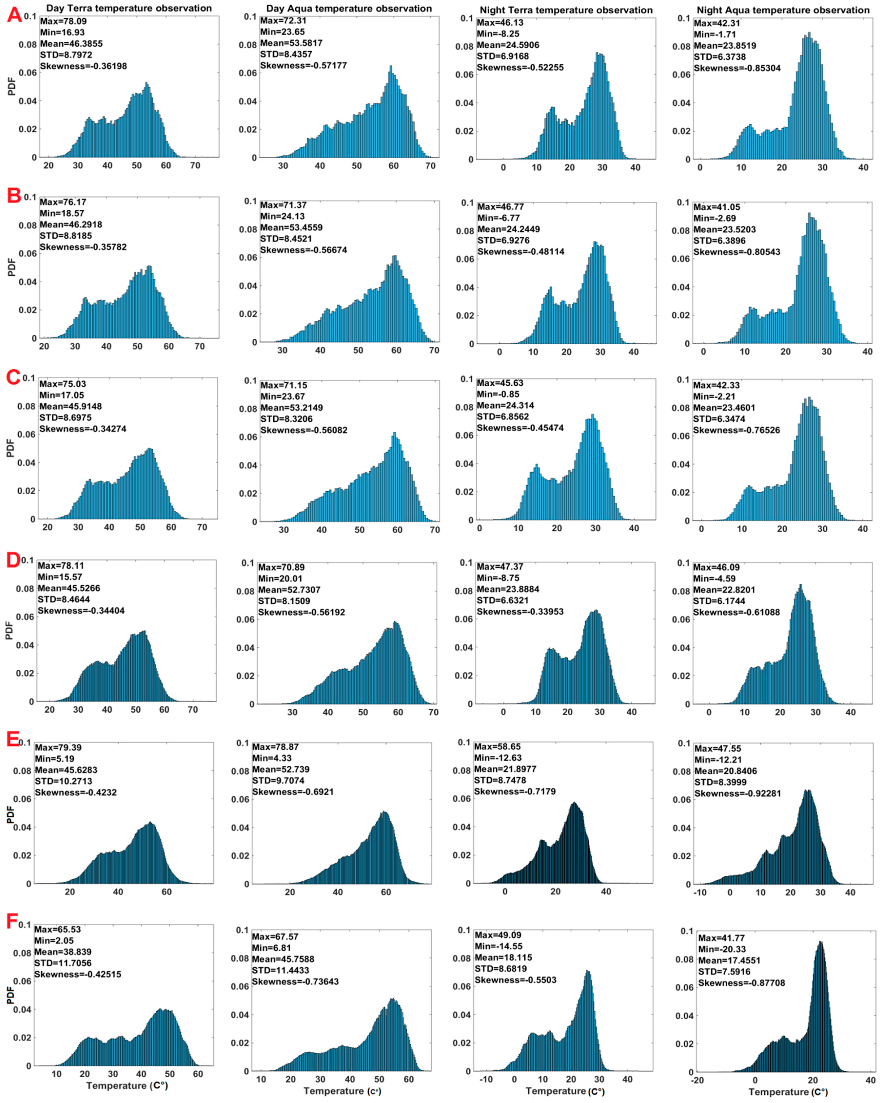
In order to have a better understanding of the LST variability in the six deserts, the LST values of the MODIS (four) observation times for the whole time series were plotted by histograms (Figure 6). The vertical axes of the histograms are the Probability Density Function (PDF) and the horizontal axes are temperature (°C). The histograms were arranged based on the time of observation (MOD-D, MYD-D, MOD-N, and MYD-N) from left to right for each desert. All of the histograms show a negative skewness, which indicates a higher occurrence of upper bounds of temperature at each observation time. The day and night ranges of LSTs in deserts for the whole time series were large: Rigzar [−8.25, 78.09] °C, Wahiba [−6.77, 76.17] °C, Kharan [−2.21, 75.03] °C, Registan [−8.75, 78.11] °C, Rub al Khali [−12.63, 79.39] °C, and An Nafud [−20.33, 65.57] °C. At each row, the mean LSTs increased with the time for daily observations and decreased for nightly observations; this showed that MYD-D observations were generally closer to the maximum daily LST and MYD-N were closer to the minimum nightly LST. The presented maximum LSTs at MOD-D were recorded on day 143 in 2015 (23 May), for which MYD-D data were not available. Considering the temporal variability of MOD11A1 and MYD11A1, and the data gap for some dates, it is not possible to measure the exact maximum and minimum LSTs with MODIS LST observation. STDs in MYD-D and MYD-N showed the lowest values for the day and night-time. It can be stated that the lowest STDs among the observation times occurred at the maximum and minimum diurnal LSTs. This is also obvious from the minimum and maximum LST values at each observation time; for MOD-D and MOD-N, the range of the minimum and maximum is larger than MYD-D and MYD-N. The reason for such behavior can be attributed to the constant upper and lower bounds of LST; before or after the minimum and maximum LST times, the variability of LSTs was larger. An analysis of shape, mean, STD, and skewness showed that Rigzar, Wahiba, Kharan, Registan, and Rub al Khali exhibited almost the same behavior at the four recorded times. The STDs of An Nafud at each observation time indicated a larger variability.
4.2. LST Difference of MODIS and INSAT
To implement temporal matching, the diurnal INSAT LST patterns for all pixels (Figure 7) in the study area deserts were constructed by the linear interpolation among half hourly data.
In the next step, to analyze the behavior of high LSTs, MOD-D and MYD-D LST observations were subtracted from interpolated INSAT LST observations for each pixel, from 10 April 2015 to 22 October 2016. The mean values of the LST differences (vertical axis) for the whole time series were plotted against five degree intervals (horizontal axis), from 30 °C to the maximum LST observations recorded by MODIS for the six deserts (Figure 8); the means were plotted between the upper and lower bounds of each five degree interval (for example, for 30–35, the plot is at 32.5 °C). This threshold was selected so that more than 20 pixels per bin were used and provides more robust results. The number of pixels at each interval is shown in Table 2 and Table 3. In MOD-D, the range of mean differences was between −4.3 and +11.16 °C. In MYD-D, the mean differences varied from −2.00 to +15.5 °C; higher LSTs in MYD-D showed larger mean differences (Rub Al Khali displayed the maximum mean differences). In both plots, the more the temperature increased, the more the mean LST differences increased in all deserts and the maximum value was reached at 78.87 °C. In both plots, An Nafud had a smaller slope. This means that the mean differences in An Nafud were smaller than in the other deserts. Such behavior may be attributed to the effect of VZA in this area. INSAT viewed this desert by VZA between 50 to 57 degrees and the MODIS VZA was between 44.5 and 62.5 (based on angular matching). It suggested that in higher VZAs, both sensors had lower LST changes in contrast with other deserts. The mean LST difference in the An Nafud desert started from near zero in 30 to 40 °C. In the MOD-D plot, the mean differences in Wahiba, Rub al Khali, and Registan changed sign in the 50–55 °C range, and in Kharan and Rigzar, the change of sign happened between 55–60 °C. In the MYD-D plot, in all deserts except for An Nafud, the mean differences changed sign at 50–55 °C. Minor differences may be attributed to normal discrepancies which exist between the two sensors in lower temperatures. After the sign change of the mean differences, they showed almost similar slopes (except for An Nafud), with some nuances.
As depicted in Figure 7, there were some fluctuations in the INSAT LST patterns. The oscillations can be produced by sensor noises and diverse environmental conditions. Moreover, the absence of INSAT LST observations at some points of time might generate gaps in linear interpolation. Therefore, it was essential that DTC models of the two sensors were constructed for an accurate analysis of the relationship between MODIS and INSAT LSTs, which were not concurrent in all observation times. For INSAT DTC modeling, all four variables (T0, Ta, , and tm) were estimated by fitting the equation to LST observations. ts, as the last part of the day model was regarded as a free variable with the least RMSE from INSAT LST observations for each pixel. In other words, a time period was defined as the searching space (two hours before sunset to two hours after sunset), and the ts with the least RMSE fitted to half hourly INSAT LSTs. When estimating the MODIS daytime DTC model, four parameters (T0, Ta, tm, and ) were unknown, and ts was regarded as 1 h before tss. Therefore, four MODIS observations can be used for an estimation of the unknown parameters. Figure 9 shows the sample estimated DTC models for both MODIS and INSAT pixels with high LSTs in the six study area deserts. When observing the DTCs, it becomes clear that for higher temperatures, the differences were higher. The four MODIS observation times caused some movements in the DTCs. Based on the described MYD-D variability and DTCs, it can be concluded that the MYD-D observation times are closer to tm. Along with the observed differences in high temperatures between MODIS and INSAT in all DTC models, INSAT and MODIS exhibited other differences. Since INSAT uses plenty of observations, it’s estimated that the DTC model could be better fitted to the observations, even when considering gapping data. In MODIS estimated DTCs, the applied mathematical model tries to fit the model to four observations and if any noise or substantial environmental changes happen at any observation time, it cannot present a high quality DTC model. In fact, it is highly dependent on four observations. As indicated in Figure 9, there existed some shifts in tm in all of the deserts. This proved that DTC in MODIS cannot consider changes in environmental conditions. One solution could be to use the parameters derived from INSAT DTC; calculated t0, tm, and k values can be used as controlling criteria in MODIS DTC, to improve the results.
5. Discussion
In this study, the differences between high LSTs from daily MODIS and INSAT observations were investigated in six deserts, with VZAs ranging between 37 to 57 degrees. In the first step, the variability of LSTs in the six deserts was analyzed for the whole time series. The observed LSTs at each observation time showed that MYD-D is closer to the maximum diurnal LST. The highest LSTs were recorded in Rub al Khali, Kharan, and Rigzar. It is worth noting that the retrieved high LSTs were larger than the declared LSTs in [28], which could be the result of using modified LST V6. Therefore, to analyze the highest LSTs on earth, a comprehensive study over a long period of time is needed. One solution for estimating the maximum diurnal LST is applying DTC models and estimating Ta. The STDs of all observation times showed a dependency on time and temperature; the STDs in the MOD observations were larger than MYD, which included the highest and lowest temperatures. The results of the mean differences between spatially, temporally, and geometrically matched MODIS and INSAT LSTs in the applied dataset indicated a positive increasing trend for both MOD-D and MYD-D observations with a temperature increase. The differences grew from zero degrees to about +11 °C for MOD-D, and +15 °C for MYD-D in high LSTs; this showed that the measure of discrepancies was a function of temperature. All deserts except for An Nafud showed almost the same trends of discrepancies in connection with a temperature increase. The lower slopes in An Nafud can be attributed to the effect of higher VZAs. Due to the temporal variability of the MOD11A1 and MYD11A1 products, and environmental and sensor noises and data gaps, some fluctuations occurred in INSAT LST diurnal patterns, which made the comparison difficult. In order to analyze the behaviors of both sensors in a continuous space, DTC models were applied. Sample DTC models for the six deserts also showed the discrepancies of MODIS and INSAT in high temperatures. In addition to the observed discrepancies in high temperatures, some discrepancies (such as the difference in the tm estimation) were observed between MODIS and INSAT DTCs. Due to the low number of MODIS observations, any changes in LST at one observation time (by environmental condition or sensor noise) could change the shape of the whole fitted DTC. Mainly, such differences happen in t0, tm, and k estimations. Since the INSAT DTC model used plenty of observations for estimating the parameters, it could consider the LST changes between MODIS observations. In fact, it would be possible to use the three mentioned parameters in the INSAT DTC as controlling criteria in MODIS DTC fitting, to increase the accuracy. A portion of the observed discrepancies in high temperatures can be attributed to calibration differences and sensor noise, which also exists in lower temperatures. Other reasons for such discrepancies may be expressed by different LST retrieval algorithms in INSAT and MODIS, as follows: (1) in both sensors, different equations were applied for LST retrieval; (2) in MODIS, different ranges were considered for parameters in MODTRAN simulations to calculate the coefficients in the equations; for MODIS, the atmospheric boundary layer temperature range is between 257 and 325 K, but for INSAT, it ranges from 260–320 K. The MODIS LST ranges between 265 and 354 K, whereas the INSAT LST is between 260 and 330 K. The MODIS emissivity data were from MODIS daily products, while with INSAT, monthly MODIS emissivity values were applied. In MODIS, eight angle bins were used to compensate for dictated VZA effects, in comparison to the seven applied by INSAT. The authors propose that such discrepancies were the result of all of the mentioned differences in LST retrieval for both sensors. They believe that by conducting a forward-backward method and changing the input parameters, it would be possible to determine the exact effect of each parameter in the observed discrepancies in high LSTs.
6. Conclusions
The results of this study showed considerable discrepancies between INSAT and daily MODIS (especially in MYD-D) LST observations for high temperatures in six sandy deserts. The authors have proposed that the nature of such discrepancies may be attributed to the differences in the LST retrieval algorithms for both sensors. This study demonstrated the application of DTC models for the analysis of LST discrepancies in a continuous space. It is proposed that the possibility of modeling LST discrepancies between geostationary and polar satellites in a continuous space using DTC models could be investigated in future studies. An analysis of LST variability in this study indicated high LSTs in the studied deserts. An investigation of high LSTs, in 8–10 μm excluding the Ozone absorption spectrum, demands particular attention; when the temperature increases, the wavelength of maximum radiance is decreased. According to Wien’s displacement law, the maximum emission decreases when the temperature increases. For a temperature range between 250 K and 330 K, this wavelength changes between 11.6 μm to 8.8 μm. According to Li et al. [22], the average temperature of the Earth is approximately 288 K, but for higher temperatures like 340 K, the maximum radiating wavelength is 8.5 μm. Future studies using shorter wavelengths to study this concept are required. Upcoming hyperspectral infrared satellites like Hyperspectral Infrared INSAT (HyspIRI) can be of great help to study high LSTs with more accuracy. It is recommended that further research be conducted to examine the non-linearity of the Planck function used for LST retrieval in high temperature areas, by applying in situ measurements. For conducting comprehensive studies in this respect and other related disciplines, the Lut and Rub Al Khali (with high recorded LSTs) deserts can be good candidates. These regions have diverse, vast, and intact homogeneous land covers, low soil moisture, high and long term irradiance, low vegetation cover, low elevation fluctuations, a low number of cloudiness days, high latent heat flux, and are far from anthropogenic and natural pollutants. Since the effects of complicating variables in satellite sensor calibration were reduced, they are suitable areas for the validation of satellite LSTs using in situ measurements. By constructing more ground measurement stations, these areas have the potential to be developed into a laboratory to answer many issues in meteorology, climatology, and hydrology.
Acknowledgments
The authors would like to acknowledge NASA/USGS and the Meteorological and Oceanographic Satellite Data Archival Centre (MOSDAC) for providing access to the MOD11A1 product and INSAT3-D LST products. The authors deeply thank the Iranian National Science foundation and Iranian National Space Administration for their great support in conducting this research.
Author Contributions
Based on his multiple field observations from the study area, Seyed Kazem Alavipanah designed and conducted the research; Qihao Weng improved the technical analysis and finished the revision and submission of the paper; Mehdi Gholamnia downloaded the data and performed the analysis; Reza Khandan managed the research and wrote the first draft. All authors contributed to and approved the final manuscript.
Conflicts of Interest
The authors declare no conflict of interest.
References
- Sellers, P.; Hall, F.; Asrar, G.; Strebel, D.; Murphy, R. The first ISLSCP field experiment (FIFE). Bull. Am. Meteorol. Soc. 1988, 69, 22–27. [Google Scholar] [CrossRef]
- Wan, Z.; Wang, P.; Li, X. Using MODIS land surface temperature and normalized difference vegetation index products for monitoring drought in the southern Great Plains, USA. Int. J. Remote Sens. 2004, 25, 61–72. [Google Scholar] [CrossRef]
- Mackaro, S.M.; McNider, R.T.; Biazar, A.P. Some physical and computational issues in land surface data assimilation of satellite skin temperatures. Pure Appl. Geophys. 2012, 169, 401–414. [Google Scholar] [CrossRef]
- Park, S.K.; Xu, L. Data Assimilation for Atmospheric, Oceanic and Hydrologic Applications; Springer Science & Business Media: Berlin, Germany, 2013; Volume 2. [Google Scholar]
- Qin, J.; Liang, S.; Liu, R.; Zhang, H.; Hu, B. A weak-constraint-based data assimilation scheme for estimating surface turbulent fluxes. IEEE Geosci. Remote Sens. Lett. 2007, 4, 649–653. [Google Scholar] [CrossRef]
- Rodell, M.; Houser, P.; Jambor, U.; Gottschalck, J.; Mitchell, K.; Meng, C.; Arsenault, K.; Cosgrove, B.; Radakovich, J.; Bosilovich, M. The global land data assimilation system. Bull. Am. Meteorol. Soc. 2004, 85, 381–394. [Google Scholar] [CrossRef]
- Reichle, R.H.; Kumar, S.V.; Mahanama, S.P.; Koster, R.D.; Liu, Q. Assimilation of satellite-derived skin temperature observations into land surface models. J. Hydrometeorol. 2010, 11, 1103–1122. [Google Scholar] [CrossRef]
- Yao, Z.; Li, J.; Li, J.; Zhang, H. Surface emissivity impact on temperature and moisture soundings from hyperspectral infrared radiance measurements. J. Appl. Meteorol. Climatol. 2011, 50, 1225–1235. [Google Scholar] [CrossRef]
- Aires, F.; Prigent, C.; Rossow, W.; Rothstein, M.; Hansen, J.E. A new neural network approach including first-guess for retrieval of atmospheric water vapor, cloud liquid water path, surface temperature and emissivities over land from satellite microwave observations. Pap. Clim. Dyn. 2000. [Google Scholar] [CrossRef]
- Wan, Z.; Zhang, Y.; Zhang, Q.; Li, Z.-L. Quality assessment and validation of the MODIS global land surface temperature. Int. J. Remote Sens. 2004, 25, 261–274. [Google Scholar] [CrossRef]
- Wang, K.; Wang, P.; Li, Z.; Cribb, M.; Sparrow, M. A simple method to estimate actual evapotranspiration from a combination of net radiation, vegetation index, and temperature. J. Geophys. Res. Atmos. 2007, 112, D15. [Google Scholar] [CrossRef]
- Anderson, M.; Norman, J.; Diak, G.; Kustas, W.; Mecikalski, J. A two-source time-integrated model for estimating surface fluxes using thermal infrared remote sensing. Remote Sens. Environ. 1997, 60, 195–216. [Google Scholar] [CrossRef]
- French, A.; Schmugge, T.; Ritchie, J.; Hsu, A.; Jacob, F.; Ogawa, K. Detecting land cover change at the Jornada Experimental Range, New Mexico with ASTER emissivities. Remote Sens. Environ. 2008, 112, 1730–1748. [Google Scholar] [CrossRef]
- Jin, M. Analysis of land skin temperature using AVHRR observations. Bull. Am. Meteorol. Soc. 2004, 85, 587–600. [Google Scholar] [CrossRef]
- Karnieli, A.; Agam, N.; Pinker, R.T.; Anderson, M.; Imhoff, M.L.; Gutman, G.G.; Panov, N.; Goldberg, A. Use of NDVI and land surface temperature for drought assessment: Merits and limitations. J. Clim. 2010, 23, 618–633. [Google Scholar] [CrossRef]
- Lambin, E.; Ehrlich, D. The surface temperature-vegetation index space for land cover and land-cover change analysis. Int. J. Remote Sens. 1996, 17, 463–487. [Google Scholar] [CrossRef]
- Lensky, I.M.; Dayan, U. Satellite observations of land surface temperature patterns induced by synoptic circulation. Int. J. Climatol. 2015, 35, 189–195. [Google Scholar] [CrossRef]
- Luyssaert, S.; Jammet, M.; Stoy, P.C.; Estel, S.; Pongratz, J.; Ceschia, E.; Churkina, G.; Don, A.; Erb, K.; Ferlicoq, M. Land management and land-cover change have impacts of similar magnitude on surface temperature. Nat. Clim. Chang. 2014, 4, 389–393. [Google Scholar] [CrossRef]
- Matsui, T.; Lakshmi, V.; Small, E. Links between snow cover, surface skin temperature, and rainfall variability in the North American monsoon system. J. Clim. 2003, 16, 1821–1829. [Google Scholar] [CrossRef]
- Vose, R.S.; Arndt, D.; Banzon, V.F.; Easterling, D.R.; Gleason, B.; Huang, B.; Kearns, E.; Lawrimore, J.H.; Menne, M.J.; Peterson, T.C. NOAA’s merged land–ocean surface temperature analysis. Bull. Am. Meteorol. Soc. 2012, 93, 1677–1685. [Google Scholar] [CrossRef]
- Holmes, T.; Owe, M.; De Jeu, R.; Kooi, H. Estimating the soil temperature profile from a single depth observation: A simple empirical heatflow solution. Water Resour. Res. 2008, 44. [Google Scholar] [CrossRef]
- Li, Z.-L.; Tang, B.-H.; Wu, H.; Ren, H.; Yan, G.; Wan, Z.; Trigo, I.F.; Sobrino, J.A. Satellite-derived land surface temperature: Current status and perspectives. Remote Sens. Environ. 2013, 131, 14–37. [Google Scholar] [CrossRef]
- Trigo, I.F.; Monteiro, I.T.; Olesen, F.; Kabsch, E. An assessment of remotely sensed land surface temperature. J. Geophys. Res. Atmos. 2008, 113, D17. [Google Scholar] [CrossRef]
- Gao, C.; Jiang, X.; Wu, H.; Tang, B.; Li, Z.; Li, Z.-L. Comparison of land surface temperatures from MSG-2/SEVIRI and Terra/MODIS. J. Appl. Remote Sens. 2012, 6. [Google Scholar] [CrossRef]
- Qian, Y.-G.; Li, Z.-L.; Nerry, F. Evaluation of land surface temperature and emissivities retrieved from MSG/SEVIRI data with MODIS land surface temperature and emissivity products. Int. J. Remote Sens. 2013, 34, 3140–3152. [Google Scholar] [CrossRef]
- Cho, A.-R.; Suh, M.-S. Evaluation of land surface temperature operationally retrieved from Korean geostationary satellite (COMS) data. Remote Sens. 2013, 5, 3951–3970. [Google Scholar] [CrossRef]
- Duan, S.-B.; Li, Z.-L. Intercomparison of operational land surface temperature products derived from MSG-SEVIRI and Terra/Aqua-MODIS data. IEEE J. Sel. Top. Appl. Earth Obs. Remote Sens. 2015, 8, 4163–4170. [Google Scholar] [CrossRef]
- Mildrexler, D.J.; Zhao, M.; Running, S.W. Satellite finds highest land skin temperatures on earth. Bull. Am. Meteorol. Soc. 2011, 92, 855–860. [Google Scholar] [CrossRef]
- Wan, Z. New refinements and validation of the collection-6 MODIS land-surface temperature/emissivity products. Remote Sens. Environ. 2014, 140, 36–45. [Google Scholar] [CrossRef]
- Wan, Z.; Dozier, J. A generalized split-window algorithm for retrieving land-surface temperature from space. IEEE Trans. Geosci. Remote Sens. 1996, 34, 892–905. [Google Scholar]
- Wan, Z. MODIS Land Surface Temperature Products Users’ Guide; Institute for Computational Earth System Science, University of California: Santa Barbara, CA, USA, 2006. [Google Scholar]
- Snyder, W.C.; Wan, Z.; Zhang, Y.; Feng, Y.-Z. Classification-based emissivity for land surface temperature measurement from space. Int. J. Remote Sens. 1998, 19, 2753–2774. [Google Scholar] [CrossRef]
- EPSA. INSAT-3D Algorithm Theoretical Basis Document; Space Applications Centre, Government of India: Umiam, India, 2015; p. 379.
- Hewison, T.J.; Wu, X.; Yu, F.; Tahara, Y.; Hu, X.; Kim, D.; Koenig, M. GSICS inter-calibration of infrared channels of geostationary imagers using Metop/IASI. IEEE Trans. Geosci. Remote Sens. 2013, 51, 1160–1170. [Google Scholar] [CrossRef]
- Inamdar, A.K.; French, A.; Hook, S.; Vaughan, G.; Luckett, W. Land surface temperature retrieval at high spatial and temporal resolutions over the southwestern United States. J. Geophys. Res. Atmos. 2008, 113, D7. [Google Scholar] [CrossRef]
- Elagib, N.A.; Alvi, S.H.; Mansell, M.G. Day-length and extraterrestrial radiation for Sudan: A comparative study. Int. J. Sol. Energy 1999, 20, 93–109. [Google Scholar] [CrossRef]
- Duan, S.-B.; Li, Z.-L.; Tang, B.-H.; Wu, H.; Tang, R.; Bi, Y.; Zhou, G. Estimation of diurnal cycle of land surface temperature at high temporal and spatial resolution from clear-sky MODIS data. Remote Sens. 2014, 6, 3247–3262. [Google Scholar] [CrossRef]
- Duan, S.-B.; Li, Z.-L.; Wang, N.; Wu, H.; Tang, B.-H. Evaluation of six land-surface diurnal temperature cycle models using clear-sky in situ and satellite data. Remote Sens. Environ. 2012, 124, 15–25. [Google Scholar] [CrossRef]
Figure 1.
Six study area deserts. Blue contour lines are the VZA of INSAT and the violet boxes are MODIS tiles (Image source: Google Earth).
Figure 1.
Six study area deserts. Blue contour lines are the VZA of INSAT and the violet boxes are MODIS tiles (Image source: Google Earth).
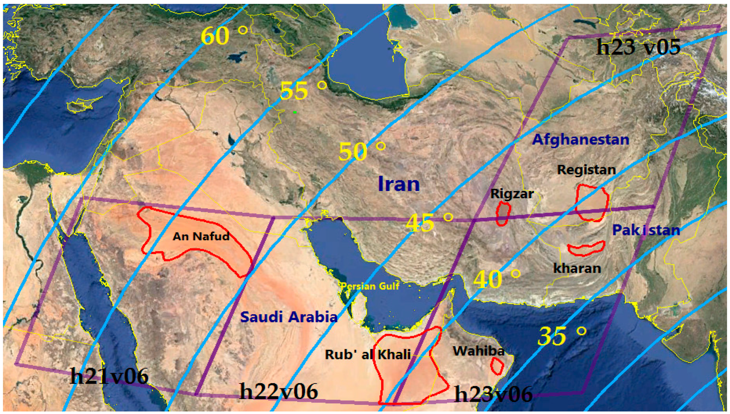
Figure 2.
Emissivity of six study area deserts in August 2015 based on the MOD11C3 product.
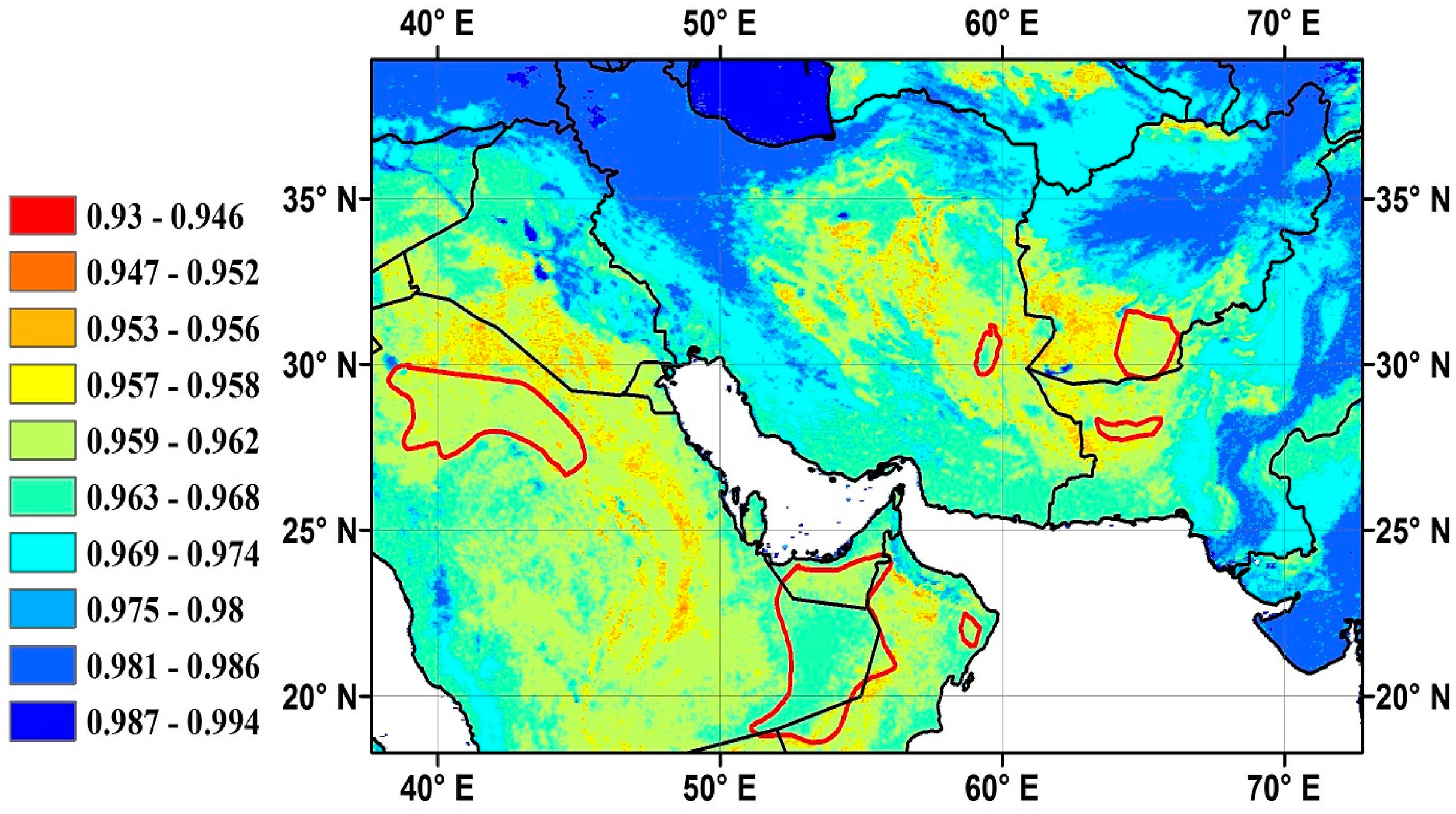
Figure 3.
Spectral response of MODIS bands 31 and 32 and INSAT TIR bands (NASA Langley Cloud and Radiation Research Group).
Figure 3.
Spectral response of MODIS bands 31 and 32 and INSAT TIR bands (NASA Langley Cloud and Radiation Research Group).
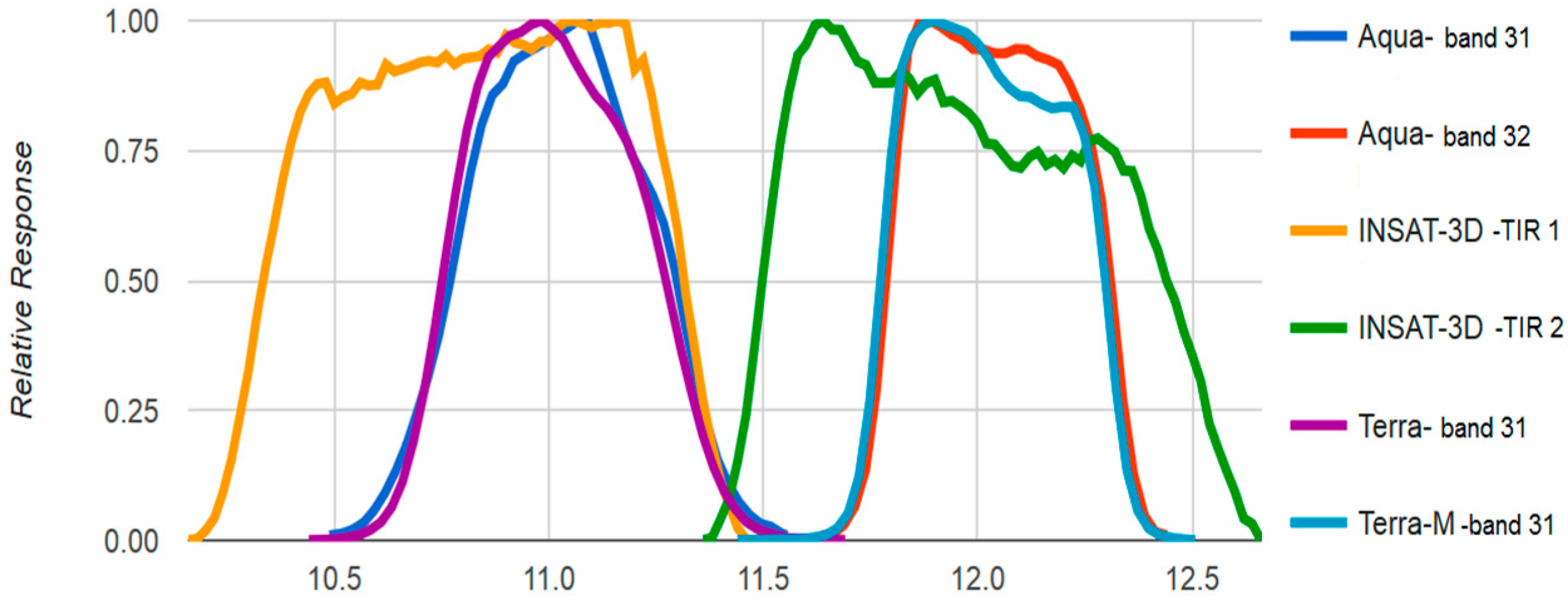
Figure 4.
Flowchart of MODIS and INSAT LST comparison for high temperatures using DTC models.
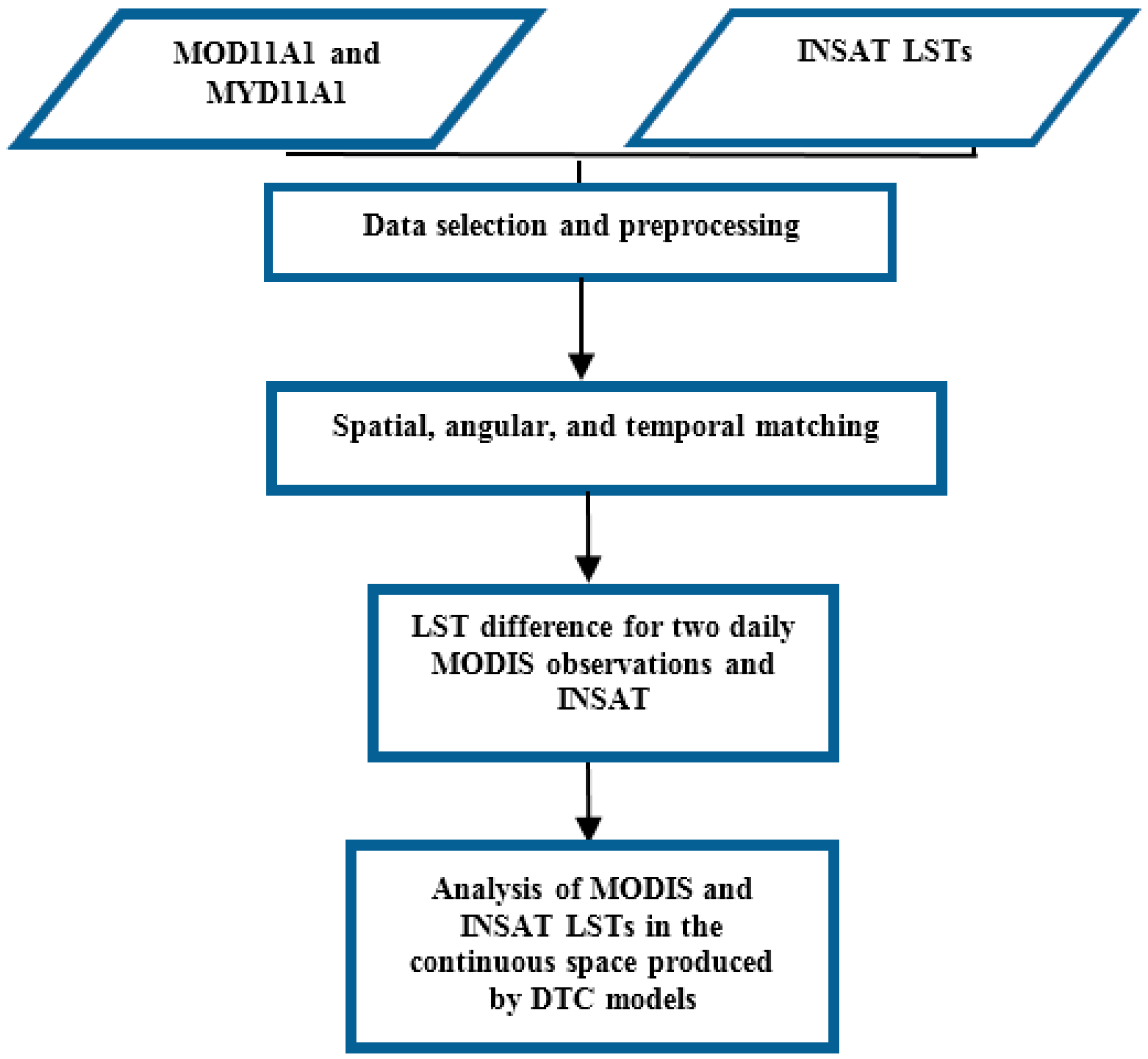
Figure 5.
DTC model parameters [37].
Figure 5.
DTC model parameters [37].
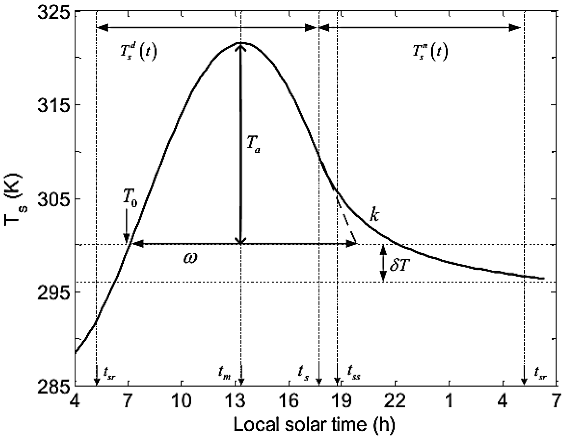
Figure 6.
Variability of LSTs in the study area deserts derived from MODIS at four observation times. On the upper left corner of each histogram maximum, minimum, mean, STD, and skewness were displayed. Rows (A–F) show the histograms for Rigzar, Wahiba, Kharan, Regisatn, Rub’ al Khali, and An Nafud, respectively.

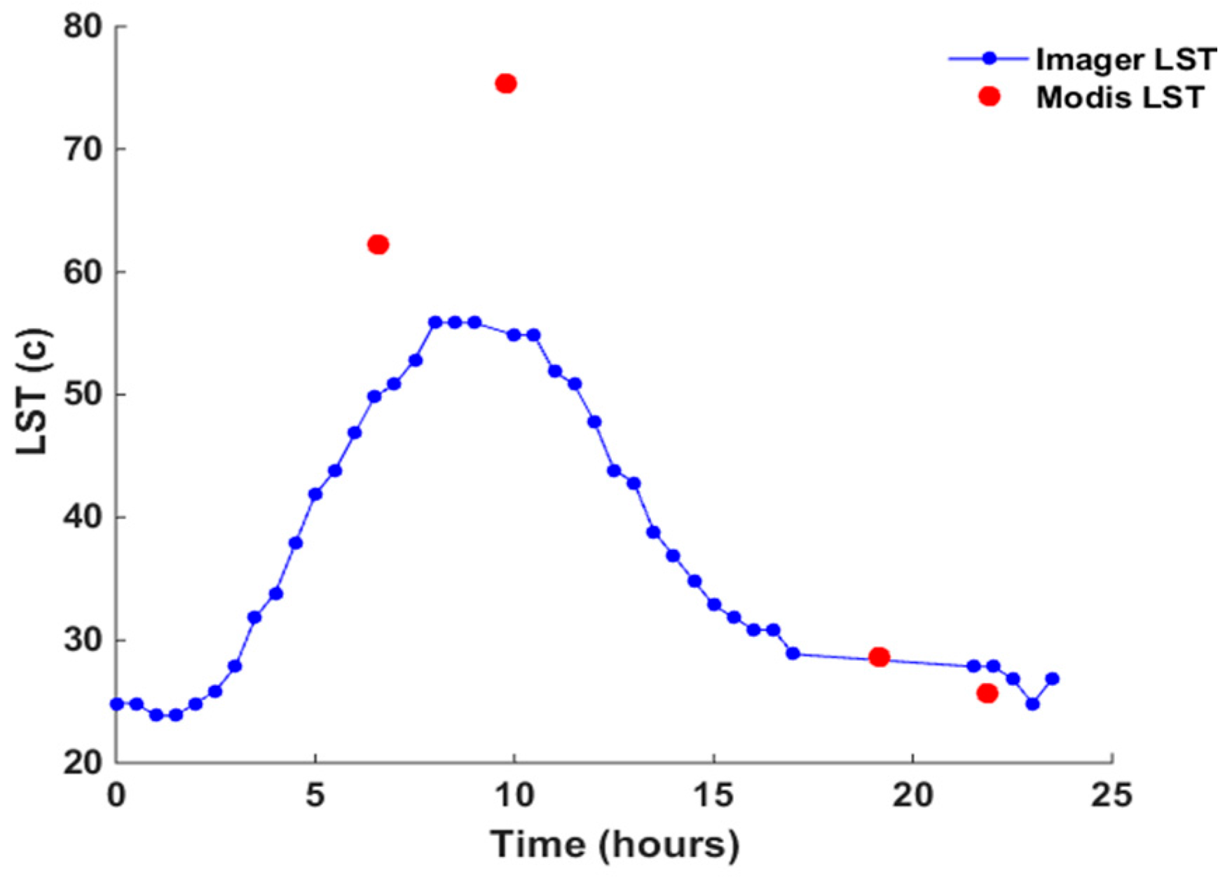
Figure 7.
Diurnal LST pattern of INSAT data (blue line) plotted against MODIS observations (red dots) for a sample pixel.
Figure 7.
Diurnal LST pattern of INSAT data (blue line) plotted against MODIS observations (red dots) for a sample pixel.

Figure 8.
The histograms of the mean LST differences ([MODIS − INSAT LST]) for the study areas. (A) MOD-D difference with INSAT; (B) MYD-D difference with INSAT.
Figure 8.
The histograms of the mean LST differences ([MODIS − INSAT LST]) for the study areas. (A) MOD-D difference with INSAT; (B) MYD-D difference with INSAT.
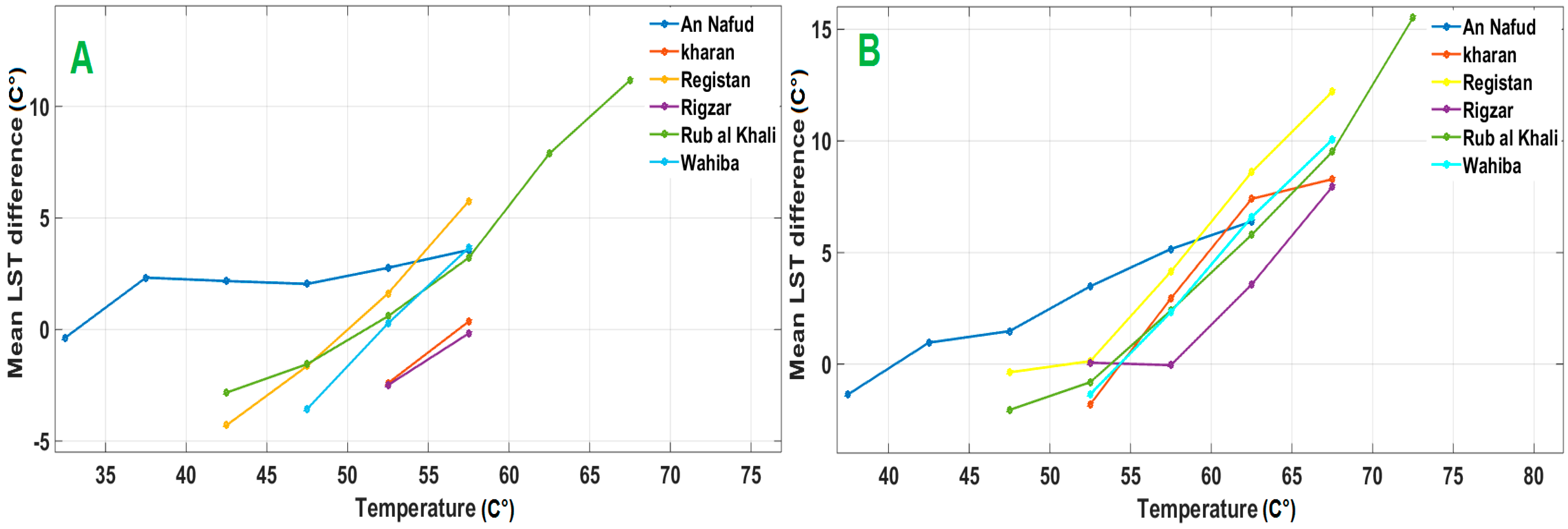
Figure 9.
Sample DTCs for six pixels in the study area deserts with high LSTs in 2016 (locations of pixels and DOY was written above each figure). Black DTCs are from MODIS and purple DTCs are from INSAT, and dots show the MODIS and INSAT observation per day.
Figure 9.
Sample DTCs for six pixels in the study area deserts with high LSTs in 2016 (locations of pixels and DOY was written above each figure). Black DTCs are from MODIS and purple DTCs are from INSAT, and dots show the MODIS and INSAT observation per day.


Table 1.
Comparison of specifications for LST retrieval in MODIS and INSAT.
| Parameters | MODIS | INSAT-3D |
|---|---|---|
| Radiative transfer model | MODTRAN4 | MODTRAN4 |
| atmospheric surface boundary layer temperature range | 280–325 K for daytime 275–305 K for nighttime Total range: 275–325 K | 260 and 320 K |
| LST range | 288 and 354 K daytime 265 and 309 K nighttime Total range: 265–354 K | 260–330 K |
| water vapor | almost near zero to 5.5 cm | 0.1 g/cm2 to near saturated level (5 g/cm2 ) |
| VZA | 8 bins | 7 bins (0–20, 20–32.5, 32.5–37.5, 37.5–42.5, 42.5–47.5, 47.5–52.5, 52.5 and above). |
| Emissivity | MODIS emissivity product | MODIS emissivity product |
Table 2.
Number of pixels at each five degree interval in [MOD-D − INSAT] for calculating the mean differences.
Table 2.
Number of pixels at each five degree interval in [MOD-D − INSAT] for calculating the mean differences.
| MOD-D | 30–35 | 35–40 | 40–45 | 45–50 | 50–55 | 55–60 | 60–65 | 65–70 |
|---|---|---|---|---|---|---|---|---|
| An Nafud | 20 | 1459 | 7742 | 23021 | 30466 | 11687 | 0 | 0 |
| Kharan | 0 | 0 | 0 | 0 | 200 | 218 | 0 | 0 |
| Registan | 0 | 0 | 22 | 565 | 1417 | 846 | 0 | 0 |
| Rigzar | 0 | 0 | 0 | 0 | 515 | 366 | 0 | 0 |
| Rub al Khali | 0 | 0 | 129 | 2731 | 11536 | 15413 | 5085 | 1288 |
| Wahiba | 0 | 0 | 0 | 22 | 183 | 173 | 0 | 0 |
Table 3.
Number of pixels at each five degree interval in [MYD-D − INSAT] for calculating the mean differences.
Table 3.
Number of pixels at each five degree interval in [MYD-D − INSAT] for calculating the mean differences.
| MYD | 30–35 | 35–40 | 40–45 | 45–50 | 50–55 | 55–60 | 60–65 | 65–70 | 70–75 |
|---|---|---|---|---|---|---|---|---|---|
| An Nafud | 0 | 98 | 1652 | 10277 | 35260 | 47121 | 4613 | 0 | 0 |
| Kharan | 0 | 0 | 0 | 0 | 153 | 577 | 781 | 94 | 0 |
| Regisatan | 0 | 0 | 0 | 247 | 2684 | 6827 | 8065 | 777 | 0 |
| Rigzar | 0 | 0 | 0 | 0 | 92 | 1083 | 1865 | 465 | 0 |
| Rub al Khali | 0 | 0 | 0 | 1341 | 7822 | 17173 | 20420 | 5131 | 817 |
| Wahiba | 0 | 0 | 0 | 0 | 106 | 245 | 660 | 159 | 0 |
© 2017 by the authors. Licensee MDPI, Basel, Switzerland. This article is an open access article distributed under the terms and conditions of the Creative Commons Attribution (CC BY) license (http://creativecommons.org/licenses/by/4.0/).
Share and Cite
MDPI and ACS Style
Alavipanah, S.K.; Weng, Q.; Gholamnia, M.; Khandan, R. An Analysis of the Discrepancies between MODIS and INSAT-3D LSTs in High Temperatures. Remote Sens. 2017, 9, 347. https://doi.org/10.3390/rs9040347
AMA Style
Alavipanah SK, Weng Q, Gholamnia M, Khandan R. An Analysis of the Discrepancies between MODIS and INSAT-3D LSTs in High Temperatures. Remote Sensing. 2017; 9(4):347. https://doi.org/10.3390/rs9040347
Chicago/Turabian StyleAlavipanah, Seyed Kazem, Qihao Weng, Mehdi Gholamnia, and Reza Khandan. 2017. "An Analysis of the Discrepancies between MODIS and INSAT-3D LSTs in High Temperatures" Remote Sensing 9, no. 4: 347. https://doi.org/10.3390/rs9040347
Note that from the first issue of 2016, this journal uses article numbers instead of page numbers. See further details here.