
Automatic Estimation of Tree Position and Stem Diameter Using a Moving Terrestrial Laser Scanner


1
Faculty of Science and Technology, Norwegian University of Life Sciences, 1432 Ås, Norway
2
Faculty of Environmental Sciences and Natural Resource Management, Norwegian University of Life Sciences, 1432 Ås, Norway
*
Author to whom correspondence should be addressed.
Remote Sens. 2017, 9(4), 350; https://doi.org/10.3390/rs9040350
Submission received: 15 February 2017
/
Revised: 26 March 2017
/
Accepted: 1 April 2017
/
Published: 6 April 2017
Abstract
:Airborne laser scanning is now widely used for forest inventories. An essential part of inventory is a collection of field reference data including measurements of tree stem diameter at breast height (DBH). Traditionally this is acquired through manual measurements. The recent development of terrestrial laser scanning (TLS) systems in terms of capacity and weight have made these systems attractive tools for extracting DBH. Multiple TLS scans are often merged into a single point cloud before the information extraction. This technique requires good position and orientation accuracy for each scan location. In this study, we propose a novel method that can operate under a relatively coarse positioning and orientation solution. The method divides the laser measurements into limited time intervals determined by the laser scan rotation. Tree positions and DBH are then automatically extracted from each laser scan rotation. To improve tree identification, the estimated center points are subsequently processed by an iterative closest point algorithm. In a small reference data set from a single field plot consisting of 18 trees, it was found that 14 were automatically identified by this method. The estimated DBH had a mean differences of 0.9 cm and a root mean squared error of 1.5 cm. The proposed method enables fast and efficient data acquisition and a 250 m2 field plot was measured within 30 s.
1. Introduction
Forest inventories are of paramount importance for sustainable and effective management of forest resources. Airborne laser scanning (ALS) is now widely used in forest inventories [1]. An essential part of forest inventories based on ALS is field reference data collection. Field data are typically acquired by manual measurements on circular sample plots of 200–400 m2 in size distributed over the landscape in question according to statistically rigorous sampling principles [2]. The use of terrestrial laser scanning (TLS) to acquire field reference data in these ALS-based forest inventories has been proposed. In a recent review study by Liang et al. [3] it is acknowledged that there is a potential for utilization of TLS in forest inventories. A TLS system uses a laser to measure distances in a regular pattern around the scanner. This information is used to create a dense point cloud covering the surroundings of the scanner position. A setup where the scanner position is fixed is often referred to as a static TLS. If the scanner moves during data capture, the system can be referred to as a kinematic TLS.
There are several studies providing methods for highly detailed description of single trees from single or multiple scanning positions in the field, often including all branches and leaves [4,5]. Tree architecture modeling has been used for biomass estimation [6,7,8] and forest structure description [9] at the plot or single tree level.
The use of TLS for the acquisition of specific biophysical tree parameters has been investigated in several studies, including estimation on diameter at breast height (stem diameter at 1.3 m above ground level; DBH) and tree stem volume [10,11,12,13,14,15]. A full or partial reconstruction of individual trees has also been investigated [5,16,17,18,19]. Direct estimation of single tree biomass from TLS data has been described in [6,8]. Others have estimated biomass from TLS data through tree stem reconstruction [20] or by using related TLS-estimates with existing allometric models [15,21].
Yang et al. [9] used multiple scans in individual field plots and found good agreement between field reference DBH, tree heights, and number of trees and corresponding properties derived from the TLS data. Positioning field plots using global navigation satellite system (GNSS) in forests can be affected by unfavorable conditions for reception of satellite signals, and reliably obtaining an accurate geo-referenced position typically requires a survey-grade GNSS receiver [22]. As an alternative to GNSS positioning of field plots and trees in the field, Hauglin et al. [23] demonstrated that the ALS data that exist in many forest inventory projects can be used together with TLS data for positioning purposes by matching ALS and TLS data and exploiting the inherent absolute positions of the ALS data. Both the use of multiple TLS scans and the use of a single scan—the latter typically acquired from the plot center—have been proposed. By using only a single scan, the data acquisition and post-processing procedures are greatly simplified and the acquisition time is reduced [24,25,26]. The main challenge in using a single scan setup is to handle the tree shadows that will occur in the TLS data. This is acknowledged in previous studies [12,27]. Depending on the tree density and factors such as the presence of undergrowth and low branches, a number of trees will be occluded from the view of the scanner and hence cannot be detected. Automated detection algorithms are in practice associated with omission and commission errors, which means that some trees visible from the scanner will go undetected and that some patterns in the data occasionally will cause the algorithm to detect trees that are actually not present. For these reasons, some of the trees within a field plot will often not be detected from a single TLS scan. Liang et al. [28] reviewed several previous studies and reported that 10–32% of the trees were reported to be occluded from the plot center, depending on tree density and plot size. In the same studies, an additional 4–33% of the visible trees were not detected, depending on the algorithm that was applied and other factors. Tree occlusion and handling of omission errors when using multiple scanning positions were the main objectives of the studies [29,30]. Astrup et al. [31] tested several approaches to estimating a corrected stand volume, taking into account the omitted trees. They found that without a correction the volume was substantially underestimated using single-scan TLS data. When applying a statistically founded correction, they obtained results which were closer to the volume computed from field measurements, but differences could still be observed. This suggests that it could be beneficial to investigate other methods to handle or avoid tree occlusion.
Time consumption is an important factor when considering the use of TLS on forest field plots. Bauwens et al. [32] noted that a plot typically can be measured within 10 min with a single static scan setup. The use of multiple scan locations in order to reduce occlusion will substantially increase the time needed for each plot.
As an alternative to the use of multiple static scanner positions, the problem of occlusion can be eliminated by moving the scanner while scanning, typically referred to as mobile laser scanning. A few studies have described the application of this technique in forests. Forsman et al. [33] used a laser scanner and cameras mounted on a car to measure trees along a forest road. Bauwens et al. [32] used a wearable rig consisting of a TLS scanner and additional sensors such as a GNSS receiver and an inertial measurement unit (IMU), which can be referred to as a kinematic TLS system. Walking with this rig through the forest produced a point cloud from which positions and other single tree properties could be derived. Bauwens et al. [32] and Ryding et al. [34] used a hand-held laser scanner with an integrated IMU to produce similar point clouds by walking through a forest area with the scanner.
In these and other studies, point cloud data are typically captured from multiple positions and merged prior to a feature extraction such as detection of tree stems. Accurate position and orientation are needed in order to merge multiple scans, and lack of accuracy will produce noisy point clouds due to errors when aligning data captured from different positions. In the present study, we propose a novel approach by which point data from as little as a single scanner rotation of a moving laser scanner is used for tree stem detection. In the current set-up of the method, a scanner rotation typically would take 0.05 s. This approach ensures that a spatially consistent point cloud is used for tree stem detection, and could form the basis for simultaneous localization and mapping (SLAM) using the detected trees. Thus, the aim of the current study was to develop and implement the proposed method and test it in a real forest environment by assessing the obtained accuracy of tree detection, tree position, and estimated DBH.
2. Instrumentation and Data Collection
2.1. Study Area and Field Reference Data Collection
The study area is located in Gran municipality in southeastern Norway (60°27’ N 10°33’ E, 500 m above sea level). The forest in Gran is boreal and dominated by Norway spruce (Picea abies (L.) Karst.) and Scots pine (Pinus sylvestris L.). An existing circular sample plot of 250 m2 in a pine-dominated forest stand was subjectively selected from a dataset collected as part of another research project in the area. The plot was measured in field in August 2015. At the plot, all trees with a DBH >4 cm were accurately positioned, using an SOKKIA SET5 total station with additional measurements to at least two known points. The position of the two known points was obtained by post-processed GNSS baselines with base station data obtained from the Norwegian Mapping Authority. The receiver logged satellite data for more than 30 min. For all positioned trees, the DBH and species were also registered. The individual tree stems were calipered for diameter only once (a single measurement). In Table 1 a summary of the trees in the sample plot is given.
2.2. ALS Data Acquisition
The present study took advantage of ALS data acquired as part of an operational stand-based forest inventory. The ALS data were acquired on June 2015 with a Leica ALS70 sensor mounted on a fixed-wing aircraft, and the mean point density of the acquired ALS data was five points per m2. The ALS echoes were classified into “ground” and “non-ground” points by the data provider using the TerraScan software (Version 015, Terrasolid: Kanavaranta, Finland) [35]. From the ALS points classified as ground points, a triangular irregular network (TIN) was created to represent the terrain surface height. The vertical accuracy of the surface model was expected to be approximately 20–30 cm [36]. Only the ALS echoes classified as ground points were used in the present study.
2.3. TLS Data Acquisition
TLS data were collected on the sample plot in April 2016 using an instrumentation integrating three primary components. The three hardware components used are illustrated in Figure 1. The VLP16 from Velodyne [37] was used as the terrestrial laser scanner. This instrument can be referred to as a low-cost laser scanner compared to traditional TLS systems. All laser measurements were timestamped with GPS time during data capture. The Velodyne VLP16 laser scanner has 16 individual laser beams rotating around the z-axis. The rotation speed is 5–20 rotations per second, referred to as scan rate. The vertical angle distance between each beam is 2 degrees. This gives a total field of view of 30 × 360 degrees. In this project, the pulse repetition rate was 300 kHz and the scan rate was 20 Hz. The data were stored and exported with VeloView v3.1.1.
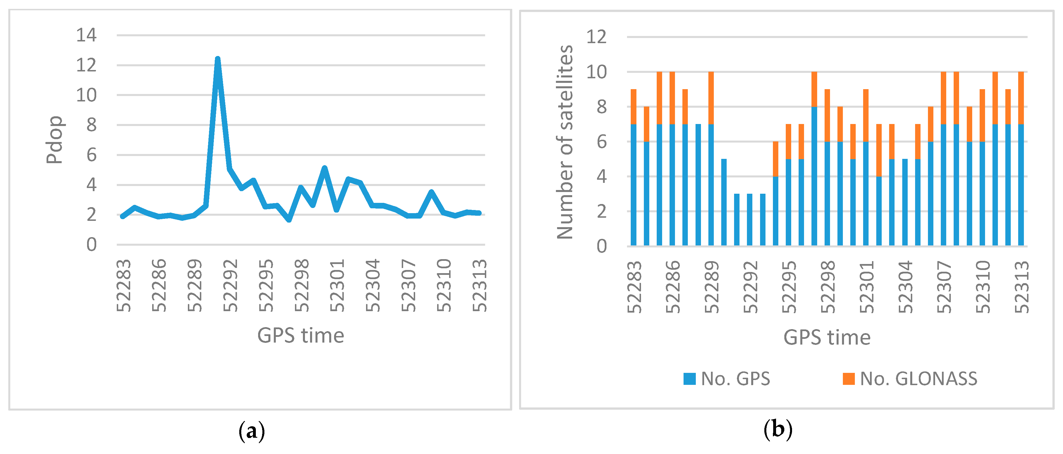
The Applanix APX-15 UAV [38] system was used to capture GNSS and IMU data. Position and orientation were post processed with Applanix POSPAC UAV v7.2. The algorithm used an inertial aided differential GNSS technique [39] with a baseline length up to 30.5 km. The GNSS reference station was obtained from the Norwegian Mapping Authority. Figure 2a shows how the position dilution of precision (Pdop) varied during data capture. The average estimated root mean squared error (RMSE) for the position in the horizontal direction was 0.22 m and 0.32 m in the vertical direction. The estimated RMSE for the orientation in roll and pitch was 0.06 degrees, and 1.30 degrees in heading. Some studies have shown that the GNSS solution can be improved by using the digital elevation model obtained from high-resolution ALS data. The techniques are often referred to as terrain aided GNSS [40], but was not tested in this study.
The estimated positions were transformed to the coordinate system called EUREF89 Norwegian Transversal Mercator projection, which has a mapping scale value close to 1. The same coordinate system was applied for the ALS data. All other processing was performed using Matlab [41].
3. Data Processing and Analysis
3.1. Processing Method
The data processing was divided into nine different processing steps, which can be seen in Scheme 1.
The first step in this processing method was to calculate position and orientation of the laser scanner, described in Section 2.3. The second step was to apply the post processed position and orientation to the laser measurement. The laser points were realized in a local coordinate system. The position and orientation together with the installation calibration parameters provided the information to transform the laser points from this local coordinate system into the global coordinate system described in Section 2.3.
3.2. Point Group Classification
Step number 3 in Scheme 1 starts a classification process. Figure 3 shows the laser points from one scan rotation before the classification were performed. All laser measurements were classified into “groups of tree stem points,” “groups of ground points,” and “not classified points” based on a distance increment analysis for each of the 16 laser beams, also called laser channels. This is a sort of spike landmark extraction, where we searched for points that stands out from the rest [42]. The technique is often used in leg detecting algorithms in robotics [43], but it was also used for tree classification by Forsman et al. [33]. In this method, all laser points were separated into different point groups where each laser channel was treated separately. Two neighboring points were placed into the same point group if the difference between the measured distances was below a given threshold. Based on the evaluation of the field data, the following classification parameters were used:
- Distance measurement increment threshold was set to 0.1 m;
- Maximum tree diameter was set to 0.5 m;
- Trees were assumed to be vertical.
Based on these three classification parameters, all measurements were automatically classified into the three mentioned classes. No manual editing of the point classification was performed.
A point group was classified as a potential group of tree stem points if the distance increment was less than 0.1 m within one laser channel (see Figure 4a). In addition, the horizontal distance between the first and last point in the group had to be smaller than the maximum tree diameter. The analysis was done individually for each of the 16 laser channels. For each point group, a center point and tree radius were estimated using a circle fit algorithm [44]. It is necessary to have three measurements to be able to estimate a center point of the tree stem and a tree diameter. Based on the construction of the laser scanner we can estimate the theoretical maximum distance for a tree detection. Due to the precision and beam divergence, the minimum detectable tree diameter is set to 4 cm. The minimum detectable tree diameter (Minstem) depends on the distance to the scanner, and can be estimated with
The tree stems were assumed to be vertical and well defined, i.e., clearly visible from the scanner and not hidden behind obstacles such as branches and other trees. The tree stem center points established from the different laser channels were subsequently merged together. The vertical distance between each laser channel is two degrees and this was used to decide if two center points belonged to the same tree. To be classified as a tree, there must be five consecutive center points with a vertical distance of two degrees (see Figure 4b). The minimum free visible tree stem (Sstem) of a tree stem can be estimated as
A group of points was classified as ground if the distance increment was smaller than 0.1 m and the horizontal distance was larger than the maximum tree diameter. Finally, a point group was classified as “not classified” if the distance increment was greater than 0.1 m or if the distance increment was below 0.1 m for less than three consecutive measurements.
3.3. Processing Method, Position, and Orientation Improvement
The post processed position and orientation solution described in Section 2.3 had a degraded result due to unfavorable conditions for reception of satellite signals. The proposed method is not very sensitive to position and orientation accuracy, but if the distances between the trees become small, tree identification might become unsuccessful. To avoid unsuccessful identification, it was decided to test scan matching. A version of the iterative closest point algorithm (ICP) called iteratively re-weighed least squares [45] was implemented by adding a Matlab function created by Bergström [46]. In the processing, the robust Welsch criterion function was used. The function estimates a three-dimension translation and rotation between two different point clouds. The first point cloud was locked and called model points. The other point cloud was fitted to the model points and called data points. For each scan rotation, a point cloud was created and a translation and rotation was estimated between the model points and the new data points. It was found that the ICP became more robust if just the estimated tree center points calculated for each scan rotation were entered. Since the amount of estimated tree center points was limited, we allowed the model points to be built up sequentially. After the new data points were transformed to fit the model points, the new transformed data points were added to the model points. In the end, the model points contained all estimated center points. The process is referred to as step 4 in Scheme 1.
3.4. Processing Method, Height Adjustment
To estimate DBH, the heights obtained from the scanner were adjusted. Due to the properties of the scanner and the acquisition, ground points were not present in the entire area for each scan rotation. The ground points from the ALS data were therefore utilized when calculating each center points height above ground and the conversion of the estimated diameter to DBH. The method involves three different height adjustments and was performed separately for each scan rotation. The estimated position accuracy was assumed to be sufficient in the horizontal direction to correspond to the ALS data. The method is further described below.
3.4.1. Height Adjustment Due to Poor 268 GNSS Conditions
Due to the poor GNSS conditions under tree canopies, the TLS data were not accurately aligned in height with the ALS data. The points classified as “ground” from the ALS acquisition were therefore used to estimate a height offset between the ALS and TLS data. This operation is referred to as step 5 in Scheme 1. Since the Velodyne laser scanner has a vertical field of view of 30 degrees, some laser channels were pointing down and others were pointing more upwards. In Figure 5, it is shown that the laser channels pointing down had a higher reliability when estimating the height difference between the ALS ground and the terrestrial ground points. Based on the findings in Figure 5, the laser channels 0, 2, and 4 having vertical observation angles corresponding to −15, −13, and −11 degrees, respectively, in the laser scanner frame system were used in the height difference estimation.
All estimated tree stem center points were adjusted for the estimated height difference between the TLS and ALS data.
3.4.2. Conversion into Height above Ground
After the height adjustment due to poor GNSS observations, the TLS data refer to the same coordinate and height system as the ALS point cloud. Normalized heights (height above ground) for the TLS data were then computed for all TLS points by subtracted their respective ALS TIN heights at the corresponding x and y coordinates, referred to as step 6 in Scheme 1.
3.4.3. Conversion of Estimated Tree Stem Diameters to Tree Stem Diameters at Breast Height
Most of the TLS points were obtained in the region from ground to 3 m above ground. To extract the diameter at breast height, a simple model that assumed that the stem diameter was reduced by 1 cm per m along the stem was used. This is referred to as step 7 in Scheme 1. Points obtained between 0 to 0.5 m were excluded from the processing due to the irregular taper of the lower stem section.
3.5. Clustering of Center Points
In step 8 in Scheme 1, the tree stem center points were clustered based on location and distance analysis. All points closer than 0.3 m to each other were clustered together into one center point group. Each center point group represents a tree with a unique identification. In step 9, the average tree stem diameter and position for each center point group was calculated.
3.6. Evaluation
Finally, the estimated tree coordinates and DBH were compared to the corresponding field reference measurements. Based on these results, mean differences, RMSE, and RMSE% were calculated as
and
where is the estimate, the reference, is the mean reference value, and the number of observations. The tree positon accuracy was evaluated using Equations (3) and (4).
4. Results
The proposed method was able to detect 14 of the 18 trees on the 250 m2 plot. The actual data capture time consumption was 30 s, which did not include the startup time, shutdown time, and the walk in and out of the forest to reach the sample plot. Startup and shutdown can be done while walking to the area of interest. The actual walking path during data capture is shown in Figure 6a. A total of 9.5 million points were measured and 0.2 million of these were automatically classified as tree stems. Based on these points, 3249 center points with a corresponding diameter were estimated. The result is shown in Figure 6b. The center points were clustered to center point group based on location and given a unique tree identification.
Table 2 summarizes the result of the tree stem diameter estimation. The difference between the field measured DBH and the estimated DBH varied between −1 cm and 3 cm for the detected trees. The undetected trees were all small, with a field measured DBH <10 cm, which was smaller than the minimum detectable tree diameter except for one of the four undetected trees. The minimum detectable tree diameter depends on the distance from the scanner to the tree, and is given for each tree in the rightmost column in Table 2. Figure 7 summarizes this minimum detectable tree stem diameter versus distance from the scanner to the tree. For example, if the scan rate is 20, the maximum distance to allow tree detection of a tree with 10 cm in diameter is 7 m.
In Scheme 1, step 9, an average DBH was calculated for each center point group. This was used as the estimated DBH for each detected tree and was compared to the field reference DBH. The result is presented in Table 2 and was used to estimate the mean difference, RMSE, and RMSE%. The estimation was based on Equations (3) to (5). Table 3 summarize these findings. The mean difference between the field reference DBH and the estimated DBH was 0.9 cm, with an RMSE of 1.5 cm.
An average position was calculated for each center point group. Equations (3) and (4) were then used to calculate the mean difference and RMSE. The result is summarized in Table 4.
5. Discussion
The results showed that small trees were difficult to extract with the proposed method. The main reason was that three measurements were required to be able to calculate the tree stem center point and diameter. Based on Equation (1), it is possible to estimate the minimum tree stem diameter observed from different distances. Figure 7 summarizes this minimum detectable tree stem diameter versus distance from the laser scanner to the tree.
In the practical test, there were four trees that were not detected (Table 2). For each of the non-detected trees, the maximum detectable distance was calculated and for three of the four trees, the observed distance was too large for the tree to be detected. The smaller trees would be detected if observed distance or the scan rate had been reduced (Figure 7). If the scan rate is reduced from 20 Hz to 10 Hz, the possible detectable tree diameter is reduced with the same ratio, which means that 17 of 18 trees should theoretically be detectable by reducing the scan rate to 10 Hz. For the tree with ID number 6, the possible detectable tree diameter was smaller than the actual diameter of the tree. This means that one should have expected a positive detection. The actual reason for this was not found, but branches or other vegetation blocking the visibility of the stem might be one explanation.
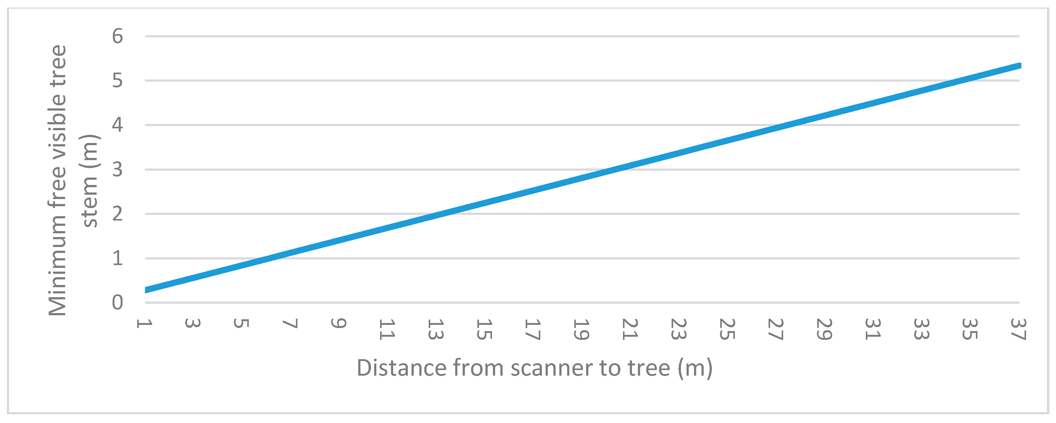
The classification algorithm requires five continuous center points along the stem to be classified as a potential tree. The main reason for this is to filter out points that were falsely classified as a tree stem. Figure 8 shows the relationship between observed distance and the required minimum free visible tree stem. The calculation is based on Equation (2). This requirement was not a big problem in the test area, but different forest conditions with respect to tree species and ages might give other results.
The position and orientation solution in this study were relative good, but not good enough to merge the different scan rotations into one common point cloud. The main reason for this was the poor conditions for GNSS signal reception under the tree canopy.
For many forest inventory applications, the tree position accuracy achieved in this study is sufficient. It is, however, possible to improve the accuracy of the positions. The positions can be improved by different methods:
- Take actions to improve the GNSS accuracy, such as reduce the distance to the GNSS reference station;
- Use the ALS point cloud to extract the tree positions and perform matching per scan rotation to estimate a 2-dimensional translation and rotation for each scan rotation (c.f. Hauglin et al. [47]);
- Develop the proposed method into a three-dimensional SLAM system;
- The trees are assumed to grow vertically. In cases with low orientation accuracy, the trees can be used to estimate an average initial roll and pitch angle.
In the study presented by Bauwens et al. [32], three different tests were performed. The study area was located in Belgium and consisted of 10 different locations. The locations were chosen to maximize the variation in forest types, tree density, and terrain slope. One test was called FARO1 where the reference field was measured from one location with a Faro focus 3D 120. Another test called FARO5 was performed by measuring with the same instrument from five different locations. Finally, a test called ZEB1 was performed by collecting data with a handheld scanner (ZEB1). In terms of accuracy, the result achieved in the current study was between the FARO1 and the FARO5 tests (Table 5).
An important factor when collecting data in the field is time consumption. The method with the smallest time consumption achieved by Bauwens et al. [32] was the FARO1 method, which required 10 min of field work. The required time only included the acquisition of data to get the measurements into a local coordinate system. In the current study, the TLS acquisition took 30 s. The latter also included the acquisition of GNSS and IMU data, which enabled us to produce tree positions in a global reference system. To be able to use the data in operational forest inventory, it is necessary to have the measurements in the same global coordinate system as the ALS data. It is, however, difficult to compare the methods directly because the forest conditions were different with respect to forest type, tree density, terrain conditions, and field plot size. In the current study, we used a plot with a radius of 8.9 m while Bauwens et al. [32] used a radius of 15 m.
6. Conclusions
GNSS signal reception conditions are typically degraded under forest canopies, and the proposed method worked with a relatively coarse positioning and orientation solution. This was possible because the laser measurements were divided into limited time frames determined by the scan rotation. For each scan rotation, tree center points and diameters were calculated. This provided a means to circumvent the need for a high accuracy position and orientation of the moving scanner platform. To avoid the different trees from being mixed, the estimated center points were treated by an ICP algorithm to improve the homogeneity in the merged dataset. This process improved the tree identification process and made the entire process more robust. Future work should be devoted to improving the position and orientation solution with different GNSS techniques, different scan matching technics, or SLAM. Although the method proposed in the current study is in an initial phase of development, it has the potential to become a robust method, rapid and cost-effective acquisition of forest field plot data.
Author Contributions
Ivar Oveland wrote the paper, performed the Velodyne fieldwork, conducted the hardware installation, method development, and processed the data. Marius Hauglin co-authored the paper, prepared the field, and prepared the ALS data. Terje Gobakken planned the ALS acquisition and revised the paper. Erik Næsset and Ivar Maalen-Johansen supervised the study and revised the paper.
Conflicts of Interest
The authors declare no conflict of interest.
References
- Vauhkonen, J.; Maltamo, M.; McRoberts, R.E.; Næsset, E. Introduction to forestry applications of airborne laser scanning. In Forestry Applications of Airborne Laser Scanning; Springer: Berlin/Heidelberg, Germany, 2014; pp. 1–16. [Google Scholar]
- Næsset, E. Predicting forest stand characteristics with airborne scanning laser using a practical two-stage procedure and field data. Remote Sens. Environ. 2002, 80, 88–99. [Google Scholar] [CrossRef]
- Liang, X.; Kankare, V.; Hyyppä, J.; Wang, Y.; Kukko, A.; Haggrén, H.; Yu, X.; Kaartinen, H.; Jaakkola, A.; Guan, F.; et al. Terrestrial laser scanning in forest inventories. ISPRS J. Photogramm. Remote Sens. 2016, 115, 63–77. [Google Scholar] [CrossRef]
- Bayer, D.; Seifert, S.; Pretzsch, H. Structural crown properties of Norway spruce (Picea abies [L.] Karst.) and European beech (Fagus sylvatica [L.]) in mixed versus pure stands revealed by terrestrial laser scanning. Trees 2013, 27, 1035–1047. [Google Scholar] [CrossRef]
- Côté, J.-F.; Fournier, R.A.; Egli, R. An architectural model of trees to estimate forest structural attributes using terrestrial LiDAR. Environ. Model. Softw. 2011, 26, 761–777. [Google Scholar] [CrossRef]
- Hauglin, M.; Astrup, R.; Gobakken, T.; Næsset, E. Estimating single-tree branch biomass of Norway spruce with terrestrial laser scanning using voxel-based and crown dimension features. Scand. J. For. Res. 2013, 28, 456–469. [Google Scholar] [CrossRef]
- Hosoi, F.; Nakai, Y.; Omasa, K. 3-D voxel-based solid modeling of a broad-leaved tree for accurate volume estimation using portable scanning lidar. ISPRS J. Photogramm. Remote Sens. 2013, 82, 41–48. [Google Scholar] [CrossRef]
- Kankare, V.; Holopainen, M.; Vastaranta, M.; Puttonen, E.; Yu, X.; Hyyppä, J.; Vaaja, M.; Hyyppä, H.; Alho, P. Individual tree biomass estimation using terrestrial laser scanning. ISPRS J. Photogramm. Remote Sens. 2013, 75, 64–75. [Google Scholar] [CrossRef]
- Yang, X.; Strahler, A.H.; Schaaf, C.B.; Jupp, D.L.B.; Yao, T.; Zhao, F.; Wang, Z.; Culvenor, D.S.; Newnham, G.J.; Lovell, J.L.; et al. Three-dimensional forest reconstruction and structural parameter retrievals using a terrestrial full-waveform lidar instrument (Echidna®). Remote Sens. Environ. 2013, 135, 36–51. [Google Scholar] [CrossRef]
- Bienert, A.; Scheller, S.; Keane, E.; Mohan, F.; Nugent, C. Tree Detection and Diameter Estimations by Analysis of Forest Terrestrial Laser Scanner Point Clouds. In Proceedings of the ISPRS Workshop on Laser Scanning 2007 and Silvilaser 2007, Espoo, Finland, 12–14 September 2007; pp. 50–55. [Google Scholar]
- Hopkinson, C.; Chasmer, L.; Young-Pow, C.; Treitz, P. Assessing forest metrics with a ground-based scanning lidar. Can. J. For. Res. 2004, 34, 573–583. [Google Scholar] [CrossRef]
- Lovell, J.L.; Jupp, D.L.B.; Newnham, G.J.; Culvenor, D.S. Measuring tree stem diameters using intensity profiles from ground-based scanning lidar from a fixed viewpoint. ISPRS J. Photogramm. Remote Sens. 2011, 66, 46–55. [Google Scholar] [CrossRef]
- Moskal, L.M.; Zheng, G. Retrieving Forest Inventory Variables with Terrestrial Laser Scanning (TLS) in Urban Heterogeneous Forest. Remote Sens. 2012, 4, 1–20. [Google Scholar] [CrossRef]
- Simonse, M.; Aschoff, T.; Spiecker, H.; Thies, M. Automatic Determination of Forest Inventory Parameters Using Terrestrial Laserscanning. In Proceedings of the ScandLaser Scientific Workshop on Airborne Laser Scanning of Forests, Umeå, Sweden, 3–4 September 2003. [Google Scholar]
- Yao, T.; Yang, X.; Zhao, F.; Wang, Z.; Zhang, Q.; Jupp, D.; Lovell, J.; Culvenor, D.; Newnham, G.; Ni-Meister, W.; et al. Measuring forest structure and biomass in New England forest stands using Echidna ground-based lidar. Remote Sens. Environ. 2011, 115, 2965–2974. [Google Scholar] [CrossRef]
- Gorte, B.; Pfeifer, N. Structuring laser-scanned trees using 3d mathematical morphology. Int. Arch. Photogramm. Remote Sens. 2004, 35, 929–933. [Google Scholar]
- Lefsky, M.; McHale, M.R. Volume estimates of trees with complex architecture from terrestrial laser scanning. J. Appl. Remote Sens. 2008, 2, 023521. [Google Scholar]
- Pfeifer, N.; Gorte, B.; Winterhalder, D. Automatic Reconstruction of Single Trees from Terrestrial Laser Scanner Data. ISPRS Int. Arch. Photogramm. Remote Sens. Spat. Inf. Sci. 2004, XXXV, 114–119. [Google Scholar]
- Raumonen, P.; Kaasalainen, M.; Åkerblom, M.; Kaasalainen, S.; Kaartinen, H.; Vastaranta, M.; Holopainen, M.; Disney, M.; Lewis, P. Fast Automatic Precision Tree Models from Terrestrial Laser Scanner Data. Remote Sens. 2013, 5, 491–520. [Google Scholar] [CrossRef]
- Yu, X.; Liang, X.; Hyyppa, J.; Kankare, V.; Vastaranta, M.; Holopainen, M. Stem biomass estimation based on stem reconstruction from terrestrial laser scanning point clouds. Remote Sens. Lett. 2013, 4, 344–353. [Google Scholar] [CrossRef]
- Vonderach, C.; Voegtle, T.; Adler, P.; Norra, S. Terrestrial laser scanning for estimating urban tree volume and carbon content. Int. J. Remote Sens. 2012, 33, 6652–6667. [Google Scholar] [CrossRef]
- Andersen, H.-E.; Clarkin, T.; Winterberger, K.; Strunk, J. An Accuracy Assessment of Positions Obtained Using Survey- and Recreational-Grade Global Positioning System Receivers across a Range of Forest Conditions within the Tanana Valley of Interior Alaska. West. J. Appl. For. 2009, 24, 128–136. [Google Scholar]
- Hauglin, M.; Lien, V.; Næsset, E.; Gobakken, T. Geo-referencing forest field plots by co-registration of terrestrial and airborne laser scanning data. Int. J. Remote Sens. 2014, 35, 3135–3149. [Google Scholar] [CrossRef]
- Bienert, A.; Scheller, S.; Keane, E.; Mullooly, G.; Mohan, F. Application of terrestrial laser scanners for the determination of forest inventory parameters. Int. Arch. Photogramm. Remote Sens. Spat. Inf. Sci. 2006, 36, 5. [Google Scholar]
- Brolly, G.; Király, G. Algorithms for stem mapping by means of terrestrial laser scanning. Acta Silv. Lignaria Hung. 2009, 5, 119–130. [Google Scholar]
- Liang, X.; Litkey, P.; Hyyppa, J.; Kaartinen, H.; Vastaranta, M.; Holopainen, M. Automatic Stem Mapping Using Single-Scan Terrestrial Laser Scanning. IEEE Trans. Geosci. Remote Sens. 2012, 50, 661–670. [Google Scholar] [CrossRef]
- Hopkinson, C.; Lovell, J.; Chasmer, L.; Jupp, D.; Kljun, N.; van Gorsel, E. Integrating terrestrial and airborne lidar to calibrate a 3D canopy model of effective leaf area index. Remote Sens. Environ. 2013, 136, 301–314. [Google Scholar] [CrossRef]
- Liang, X.; Litkey, P.; Hyyppä, J.; Kaartinen, H.; Kukko, A.; Holopainen, M. Automatic plot-wise tree location mapping using single-scan terrestrial laser scanning. Photogramm. J. Finl. 2011, 22, 38–48. [Google Scholar]
- Puttonen, E.; Lehtomäki, M.; Kaartinen, H.; Zhu, L.; Kukko, A.; Jaakkola, A. Improved Sampling for Terrestrial and Mobile Laser Scanner Point Cloud Data. Remote Sens. 2013, 5, 1754–1773. [Google Scholar] [CrossRef]
- Trochta, J.; Král, K.; Janík, D.; Adam, D. Arrangement of terrestrial laser scanner positions for area-wide stem mapping of natural forests. Can. J. For. Res. 2013, 43, 355–363. [Google Scholar] [CrossRef]
- Astrup, R.; Ducey, M.J.; Granhus, A.; Ritter, T.; von Lüpke, N. Approaches for estimating stand-level volume using terrestrial laser scanning in a single-scan mode. Can. J. For. Res. 2014, 44, 666–676. [Google Scholar] [CrossRef]
- Bauwens, S.; Bartholomeus, H.; Calders, K.; Lejeune, P. Forest Inventory with Terrestrial LiDAR: A Comparison of Static and Hand-Held Mobile Laser Scanning. Forests 2016, 7, 127. [Google Scholar] [CrossRef]
- Forsman, M.; Holmgren, J.; Olofsson, K. Tree Stem Diameter Estimation from Mobile Laser Scanning Using Line-Wise Intensity-Based Clustering. Forests 2016, 7, 206. [Google Scholar] [CrossRef]
- Ryding, J.; Williams, E.; Smith, M.; Eichhorn, M. Assessing Handheld Mobile Laser Scanners for Forest Surveys. Remote Sens. 2015, 7, 1095–1111. [Google Scholar] [CrossRef]
- Terrasolid. TerraScan User’s Guide; Terrasolid Ltd.: Helsinki, Finland, 2011. [Google Scholar]
- Kraus, K.; Pfeifer, N. Determination of terrain models in wooded areas with airborne laser scanner data. ISPRS J. Photogramm. Remote Sens. 1998, 53, 193–203. [Google Scholar] [CrossRef]
- Velodyne Lidar, PUCK, VLP16. Available online: http://velodynelidar.com/vlp-16.html (accessed on 8 January 2017).
- Direct Mapping Solutions for UAVs. Available online: http://www.applanix.com/products/dms-uavs.htm (accessed on 8 January 2017).
- Hutton, J.; Bourke, T.; Scherzinger, B.; Hill, R. New Developments of Inertial Navigation Systems at Applanix; Wichmann: Heidelberg, Germany, 2007; pp. 201–213. [Google Scholar]
- Danezis, C.; Gikas, V. An iterative LiDAR DEM-aided algorithm for GNSS positioning in obstructed/rapidly undulating environments. Adv. Space Res. 2013, 52, 865–878. [Google Scholar] [CrossRef]
- MathWorks. Matlab. 2017. Available online: https://se.mathworks.com/ (accessed on 7 February 2017).
- Riisgaard, S.; Blas, M.R. SLAM for Dummies. A Tutorial Approach to Simultaneous Localization and Mapping; BibSonomy: Würzburg, Germany, 2003; p. 126. [Google Scholar]
- Arras, K.O.; Mozos, O.M.; Burgard, W. Using boosted features for the detection of people in 2d range data. In Proceedings of the 2007 IEEE International Conference on Robotics and Automation, Roma, Italy, 10–14 April 2007. [Google Scholar]
- Bucher, I. Circle Fit. 2004. Available online: https://se.mathworks.com/matlabcentral/fileexchange/5557-circle-fit/content/circfit.m (accessed on 15 December 2016).
- Bergström, P.; Edlund, O. Robust registration of point sets using iteratively reweighted least squares. Comput. Optim. Appl. 2014, 58, 543–561. [Google Scholar] [CrossRef]
- Bergström, P. Iterative Closest Point Method. 2016. Available online: https://se.mathworks.com/matlabcentral/fileexchange/12627-iterative-closest-point-method (accessed on 11 March 2016).
- Hauglin, M.; Næsset, E.; Gobakken, T. Assessing the accuracy of co-registered terrestrial and airborne laser scanning data in forests. Proceeding of the ForestSat 2014, Garda, Italy, 4–7 November 2014. [Google Scholar]
Figure 1.
The complete measurement unit with global navigation satellite system (GNSS) antenna, Velodyne VLP16 laser scanner, and the Applanix APX-15 UAV sensor with an inertial measurement unit (IMU) at the bottom. The instrumentation was mounted and carried on a backpack during data capture in the field.

Figure 2.
The position dilution of precision (Pdop) during data capture is shown in (a) and (b) shows the number of satellites in the same time period.
Figure 2.
The position dilution of precision (Pdop) during data capture is shown in (a) and (b) shows the number of satellites in the same time period.
Scheme 1.
Each step in the proposed method is illustrated in the scheme. IPC in step 4 means iterative closest point algorithm, see text in Section 3.3 for details.
Scheme 1.
Each step in the proposed method is illustrated in the scheme. IPC in step 4 means iterative closest point algorithm, see text in Section 3.3 for details.
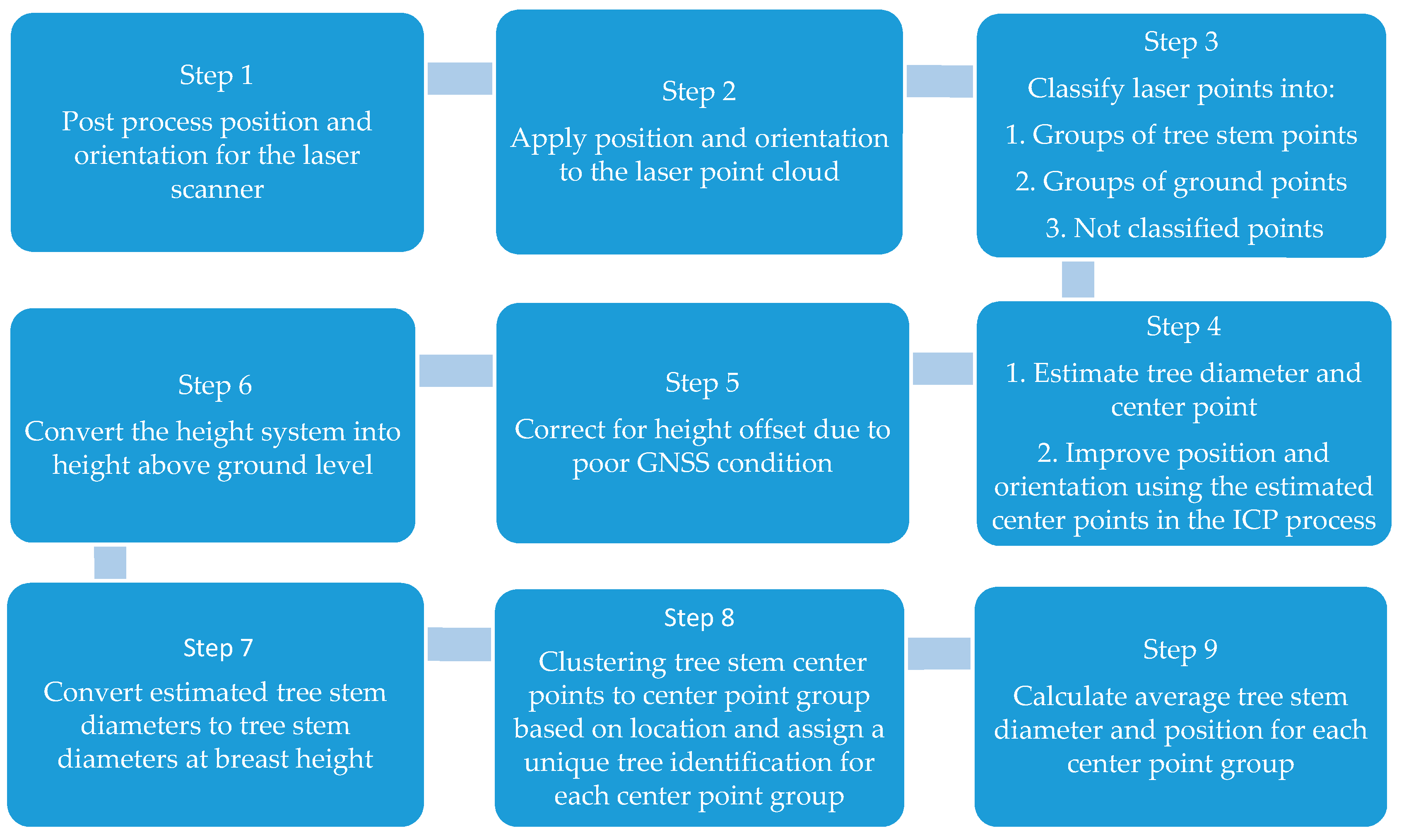
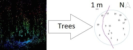
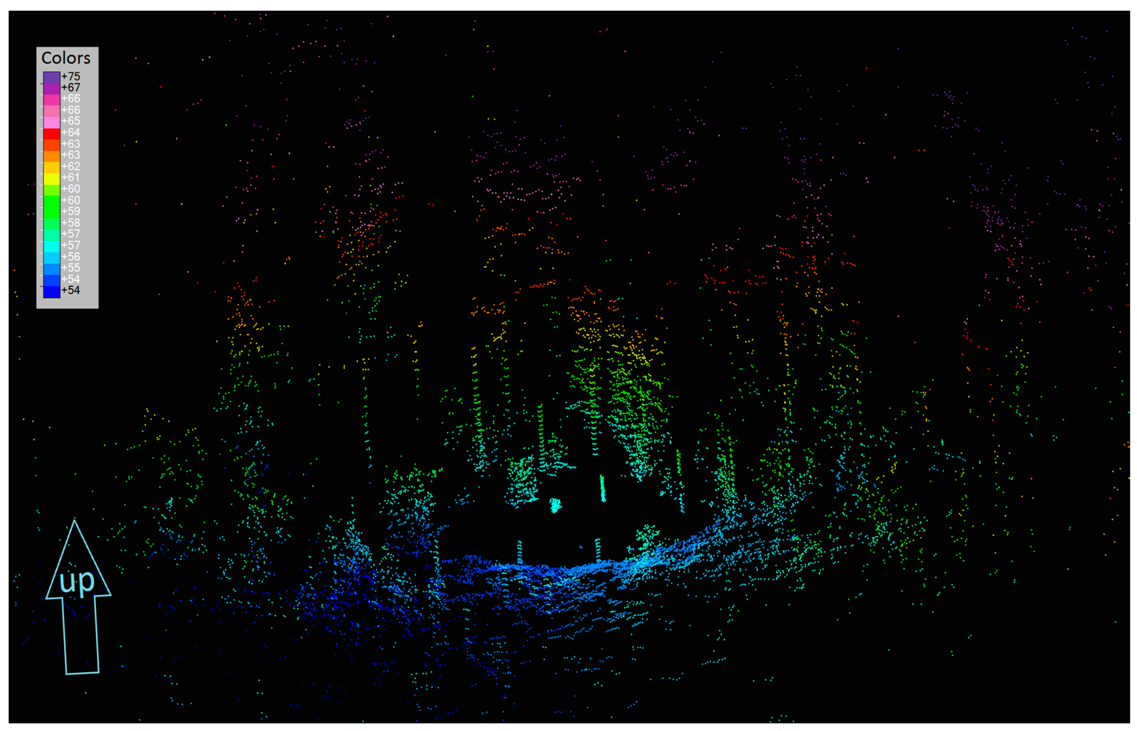
Figure 3.
Approximately 10,000 laser points are collected during one scan rotation. Figure 3 shows an example of one scan rotation from an oblique perspective where the points are colored by elevation. The symmetric vertical structures are tree stems.
Figure 3.
Approximately 10,000 laser points are collected during one scan rotation. Figure 3 shows an example of one scan rotation from an oblique perspective where the points are colored by elevation. The symmetric vertical structures are tree stems.

Figure 4.
Each of the 16 laser channels was treated separately. (a) Illustrates points from the same laser channel reflecting on a tree stem. The red points have all shorter observation distance increment than the given threshold and forming a group of tree stem points. These points are used to estimate a tree stem center point and diameter marked with black color. (b) Illustrates five different groups of tree stem points with the center point marked as a black point and the red points are the laser points. If the number of consecutive tree stem center points were five or more the center points were accepted as a tree and used in step 9 illustrated in Scheme 1.
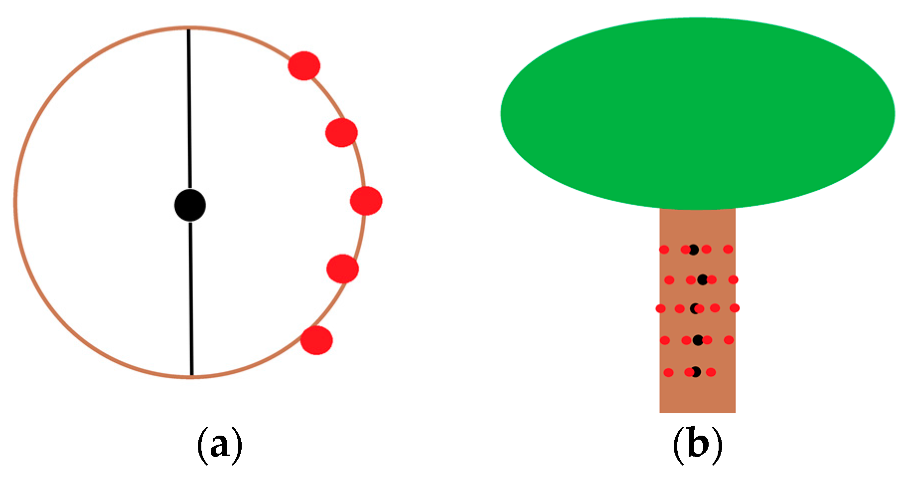
Figure 5.
The height difference between the airborne laser scanning (ALS) ground points and terrestrial laser scanning (TLS) ground points was compared and evaluated based on the 16 different laser channels of the Velodyne laser scanner. The blue bars give the height difference between the ground classified points from TLS data and ground classified points from the ALS data. The orange line tells which laser channels are associated with the corresponding blue bar. The figure shows that laser channels pointing down are more likely to hit the true ground level.
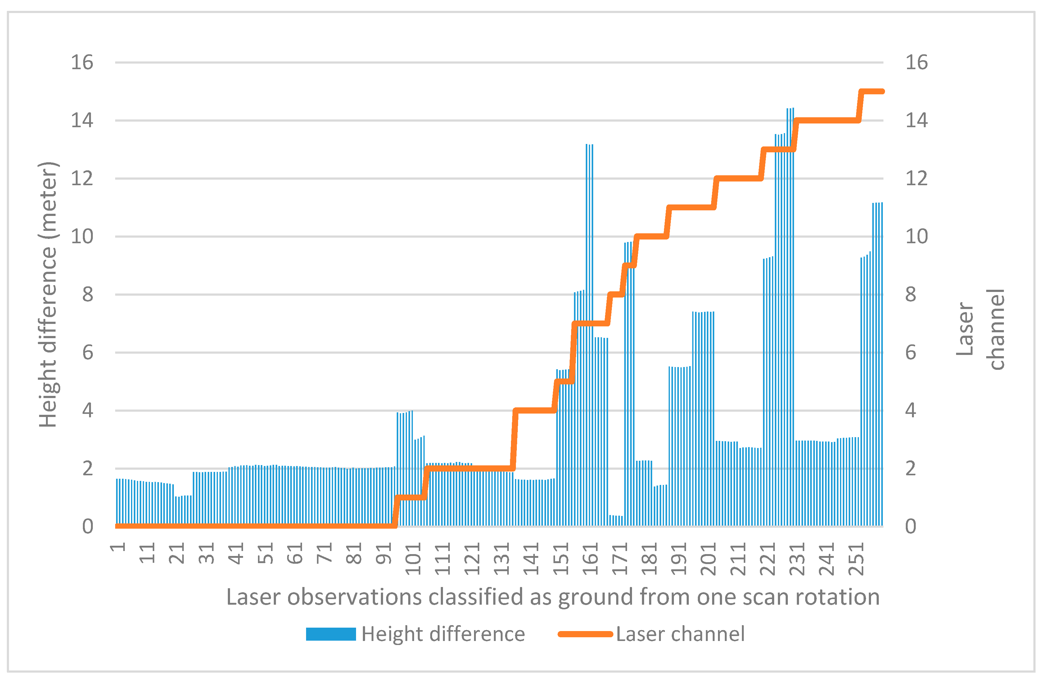
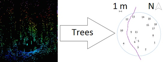
Figure 6.
The walking path (purple line) during data capture and field measured position of the trees are shown in (a). In (b), all estimated center points are shown. Each tree stem center point is colored by a unique color for each tree.
Figure 6.
The walking path (purple line) during data capture and field measured position of the trees are shown in (a). In (b), all estimated center points are shown. Each tree stem center point is colored by a unique color for each tree.
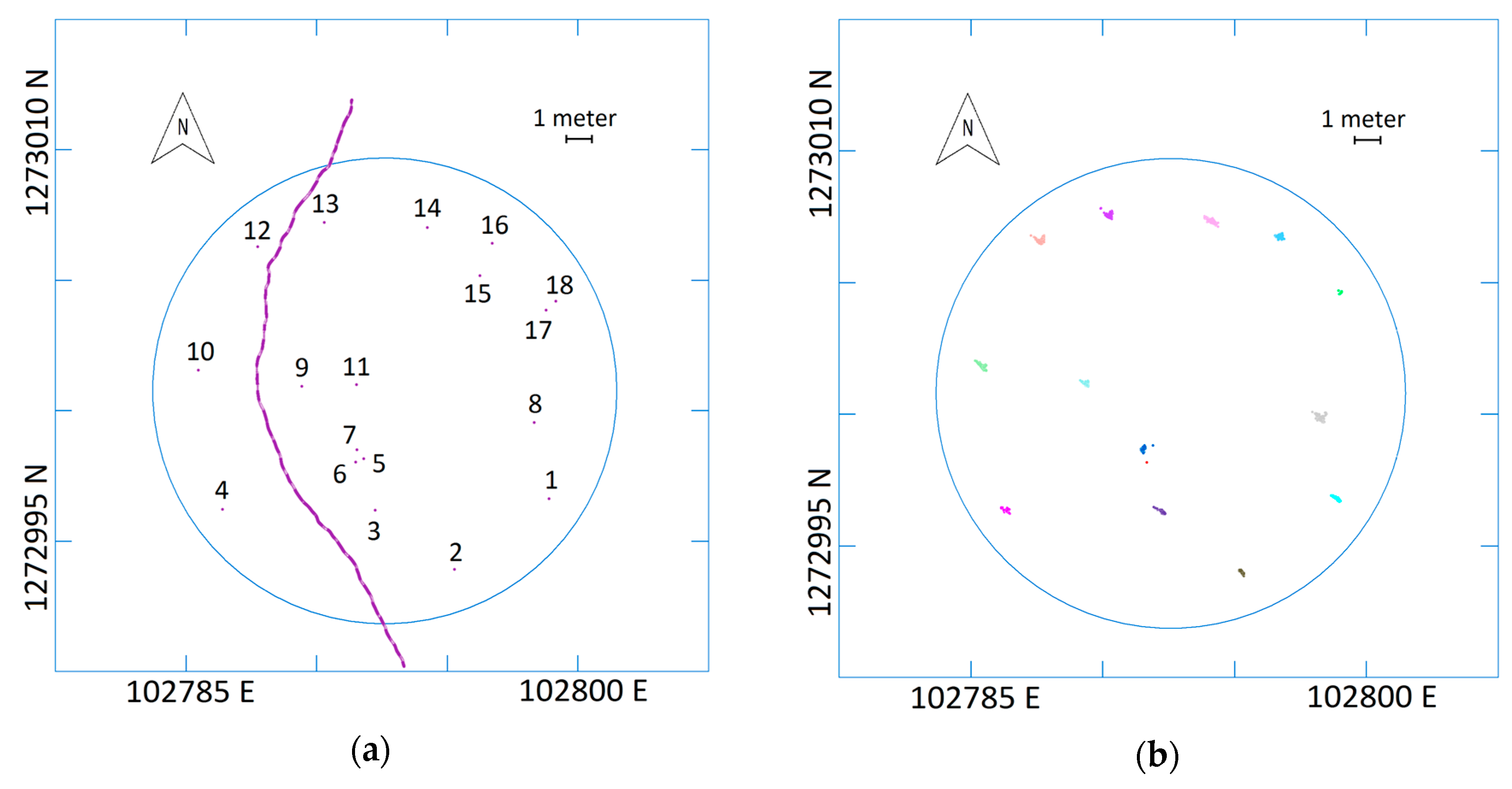
Figure 7.
Minimum diameter at breast height as a function of observation distance and scan rate calculated from Equation (1). Each diameter estimation requires minimum three laser points hitting the tree stem. Then minimum detectable diameter is set to 4 cm.
Figure 7.
Minimum diameter at breast height as a function of observation distance and scan rate calculated from Equation (1). Each diameter estimation requires minimum three laser points hitting the tree stem. Then minimum detectable diameter is set to 4 cm.
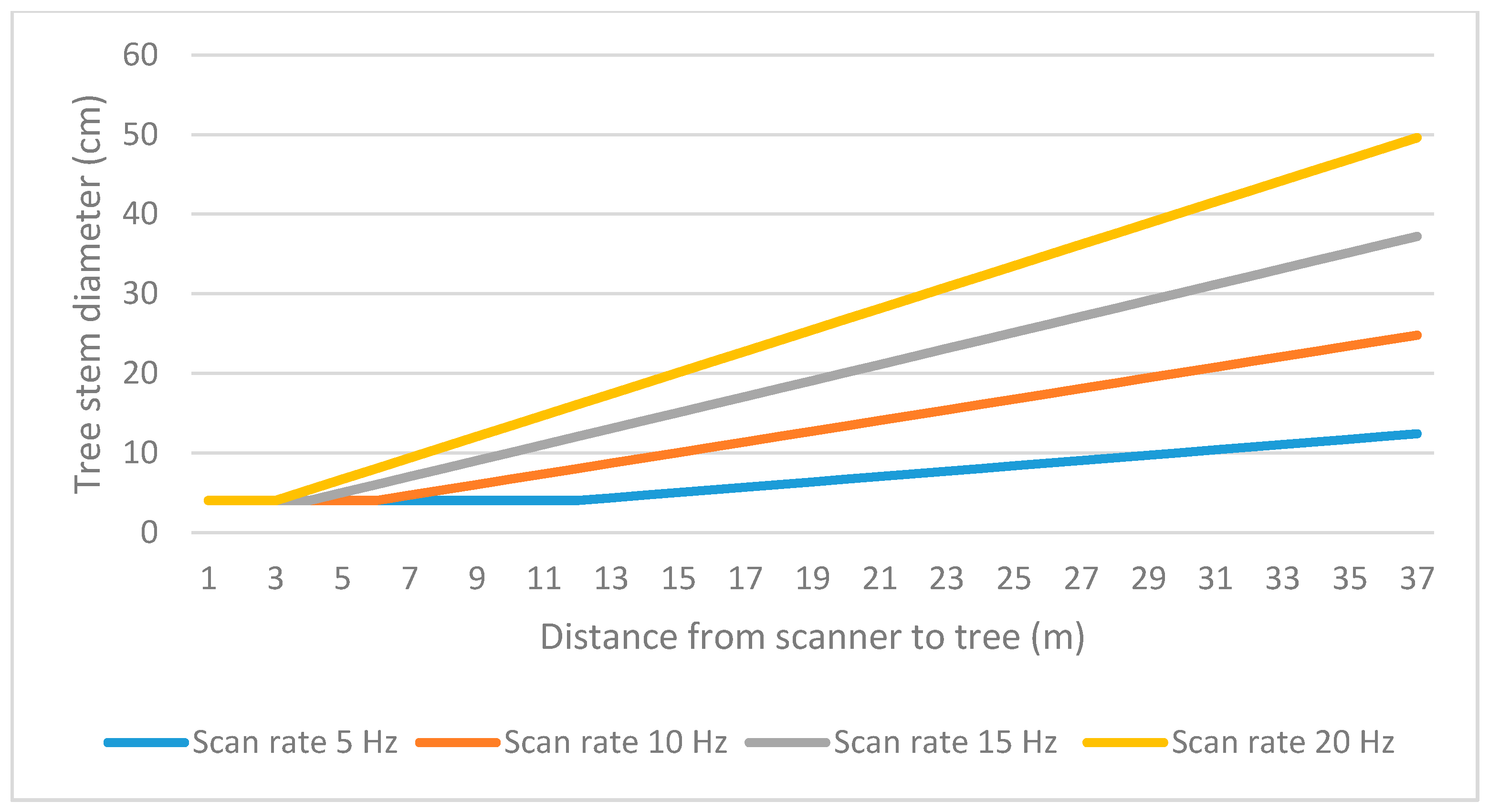
Figure 8.
Calculated minimum unobstructed view to the tree stem based on observed distance. The calculation is based on Equation (2).
Figure 8.
Calculated minimum unobstructed view to the tree stem based on observed distance. The calculation is based on Equation (2).

Table 1.
Summary of tree diameter at breast height (DBH).
| Species | Number of Trees | DBH Min (cm) | DBH Max (cm) | DBH Mean (cm) |
|---|---|---|---|---|
| Pine | 12 | 19 | 39 | 25 |
| Spruce | 6 | 4 | 23 | 9 |
| All | 18 | 4 | 39 | 19 |
Table 2.
Summary at the individual tree level: Estimated DBH, the number of laser points used for detection. The minimum (Min. dist.) and maximum (Max dist.) observed distance to the tree, and field measured DBH. Minimum detectable tree diameter calculated for each tree. All distances are given in cm.
| Tree ID | Estimated DBH | No. of Laser Points | Min. Dist. | Max Dist. | Field Reference DBH | Difference between Field Reference and Estimated DBH | Detect-Able Tree Diameter a |
|---|---|---|---|---|---|---|---|
| 1 | 20.3 | 2800 | 728 | 820 | 20.4 | 0.1 | 10 |
| 2 | 25.3 | 18,628 | 385 | 1630 | 27.2 | 1.9 | 5 |
| 3 | 21.4 | 22,707 | 248 | 630 | 22.6 | 1.2 | 4 |
| 4 | 22.2 | 1850 | 699 | 1190 | 22.5 | 0.3 | 9 |
| 5 | 8.3 | 26 | 240 | 180 | 7.9 | −0.4 | 4 |
| 6 | NIL | 250 | 1140 | 5.6 | 4 | ||
| 7 | 26.0 | 7994 | 574 | 950 | 27.0 | 1.0 | 8 |
| 8 | 23.6 | 5689 | 944 | 1310 | 23.6 | 0.0 | 13 |
| 9 | 19.8 | 29,719 | 398 | 940 | 20.7 | 0.9 | 5 |
| 10 | 19.3 | 20,203 | 651 | 1210 | 21.4 | 2.1 | 9 |
| 11 | NIL | 370 | 9300 | 4.2 | 5 | ||
| 12 | 24.7 | 33,816 | 450 | 1310 | 27.3 | 2.6 | 6 |
| 13 | 17.9 | 33,122 | 364 | 1000 | 19.0 | 1.1 | 5 |
| 14 | 23.8 | 11,624 | 741 | 1050 | 23.5 | −0.3 | 10 |
| 15 | NIL | 720 | 1380 | 5.8 | 10 | ||
| 16 | 26.1 | 9496 | 826 | 1080 | 25.1 | −1.0 | 11 |
| 17 | NIL | 1010 | 1350 | 7.0 | 14 | ||
| 18 | 36.0 | 160 | 1050 | 1160 | 39.0 | 3.0 | 14 |
a Calculated based on the field measured tree positions and the scanner location. See Figure 7 for further details.
Table 3.
Comparison of estimated DBH and field reference DBH. Mean difference and root mean squared error (RMSE).
Table 3.
Comparison of estimated DBH and field reference DBH. Mean difference and root mean squared error (RMSE).
| Number of Trees | Mean Difference (cm) | RMSE (cm) | RMSE% |
|---|---|---|---|
| 14 of 18 | 0.9 | 1.5 | 7.5 |
Table 4.
Comparison of estimated tree positions and field reference positions.
| Number of Trees | Mean Difference (m) | RMSE (m) |
|---|---|---|
| 14 of 18 | 0.21 | 0.23 |
Table 5.
Result for estimated DBH in the current study compared to Bauwens et al. [32].
© 2017 by the authors. Licensee MDPI, Basel, Switzerland. This article is an open access article distributed under the terms and conditions of the Creative Commons Attribution (CC BY) license (http://creativecommons.org/licenses/by/4.0/).
Share and Cite
MDPI and ACS Style
Oveland, I.; Hauglin, M.; Gobakken, T.; Næsset, E.; Maalen-Johansen, I. Automatic Estimation of Tree Position and Stem Diameter Using a Moving Terrestrial Laser Scanner. Remote Sens. 2017, 9, 350. https://doi.org/10.3390/rs9040350
AMA Style
Oveland I, Hauglin M, Gobakken T, Næsset E, Maalen-Johansen I. Automatic Estimation of Tree Position and Stem Diameter Using a Moving Terrestrial Laser Scanner. Remote Sensing. 2017; 9(4):350. https://doi.org/10.3390/rs9040350
Chicago/Turabian StyleOveland, Ivar, Marius Hauglin, Terje Gobakken, Erik Næsset, and Ivar Maalen-Johansen. 2017. "Automatic Estimation of Tree Position and Stem Diameter Using a Moving Terrestrial Laser Scanner" Remote Sensing 9, no. 4: 350. https://doi.org/10.3390/rs9040350
Note that from the first issue of 2016, this journal uses article numbers instead of page numbers. See further details here.