
Segment-before-Detect: Vehicle Detection and Classification through Semantic Segmentation of Aerial Images


1
ONERA, The French Aerospace Lab, F-91761 Palaiseau, France
2
Institut de Recherche en Informatique et Systèmes Aléatoires (IRISA), University Bretagne Sud, UMR 6074, F-56000 Vannes, France
*
Author to whom correspondence should be addressed.
Remote Sens. 2017, 9(4), 368; https://doi.org/10.3390/rs9040368
Submission received: 28 December 2016
/
Revised: 5 April 2017
/
Accepted: 7 April 2017
/
Published: 13 April 2017
(This article belongs to the Special Issue Advances in Object-Based Image Analysis—Linking with Computer Vision and Machine Learning)
Abstract
:Like computer vision before, remote sensing has been radically changed by the introduction of deep learning and, more notably, Convolution Neural Networks. Land cover classification, object detection and scene understanding in aerial images rely more and more on deep networks to achieve new state-of-the-art results. Recent architectures such as Fully Convolutional Networks can even produce pixel level annotations for semantic mapping. In this work, we present a deep-learning based segment-before-detect method for segmentation and subsequent detection and classification of several varieties of wheeled vehicles in high resolution remote sensing images. This allows us to investigate object detection and classification on a complex dataset made up of visually similar classes, and to demonstrate the relevance of such a subclass modeling approach. Especially, we want to show that deep learning is also suitable for object-oriented analysis of Earth Observation data as effective object detection can be obtained as a byproduct of accurate semantic segmentation. First, we train a deep fully convolutional network on the ISPRS Potsdam and the NZAM/ONERA Christchurch datasets and show how the learnt semantic maps can be used to extract precise segmentation of vehicles. Then, we show that those maps are accurate enough to perform vehicle detection by simple connected component extraction. This allows us to study the repartition of vehicles in the city. Finally, we train a Convolutional Neural Network to perform vehicle classification on the VEDAI dataset, and transfer its knowledge to classify the individual vehicle instances that we detected.

1. Introduction
Deep learning for computer vision grows more popular every year, especially thanks to Convolutional Neural Networks (CNN) that are able to learn powerful and expressive descriptors from images for a large range of tasks: classification, segmentation, detection, etc. This ubiquity of CNN in computer vision is now starting to affect remote sensing as well, as they can tackle many tasks such as land use classification or object detection in aerial images. Moreover, new architectures have appeared, derived from Fully Convolutional Networks (FCN) [1], able to output dense pixel-wise annotations and thus able to achieve fine-grained classification. Such architectures have quickly become state-of-the-art for popular datasets such as PASCAL VOC2012 [2] and Microsoft COCO [3]. In an Earth Observation context, these FCN models are now especially appealing, as dense prediction allows us performing semantic mapping without requiring any preprocessing tricks. Therefore, using FCN for Earth Observation means we can shift from superpixel segmentation and region-based classification [4,5,6] to fully supervised semantic segmentation [7].
FCN models have been successfully applied for remote sensing data analysis, notably land cover mapping on urban areas [7,8]. For example, FCN-based models are now the state-of-the-art on the ISPRS Vaihingen Semantic Labeling dataset [9,10]. Therefore, even though remote sensing images do not share the same structure as natural images, traditional computer vision deep networks are able to successfully extract semantics from them, which was already known for deep CNN-based classifiers [11]. This encourages us to investigate further: can we use deep networks to tackle an especially hard remote sensing task, namely object segmentation? Therefore, this work focuses on using deep convolutional models for segmentation and classification of vehicles using optical remote sensing data.
To deal with this problem, we design a three-step pipeline for segmentation, detection and classification of vehicles in aerial images. First, we use the SegNet architecture [12] for semantic labeling on various remote sensing datasets. The predicted map is a pixel-level mask from which we can extract connected components to detect the vehicle instances. Then, using a CNN trained for vehicle classification on the VEDAI dataset [13], we classify each instance to infer the vehicle type and to eliminate false positives. We then show how to exploit this information to provide new knowledge about vehicle types and vehicle localization in the scene.
2. Related Work
This work studies how object-based analysis can be extracted from a dense semantic segmentation in remote sensing data, using deep convolutional neural networks, with an application to vehicles. The idea of using deep networks for classification of remote sensing data is not novel and has been thoroughly investigated in the last few years. For example, Penatti, O.A.B. et al. [11] examined transfer learning from pre-trained convolutional neural networks (CNN) on traditional red-green-blue (RGB) images to remote sensing data. This work has been later consolidated by [6] to better understand CNN-based classification of Earth Observation images. Lagrange, A. et al. [14] used CNN-based superpixel classification to perform semantic segmentation and obtained competitive results on the IEEE GRSS Data Fusion Contest 2015.
However, classification is usually very coarse, even with region-based methods. Dense classification through semantic segmentation has been tackled by the computer vision community with significant improvements thanks to deep learning. Recently, architectures derived from the fully convolutional networks (FCN) [1] obtained state-of-the-art results on datasets such as Pascal Visual Object Classes 2012 (VOC) [2] and Microsoft Common Objects in Context (COCO) [3]. Indeed, the FCN model has been improved to include multi-scale and spatial regularization, e.g., with Conditional Random Fields [15,16]. Although these architectures were introduced for semantic segmentation of multimedia images, usually to discriminate foreground objects versus background, they have also been successfully used for remote sensing data on several datasets [7,17,18,19].
Finally, vehicle detection and vehicle classification are two problems that have been widely investigated in the literature. Studies on vehicle detection in high resolution remote sensing data included histograms of gradients (HOG) with Support Vector Machines (SVM) [20,21], deformable parts models [22], pose estimation using projected 3D models [23], rotationally invariant mixture of models [24] and HOG [25] and multi-scale deep CNN [26]. However, few works investigated both detection and classification. While at the same time introducing the VEDAI dataset, Razakarivony, S. et al. [13] proposed a baseline for detection and classification of vehicles in aerial images using expert features and SVM classifiers. Earlier works include [27] that used a multiresolution segmentation and fuzzy rulesets for classification and [28] that used segmentation and Linear Discriminant Analysis (LDA). Especially, the authors of [28] argue that segmentation before detection helps rule out many false alarms. Our work here follows the same logic, but using deep learning instead of handcrafted features and rules. We try to reconcile semantic segmentation, object detection and fine-grained classification of vehicles using a coarse-to-fine approach. Thus, we go further than bounding box regression, as we want to infer both vehicle shapes and types. We dub our method segment-to-detect, as vehicle detection easily comes as a free byproduct of our semantic segmentation. To the best of our knowledge, our method is the first to apply deep convolutional networks for vehicle segmentation and detection on aerial images. This work extends [29] by providing new insights on band selection when working with multispectral data, thorough analysis of our method on two new datasets for segmentation, detection and classification and the introduction of a re-normalization strategy to improve vehicle classification.
3. Proposed Method
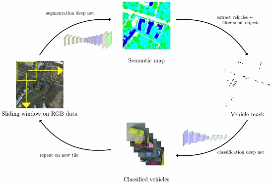
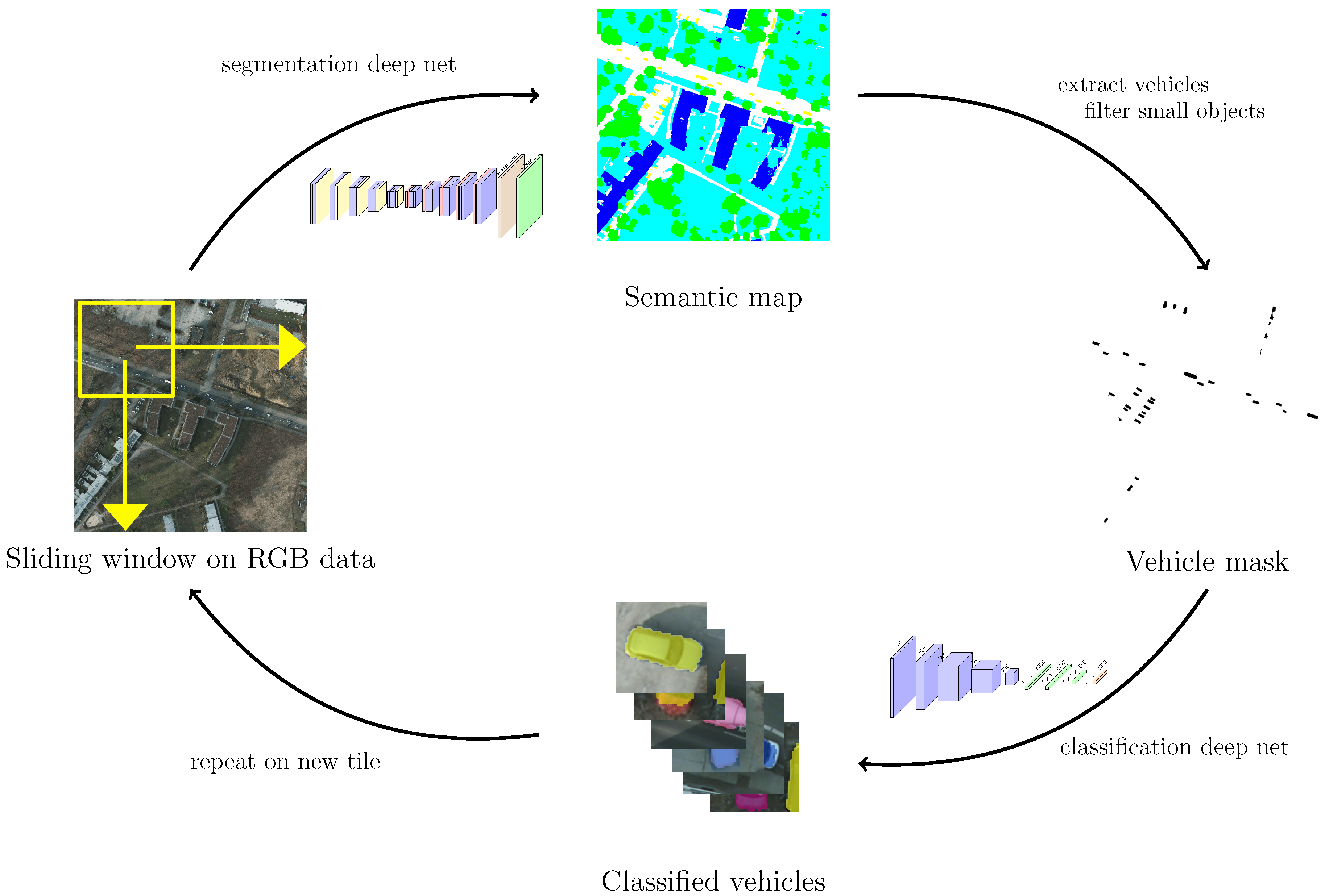
In this work, we introduce a three-step segment-before-detect pipeline to perform vehicle extraction and classification in very high resolution (VHR) remote sensing data over urban areas. Our method consists of three parts, illustrated in Figure 1:
- Semantic segmentation to infer pixel-level class masks using a fully convolutional network;
- Vehicle detection by regressing the bounding boxes of connected components;
- Object-level classification with a traditional convolutional neural network.
In the following sections, we will present how to use fully convolutional neural networks for semantic segmentation and explain how those can be used on VHR remote sensing images. Then, we will briefly present how we regress vehicle bounding boxes from the semantic maps obtained in the first step. Finally, we will present our CNN for individual vehicle classification.
3.1. SegNet for Semantic Segmentation
The computer vision literature abounds with deep network architectures for semantic segmentation. Based on preliminary experimental results, we choose SegNet [12] as our deep network. As illustrated in Figure 2, SegNet has a symetrical encoder-decoder architecture. The encoder is based on the convolutional layers of the VGG-16 model [30]. VGG-16 was designed for the ILSRVC competition and was trained on the ImageNet dataset [31]. Both the encoder and the decoder are made of convolutional blocks, of two or three convolutional layers with a kernel followed by batch normalization [32] and rectified linear units (ReLU). Each block is then sent either into a max pooling layer (encoder) or an unpooling layer (decoder). The maximum pooling operation is used to reduce dimensions and induce translation invariance. The unpooling operation replaces the pooling in the decoder and is the dual operation of the max pooling layer. It relocates the value of the activations into the mask of the maximum values (“argmax”) computed at the pooling stage, which are fed-forward by a skip connection directly into the decoder. Such an upsampling results in a sparse activation map that is then densified by the consecutive decoding convolutions. This allows the network to upsample the feature activations coming out of the decoder up to the original input size, so that the final feature maps have the same dimensions as the input. Therefore, SegNet performs direct pixel-level inference. We argue that, thanks to the precise relocation of abstract features on low level saliency points using the unpooling layers, SegNet is more effective on small objects than deconvolutional counterparts such as DeconvNet [33].
We build our segmentation training set by sliding a px window over each high resolution tile with an overlap of 75% (i.e., a 32 px stride). This overlap acts as data augmentation. For this experiment, we use all the classes from the ground truth. This means that we not only train the model to predict the vehicle mask, but also to assign a label to each pixel according to each class, e.g., “building” or “vehicle”.
At testing time, we process the tiles with a sliding window of px with an overlap of 50% (i.e., a 64 px stride). Overlapping predictions are averaged to smooth predictions along the window edges, thus avoiding a “mosaic” effect.
During training, we initialize SegNet’s encoder using weights of a pre-trained VGG-16 on ImageNet. Following the conclusions of [19], we set the learning rate for the encoder as half the learning rate for the decoder. We train the network with Stochastic Gradient Descent (SGD).
3.2. Small Object Detection
Assuming that we will work on VHR aerial images on which a human observer can distinguish cars, the semantic maps predicted by SegNet should be accurate enough to avoid the merging of neighboring cars into a single blob. If this hypothesis is verified, finding vehicle instances in the pixel-level mask is only a matter of extracting connected components. Then, it is possible to regress the bounding box of the vehicle under the mask.
However, predictions from SegNet can be noisy, as CNN tends to have blurred transitions between classes [34]. Therefore, to alleviate perturbations in the predictions coming out of the network, we first operate morphological opening with a small radius to erode the vehicle mask. Second, we eliminate the objects smaller than a threshold to remove potential false positives due to segmentation artifacts such as vents on roofs or clutter on the street that might have been misclassified as vehicles. Despite its simplicity, this morphological opening, combined with the connected component extraction, is enough to perform efficient vehicle detection.
3.3. CNN-Based Vehicle Classification
Assuming that we have identified a candidate vehicle, the most relevant object-level information that we seek is its type, e.g., if the vehicle is a car, a truck, a van, etc. This is a standard image classification problem that can be addressed by CNN. CNNs are artificial neural networks [35] where convolutions stacked with non-linearities (such as or the rectified linear unit ), also called ReLU) act as learnable feature extractors. Pooling layers are intertwined with the convolutions. Finally, the flattened activations are classified using traditional fully connected layers.
Following common practices [6,36], we will consider a pre-trained CNN on ImageNet [31], and we will fine-tune it on our dataset of aerial images of vehicles. Considering that lots of CNN models of increasing complexity have been proposed over the years, we will compare the most cited ones to better understand how to choose a specific pre-trained network for small object (≃30 × 30) classification in remote sensing data. Especially, we choose to compare LeNet [35], AlexNet [37], and VGG-16 [30].
As our goal is to train our vehicle classifier on a larger dataset and then perform classification on unseen data from a different dataset, we expect to be faced with an overfitting problem. Indeed, we are trying to transfer knowledge from one dataset to another, which is linked to domain adaptation. To increase the generalization power of a classifier, two techniques can be used: data normalization and data augmentation. Data normalization tries to minimize the differences between the training and testing datasets. Data augmentation generates new synthetic images from the original ones to improve the classifier’s robustness.
As a data normalization strategy, we propose to normalize the direction of all vehicles both at training and testing times. At training time, we use the bounding boxes from the annotations to extract the vehicle main direction, and then apply a rotation around the center of the vehicle so that all vehicles have the same principal direction, e.g., horizontal. At testing time, the same will be done but on the inferred vehicle masks extracted from the segmentation results.
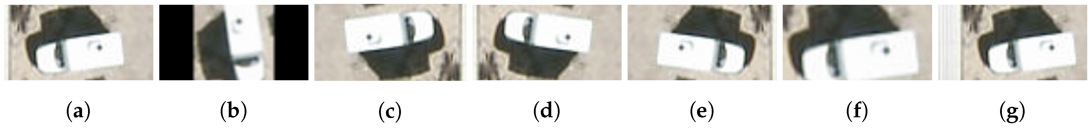
As a data augmentation strategy, we propose to perform geometrical operations in order to increase the network’s resilience to such perturbations. Therefore, for each image, we also include variants with translations ( px), zooms (up-to 1.25x), rotations ( and 270°) and axial symmetries, as illustrated by Figure 3. Only the 180° rotation is used in combination of the data normalization strategy to enforce consistency in the vehicle directions.
4. Experiments
4.1. Datasets
4.1.1. VEDAI
The VEDAI dataset [13] is comprised of 1268 RGB tiles ( px) and the associated infrared (IR) image at 12.5 cm spatial resolution. For each tile, annotations are provided with the vehicle class, the coordinates of center and the four corners of the bounding polygons for all the vehicles in the image. VEDAI is used to train a CNN for vehicle classification. This CNN will then be used to classify the vehicles segmented on the other dataset. Results on this dataset are cross-validated using 2/3 of the images for training and 1/3 for testing.
4.1.2. ISPRS Potsdam
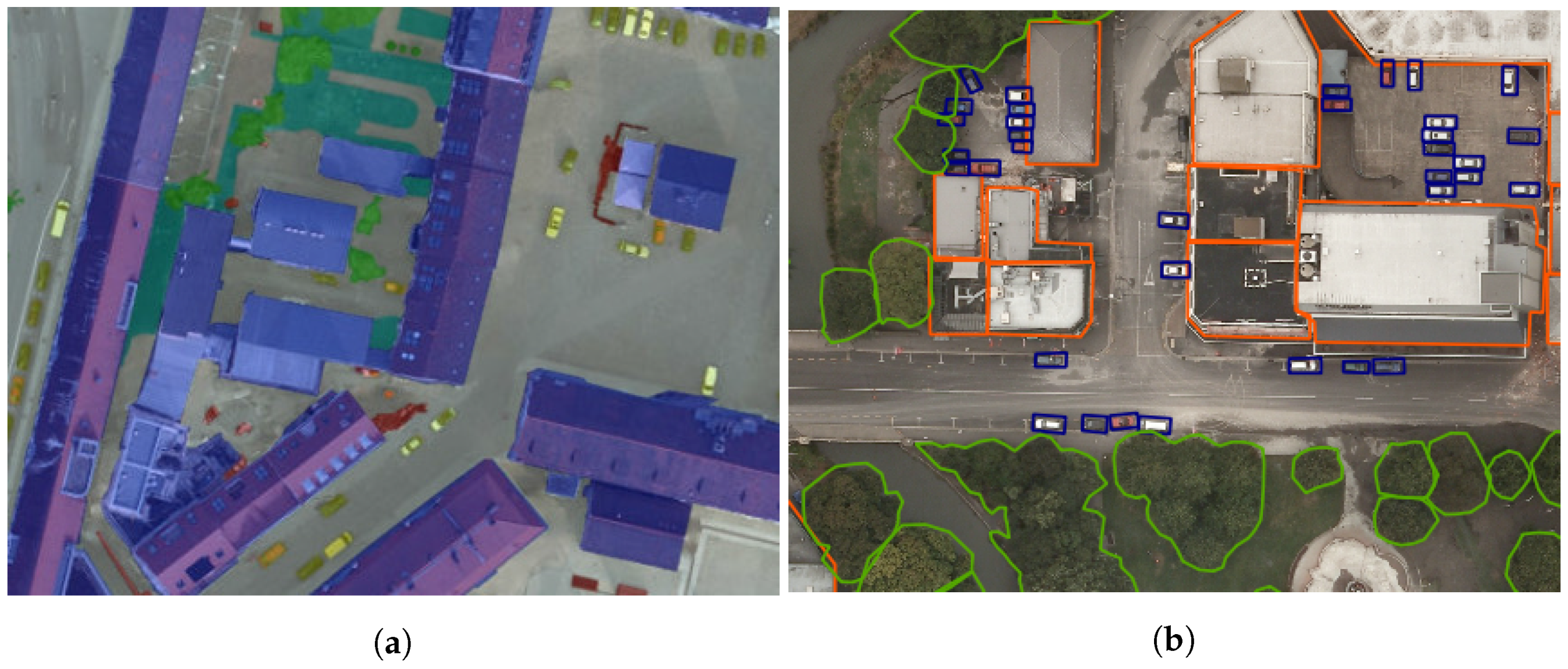
The ISPRS Potsdam Semantic Labeling dataset [9] is comprised of 38 ortho-rectified aerial IRRGB images ( px) at 5 cm spatial resolution, taken over the city of Potsdam (Germany). A comprehensive pixel-level ground truth is provided for 24 tiles, which are the tiles we work on (cf. Figure 4a). We train a SegNet on this dataset and then classify the detected vehicles using the CNN trained on VEDAI. Results on this dataset are cross-validated on a three-fold train/test split (18 tiles for training, six tiles for testing). Resolution is downsampled to 12.5 cm/pixel to match VEDAI.
On this dataset, we manually build an enhanced ground truth by further dividing the “car” class into several subcategories from the VEDAI dataset: “cars”, “vans”, “trucks” and “pick ups”. We discard other vehicles that are present in the optical data, such as construction vehicles, but were labeled as “clutter” in the original ground truth. As illustrated in Table 1, this dataset is dominated by the “car” class (94%).
4.1.3. NZAM/ONERA Christchurch
The Christchurch dataset consists of 10 cm/pixel ortho-rectified aerial red-green-blue (RGB) images captured after the earthquake that struck the town of Christchurch (New Zealand) on 22 February 2011. Four images (≈5000 × 4000 px per image) were annotated by ONERA/DTIS [22] with the following classes: “buildings” (797 objects), “cars” (2357 objects), and “vegetation” (938 objects). All objects are given a polygonal bounding box, which makes these annotations coarser than the dense pixel-level ground truths from the ISPRS Potsdam (cf. Figure 4b).
As for the ISPRS Potsdam dataset, we build an enhanced ground truth by manually annotating trucks, vans and pick-ups. As illustrated in Table 1, this dataset is dominated by the “car” class (94%). We train a SegNet on this dataset and then classify the detected vehicles using the CNN trained on VEDAI. Results are cross-validated on a three-fold train/test split (three tiles for training, one tile for testing). As previously, resolution is downsampled to 12.5 cm/pixel.
4.2. Semantic Segmentation
4.2.1. ISPRS Potsdam
We report in Table 2 the F1 scores and the overall accuracy on our validation set of the ISPRS Potsdam dataset. Theses metrics are computed on an alternative ground truth obtained by eroding the class borders by a disk of radius 3 px, as per the dataset instructions. SegNet trained on the downscaled tiles at 12.5 cm/pixel is able to perform very precise semantic segmentation on all the classes, with an overall accuracy of more than 90% using the RGB images on our validation set. As a comparison, current state-of-the-art on the held-out test set is at 90.3% using both IRRG and the Digital Surface Model (DSM) [17]. Our results are competitive with the 89.7% overall accuracy obtained by [17] using the 5 cm/pixel IRRG information only, including a Conditional Random Field (CRF) regularization (which we do not use). We also report the results obtained by one of our SegNet trained on the IRRG 5 cm/px tiles on a held-out test set, which achieves a 90.0% overall accuracy, which is even better than previous FCN or the ResNet on optical data only (“DST_2” and “CASIA” lines from the leaderboard http://www2.isprs.org/potsdam-2d-semantic-labeling.html). In our case, even using the downscaled 12.5 cm/pixel images, vehicles are especially well segmented with a pixel-wise accuracy of 82.3% and an F1 score on the eroded ground truth at 95.7%, which is promising for the connected component extraction part. The intersection over union score on the dataset for vehicles reaches 82.4%. Processing one tile on the ISPRS Potsdam dataset takes around 60 s using an NVIDIA Tesla K20c. Qualitative results are displayed in the Figure 5.
4.2.2. NZAM/ONERA Christchurch
As the NZAM/ONERA Christchurch dataset only has (possibly overlapping) bounding boxes annotations for vegetation (mostly trees), buildings and vehicles, we have to refine this ground truth into a dense pixel-wise annotation. To do so, we define four classes: “background”, “building”, “vegetation” and “vehicle”. We build the ground truth by first labeling the pixels from the “building” bounding boxes, then “vehicles” and finally “vegetation”. We chose this order as some vehicles are on rooftops and trees can occlude some vehicles. To take into account the uncertainties of the bounding boxes, we set the borders as undefined, e.g., we erode the bounding boxes by 5 px (15 px for the buildings) and we do not learn on those pixels.
As illustrated in Table 3, SegNet trained on NZAM/ONERA Christchurch reaches 61.9% pixel-wise accuracy on the vehicles, which is competitive compared to the ISPRS Potsdam results, considering that the annotations are significantly coarser than the pixel-level ground truth from this dataset. This is especially interesting, as it shows that semantic segmentation is affordable with coarse annotations, even bounding boxes originally designed for detection. Processing one tile on the Christchurch dataset takes around 120 seconds using an NVIDIA Tesla K20c. Qualitative results are displayed in the Figure 5.
4.3. Detection Results
For both datasets, we apply a morphological opening with a radius of 3 px (≃ 35 cm uncertainty in the predicted shapes for the vehicles) to isolate potentially merged cars and we remove isolated components with a surface smaller than 100 px. Then, we perform a connected component extraction and we regress the bounding boxes around each component. For the ISPRS Potsdam dataset, as the ground truth annotations were originally dense pixel labels, we regressed a bounding box for each component, where we manually corrected occasional errors.
Following common practices in object detection [2], we define a true positive as a predicted bounding box for which the intersection over union (IoU) with a bounding box from the ground truth is over 0.5. If there are several predictions for the same vehicle, we keep the one with the highest IoU and consider the other predictions as false positives. For the NZAM/ONERA Christchurch, we tested our method on the same tile as the work from [24], which used a Discriminatively trained Model Mixture (DtMM) comprised of five models, each taking care of one principal orientation in order to be rotationally invariant.
To evaluate the effect of the morphological processing on the instance segmentation problem, we report in Table 4 the mean instance-wise intersection over union (mIoU) and final detection precision/recall for different preprocessing strategies. This shows that, although the direct component extraction achieves a respectable detection accuracy and a 70% instance-level IoU, using a simple morphological opening significantly helps to isolate cars and improves both the detection and the instance-level segmentation by removing many false positives and strongly increasing the precision. This is especially true for the NZAM/ONERA dataset where the coarse annotations result in coarser semantic maps. Moreover, removing small objects further increases the detection accuracy by eliminating classification artifacts, e.g., very small objects wrongly assigned to the “car” class during inference. The full pipeline achieves an instance-level IoU of more than 74% on the ISPRS Potsdam dataset and more than 70% on the NZAM/ONERA dataset.
Finally, we report the various vehicle detection results in Table 5. On NZAM/ONERA Christchurch, our segment-before-detect pipeline performs significantly better than both DtMM and HOG + SVM-based methods. Although no results for vehicle detection on the ISPRS Potsdam exist to the best of our knowledge, we report both precision and recall on this dataset as our method seems to perform very well on these images. Some qualitative visualizations are shown in Figure 6.
Christchurch is a more challenging city for two reasons. First, the vehicle density is higher than for Potsdam, with lots of cars packed in small areas. Second, the coarse annotations amplify the FCN inclination to predict blurred transitions between classes, which results in coarser vehicle masks than for the ISPRS dataset as shown in Figure 5 (the object-level average IoU on Christchurch reaches 66.6%, compared to more than 80% for Potsdam). This combination makes it harder to extract individual vehicles, although our simple morphological opening approach still works well. Thus, even though SegNet performs well on the Christchurch dataset for vehicle segmentation, the classifier has to deal with ill-conditioned bounding boxes, occasionally covering more than one vehicle. We stress out that our deep network was trained using the exact same data that were previously used for object detection, i.e., the bounding boxes. We only refined the ground truth by eroding the borders and removing these uncertain pixels from the training set. Therefore, it is quite interesting to see that using segmentation as a proxy for vehicle detection can be a reasonable approach with better performances than previous complex methods of the state-of-the-art. The connected component extraction bottleneck could later be improved by investigating a more robust bounding box extraction, either by using finer morphological approaches such as watershed segmentation of the distance map [38], or by integrating the instance prediction in the network [39].
4.4. Learning a Vehicle Classifier
For vehicle classification, we compare three CNN architectures of increasing complexity: LeNet [35], AlexNet [37] and VGG-16 [30]. LeNet-5 is a small CNN that will be trained from scratch on our vehicle dataset, with input patches at resolution . AlexNet and VGG-16 are bigger CNN and winner of the ImageNet competition in 2012 and 2014. Preliminary experiments show that the CNN overall accuracy is improved by 10% when using pre-trained weights on the ImageNet dataset, which is consistent with results from [6,11]. Therefore, those CNN will be simply fine-tuned with input patches at resolution and , respectively. Note that the dimensions of the input patches are chosen so that we are able to keep the pre-trained weights of the fully connected layers. However, our true patches will be extracted using the inferred vehicle bounding boxes and therefore will be smaller, as most vehicles are around . Practically, we use patches centered on the vehicle bounding boxes including an additional spatial context of 16 pixels in all directions as this receptive field gave the best results in preliminary experiments. A smaller receptive field decreases accuracy as less contextual cues as provided, while a bigger receptive field can include several vehicles in the same patch. The patches are then upsampled by bilinear interpolation along the largest dimension to match the expected resolution of our CNN, while the smallest dimension is padded with white noise.
All models are trained (or fine-tuned) for 20 epochs, i.e., 20 full passes on the training data from our vehicle dataset using Stochastic Gradient Descent (SGD) and backpropagation using a batch size of 128 for AlexNet and LeNet, 32 for VGG-16 due to memory limitations. We train using the step policy and therefore divide the learning rate by 10 at 75% of the training. When fine-tuning, we retrain the whole network, except for the last layer, which is learnt from scratch and that has a 10 times higher learning rate. We also use dropout [40] in the last fully connected layers to ensure better generalization.
Unsurprisingly, the better the CNN performed on ImageNet, the better it performs on VEDAI, as illustrated in Table 6. However, the most complex network (VGG-16) increases the accuracy only slightly, while strongly slowing down the computations. Bear in mind that our pipeline does not depend on any particular CNN architecture and could be adapted to any other deep network, including the powerful but more memory expensive ResNet [41].
Table 7 details vehicle classification results on VEDAI according to different data preprocessing strategies. Data augmentation by geometrical transformations (denoted “DA”) improves the overall accuracy and increases the overall stability of the predictions, although with a high sensitivity on the “Plane” class. Re-normalization (denoted “R”) also tends to improve the classification results, including the average accuracy, which makes it more robust than data augmentation alone. The combination of the two offers the best results. Therefore, our final results on the ISPRS Potsdam and NZAM/ONERA Christchurch datasets will be obtained using AlexNet and both data augmentation and renormalization strategies.
4.5. Transfer Learning for Vehicle Classification
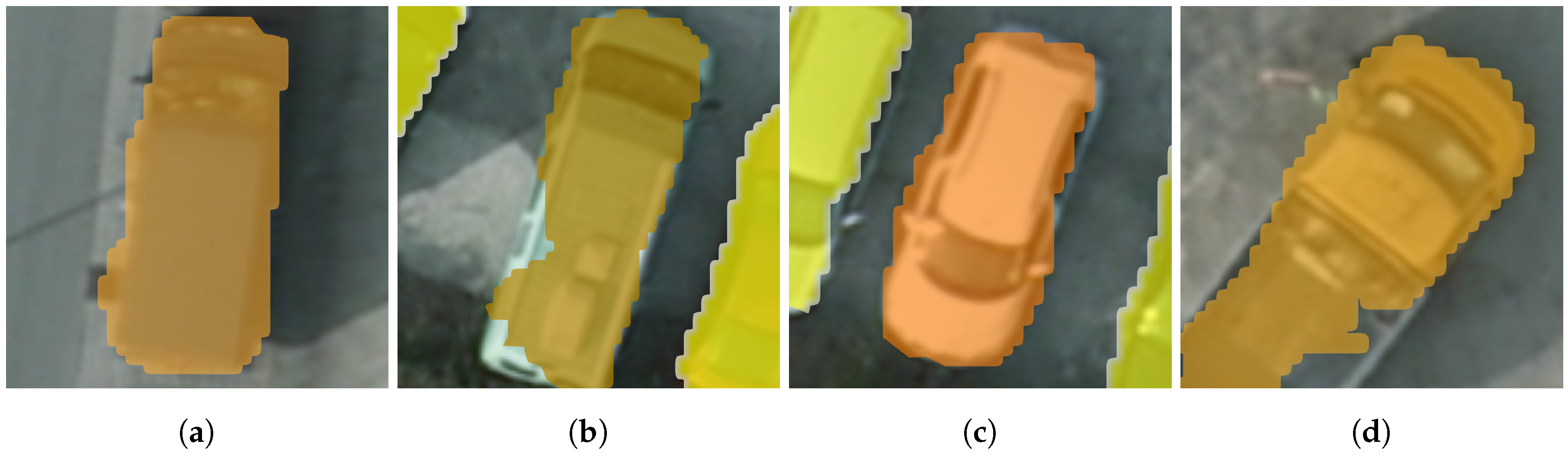
Now that we are able to detect vehicles, we can move onto individual vehicle classification. In Table 8, we report the classification results of our CNN trained on VEDAI and applied on the detected vehicles inferred by SegNet on the ISPRS Potsdam and NZAM/ONERA Christchurch datasets. Results are aggregated on the same three-fold split used to cross-validate the semantic segmentation from Section 4.2. Furthermore, as the initial datasets are heavily dominated by cars compared to the other classes (more than 90%), we also report the metrics for a constant output dummy classifier that would only predict the “car” class. This constant classifier would be correct 94% of the time, but would never predict anything else than cars. This constant classifier already achieves an excellent accuracy; however its average accuracy is of course very bad. This baseline is denoted “Cars only” in the Table 8. The CNN based classifiers manage to extract some meaningful information about the types of vehicles, significantly improving the AA and being competitive in OA. Especially, VGG-16 even manages to be quite effective for the vehicle type classification on the NZAM/ONERA Christchurch dataset. Figure 7 shows some examples of correct segmentation but subsequent misclassification, while Figure 8 illustrates some vehicle instances where our deep network-based segmentation and classification pipeline was successful.
The fact that the average accuracy of the models on Potsdam are lower than results reported on VEDAI might be a consequence of the high statistical sensitivity of the results with respect to the unbalance of the classes. Indeed, each split for the cross-validation only contains ≃15 examples of trucks and pickups. However, the model was trained on the more balanced VEDAI dataset and directly applied on Potsdam. Therefore, the test bias on the prior for cars cannot be stronger than the bias learnt on VEDAI during training. On the contrary, we assume that our networks suffered from overfitting on the vehicle appearance from VEDAI as the datasets use images taken from two similar but subtly different environments using different sensors. Indeed, Potsdam is an urban European city, whereas VEDAI images have been shot over Utah, in a more rural American environment.
To alleviate the difference in sensor calibration, we projected the color scheme from the test image to match the statistics from VEDAI, using the following formula:
where m denotes the mean of pixel values in the dataset, the standard deviation pixel-wise and X the image to be processed. This operation is applied for each channel. However, this is not enough as this only takes care of colorimetry.
Brands and vehicle appearances still matter a lot, as illustrated by the better results in Christchurch, which is a town in New Zealand with cars and pick-ups with an American look. Vehicle brands and different land covers around the cars might influence the classifiers by introducing unforeseen perturbations. This is particularly true for rarer vehicles such as pick-ups and trucks, which significantly differ in the US and Europe.
More comprehensive regularization during fine-tuning and/or training on a more diverse dataset would help alleviate this phenomenon. More generally, the transfer learning issue relates to unsupervised domain adaptation [42], which is still under heavy investigation for remote sensing data, with techniques such as [43]. On a dataset with a larger variety of vehicles than the ISPRS Potsdam and NZAM/ONERA Christchurch, it should be feasible to fine-tune the VEDAI trained CNN to work around this adaptation problem.
4.6. Traffic Density Estimation
Now that we have extracted individual vehicles from the image, the most basic task that we can perform is estimating the number of objects in a designated area. For fair comparison, we subdivide the testing sets for the two datasets into grids (i.e., m2 area) and we compute the relative errors in the vehicle count by comparing the number of vehicles extracted from SegNet’s mask against the ground truth, i.e.:
Averaged results (rounded to the nearest integer) for each dataset are detailed in Table 9. On both ISPRS Potsdam and NZAM/ONERA Christchurch datasets, the vehicle count is less than 10% (predictions are right ±5 vehicles). Christchurch estimations have a higher error, although they might still be accurate enough for a first approximation.
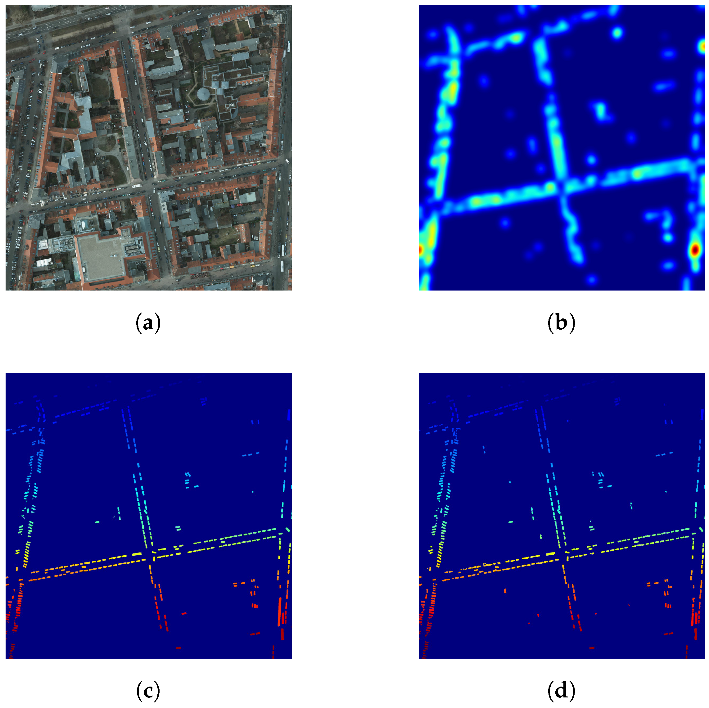
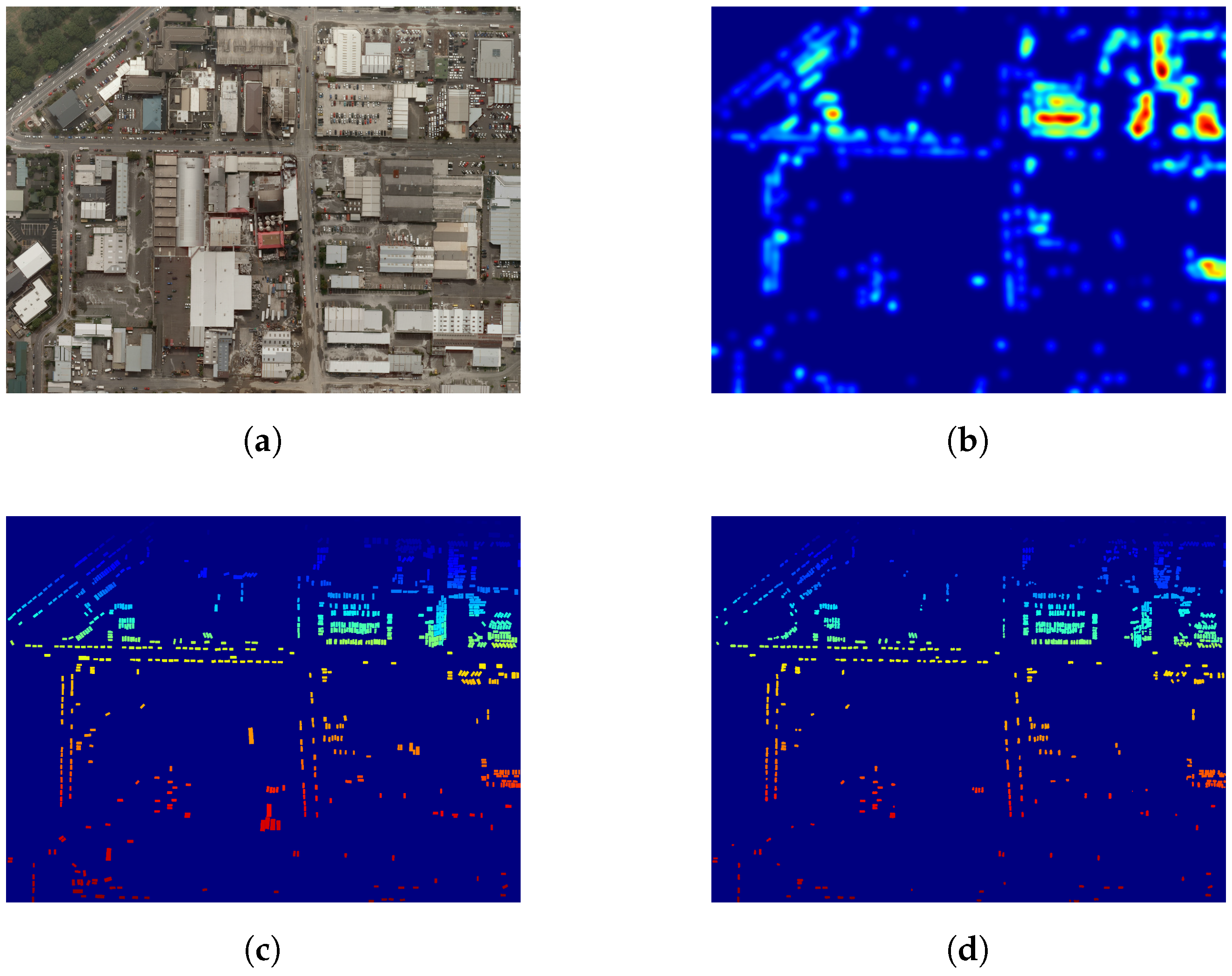
As we also have the spatial location of all the predicted vehicles, we can go further than simple vehicle counting and spatialize this information by computing vehicle density maps across each tile, as illustrated in Figure 9 and Figure 10. This vehicle heat map could then be used with other geo-information systems (GIS), such as OpenStreetMap to automatically find potential parking lots [25], busy roads, etc.
5. Conclusions
In this work, we presented a three-step framework segment-before-detect to segment, detect and classify vehicles from aerial RGB images using deep learning. More precisely, we showed that deep networks designed for semantic segmentation such as SegNet are useful for scene understanding of remote sensing data and can be used to segment even small objects, such as cars and trucks. Moreover, we showed that vehicle detection came without effort from this high resolution segmentation using simple connected component extraction, with results superior to previously used expert methods. We illustrated this fine segmentation on two challenging remote sensing datasets on the cities of Potsdam and Christchurch in various environments. Using a simple morphological approach for connected components extraction, we showed that these high resolution semantic maps were sufficient to extract object-level boundaries that outperform traditional vehicle detection methods. Future work on this step could involve integrating contour prediction in the segmentation network [34] or moving to direct instance prediction using recurrent attention [39,44].
In addition, we presented a simple deep learning based method to further improve this analysis by classifying the different types of vehicles present in the scene. We trained several deep CNN on the VEDAI dataset and transferred their knowledge to the Potsdam and Christchurch datasets. Although with some difficulties due to challenging unsupervised domain adaptation tasks, our models managed to classify vehicles with an average accuracy of more than 67% on the ISPRS Potsdam dataset and 80% on the NZAM/ONERA Christchurch dataset. This could be even further improved thanks to better regularization methods, such as unsupervised representation learning [45] on larger datasets or domain adaptation techniques such as optimal transport [43].
Finally, this work meant to provide useful pointers for applying deep learning to scene understanding in Earth Observation with an object-oriented approach. We showed that deep fully convolutional networks achieve excellent results for semantic mapping and that these models can also be used to extract useful information at an object level, with a direct application on vehicle detection and classification in very high resolution images. We showed that it is possible to enumerate and extract individual object instances from the semantic map in order to analyze the vehicle distribution in the images, leading to the localization of points of interest such as high traffic roads and parking lots. This has many applications in traffic monitoring and urban planning, such as analyzing parking lots occupancy, finding polluting vehicles in unauthorized zones (combined with a classifier), etc.
Acknowledgments
The Potsdam dataset was provided by the German Society for Photogrammetry, Remote Sensing and Geoinformation (DGPF): http://www.ifp.uni-stuttgart.de/dgpf/DKEP-Allg.html. The Vehicle Detection in Aerial Imagery (VEDAI) dataset was provided by Sébastien Razakarivony and Frédéric Jurie. The NZAM/ONERA Christchurch dataset uses imagery from New Zealand’s Land Information Office, licensed under a Creative Commons Attribution 3.0 New Zealand License with Crown copyright reserved. Image data are downloadable from the LINZ website: http://www.linz.govt.nz/land/maps/linz-topographic-maps/imagery-orthophotos/christchurch-earthquake-imagery. Ground truth is property of ONERA/DTIS and available upon request: [email protected]) OpenStreetMap Data © OpenStreetMap contributors are available under the Open Database Licence—http://www.openstreetmap.org/copyright. Nicolas Audebert’s work is funded by the ONERA-TOTAL research project Naomi. The authors would like to thank Alexandre Boulch and Adrien Chan Hon Tong for fruitful discussions on object detection and classification.
Author Contributions
The experiment design was carried out by all of the authors. Nicolas Audebert performed the experiments and results analysis. Bertrand Le Saux and Sébastien Lefèvre reviewed results and contributed data augmentation strategies. The article was co-written by the three authors.
Conflicts of Interest
The authors declare no conflict of interest. The founding sponsors had no role in the design of the study; in the collection, analyses, or interpretation of data; in the writing of the manuscript, and in the decision to publish the results.
Abbreviations
The following abbreviations are used in this manuscript:
| AA | Average Accuracy |
| CNN | Convolutional Neural Network |
| COCO | Common Objects in Context |
| CRF | Conditional Random Field |
| DTIS | Département de Traitement de l’Information et Systèmes |
| DtMM | Discriminatively-trained Mixture of Models |
| FCN | Fully Convolutional Network |
| GRSS | Geoscience & Remote Sensing Society |
| HOG | Histogram of Oriented Gradients |
| IEEE | Institute of Electrical and Electronics Engineers |
| ILSVRC | ImageNet Large Scale Visual Recognition Competition |
| IR | Infrared |
| IRRGB | Infrared-Red-Green-Blue |
| ISPRS | International Society for Photogrammetry and Remote Sensing |
| NZAM | New Zealand Assets Management |
| OA | Overal Accuracy |
| ONERA | Office national d’études et de recherches aérospatiales |
| RGB | Red-Green-Blue |
| ReLU | Rectified Linear Unit |
| VEDAI | Vehicle Detection in Aerial Imagery |
| VGG | Visual Geometry Group |
| VHR | Very High Resolution |
| VOC | Visual Object Classes |
| SGD | Stochastic Gradient Descent |
| SVM | Support Vector Machine |
References
- Long, J.; Shelhamer, E.; Darrell, T. Fully Convolutional Networks for Semantic Segmentation. In Proceedings of the 2015 IEEE Conference on Computer Vision and Pattern Recognition (CVPR), Boston, MA, USA, 7–12 June 2015; pp. 3431–3440. [Google Scholar]
- Everingham, M.; Eslami, S.M.A.; Gool, L.V.; Williams, C.K.I.; Winn, J.; Zisserman, A. The Pascal Visual Object Classes Challenge: A Retrospective. Int. J. Comput. Vis. 2014, 111, 98–136. [Google Scholar] [CrossRef]
- Lin, T.Y.; Maire, M.; Belongie, S.; Hays, J.; Perona, P.; Ramanan, D.; Dollár, P.; Zitnick, C.L. Microsoft COCO: Common Objects in Context. In Proceedings of the European Conference on Computer Vision, Zurich, Switzerland, 6–12 September 2014; pp. 1–15. [Google Scholar]
- Campos-Taberner, M.; Romero-Soriano, A.; Gatta, C.; Camps-Valls, G.; Lagrange, A.; Le Saux, B.; Beaupère, A.; Boulch, A.; Chan-Hon-Tong, A.; Herbin, S.; et al. Processing of Extremely High-Resolution LiDAR and RGB Data: Outcome of the 2015 IEEE GRSS Data Fusion Contest Part A: 2-D Contest. IEEE J. Sel. Top. Appl. Earth Obs. Remote Sens. 2016, 9, 1–13. [Google Scholar] [CrossRef]
- Audebert, N.; Le Saux, B.; Lefèvre, S. How Useful is Region-Based Classification of Remote Sensing Images in a Deep Learning Framework? In Proceedings of the 2016 IEEE International Geoscience and Remote Sensing Symposium (IGARSS), Beijing, China, 10–15 July 2016; pp. 5091–5094. [Google Scholar]
- Nogueira, K.; Penatti, O.A.B.; Dos Santos, J.A. Towards Better Exploiting Convolutional Neural Networks for Remote Sensing Scene Classification. arXiv, 2016; arXiv:1602.01517. [Google Scholar]
- Marmanis, D.; Wegner, J.D.; Galliani, S.; Schindler, K.; Datcu, M.; Stilla, U. Semantic Segmentation of Aerial Images with an Ensemble of CNNs. ISPRS Ann. Photogramm. Remote Sens. Spat. Inf. Sci. 2016, 3, 473–480. [Google Scholar] [CrossRef]
- Paisitkriangkrai, S.; Sherrah, J.; Janney, P.; Hengel, A.V.D. Effective Semantic Pixel Labelling with Convolutional Networks and Conditional Random Fields. In Proceedings of the 2015 IEEE Conference on Computer Vision and Pattern Recognition Workshops (CVPRW), Boston, MA, USA, 7–12 June 2015; pp. 36–43. [Google Scholar]
- Rottensteiner, F.; Sohn, G.; Jung, J.; Gerke, M.; Baillard, C.; Benitez, S.; Breitkopf, U. The ISPRS benchmark on urban object classification and 3D building reconstruction. ISPRS Ann. Photogramm. Remote Sens. Spat. Inf. Sci. 2012, 1, 293–298. [Google Scholar] [CrossRef]
- Cramer, M. The DGPF test on digital aerial camera evaluation—Overview and test design. Photogramm. Fernerkund. Geoinf. 2010, 2, 73–82. [Google Scholar] [CrossRef] [PubMed]
- Penatti, O.A.B.; Nogueira, K.; dos Santos, J.A. Do Deep Features Generalize from Everyday Objects to Remote Sensing and Aerial Scenes Domains? In Proceedings of the 2015 IEEE Conference on Computer Vision and Pattern Recognition Workshops (CVPRW), Boston, MA, USA, 7–12 June 2015; pp. 44–51. [Google Scholar]
- Badrinarayanan, V.; Kendall, A.; Cipolla, R. SegNet: A Deep Convolutional Encoder-Decoder Architecture for Image Segmentation. arXiv, 2015; arXiv:1511.00561. [Google Scholar]
- Razakarivony, S.; Jurie, F. Vehicle Detection in Aerial Imagery: A small target detection benchmark. J. Vis. Commun. Image Represent. 2016, 34, 187–203. [Google Scholar] [CrossRef]
- Lagrange, A.; Saux, B.L.; Beaupère, A.; Boulch, A.; Chan-Hon-Tong, A.; Herbin, S.; Randrianarivo, H.; Ferecatu, M. Benchmarking Classification of Earth-Observation Data: From Learning Explicit Features to Convolutional Networks. In Proceedings of the 2015 IEEE International Geoscience and Remote Sensing Symposium (IGARSS), Milan, Italy, 26–31 July 2015; pp. 4173–4176. [Google Scholar]
- Chen, L.C.; Papandreou, G.; Kokkinos, I.; Murphy, K.; Yuille, A. Semantic Image Segmentation with Deep Convolutional Nets and Fully Connected CRFs. In Proceedings of the International Conference on Learning Representations, San Diego, CA, USA, 7–9 May 2015. [Google Scholar]
- Zheng, S.; Jayasumana, S.; Romera-Paredes, B.; Vineet, V.; Su, Z.; Du, D.; Huang, C.; Torr, P.H.S. Conditional Random Fields as Recurrent Neural Networks. In Proceedings of the 2015 IEEE International Conference on Computer Vision (ICCV), Santiago, Chile, 7–13 December 2015; pp. 1529–1537. [Google Scholar]
- Sherrah, J. Fully Convolutional Networks for Dense Semantic Labelling of High-Resolution Aerial Imagery. arXiv, 2016; arXiv:1606.02585. [Google Scholar]
- Maggiori, E.; Tarabalka, Y.; Charpiat, G.; Alliez, P. Fully Convolutional Neural Networks for Remote Sensing Image Classification. In Proceedings of the 2016 IEEE International Geoscience and Remote Sensing Symposium (IGARSS), Beijing, China, 10–15 July 2016; pp. 5071–5074. [Google Scholar]
- Audebert, N.; Le Saux, B.; Lefèvre, S. Semantic Segmentation of Earth Observation Data Using Multimodal and Multi-scale Deep Networks. In Proceedings of the Computer Vision—ACCV, Taipei, Taiwan, 20–24 November 2016; Springer: Cham, Switzerland, 2016; pp. 180–196. [Google Scholar]
- Michel, J.; Grizonnet, M.; Inglada, J.; Malik, J.; Bricier, A.; Lahlou, O. Local Feature Based Supervised Object Detection: Sampling, Learning and Detection Strategies. In Proceedings of the 2011 IEEE International Geoscience and Remote Sensing Symposium, Vancouver, BC, Canada, 24–29 July 2011; pp. 2381–2384. [Google Scholar]
- Gleason, J.; Nefian, A.V.; Bouyssounousse, X.; Fong, T.; Bebis, G. Vehicle Detection from Aerial Imagery. In Proceedings of the 2011 IEEE International Conference on Robotics and Automation (ICRA), Shanghai, China, 9–13 May 2011; pp. 2065–2070. [Google Scholar]
- Randrianarivo, H.; Saux, B.L.; Ferecatu, M. Urban Structure Detection with Deformable Part-Based Models. In Proceedings of the 2013 IEEE International Geoscience and Remote Sensing Symposium—IGARSS, Melbourne, Australia, 21–26 July 2013; pp. 200–203. [Google Scholar]
- Janney, P.; Booth, D. Pose-invariant vehicle identification in aerial electro-optical imagery. Mach. Vis. Appl. 2015, 26, 575–591. [Google Scholar] [CrossRef]
- Randrianarivo, H.; Saux, B.L.; Ferecatu, M.; Crucianu, M. Contextual Discriminatively Trained Model Mixture for Object Detection in Aerial Images. In Proceedings of the International Conference on Big Data from Space (BiDS’16), Santa Cruz de Tenerife, Spain, 15–17 March 2016. [Google Scholar]
- Kamenetsky, D.; Sherrah, J. Aerial Car Detection and Urban Understanding. In Proceedings of the 2015 International Conference on Digital Image Computing: Techniques and Applications (DICTA), Adelaide, Australia, 23–25 November 2015; pp. 1–8. [Google Scholar]
- Chen, X.; Xiang, S.; Liu, C.L.; Pan, C.H. Vehicle Detection in Satellite Images by Hybrid Deep Convolutional Neural Networks. IEEE Geosci. Remote Sens. Lett. 2014, 11, 1797–1801. [Google Scholar] [CrossRef]
- Holt, A.C.; Seto, E.Y.; Rivard, T.; Gong, P. Object-based detection and classification of vehicles from high-resolution aerial photography. Photogramm. Eng. Remote Sens. 2009, 75, 871–880. [Google Scholar] [CrossRef]
- Eikvil, L.; Aurdal, L.; Koren, H. Classification-based vehicle detection in high-resolution satellite images. ISPRS J. Photogramm. Remote Sens. 2009, 64, 65–72. [Google Scholar] [CrossRef]
- Audebert, N.; Le Saux, B.; Lefèvre, S. On the Usability of Deep Networks for Object-Based Image Analysis. In Proceedings of the International Conference on Geo-Object based Image Analysis (GEOBIA16), Enschede, The Netherlands, 22 September 2016. [Google Scholar]
- Simonyan, K.; Zisserman, A. Very Deep Convolutional Networks for Large-Scale Image Recognition. arXiv, 2014; arXiv:1409.1556. [Google Scholar]
- Russakovsky, O.; Deng, J.; Su, H.; Krause, J.; Satheesh, S.; Ma, S.; Huang, Z.; Karpathy, A.; Khosla, A.; Bernstein, M.; Berg, A.C.; Fei-Fei, L. ImageNet Large Scale Visual Recognition Challenge. Int. J. Comput. Vis. 2015, 115, 211–252. [Google Scholar] [CrossRef]
- Ioffe, S.; Szegedy, C. Batch Normalization: Accelerating Deep Network Training by Reducing Internal Covariate Shift. In Proceedings of the 32nd International Conference on Machine Learning, Lille, France, 6–11 July 2015; pp. 448–456. [Google Scholar]
- Noh, H.; Hong, S.; Han, B. Learning Deconvolution Network for Semantic Segmentation. In Proceedings of the 2015 IEEE International Conference on Computer Vision (ICCV), Santiago, Chile, 7–13 December 2015; pp. 1520–1528. [Google Scholar]
- Marmanis, D.; Schindler, K.; Wegner, J.D.; Galliani, S.; Datcu, M.; Stilla, U. Classification With an Edge: Improving Semantic Image Segmentation with Boundary Detection. arXiv, 2016; arXiv:1612.01337. [Google Scholar]
- Lecun, Y.; Bottou, L.; Bengio, Y.; Haffner, P. Gradient-based learning applied to document recognition. Proc. IEEE 1998, 86, 2278–2324. [Google Scholar] [CrossRef]
- Zhou, W.; Shao, Z.; Cheng, Q. Deep Feature Representations for High-Resolution Remote Sensing Scene Classification. In Proceedings of the 2016 4th International Workshop on Earth Observation and Remote Sensing Applications (EORSA), Guangzhou, China, 4–6 July 2016; pp. 338–342. [Google Scholar]
- Krizhevsky, A.; Sutskever, I.; Hinton, G.E. ImageNet Classification with Deep Convolutional Neural Networks. In Advances in Neural Information Processing Systems 25; Pereira, F., Burges, C.J.C., Bottou, L., Weinberger, K.Q., Eds.; Curran Associates, Inc.: Red Hook, NY, USA, 2012; pp. 1097–1105. [Google Scholar]
- Beucher, S.; Meyer, F. The Morphological Approach to Segmentation: The Watershed Transformation; Optical Engineering New York-Marcel Dekker Inc.: New York, NY, USA, 1992; Volume 34, pp. 433–481. [Google Scholar]
- Dai, J.; He, K.; Sun, J. Instance-aware Semantic Segmentation via Multi-task Network Cascades. arXiv, 2015; arXiv:1512.04412. [Google Scholar]
- Srivastava, N.; Hinton, G.; Krizhevsky, A.; Sutskever, I.; Salakhutdinov, R. Dropout: A Simple Way to Prevent Neural Networks from Overfitting. J. Mach. Learn. Res. 2014, 15, 1929–1958. [Google Scholar]
- He, K.; Zhang, X.; Ren, S.; Sun, J. Deep Residual Learning for Image Recognition. In Proceedings of the 2016 IEEE Conference on Computer Vision and Pattern Recognition (CVPR), Seattle, WA, USA, 27–30 June 2016; pp. 770–778. [Google Scholar]
- Tuia, D.; Persello, C.; Bruzzone, L. Domain Adaptation for the Classification of Remote Sensing Data: An Overview of Recent Advances. IEEE Geosci. Remote Sens. Mag. 2016, 4, 41–57. [Google Scholar] [CrossRef]
- Courty, N.; Flamary, R.; Tuia, D.; Rakotomamonjy, A. Optimal Transport for Domain Adaptation. IEEE Trans. Pattern Anal. Mach. Intell. 2016; arXiv:1507.00504. [Google Scholar]
- Ren, M.; Zemel, R.S. End-to-End Instance Segmentation and Counting with Recurrent Attention. arXiv, 2016; arXiv:1605.09410. [Google Scholar]
- Firat, O.; Can, G.; Vural, F.T.Y. Representation Learning for Contextual Object and Region Detection in Remote Sensing. In Proceedings of the 2014 22nd International Conference on Pattern Recognition, Stockholm, Sweden, 24–28 August 2014; pp. 3708–3713. [Google Scholar]
Figure 1.
Illustration of our segment-before-detect pipeline for segmentation, detection and classification.
Figure 1.
Illustration of our segment-before-detect pipeline for segmentation, detection and classification.

Figure 2.
SegNet architecture as introduced in [12].
Figure 2.
SegNet architecture as introduced in [12].
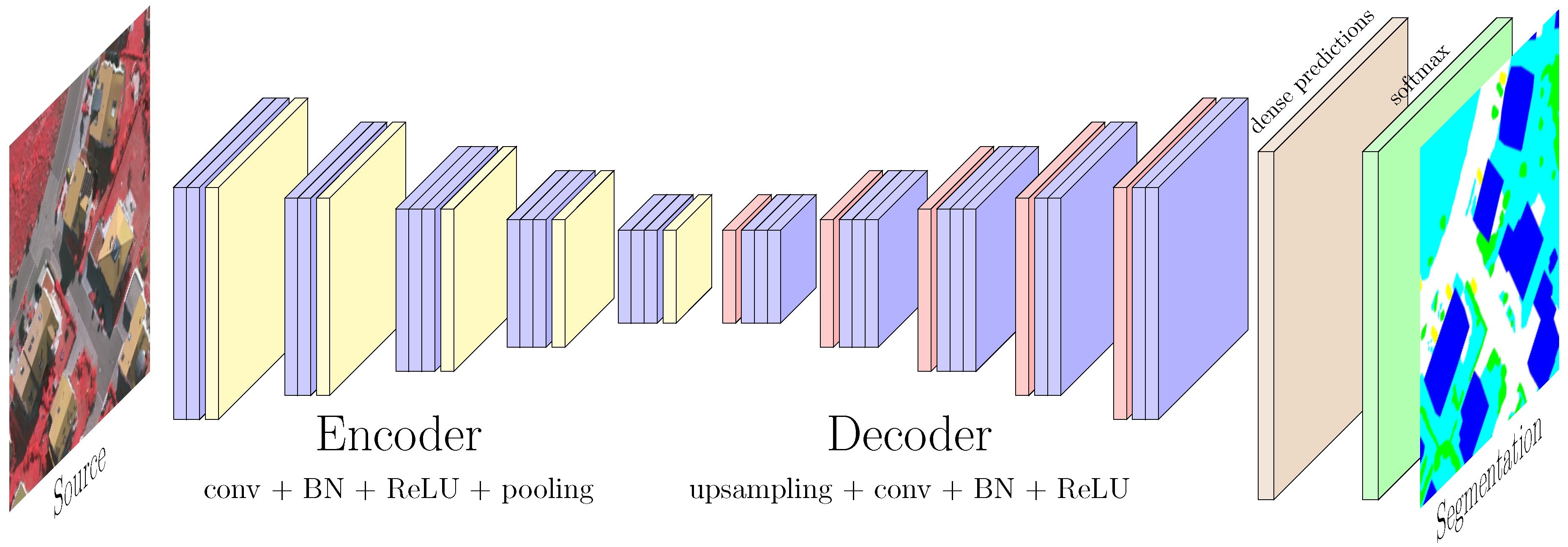
Figure 3.
Data augmentation on a vehicle from the VEDAI dataset. (a) original; (b) 90° rotation; (c) 180° rotation; (d) up/down flip; (e) left/right flip; (f) zoom; (g) translation.
Figure 3.
Data augmentation on a vehicle from the VEDAI dataset. (a) original; (b) 90° rotation; (c) 180° rotation; (d) up/down flip; (e) left/right flip; (f) zoom; (g) translation.

Figure 4.
Excerpts from the datasets used for vehicle analysis. (a) ISPRS Potsdam dataset (RGB); (b) NZAM/ONERA Christchurch dataset (RGB).
Figure 4.
Excerpts from the datasets used for vehicle analysis. (a) ISPRS Potsdam dataset (RGB); (b) NZAM/ONERA Christchurch dataset (RGB).

Figure 5.
Segmentation results (top row: NZAM/ONERA Christchurch, bottom row: ISPRS Potsdam). (a) RGB image, (b) Ground truth, (c) SegNet prediction. Legend: white: impervious surfaces; blue: buildings; cyan: low vegetation; green: trees; yellow: vehicles; red: clutter; black: undefined.
Figure 5.
Segmentation results (top row: NZAM/ONERA Christchurch, bottom row: ISPRS Potsdam). (a) RGB image, (b) Ground truth, (c) SegNet prediction. Legend: white: impervious surfaces; blue: buildings; cyan: low vegetation; green: trees; yellow: vehicles; red: clutter; black: undefined.
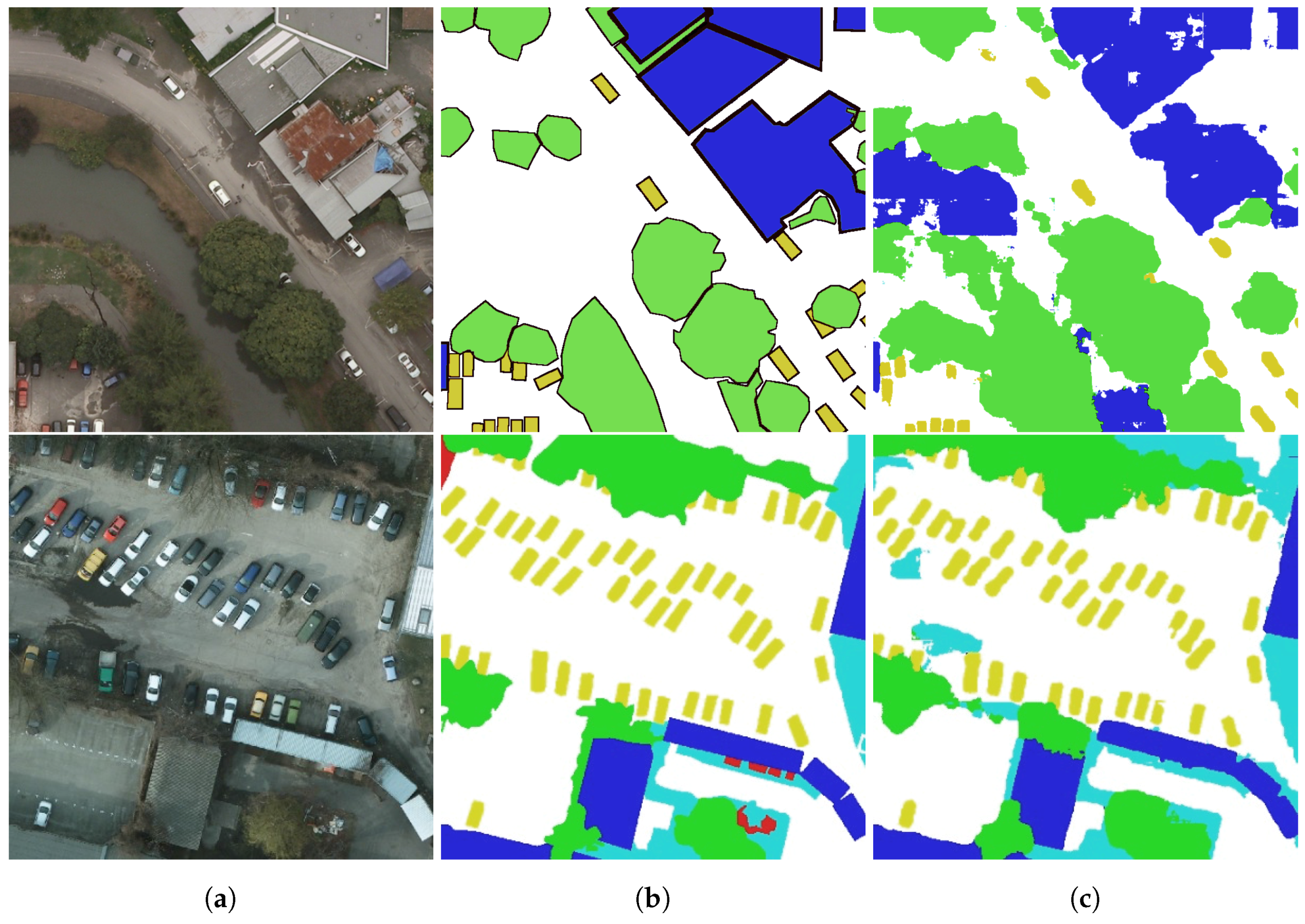
Figure 6.
Detection samples on ISPRS Potsdam and NZAM/ONERA Christchurch (true positives are in green, false positives in red and real bounding boxes in blue). (a) vehicle detection on Christchurch; (b) vehicle detection on Christchurch; (c) vehicle detection on Potsdam.
Figure 6.
Detection samples on ISPRS Potsdam and NZAM/ONERA Christchurch (true positives are in green, false positives in red and real bounding boxes in blue). (a) vehicle detection on Christchurch; (b) vehicle detection on Christchurch; (c) vehicle detection on Potsdam.
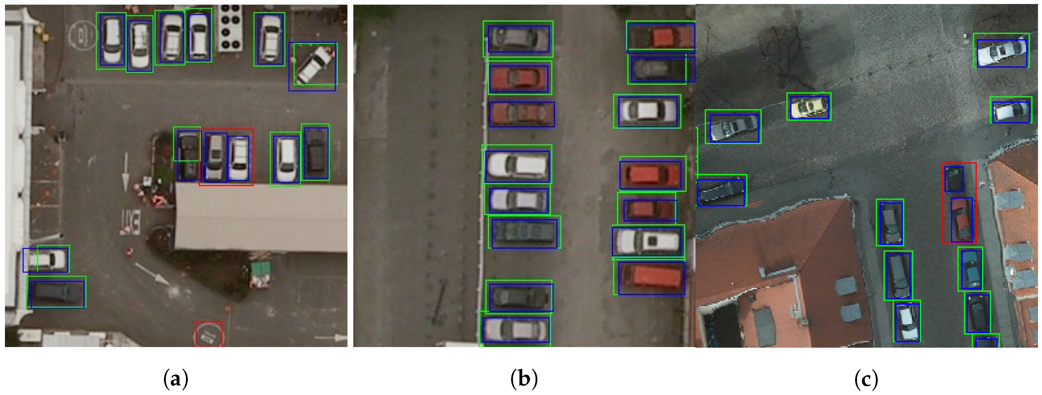
Figure 7.
Successful segmentation but misclassified vehicles in the Potsdam dataset. (a) van predicted as truck; (b) van predicted as truck; (c) car (SUV) predicted as van; (d) pick up predicted as van.
Figure 7.
Successful segmentation but misclassified vehicles in the Potsdam dataset. (a) van predicted as truck; (b) van predicted as truck; (c) car (SUV) predicted as van; (d) pick up predicted as van.

Figure 8.
Successful segmentation and classification of vehicles in the Potsdam dataset. (a) pick up; (b) van; (c) truck; (d) car.
Figure 8.
Successful segmentation and classification of vehicles in the Potsdam dataset. (a) pick up; (b) van; (c) truck; (d) car.
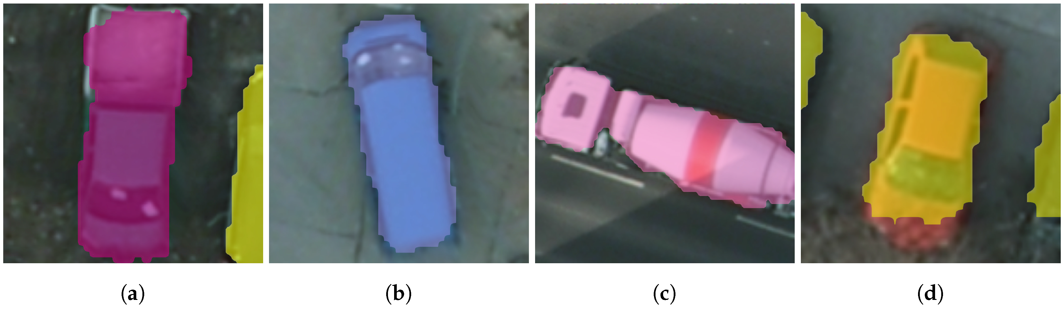
Figure 9.
Visualizing vehicles in the ISPRS Potsdam dataset (best viewed in color). (a) RGB data (Potsdam); (b) vehicle density map (Potsdam); (c) vehicle ground truth (Potsdam); (d) predicted vehicles (Potsdam).
Figure 9.
Visualizing vehicles in the ISPRS Potsdam dataset (best viewed in color). (a) RGB data (Potsdam); (b) vehicle density map (Potsdam); (c) vehicle ground truth (Potsdam); (d) predicted vehicles (Potsdam).

Figure 10.
Visualizing vehicles in the NZAM/ONERA Christchurch dataset (best viewed in color). (a) RGB data (Christchurch); (b) vehicle density map (Christchurch); (c) vehicle ground truth (Christchurch); (d) predicted vehicles (Christchurch).
Figure 10.
Visualizing vehicles in the NZAM/ONERA Christchurch dataset (best viewed in color). (a) RGB data (Christchurch); (b) vehicle density map (Christchurch); (c) vehicle ground truth (Christchurch); (d) predicted vehicles (Christchurch).


Table 1.
Vehicle counts by class in the presented datasets.
| Dataset/Class | Car | Truck | Van | Pickup | Boat | Camping Car | Other | Plane | Tractor |
|---|---|---|---|---|---|---|---|---|---|
| VEDAI | 1340 | 300 | 100 | 950 | 170 | 390 | 200 | 47 | 190 |
| NZAM/ONERA Christchurch | 2267 | 73 | 120 | 90 | - | - | - | - | - |
| ISPRS Potsdam | 1990 | 33 | 181 | 40 | - | - | - | - | - |
Table 2.
Semantic segmentation results on the Potsdam dataset (F1 scores and overall accuracy (OA)).
Table 2.
Semantic segmentation results on the Potsdam dataset (F1 scores and overall accuracy (OA)).
| Dataset | Method | Imp. Surfaces | Building | Low veg. | Tree | Cars | OA |
|---|---|---|---|---|---|---|---|
| Validation 12.5cm/px | SegNet RGB | 92.4% ± 0.6 | 95.8% ± 1.9 | 85.8% ± 1.3 | 83.0% ± 2.1 | 95.7% ± 0.3 | 90.6% ± 0.6 |
| Test 5cm/px | SegNet IRRG | 92.4% | 95.8% | 86.7% | 87.4% | 95.1% | 90.0% |
| FCN + CRF [17] | 91.8% | 95.9% | 86.3% | 87.7% | 89.2% | 89.7% | |
| ResNet-101 [CASIA] | 92.8% | 96.9% | 86.0% | 88.2% | 94.2% | 89.6% |
Table 3.
Semantic segmentation results on the Christchurch dataset (pixel-wise accuracies).
| Source | Background | Building | Vegetation | Vehicle | OA |
|---|---|---|---|---|---|
| RGB | 75.6% ± 8.9 | 91.7% ± 1.3 | 55.2% ± 11.6 | 61.9% ± 2.4 | 84.4% ± 2.6 |
Table 4.
Instance segmentation and vehicle detection results for different morphological preprocessing (mean intersection over union (mIoU), precision and recall).
Table 4.
Instance segmentation and vehicle detection results for different morphological preprocessing (mean intersection over union (mIoU), precision and recall).
| Dataset | Preprocessing | mIoU | Precision | Recall |
|---|---|---|---|---|
| NZAM/ONERA Christchurch | ∅ | 60.0% | 0.597 | 0.797 |
| Opening | 69.8% | 0.817 | 0.791 | |
| Opening + remove small objects | 70.7% | 0.833 | 0.791 | |
| ISPRS Potsdam | ∅ | 70.1% | 0.748 | 0.842 |
| Opening | 73.3% | 0.866 | 0.842 | |
| Opening + remove small objects | 74.2% | 0.907 | 0.841 |
Table 5.
Vehicle detection results on the ISPRS Potsdam and NZAM/ONERA datasets.
| Dataset | Method | Precision | Recall |
|---|---|---|---|
| NZAM/ONERA Christchurch | HOG + SVM [20] | 0.402 | 0.398 |
| DtMM (5 models) [24] | 0.743 | 0.737 | |
| Ours | 0.833 | 0.791 | |
| ISPRS Potsdam | Ours | 0.907 | 0.841 |
Table 6.
Classification results of various CNN on VEDAI (in %).
| Model | Car | Truck | Ship | Tractor | Camping Car | Van | Pickup | Plane | Vehicle | OA | Time (ms) |
|---|---|---|---|---|---|---|---|---|---|---|---|
| LeNet | 74.3 | 54.4 | 31.0 | 61.1 | 85.9 | 38.3 | 67.7 | 13.0 | 47.5 | 66.3 ± 1.7 | 2.1 |
| AlexNet | 91.0 | 84.8 | 81.4 | 83.3 | 98.0 | 71.1 | 85.2 | 91.4 | 77.8 | 87.5 ± 1.5 | 5.7 |
| VGG-16 | 90.2 | 86.9 | 86.9 | 86.5 | 99.6 | 71.1 | 91.4 | 100.0 | 77.2 | 89.7 ± 1.5 | 31.7 |
Table 7.
Classification results on VEDAI using AlexNet with several preprocessing (in %).
| Model | Car | Truck | Ship | Tractor | Camping Car | Van | Pickup | Plane | Vehicle | OA | AA |
|---|---|---|---|---|---|---|---|---|---|---|---|
| Baseline | 90.4 | 66.7 | 80.4 | 89.5 | 96.6 | 63.3 | 78.7 | 92.6 | 75.0 | 83.9 ± 2.7 | 81.5 ± 1.9 |
| DA | 88.2 | 82.2 | 78.4 | 82.5 | 97.4 | 63.3 | 85.1 | 66.7 | 73.3 | 85.6 ± 1.4 | 77.3 ± 8.7 |
| R | 87.9 | 71.1 | 86.3 | 84.2 | 97.4 | 73.3 | 87.2 | 100.0 | 75.0 | 86.1 ± 0.9 | 84.7 ± 1.7 |
| DA + R | 91.4 | 85.6 | 88.2 | 87.6 | 97.4 | 70.0 | 87.2 | 100.0 | 81.7 | 89.0 ± 0.5 | 87.7 ± 1.5 |
DA = data augmentation, R = renormalization.
Table 8.
Classification results on the enhanced vehicle ground truths.
| Dataset | Classifier | Car | Van | Truck | Pick up | OA | AA |
|---|---|---|---|---|---|---|---|
| Potsdam | Cars only | 100% | 0% | 0% | 0% | 94% | 25% |
| AlexNet | 98% | 66% | 67% | 0% | 95% | 58% | |
| VGG-16 | 92% | 66% | 75% | 33% | 89% | 67% | |
| Christchurch | Cars only | 100% | 0% | 0% | 0% | 94% | 25% |
| AlexNet | 94% | 40% | 67% | 89% | 93% | 73% | |
| VGG-16 | 97% | 80% | 67% | 78% | 96% | 80% |
Table 9.
Average error when estimating the number of vehicles in 125×125 m2 area.
| Dataset | ISPRS Potsdam | NZAM/ONERA Christchurch |
|---|---|---|
| Absolute error (average error/ground truth total) | 3/52 | 6/66 |
| Relative error | 7.9% | 9.1% |
© 2017 by the authors. Licensee MDPI, Basel, Switzerland. This article is an open access article distributed under the terms and conditions of the Creative Commons Attribution (CC BY) license (http://creativecommons.org/licenses/by/4.0/).
Share and Cite
MDPI and ACS Style
Audebert, N.; Le Saux, B.; Lefèvre, S. Segment-before-Detect: Vehicle Detection and Classification through Semantic Segmentation of Aerial Images. Remote Sens. 2017, 9, 368. https://doi.org/10.3390/rs9040368
AMA Style
Audebert N, Le Saux B, Lefèvre S. Segment-before-Detect: Vehicle Detection and Classification through Semantic Segmentation of Aerial Images. Remote Sensing. 2017; 9(4):368. https://doi.org/10.3390/rs9040368
Chicago/Turabian StyleAudebert, Nicolas, Bertrand Le Saux, and Sébastien Lefèvre. 2017. "Segment-before-Detect: Vehicle Detection and Classification through Semantic Segmentation of Aerial Images" Remote Sensing 9, no. 4: 368. https://doi.org/10.3390/rs9040368
Note that from the first issue of 2016, this journal uses article numbers instead of page numbers. See further details here.