
An ML-Based Radial Velocity Estimation Algorithm for Moving Targets in Spaceborne High-Resolution and Wide-Swath SAR Systems


1
Key Laboratory of Technology in Geo-Spatial Information Processing and Application System, Institute of Electronics, Chinese Academy of Sciences, Beijing 100190 China
2
University of the Chinese Academy of Sciences, Beijing 100049, China
*
Author to whom correspondence should be addressed.
Remote Sens. 2017, 9(5), 404; https://doi.org/10.3390/rs9050404
Submission received: 28 February 2017
/
Revised: 20 April 2017
/
Accepted: 21 April 2017
/
Published: 26 April 2017
(This article belongs to the Special Issue Ocean Remote Sensing with Synthetic Aperture Radar)
Abstract
:Multichannel synthetic aperture radar (SAR) is a significant breakthrough to the inherent limitation between high-resolution and wide-swath (HRWS) compared with conventional SAR. Moving target indication (MTI) is an important application of spaceborne HRWS SAR systems. In contrast to previous studies of SAR MTI, the HRWS SAR mainly faces the problem of under-sampled data of each channel, causing single-channel imaging and processing to be infeasible. In this study, the estimation of velocity is equivalent to the estimation of the cone angle according to their relationship. The maximum likelihood (ML) based algorithm is proposed to estimate the radial velocity in the existence of Doppler ambiguities. After that, the signal reconstruction and compensation for the phase offset caused by radial velocity are processed for a moving target. Finally, the traditional imaging algorithm is applied to obtain a focused moving target image. Experiments are conducted to evaluate the accuracy and effectiveness of the estimator under different signal-to-noise ratios (SNR). Furthermore, the performance is analyzed with respect to the motion ship that experiences interference due to different distributions of sea clutter. The results verify that the proposed algorithm is accurate and efficient with low computational complexity. This paper aims at providing a solution to the velocity estimation problem in the future HRWS SAR systems with multiple receive channels.
1. Introduction
Remote sensing for civilian and military applications sets a high requirement on both the spatial resolution and swath coverage for synthetic aperture radar (SAR). However, conventional SAR systems can barely achieve high-resolution and wide-swath (HRWS) images simultaneously [1]. Higher pulse repetition frequency (PRF) is needed to obtain higher azimuth resolution, while lower PRF is required to acquire a wider range swath. Multichannel SAR in the azimuth, which can overcome this inherent limitation, has attracted much attention in recent years [2]. The launch of the TerraSAR-X satellite in 2007 [3], the ALOS-2 satellite in 2014 [4], and the Chinese Gaofen-3 satellite in 2016, which all contain a dual-receive channel mode, demonstrated the feasibility of this technique. Spaceborne HRWS SAR with more receive channels is one of the prospects of SAR systems. Moving target indication and imaging is one of the primary applications of spaceborne HRWS SAR systems, especially for ocean remote sensing [2,3]. Estimation of the target’s velocity is crucial for target relocation, focused imaging and false target suppression [5,6,7,8,9,10,11,12,13,14,15].
The moving target’s velocity can be divided into the radial velocity and the azimuth velocity, which stands for the cross-track and along-track velocities of the moving target, respectively. For a spaceborne HRWS SAR system, the azimuth velocity of a motion target is far smaller than that of the satellite, and thus can be ignored. The effects of the radial velocity are predominant [11], and are listed as follows:
- (1)
- The linear Range Cell Migration (RCM) is caused by the radial velocity after range compression of the moving target;
- (2)
- The azimuth offset of a moving target’s location is proportional to its radial velocity; and
- (3)
- The reconstructed echo of a moving target will introduce a frequency-dependent phase mismatch, leading to false targets along the azimuth after imaging.
Thus, estimating the radial velocity is a key procedure to relocation and precise imaging of a moving target.
For a spaceborne multichannel SAR, the low PRF is transmitted to achieve wide swath images with low range ambiguity levels, at the cost of under-sampled data in the azimuth and Doppler spectrum ambiguity for a single channel. Unambiguous imaging of a single channel echo is not feasible. Therefore, a reconstruction algorithm is introduced [1] to suppress the Doppler spectrum ambiguity before obtaining a HRWS image. Most of the previous studies place an emphasis on moving target indication (MTI) with the assumption that there is no Doppler ambiguity for each channel. For example, in the along-track interferometry (ATI) method [6], the Eigen-decomposition method of the covariance matrix [7] processes in the image domain of each channel. However, the main problem of a HRWS SAR MTI system is under-sampled data in the azimuth for signal-channel echo.
In recent years, several methods have been proposed that are focused on moving target indication for HRWS SAR systems, which aim at estimating velocity before imaging. In [8], estimating the radial velocity is transformed to the direction-of-arrival (DOA) estimation of the echoes. By constructing the spatial spectrum of the moving target, the radial velocity can be estimated by maximizing the spectrum. However, without analyzing the efficiency or considering the sea clutter, the analysis is not comprehensive. In [9,10,11], the imagery quality of the moving target is weighed by some criterion, and the radial velocity is estimated by searching for the value which optimizes the imagery quality. These approaches need iteration, thus guaranteeing the accuracy with the sacrifice of efficiency.
In [12], the Radon transform is applied to estimate the slope of the Doppler spectrum of the single-channel echo, and the radial velocity is proportional to the slope. The computational load is large for the implementation of Radon transform with each searched velocity. Additionally, the redundant information of the multi-channel signal is not taken full advantage of. Yang et al. and Wang et al. [13,14] transform the velocity estimation problem to measuring the azimuth offset, which is proportional to its radial velocity mentioned above. However, these methods need additional processing of the image and determination between false targets and the real one. Furthermore, these methods lack detailed analysis of performance under sea clutter distributions.
In this paper, we propose a novel algorithm for velocity estimation and unambiguous imaging of the moving target in a spaceborne HRWS SAR system. In addition, the estimation accuracy under different sea clutter distributions are discussed. Firstly, we deduce the echo of a moving target for multichannel SAR systems, and obtain the relationship of the radial velocity and the cone angle. Considering that the cone angles are sparse in space for a certain Doppler frequency [16], we apply the maximum likelihood (ML) method to estimate the cone angle as well as the radial velocity. Then the signal reconstruction and compensation of the phase mismatch caused by target motion are processed, followed by focused imaging to suppress false targets. Finally, we discuss the estimation of a moving ship interfered with different sea clutter distributions. The merit of this algorithm is that it does not need iteration or Eigen-decomposition, thus the computational complexity is not large. More importantly, this algorithm can estimate velocities of multiple moving targets as it does not need too many samples of Doppler bins, making estimating of adjacent targets possible.
This paper begins with signal model of the moving target for a HRWS SAR system in Section 2. In Section 3, detailed descriptions of the proposed velocity estimation algorithm and the imaging process of multichannel moving target echoes are given, and the Cramér-Rao lower bound of velocity estimation is deduced. Section 4 presents the experimental results of estimation accuracy under different conditions, followed by the performance analysis in Section 5. Section 6 draws conclusions and discusses future perspectives.
2. Echo Model of the Moving Target
2.1. Ideal Echo Model
For spaceborne multichannel SAR systems, the echo of the moving target has the following characteristics:
- The velocity of the moving target is treated as constant during the antenna beam scanning as the satellite is moving fast.
- The azimuth velocity of the moving target is negligible as it is much smaller than the satellite velocity.
- The radial velocity can be treated as the same for each receive channel as the radar beam is very narrow.
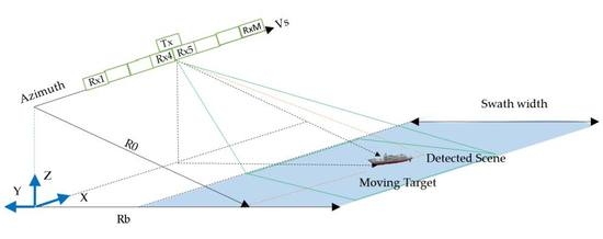
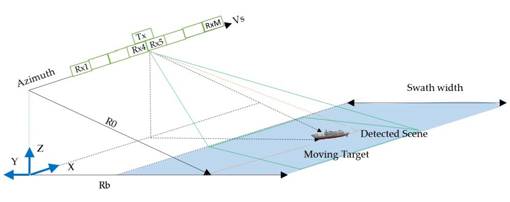
The geometry of the HRWS SAR system is depicted in Figure 1. The x-axis points to the direction of the platform velocity of the satellite, the z-axis points away from the Earth’s center, and the three axes satisfy the orthogonal right-hand rule. The velocity of the platform is , is the shortest slant distance of the target, and is the corresponding ground range. The full area of the antenna is used as the transmitter, and is split into M channels in the azimuth as receivers. The antenna transmits chirp signals at the center (Tx), and Rx1-RxM receive echoes simultaneously. The azimuth resolution of the multichannel SAR system depends on the aperture size of a single receive channel. The distance between two receive channels is d, the radial velocity and the azimuth velocity of the moving target are and , respectively.
The distance between the transmit center and the moving target is donated as , and the distance between the m-th receiver and the moving target is , expressed as:
where denote the range time and azimuth time, respectively, and:
For the sake of convenient expression, the moving target is modeled as an ideal point target with constant radar cross section (RCS). Then the received signal of the m-th channel can be expressed as:
where c is the speed of light, is the synthetic aperture time, and and are the pulse width and chirp rate, respectively. stands for the overall amplitude weighting of the target, containing the target backscatter coefficient, the weighted coefficient of the antenna pattern, and weighting factors of electromagnetic wave propagation in space. Substituting Equations (1) and (2) into Equation (4), the Doppler centroid and the Doppler rate can be written as:
While for a static target or clutter, , the Doppler centroid and the Doppler rate are
Define and as the cone angles of the clutter and the moving target, respectively. From Equations (5) and (6), the existence of the target motion result in a certain offset of the Doppler frequency. For a side-looking SAR system, the relationship of the Doppler frequency and the cone angle can be expressed as [8]:
Figure 2a shows the linear relationship between and , where the dotted line indicates the clutter, and the solid line the ground moving target. For a HRWS SAR system, a low PRF is adopted to eliminate the range ambiguities and enlarge the coverage, at the cost of the Doppler ambiguity. Then the relationship between and is shown as Figure 2b in practical applications, where the Doppler spectrum of the clutter and the moving target are both folded. The corresponding moving target signal of the m-th channel in the Doppler domain is expressed as:
where is echo of the m-th channel in the range-Doppler domain, is the PRF, and the number of the main Doppler spectrum ambiguity is N, N = 2L + 1.
2.2. Echo Model with Clutter and Noise
In reality, the SAR echoes of the moving target are interfered by clutter and noise; the clutter is the background of the detected scene, and the noise comes from the receive chain of each channel. Thus the model of the clutter depends on the detected scene, and the model of the noise is normally white Gaussian noise. Considering the clutter and the noise, the echo in the range-Doppler domain of the m-th channel can be expressed as:
where is the clutter signal of the first channel in the range-Doppler domain, is the white Gaussian noise.
For simplification, the echoes of M channels in the vector form can be written as [17]
where bold lowercase letters are used for vectors, denotes the echo vector in the range-Doppler domain of M channels, and is the echo of the i-th channel combined with clutter and noise. denotes the echo vector of moving target, denotes the echo vector of clutter, and n denotes the echo vector of thermal noise. and are the complex scattering coefficients of the moving target and the clutter unit, respectively.
3. The Proposed Velocity Estimation Algorithm
According to Equation (8), the existence of causes a certain offset of the Doppler frequency; thus, the cone angle of the moving target for a certain Doppler bin is related to . In other words, the problem of radial velocity estimation is equivalent to the problem of cone angle estimation. Different from traditional direction of arrival (DOA) estimation, there exists a Doppler ambiguity in the echo for the HRWS SAR system. Fortunately, the steering vector matrix can be constructed considering the Doppler ambiguity for the sparse signal representation.
In this section, we firstly describe the proposed ML-based algorithm. Then the Cramér-Rao lower bound of velocity estimation is deduced. Finally, the HRWS SAR moving target imaging procedure is presented.
3.1. Algorithm Discription
To transform the velocity estimation problem to the cone angle estimation, or the steering vector estimation, the echo expressed in Equation (9) can be rewritten in the vector form as the product of the echo of first channel and the steering vector matrix, i.e.,
where,
is the l-th ambiguous component of the first channel signal, and denotes the l-th ambiguous steering vector, i.e.,
where
From Equation (17), there is a one-to-one correspondence between radial velocity and the cone angle for a moving target.
Then the maximum likelihood (ML) algorithm is applied to estimate or . The requirements of the ML algorithm are as follows [18]:
- The signal covariance matrix is positive definite;
- The number of sampling points is larger than the number of receive channels; and
- The noises sampled at different Doppler frequencies are uncorrelated, and obey a white Gaussian distribution.
The joint conditional probability density function of the sampled signals from K Doppler frequencies is:
where is the average power of , is the sampled value of Equation (11), and is the sampled value of moving target signals in range-Doppler domain, i.e., .
The criterion of the ML estimator is maximizing the following cost function
where represents the trace of a matrix, is the steering vector matrix in Equation (15), and is the signal covariance matrix of . By searching for in a certain space and computing the steering vector matrix , the maximum likelihood spectrum can be calculated. The maximum value of the spectrum corresponds to the ML estimation of .
The process of the estimator is as follows:
- (1)
- Conduct range compression of the echo of each channel, Equation (4) turns intowhere is the bandwidth of the chirp signal. As the sinc function varies little around the maximum value, the sinc function of Equation (20) for each channel is approximately equal.
- (2)
- Conduct the azimuth Fourier transform, then extract the trajectory of the moving target in the range-Doppler domain. Sample the extracted signal at K Doppler bins to constitute vector , i.e.,whereThe signal covariance matrix is acquired by .
- (3)
- For each searched , compute the steering vector matrix . Find the ML estimation of by substituting and into Equation (19). Finally, average the estimated values from K Doppler bins to improve the robustness.
The common point of the proposed algorithm and the Capon spectrum [7] and MUSIC algorithms [8] is that, they all search for the best radial velocity according to some principle by constructing the sampled signal covariance matrix. The difference is the criterion they are based on. The proposed ML-based algorithm has lower complexity than the iterative approaches in [9,10,11], which need imaging for each possible velocity during the iteration. Moreover, this algorithm can estimate velocities of multiple moving targets as it does not need a large number of Doppler bins, as long as the number is larger than that of the receive channels.
3.2. The Cramér-Rao Lower Bound of Velocity Estimation
The Cramér–Rao lower bound (CRLB) is an important evaluation indicator for the effectiveness of parameter estimation. There inevitably exist errors in the ML estimation of . The root mean squired error (RMSE) of estimation is compared with the CRLB, and the estimator is viewed as an effective estimate if the RMSE infinitely approaches CRLB with the increase of the signal-to-noise ratio (SNR).
A classical tool for deriving the CRLB is the Fisher information matrix (FIM), and the CRLB is obtained by computing the inverse of the FIM [19]. The FIM is obtained from the second-order derivative of the likelihood function, which is the logarithm of the joint conditional probability density function in Equation (18).
where is the vector constituted by the sampled signals.
From Equation (18), the likelihood function is:
It has been proven in [20] that the CRLB of the ML estimation of the cone angle is expressed as
where:
In Equation (26), is the derivative of the steering vector to the cone angle, i.e.,
Finally, the CRLB of estimation is obtained from the relationship of and in Equation (17), i.e.,
3.3. Processing Flow
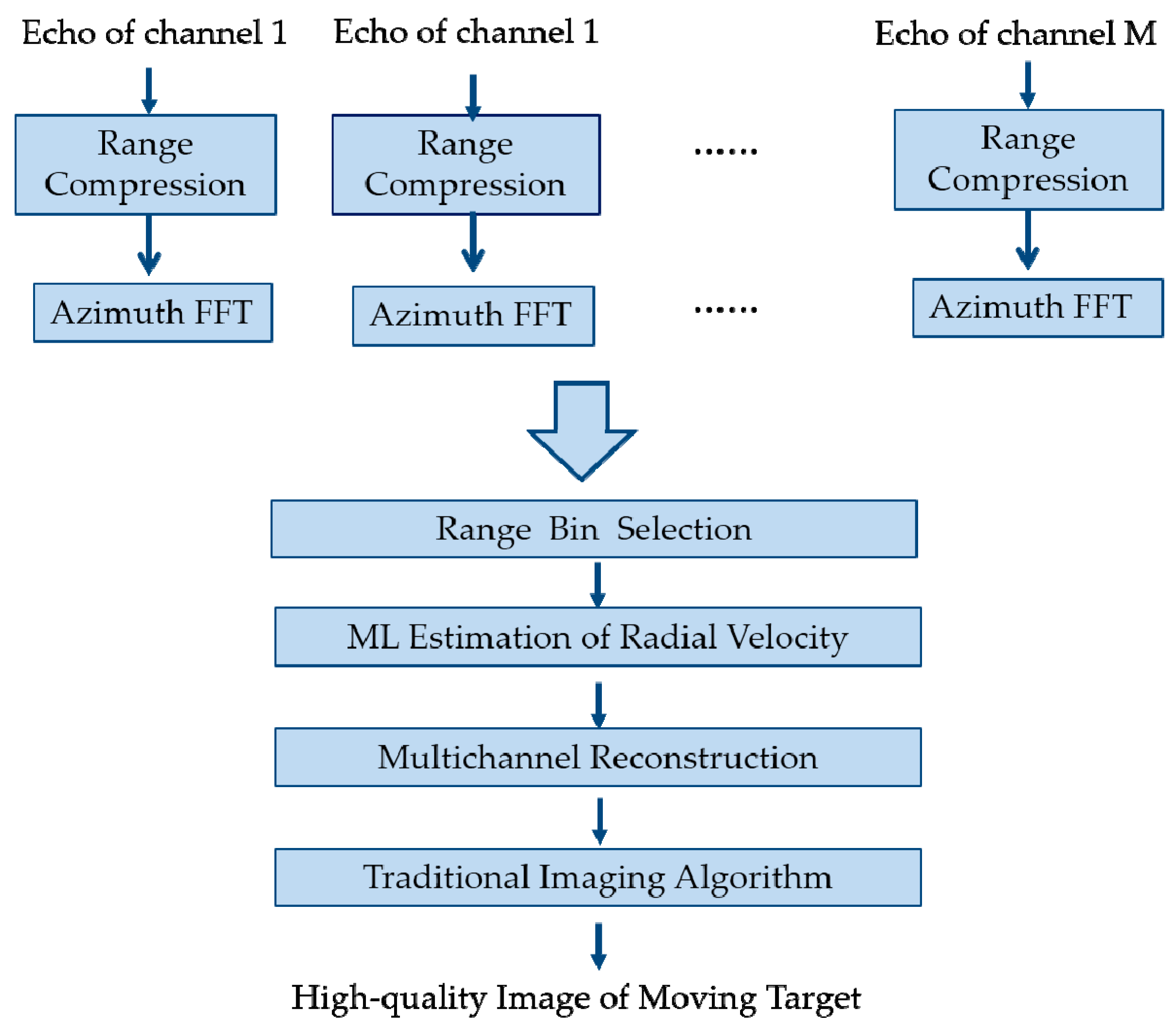
In Section 3.1, the proposed ML-based algorithm is described to estimate the radial velocity. Then the phase errors caused by the moving target of the M channels are compensated before imaging to suppress the false targets. The total processing flow of the moving target’s echoes of the multichannel SAR system is illustrated in Figure 3. Detailed descriptions are as follows:
- Range Compression: Conduct range compression with the echo of each channel.
- Azimuth Fourier Transform: Perform the Fourier transform in the azimuth to obtain
- Range Bin Selection: Choose the range bins that contain echoes of the moving target. Normally, the range bin of the peak value and its adjacent range bins are selected.
- ML Estimation of Radial Velocity: The ML method discussed in Section 3.1 is applied to estimate the radial velocity of the moving target.
- Multichannel Reconstruction: Reconstruct echoes of M channels and compensate for the phase offsets introduced by target motion.
- Traditional Imaging Algorithm: After reconstruction, the echoes of M channels are combined to equivalent single-channel signal without Doppler ambiguities. The traditional chirp scaling (CS) algorithm can be applied to obtain a focused image of the moving target with suppression of the false targets.
4. Experimental Results
In this section, experiments are conducted to evaluate the performance of the proposed ML-based radial velocity estimator. In Section 4.1, we demonstrate the accuracy and the effectiveness of the algorithm, the accuracy is evaluated by the estimation error, and the effectiveness is evaluated by the proximity of the RMSE to the CRLB. After radial velocity estimation, phase offsets among channels caused by target motion are compensated before imaging. The imaging results before and after compensation are compared in Section 4.2. Finally, the estimation accuracy under different distributions of sea clutter is discussed in Section 4.3.
The echo model of the moving target for the HRWS SAR system is shown is Figure 1. Figure 4 shows a diagram of the transmitting and receiving centers. The parameters of the simulated spaceborne multichannel SAR system are listed in Table 1. The number of the Doppler ambiguity N equals 5 according to the parameters.
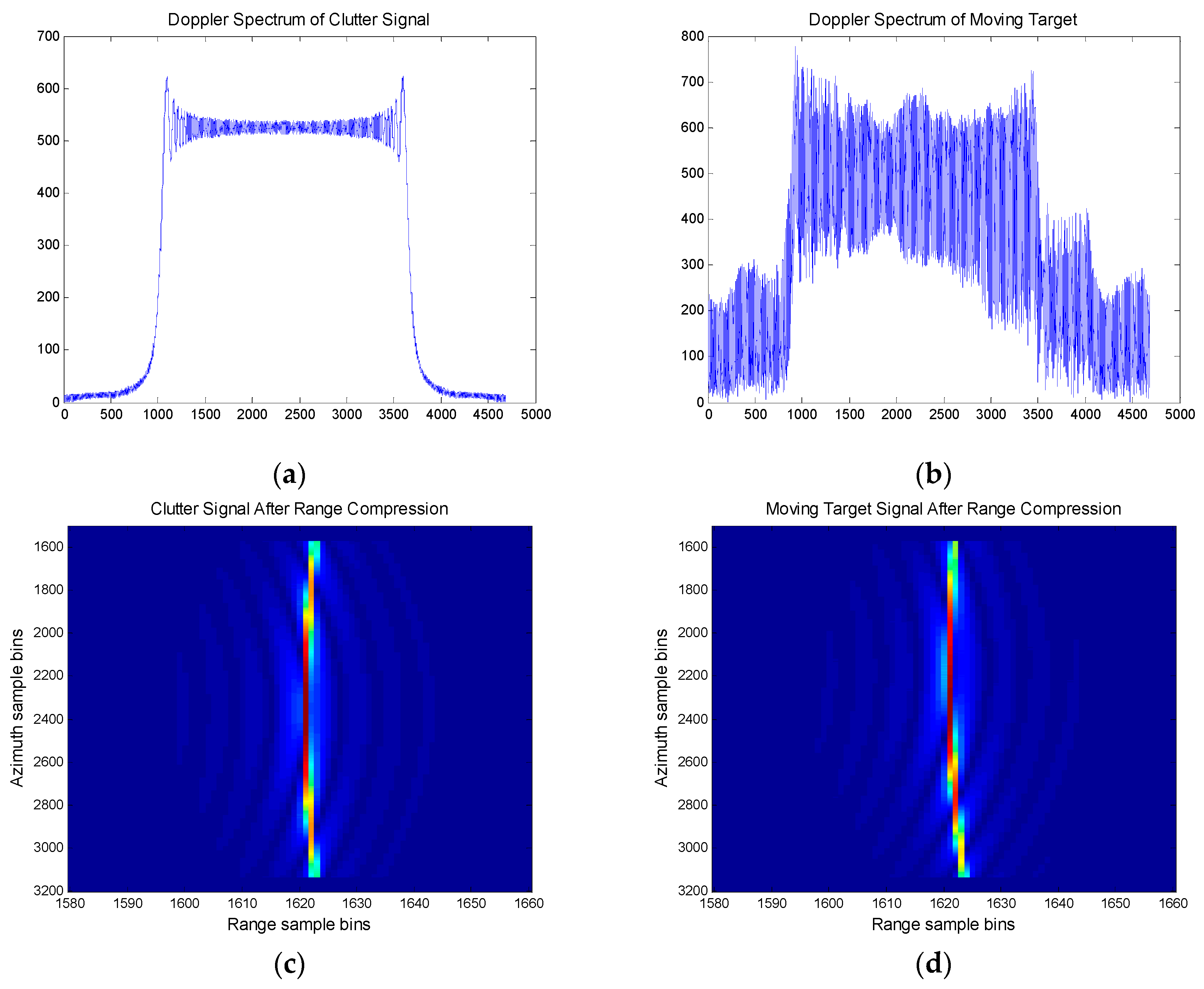
Figure 5 shows the comparison of simulated clutter signal and the moving target whose radial velocity is 10 m/s. Figure 5a is the Doppler spectrum of the clutter signal of reconstructed echoes, compared to that of the moving target signal in Figure 5b, where the spectral errors are evident from the frequency-dependent phase mismatch caused by radial velocity. Figure 5c,d compare the trajectory of the clutter signal and the moving target after range compression. We can see an additional linear Range Cell Migration (RCM) after range compression of the moving target. In the following, the trajectory of the moving target is extracted to estimate the radial velocity.
4.1. Performance of Radial Velocity Estimaion
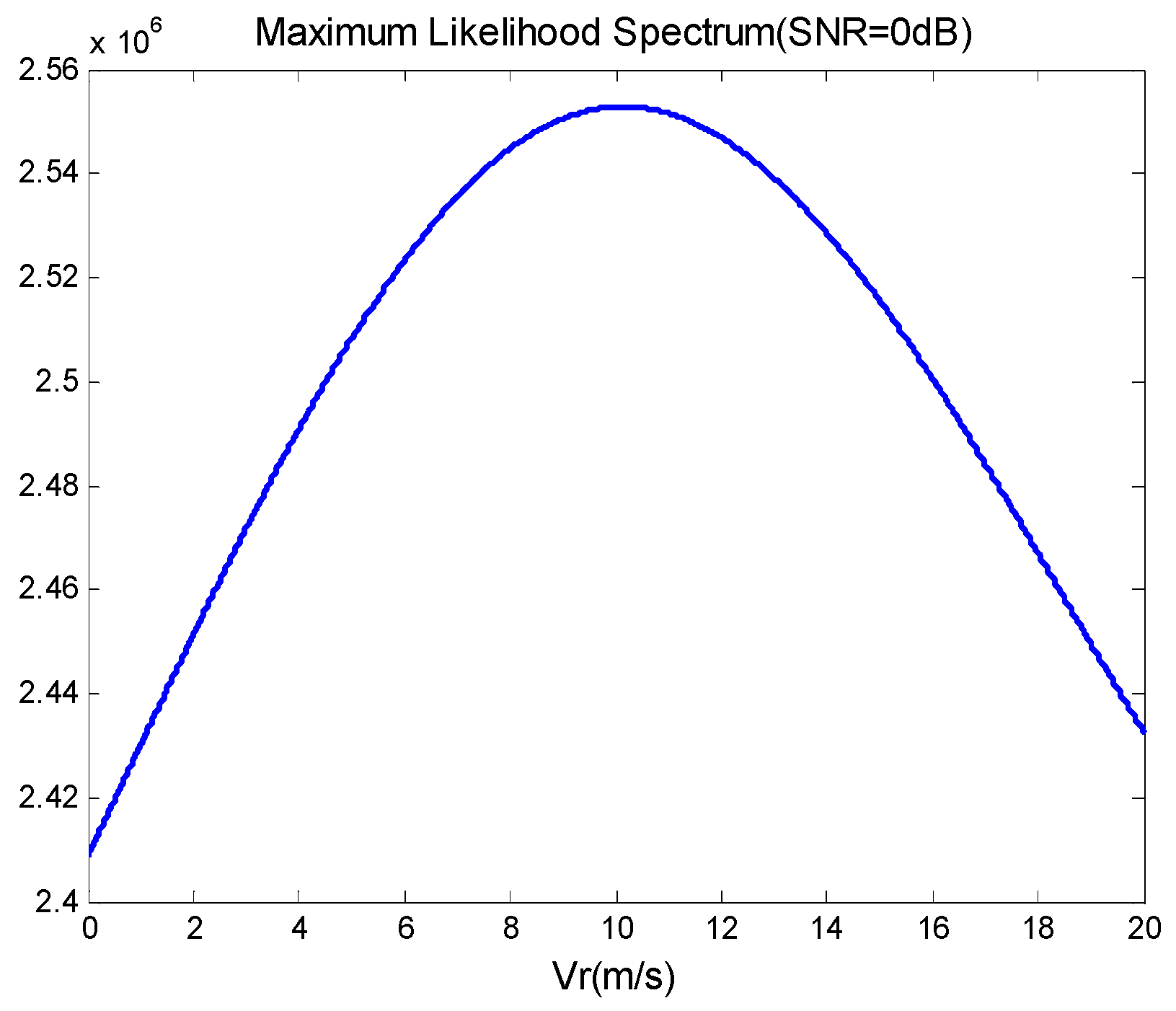
In order to verify the performance of the proposed ML-based algorithm, an experiment is conducted to evaluate the estimation accuracy and efficiency under different signal-to-noise ratios (SNR). In the simulation, the radial velocity of the moving target is 10 m/s, and the SNR varies from −5 dB to 20 dB. The searching step is 0.01 m/s and the searching range is 0–20 m/s. The clutter scenario is temporarily not considered in the subsection. In the experiment, the range bin of the peak value from the trajectory of the moving target and its adjacent 10 range bins are selected, and we average the estimated values from 60 Doppler bins to improve the robustness. The estimated radial velocities, the estimation errors and relative errors under different SNRs are listed in Table 2. The maximum likelihood spectrum of radial velocity with the SNR = 0 dB is illustrated in Figure 6.
In the following, the efficiency of the estimator is evaluated by the proximity of RMSE to the CRLB. RMSE is expressed as
where I is the number of Monte Carlo experiments. In the comparison, we take the square root of the CRLB in Equation (28). As the computational load is high, 100 Monte Carlo experiments are conducted in the simulation. The RMSE is compared with the CRLB under different SNRs in Figure 7.
From the results in Table 2, the ML-based algorithm can estimate the radial velocity under very strong noise conditions. As a general rule, the SNR is larger than 0 dB, the estimation error is smaller than 0.22 m/s, with the relative error smaller than 2.2%. From the comparison of the RMSE and the CRLB in Figure 7, the RMSE infinitely approaches the CRLB with the increase of the SNR. Thus, the proposed ML-based radial velocity estimator is proven to be effective.
4.2. Imaging Results Before and after Estimation and Compensation
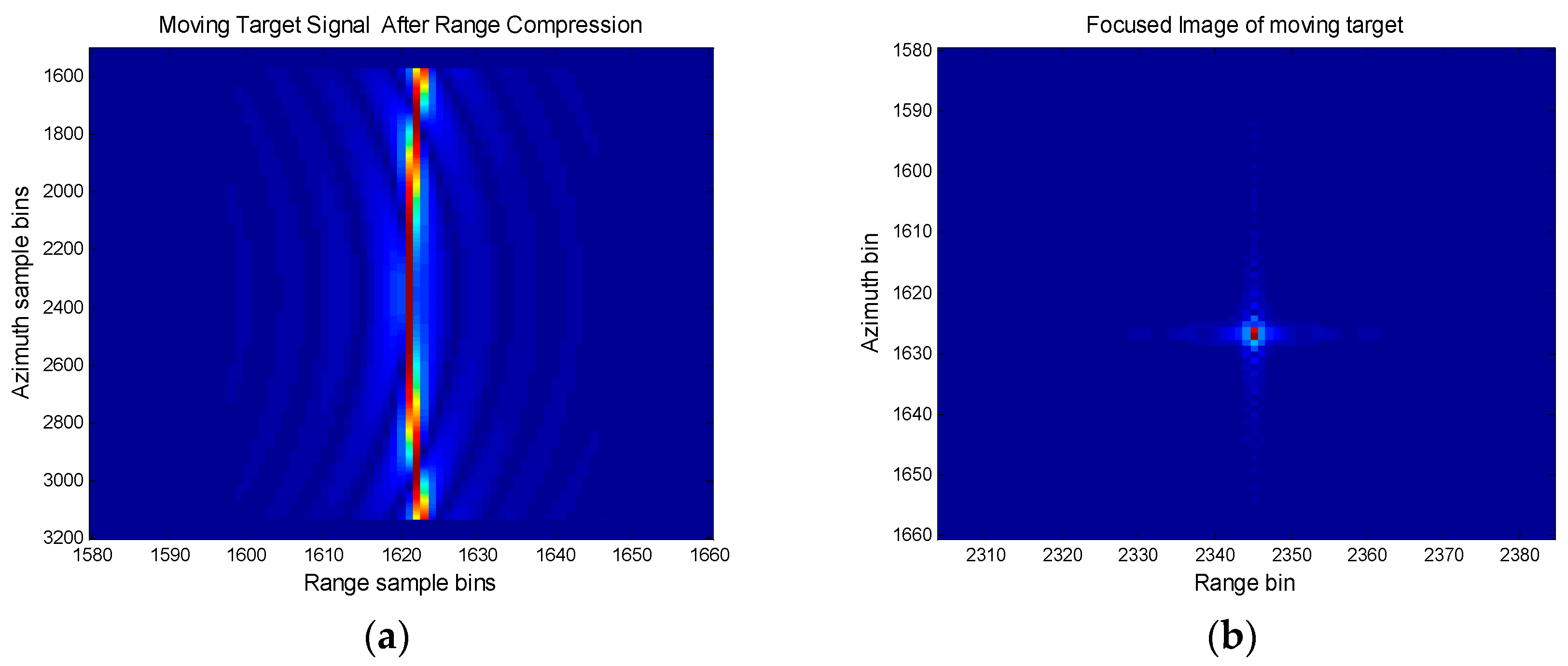
From the received signal of the m-th channel expressed in Equation (4), there exists a certain offset in the Doppler frequency compared to the signal of a static target. The frequency offset of each channel results in a frequency-dependent phase mismatch after the multichannel reconstruction introduced in Section 3.3. As a result, the phase mismatches among the channels will cause false targets along the azimuth when imaging. The phase error can be compensated after radial velocity estimation. After compensation for the phase errors, the traditional CS algorithm is applied to the imaging process. Figure 8a gives the trajectory of the moving target after range compression, where the linear RCM in Figure 5d is well corrected with the estimated radial velocity. Finally, the well-focused image of the moving target is obtained as shown in Figure 8b.
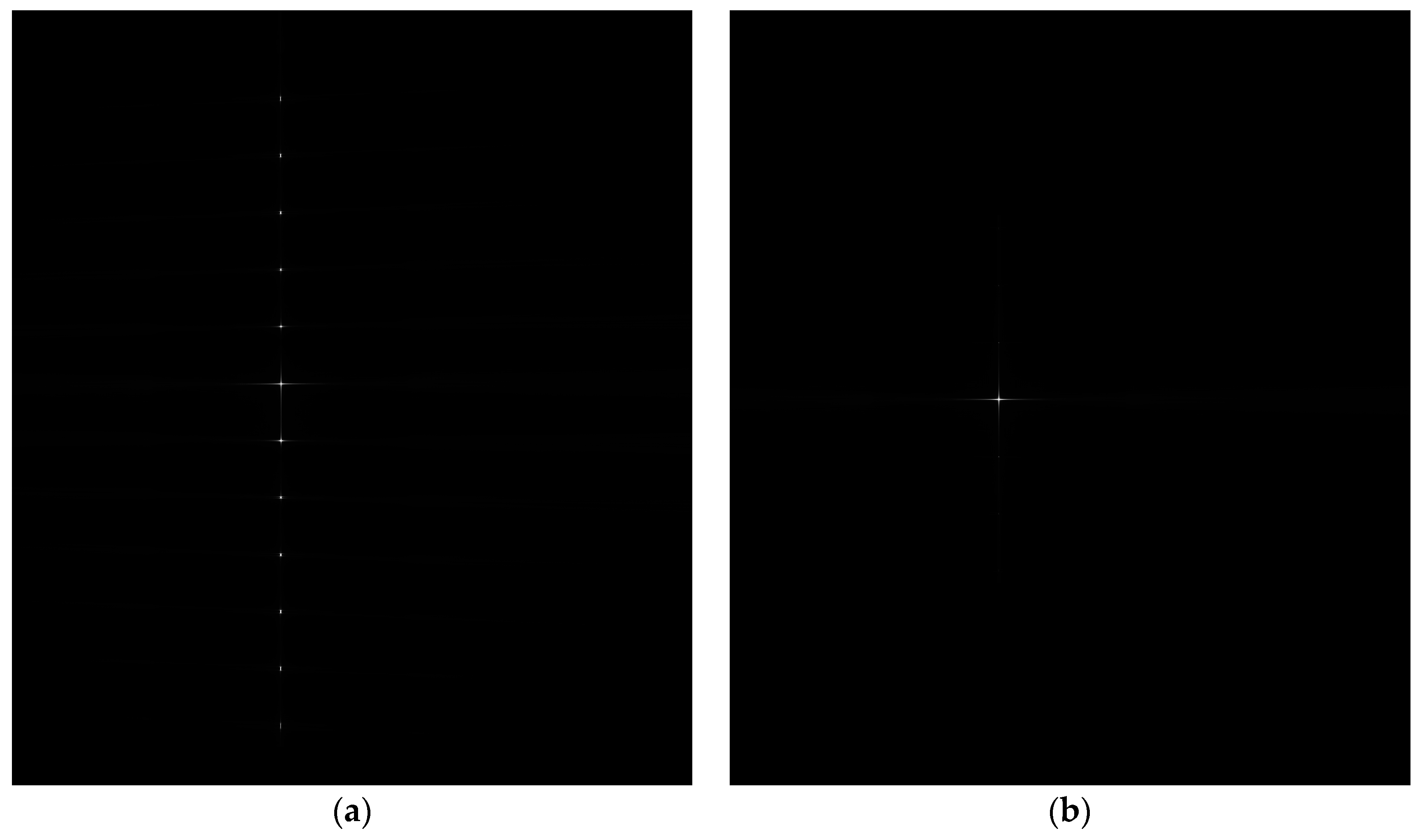
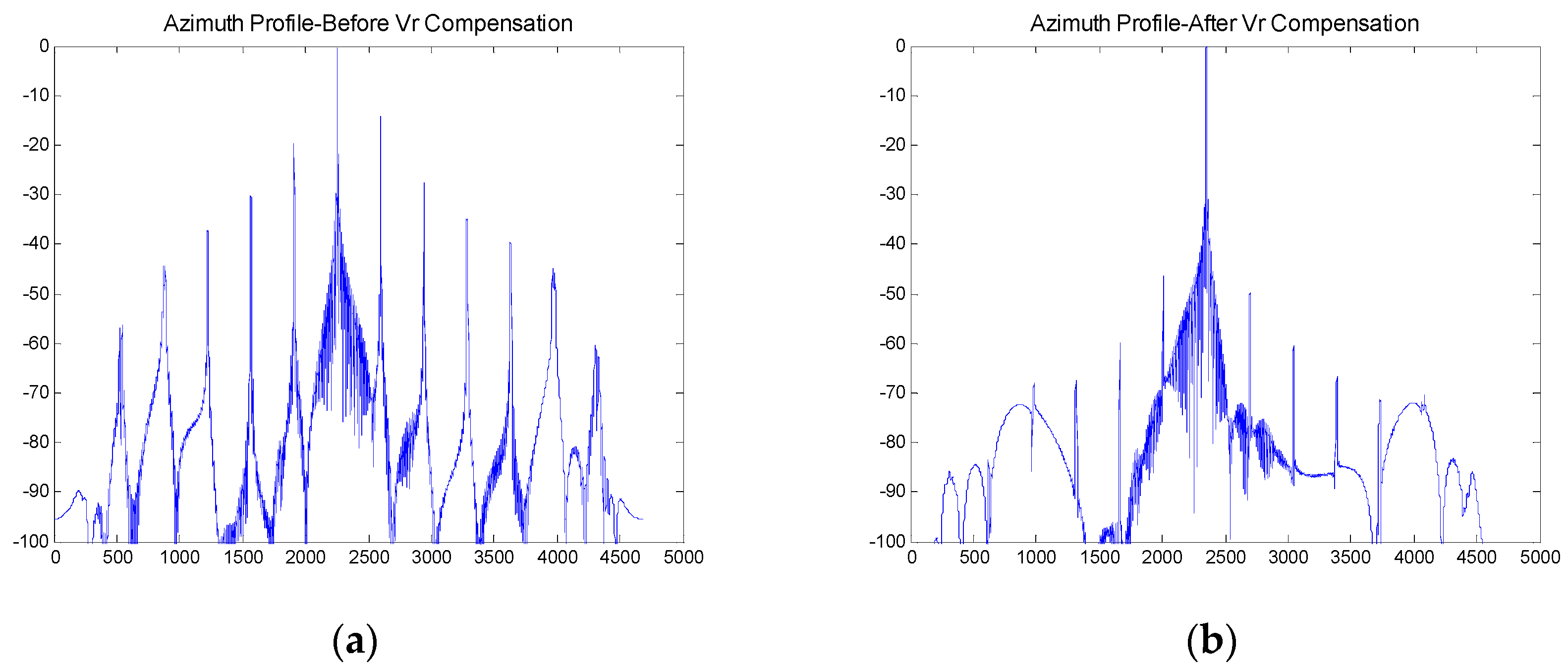
To demonstrate the impact of radial velocity on imaging quality for the multichannel SAR, we compare the imaging results before and after phase error compensation when the SNR = 0 dB in Figure 9. Figure 9a is the imagery of the moving target with traditional imaging process for multichannel SAR, where false targets are uniformly distributed along the azimuth around the real target. This is the impact of radial velocity on the multichannel SAR imaging. Figure 9b is the imagery after compensation for the phase offsets with the estimated velocity, where false targets are much suppressed and invisible. In Figure 10, the azimuth profiles of imaging results of the moving target are shown, Figure 10a corresponds to the azimuth profile of Figure 9a and Figure 10b corresponds to the azimuth profile of Figure 9b.
To quantifiably describe the impact of radial velocity, we compute the maximum power of false targets relative to the real one. The maximum power of false targets corresponding to Figure 9a is −13.49 dB. Table 3 summarizes the maximum powers after compensation for phase errors under different SNRs, which are smaller than −46.38 dB when the SNR is larger than 0 dB.
4.3. Estimation Accuracy under Clutter Interference
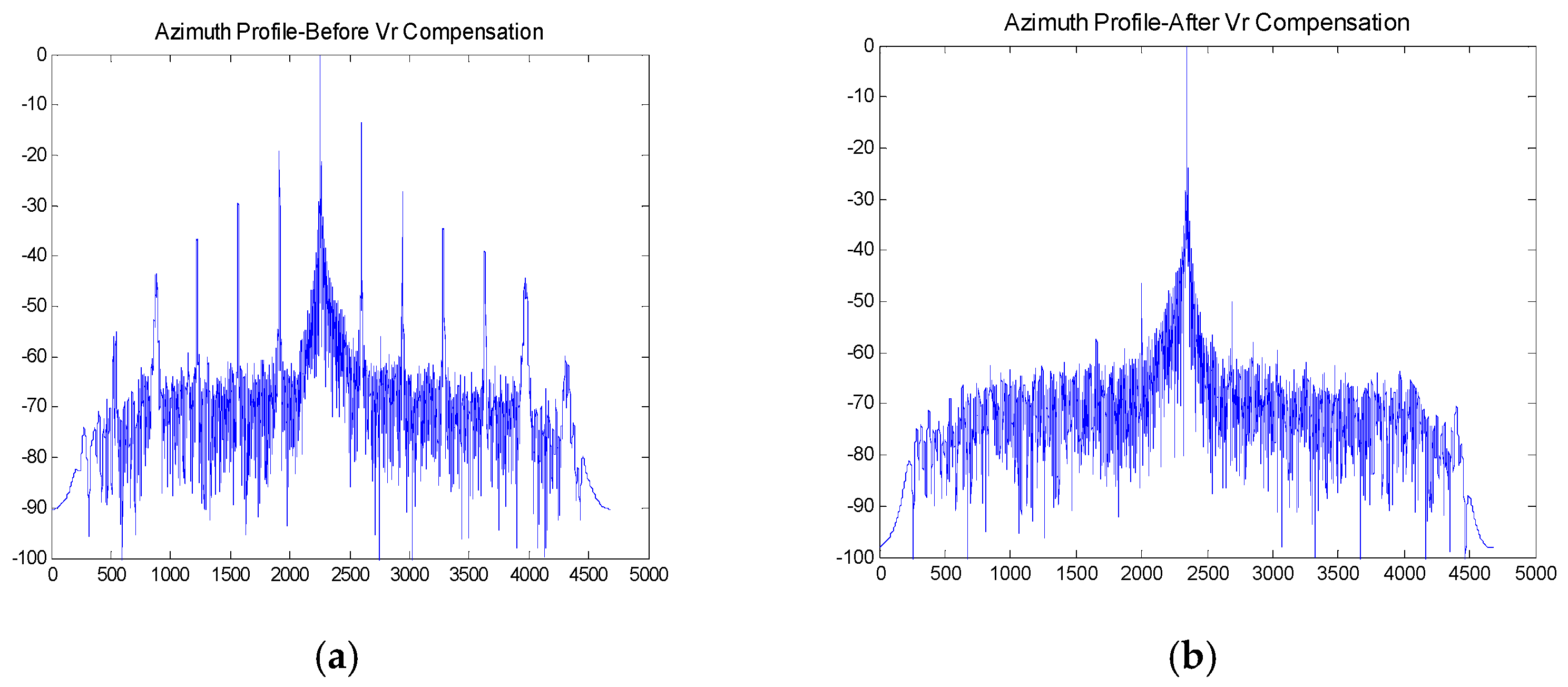
One of the primary applications of the spaceborne multichannel SAR system is the remote sensing of the sea surface, and sea clutter should be considered when detecting the moving ships. In the simulation, four commonly-used clutter models are simulated as the background of the detected scene. Rayleigh distribution is normally viewed as the magnitude probability function of the homogeneous scene. Weibull distribution, Log-normal distribution, and K-distribution are main magnitude models of the heterogeneous sea surfaces. The simulated clutter-interfered moving target signals are processed with the procedure in Section 3.3. In the simulation, the radial velocity of the moving target is 10 m/s, the signal-to-clutter ratio (SCR) is 0 dB and the SNR is 5 dB. The estimated radial velocities, the estimation errors and relative errors under different clutter distributions are listed in Table 4. Table 5 summarizes the maximum powers of false targets before and after compensation for estimated phase mismatches. We compare the imaging results before and after compensation under Weibull distribution clutter in Figure 11. In Figure 12, the azimuth profiles of imaging results are shown, Figure 12a corresponds to the azimuth profile of Figure 11a, and Figure 12b corresponds to the azimuth profile of Figure 11b.
5. Discussion
In Section 4, this paper conducted a comprehensive experiment to analyze the performance of the proposed ML-based radial velocity estimation algorithm. From the estimated value under different SNRs in Section 4.1, the relative estimation error is smaller than 2.2% when the SNR is larger than 0 dB. Thus this algorithm is accurate enough for applications. From the imaging results of the moving target in the clutter-free situation in Figure 9, the false targets are rather obvious along the azimuth with the traditional multichannel SAR imaging algorithm, and are visually unapparent after compensation for the azimuth offsets with the estimated radial velocity. The maximum power of false targets after compensation has been suppressed by more than 30 dB.
When the moving target is interfered by the sea clutter, the proposed algorithm can still estimate the radial velocity. However, the performance is poorer than the ideal condition. Considering different sea clutter distributions with SCR = 0 dB and SNR = 5 dB, the relative estimation error is at least 3.3%, compared to that of 0.8% without clutter. Figure 11 demonstrates that the ML-based algorithm can also estimate velocity and suppress false targets even in the interference of strong sea clutters. Despite the maximum power of false targets with sea clutter interference being larger than that without clutter, the deterioration of the performance is tolerable. Combined with Figure 9 and Figure 11, the applicability of the proposed estimation algorithm under different practical conditions is verified.
In terms of the estimation effectiveness, we have verified it in Figure 7, where the RMSE infinitely approaches the CRLB with the increase of the SNR. As for the computational complexity, this algorithm does not require iteration or matrix Eigen-decomposition, thus the computational load only lies in the searching process of radial velocity. Finally, we have demonstrated that the proposed algorithm can obtain accurate, efficient, and real-time estimation of the velocity of moving targets for HRWS SAR systems.
6. Conclusions
A novel algorithm is proposed to estimate the velocity of the moving target for the spaceborne HRWS SAR system. The main impact of the radial velocity is an additional Doppler spectrum shift in the echo of each channel compared to that of the static target, leading to false targets along the azimuth. According to the characteristics of a moving target signal, a maximum likelihood based algorithm is proposed to estimate the sparse cone angle of the target, obtaining the radial velocity indirectly. Moreover, for the peculiarity of the multichannel SAR system, the Doppler ambiguity is considered in the estimation. After velocity estimation, the multichannel echoes are reconstructed and phase mismatches are compensated to obtain the fine and unambiguous SAR image. The experimental results show high accuracy of the proposed method even under different sea clutter distributions. The effectiveness of the algorithm is also verified by comparing the RMSE and the CRLB. The proposed algorithm can precisely estimate the moving target’s velocity for the special mode of HRWS SAR system, providing a reference for applications in remote sensing of the sea surface in future spaceborne multichannel SAR systems.
Acknowledgments
This work was jointly supported by the National Science Foundation of China under Grant No. 61331017.
Author Contributions
Tingting Jin, Xiaolan Qiu, Donghui Hu and Chibiao Ding initiated the research. Under supervision of Xiaolan Qiu, Tingting Jin performed the experiments and analysis. Tingting Jin wrote the manuscript, and Xiaolan Qiu and Donghui Hu revised the manuscript. All authors read and approved the final version of the manuscript.
Conflicts of Interest
The authors declare no conflict of interest.
References
- Gebert, N.; Krieger, G.; Moreira, A. Digital beamforming on receive: Techniques and optimization strategies for high-resolution wideswath SAR imaging. IEEE Trans. Aerosp. Electron. Syst. 2009, 45, 564–592. [Google Scholar] [CrossRef]
- Baumgartner, S.V.; Krieger, G. Simultaneous high-resolution wide-swath SAR imaging and ground moving target indication: Processing approaches and system concepts. IEEE J. Sel. Top. Appl. Earth Obs. Remote Sens. 2016, 8, 1–13. [Google Scholar] [CrossRef]
- Suchandt, S.; Runge, H.; Steinbrecher, U. Ship detection and measurement using the TerraSAR-X dual-receive antenna mode. In Proceedings of the 2010 IEEE International Geoscience and Remote Sensing Symposium (IGARSS), Honolulu, HI, USA, 25–30 July 2010; pp. 2860–2863. [Google Scholar]
- Rosenqvist, A.; Shimada, M.; Suzuki, S.; Ohgushi, F.; Tadono, T.; Watanabe, M.; Tsuzuku, K.; Watanabe, T.; Kamijo, S.; Aoki, E. Operational performance of the ALOS global systematic acquisition strategy and observation plans for ALOS-2 PALSAR-2. Remote Sens. Environ. 2014, 155, 3–12. [Google Scholar] [CrossRef]
- Dragosevic, M.V.; Burwash, W.; Shen, C. Detection and estimation with RADARSAT-2 moving-object detection experiment modes. IEEE Trans. Geosci. Remote Sens. 2012, 50, 3527–3543. [Google Scholar] [CrossRef]
- Gao, R.; Shi, G.T.; Yang, L.; Zhou, S.L. Moving target detection based on the spreading characteristics of SAR interferograms in the magnitude-phase plane. Remote Sens. 2015, 7, 1836–1854. [Google Scholar] [CrossRef]
- Sikaneta, I.C.; Chouinard, J.Y. Eigen-decomposition of the multi-channel covariance matrix with applications to SAR-GMTI. Signal Process. 2004, 84, 1501–1535. [Google Scholar] [CrossRef]
- Yang, T.L.; Wang, Y. A novel algorithm to estimate moving target velocity for a spaceborne HRWS SAR/GMTI system. In Proceedings of the 2010 IEEE International Geoscience and Remote Sensing Symposium (IGARSS), Beijing, China, 10–15 July 2016; pp. 3242–3245. [Google Scholar]
- Baumgartner, S.V.; Krieger, G. Experimental verification of high-resolution wide-swath moving target indication. In Proceedings of the 11th European Conference on Synthetic Aperture Radar (EUSAR), Hamburg, Germany, 6–9 June 2016; pp. 1265–1270. [Google Scholar]
- Wang, X.Y.; Wang, R.; Li, N.; Zhou, C. A velocity estimation method of moving target for HRWS SAR. In Proceedings of the 2010 IEEE International Geoscience and Remote Sensing Symposium (IGARSS), Beijing, China, 10–15 July 2016; pp. 6819–6822. [Google Scholar]
- Zhang, S.X.; Xing, M.D.; Xia, X.G.; Guo, R.; Liu, Y.Y.; Bao, Z. A novel moving target imaging algorithm for HRWS SAR based on local maximum-likelihood minimum entropy. IEEE Trans. Geosci. Remote Sens. 2014, 52, 5333–5348. [Google Scholar] [CrossRef]
- Wu, Q.; Xing, M.; Qiu, C.; Liu, H.W. Motion parameter estimation in the SAR system with low PRF sampling. IEEE Geosci. Remote Sens. Lett. 2010, 7, 540–544. [Google Scholar] [CrossRef]
- Yang, T.; Li, Z.; Suo, Z.; Bao, Z. Ground moving target indication for high-resolution wide-swath synthetic aperture radar systems. IET Radar Sonar Navig. 2014, 8, 227–232. [Google Scholar] [CrossRef]
- Wang, L.B.; Wang, D.W.; Li, J.J.; Xu, J.; Xie, C.; Wang, L. Ground moving target detection and imaging using a virtual multichannel scheme in HRWS mode. IEEE Trans. Geosci. Remote Sens. 2016, 54, 1–16. [Google Scholar] [CrossRef]
- Zhang, S.X.; Xing, M.D.; Xia, X.G.; Guo, R.; Liu, Y.Y.; Bao, Z. Robust clutter suppression and moving target imaging approach for multichannel in azimuth high-resolution and wide-swath synthetic aperture radar. IEEE Trans. Geosci. Remote Sens. 2015, 53, 687–709. [Google Scholar] [CrossRef]
- Malioutov, D.C.; Etin, M.; Willsky, A.S. A sparse signal reconstruction perspective for source localization with sensor arrays. IEEE Trans. Signal Process. 2005, 53, 3010–3022. [Google Scholar] [CrossRef]
- Gabele, M.; Krieger, G. Moving target signals in high resolution wide swath SAR. In Proceedings of the 9th European Conference on Synthetic Aperture Radar (EUSAR), Friedrichshafen, Germany, 2–5 June 2008; pp. 1–4. [Google Scholar]
- Satish, A.; Kashyap, R.L. Maximum likelihood estimation and cramer-rao bounds for direction of arrival parameters with a large sensor array. IEEE Trans. Geosci. Remote Sens. 1996, 44, 478–491. [Google Scholar] [CrossRef]
- Tam, P.K.; Wong, K.T.; Song, Y. An hybrid Cramér-Rao bound in closed form for direction-of-arrival estimation by an “acoustic vector sensor” with gain-phase uncertainties. IEEE Trans. Signal Process. 2014, 62, 2504–2516. [Google Scholar] [CrossRef]
- Stoica, P.; Nehorai, A. Performance study of conditional and unconditional direction-of-arrival estimation. IEEE Trans. Acoust. Speech Signal Process. 1990, 38, 1783–1795. [Google Scholar] [CrossRef]
Figure 1.
The imaging geometry of the high-resolution and wide-swath (HRWS) synthetic aperture radar (SAR) system.
Figure 1.
The imaging geometry of the high-resolution and wide-swath (HRWS) synthetic aperture radar (SAR) system.
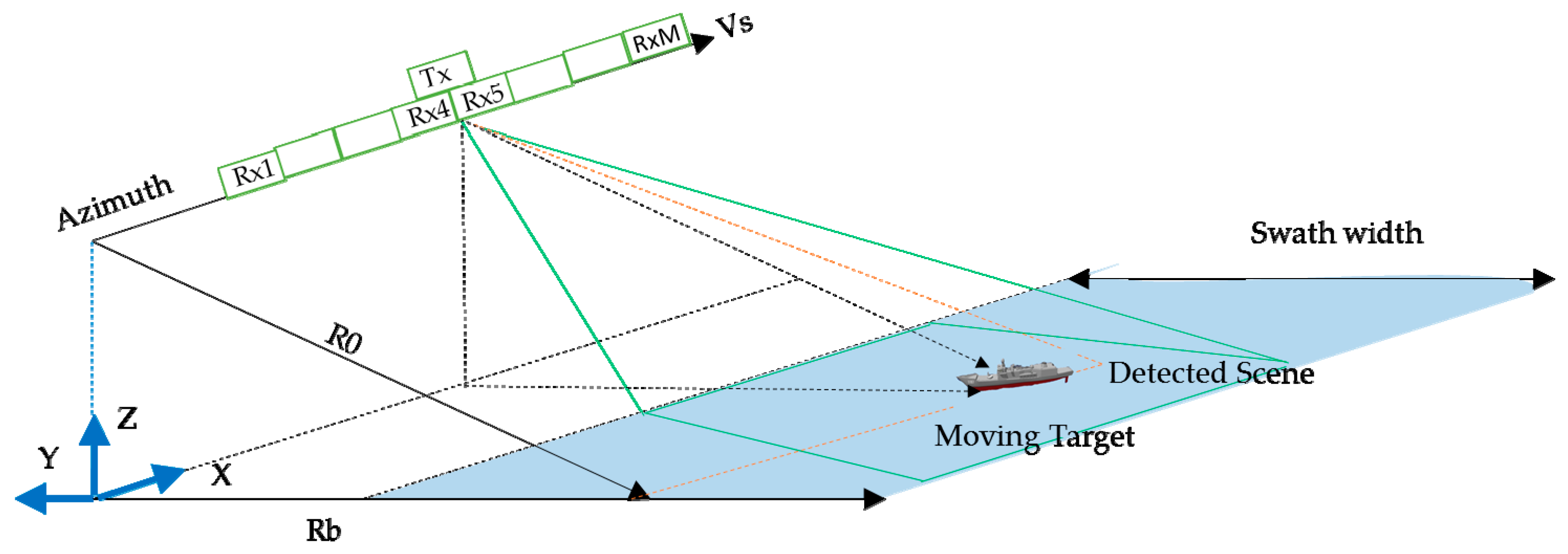
Figure 2.
Spatial-temporal spectra of echoes: (a) unambiguous; and (b) Doppler ambiguous.
Figure 3.
Processing flow of the moving target for the HRWS SAR system.

Figure 4.
Diagram of the transmitting and receiving centers.
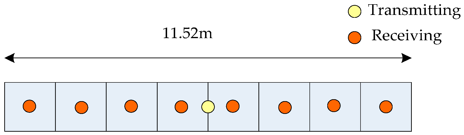
Figure 5.
Comparison of the Doppler spectra and Range-compressed signals between clutter and the moving target: (a) Doppler spectrum of the clutter signal; (b) Doppler spectrum of the moving target; (c) range-compressed signal of the clutter signal; and (d) range-compressed signal of the moving target.

Figure 6.
Maximum likelihood spectrum of radial velocity.

Figure 7.
Root mean squired error (RMSE) versus Cramér–Rao lower bound (CRLB) of radial velocity estimation.
Figure 7.
Root mean squired error (RMSE) versus Cramér–Rao lower bound (CRLB) of radial velocity estimation.
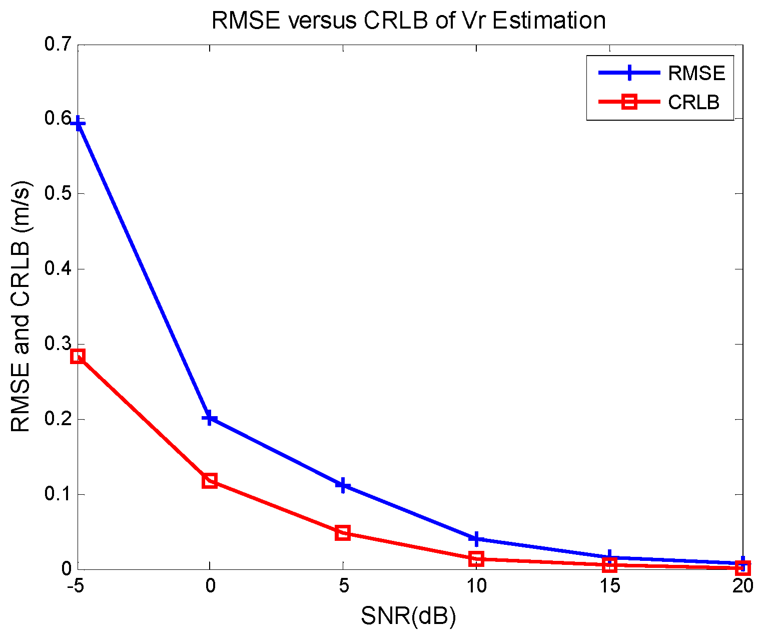
Figure 8.
Imaging process after compensation for the errors caused by target motion: (a) Trajectory of the moving target after range compression; and (b) focused image of the moving target.
Figure 8.
Imaging process after compensation for the errors caused by target motion: (a) Trajectory of the moving target after range compression; and (b) focused image of the moving target.

Figure 9.
Imaging results before and after compensation for the errors caused by target motion: (a) before compensation; and (b) after compensation.
Figure 9.
Imaging results before and after compensation for the errors caused by target motion: (a) before compensation; and (b) after compensation.

Figure 10.
Azimuth profile of imaging result of the moving target: (a) before compensation; (b) after compensation.
Figure 10.
Azimuth profile of imaging result of the moving target: (a) before compensation; (b) after compensation.

Figure 11.
Imaging results before and after compensation under Weibull clutter: (a) before compensation; and (b) after compensation.
Figure 11.
Imaging results before and after compensation under Weibull clutter: (a) before compensation; and (b) after compensation.
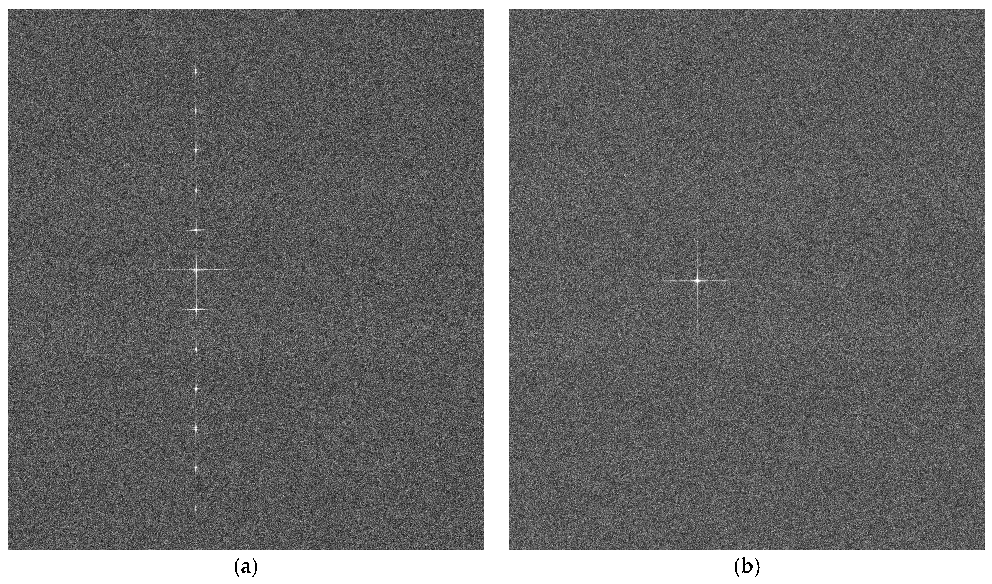
Figure 12.
Azimuth profile of imaging result of the moving target under Weibull clutter: (a) before compensation; and (b) after compensation.
Figure 12.
Azimuth profile of imaging result of the moving target under Weibull clutter: (a) before compensation; and (b) after compensation.


Table 1.
Parameters of the simulated spaceborne multichannel SAR system.
| Parameter | Symbol | Value |
|---|---|---|
| Number of Channels | M | 8 |
| Aperture Size | Da | 11.2 m |
| Wavelength | 0.05556 m | |
| Look Angle | 53.45 degrees | |
| PRF | 1317.1 Hz | |
| Doppler Bandwidth | 5987.9 Hz | |
| Satellite Velocity | 7586.5 m/s | |
| Sample Frequency | 80 MHz | |
| Bandwidth | 67 MHz | |
| Pulsewidth | 38 |
Table 2.
Estimated Radial Velocities and Errors under different signal-to-noise ratios (SNRs).
| SNR (dB) | −5 | 0 | 5 | 10 | 15 | 20 |
|---|---|---|---|---|---|---|
| Estimated Value (m/s) | 10.47 | 10.22 | 10.08 | 9.97 | 9.99 | 10.00 |
| Estimation Error (m/s) | 0.47 | 0.22 | 0.08 | 0.03 | 0.01 | 0 |
| Relative Error | 4.7% | 2.2% | 0.8% | 0.3% | 0.1% | 0 |
Table 3.
The maximum power of false targets.
| SNR (dB) | −5 | 0 | 5 | 10 | 15 | 20 |
| Maximum Power (dB) | −40.48 | −46.38 | −52.92 | −55.08 | −55.23 | −58.59 |
Table 4.
Estimated radial velocities and errors under different clutter distributions.
| Clutter Distribution | Rayleigh Distribution | Weibull Distribution | Log-Normal Distribution | K-Distribution |
|---|---|---|---|---|
| Estimated Value (m/s) | 10.33 | 10.57 | 10.38 | 10.37 |
| Estimation Error (m/s) | 0.33 | 0.57 | 0.38 | 0.37 |
| Relative Error | 3.3% | 5.7% | 3.8% | 3.7% |
Table 5.
The maximum power of false targets under different clutter distributions.
| Clutter Distribution | Rayleigh Distribution | Weibull Distribution | Log-Normal Distribution | K-Distribution |
|---|---|---|---|---|
| Before Compensation (dB) | −13.49 | −13.50 | −13.47 | −13.50 |
| After Compensation (dB) | −46.46 | −42.30 | −43.57 | −45.35 |
© 2017 by the authors. Licensee MDPI, Basel, Switzerland. This article is an open access article distributed under the terms and conditions of the Creative Commons Attribution (CC BY) license (http://creativecommons.org/licenses/by/4.0/).
Share and Cite
MDPI and ACS Style
Jin, T.; Qiu, X.; Hu, D.; Ding, C. An ML-Based Radial Velocity Estimation Algorithm for Moving Targets in Spaceborne High-Resolution and Wide-Swath SAR Systems. Remote Sens. 2017, 9, 404. https://doi.org/10.3390/rs9050404
AMA Style
Jin T, Qiu X, Hu D, Ding C. An ML-Based Radial Velocity Estimation Algorithm for Moving Targets in Spaceborne High-Resolution and Wide-Swath SAR Systems. Remote Sensing. 2017; 9(5):404. https://doi.org/10.3390/rs9050404
Chicago/Turabian StyleJin, Tingting, Xiaolan Qiu, Donghui Hu, and Chibiao Ding. 2017. "An ML-Based Radial Velocity Estimation Algorithm for Moving Targets in Spaceborne High-Resolution and Wide-Swath SAR Systems" Remote Sensing 9, no. 5: 404. https://doi.org/10.3390/rs9050404
Note that from the first issue of 2016, this journal uses article numbers instead of page numbers. See further details here.