
Terrestrial Hyperspectral Image Shadow Restoration through Lidar Fusion


1
Department of Civil and Environmental Engineering, University of Houston, 4726 Calhoun Rd., Houston, TX 77204, USA
2
Department of Earth and Atmospheric Sciences, University of Houston, 3507 Cullen Blvd., Houston, TX 77204, USA
*
Author to whom correspondence should be addressed.
Remote Sens. 2017, 9(5), 421; https://doi.org/10.3390/rs9050421
Submission received: 2 March 2017
/
Revised: 20 April 2017
/
Accepted: 27 April 2017
/
Published: 29 April 2017
Abstract
:Acquisition of hyperspectral imagery (HSI) from cameras mounted on terrestrial platforms is a relatively recent development that enables spectral analysis of dominantly vertical structures. Although solar shadowing is prevalent in terrestrial HSI due to the vertical scene geometry, automated shadow detection and restoration algorithms have not yet been applied to this capture modality. We investigate the fusion of terrestrial laser scanning (TLS) spatial information with terrestrial HSI for geometric shadow detection on a rough vertical surface and examine the contribution of radiometrically calibrated TLS intensity, which is resistant to the influence of solar shadowing, to HSI shadow restoration. Qualitative assessment of the shadow detection results indicates pixel level accuracy, which is indirectly validated by shadow restoration improvements when sub-pixel shadow detection is used in lieu of single pixel detection. The inclusion of TLS intensity in existing shadow restoration algorithms that use regions of matching material in sun and shade exposures was found to have a marginal positive influence on restoring shadow spectrum shape, while a proposed combination of TLS intensity with passive HSI spectra boosts restored shadow spectrum magnitude precision by 40% and band correlation with respect to a truth image by 45% compared to existing restoration methods.
1. Introduction
The standard method for remotely sensing topographic features with high spectral and spatial resolution is passive hyperspectral imaging (HSI). HSI data are characterized by hundreds of spectrally narrow (5–10 nm) and contiguous bands in the visible to shortwave infrared (~380–2500 nm) portion of the electromagnetic spectrum [1]. Since their development three decades ago [2], HSI sensors have traditionally been deployed from aircraft in nadir viewing geometry, e.g., the Airborne Visible/Infrared Imaging Spectrometer (AVIRIS) developed by the Jet Propulsion Laboratory and similar commercial systems. Deployment of HSI cameras from terrestrial platforms for Earth remote sensing has only emerged in the past decade, and is often fused with dense lidar (light detection and ranging) point cloud data acquired with terrestrial laser scanning (TLS) instruments to create 3D models of predominantly vertical scenes containing rich structural and spectral information [3,4].
The majority of literature dealing with fused TLS and HSI information is geologic in application. Examples include digital outcrop modeling for hydrocarbon reservoir analog creation [3,4,5] and open pit mine face modeling for quantitative mineral content analysis [6,7,8]. The inclusion of high resolution spectral information in these applications has the potential to enhance automatic identification of outcrop lithology through a variety of standard image processing and classification techniques [5,6,7,8,9] as well as expert systems that identify unique electronic and vibrational spectral absorption features only detectable with HSI [10,11]. For sufficiently curved outcrops, the exposed linear interfaces between spectrally identified lithologies can also be used to create planar surfaces extending into the outcrop interior for 3D volumetric analyses [12], such as for geocellular reservoir modeling for simulating hydrocarbon fluid flow [13].
Given the dominantly vertical and geometrically rugged nature of geologic outcrop formations, terrestrial HSI often contains a high proportion of shadowed pixels, even when collected during optimal sunlight conditions. Unless restored to sunlit conditions, shadows can reduce the amount of HSI information, i.e., shadowed areas need to be masked out [4], or reduce the effectiveness of the HSI for material identification by deteriorating classification or target identification accuracy [9,10,11,12,13,14]. Numerous studies have examined shadow restoration in airborne HSI (e.g., see [15,16,17]), but the topic has yet to be addressed for HSI captured from a terrestrial modality. This may be due in part to the relatively recent emergence of terrestrial HSI as well as the development of radiative transfer models for application to HSI collected from nadir-looking airborne HSI sensors, e.g., FLAASH [18] and ATCOR [19], rather than HSI collected with horizontally viewing sensors.
This paper examines shadow detection and restoration techniques in terrestrially acquired short wave infrared (SWIR) HSI of a vertical outcrop, which was imaged in maximum sun, partial sun, and full shade conditions to enable comparison of restored shadow pixel spectra to their full sun counterparts. The HSI was fused with TLS point cloud data in order to detect shadowed HSI pixels via geometric ray tracing and to examine the influence of the backscattered laser energy, i.e., lidar intensity, on the identification of regions of matching material in sunlit and shadowed areas, which underpins many existing shadow restoration methods. A direct combination of radiometrically calibrated lidar intensity with the HSI pixel spectra for shadow restoration was also investigated, and the impact of multispectral lidar on this technique simulated. Qualitative assessment of the shadow detection results indicates pixel level accuracy, which is indirectly validated by shadow restoration improvements when moving from single pixel to sub-pixel shadow detection. The inclusion of TLS intensity information in existing shadow restoration algorithms was found to have a marginal positive influence on improving HSI shadow restoration techniques employing matching material regions. However, the proposed direct combination of TLS intensity with passive HSI spectra boosted the precision of restored shadow spectrum magnitudes by 40% and band correlation with respect to a truth image by 45% compared to the matching material restoration methods. Finally, simulation of multispectral lidar intensity directly applied to HSI shadow restoration found that as few as 8–10 wavelengths are required for a computationally efficient method of restoring shadowed HSI pixel spectra.
2. Data Description
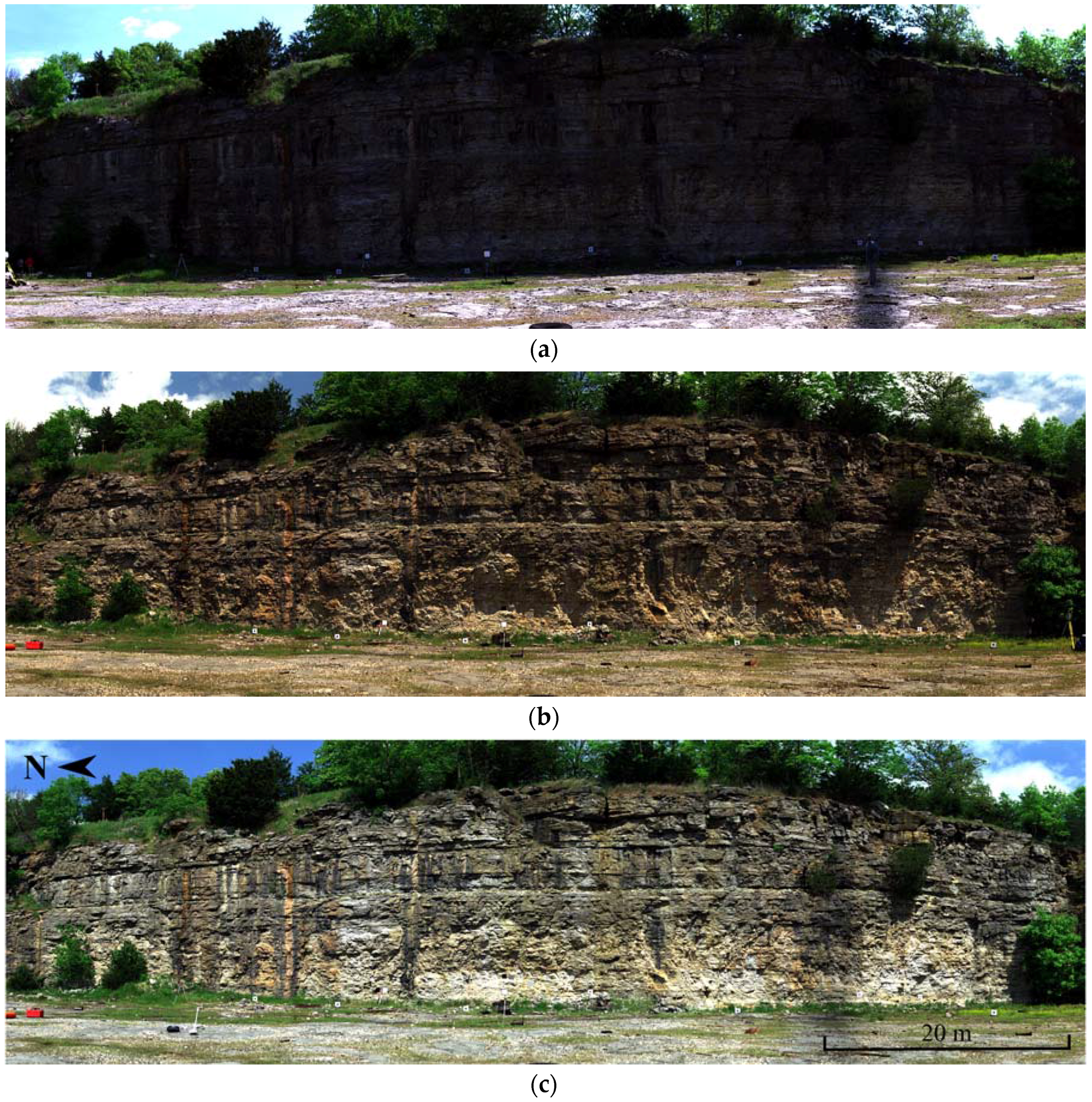
TLS and HSI measurements of the east wall of an abandoned quarry located near Huntsville, Arkansas were acquired on 4 May 2015. The site was chosen for analysis because of the ability to capture HSI of the wall in full shade, partial sun, and maximum sun exposures (see Figure 1), which enables validation of the HSI shadow restoration. The quarry floor and vegetation on the top of the wall were cropped from the TLS and HSI products in order to limit the analysis to the vertical rock surface. Although both SWIR (970–2500 nm) and visible to near infrared (VNIR, 400–1000 nm) HSI was collected, only the SWIR data are analyzed in this paper for brevity. The VNIR results are similar, but the spectral shapes are relatively flat with few absorption features and thus potentially less applicable for geologic studies.
2.1. TLS
A 1550 nm laser wavelength Riegl VZ-400 TLS (see Table 1) collected data at three scan positions, each offset approximately 16 m from the outcrop face. Point spacing was set to less than 5 mm at a nominal distance of 16 m and the point clouds were co-registered using the multi-station adjustment routine within Riegl’s RiSCAN PRO desktop software to within ±2.5 mm at 1σ. The co-registered point clouds were georeferenced to the WGS84 (G1762) datum using post-processed static GNSS observations collected with antennas mounted on top of four retroreflective cylinder targets surrounding the project area. The point cloud was then transformed to a local geodetic coordinate system centered at the base of the quarry wall in order to support shadow computations that utilize local solar zenith and azimuth angles. TLS point intensities were converted to reflectance using empirical observations of Spectralon panels of multiple reflectance values at multiple ranges; see [20] for an explanation of the method.
A triangulated mesh was created from the point cloud to serve as the basis for occlusion analysis to determine shadow locations in the HSI and the visibility of each TLS point to the HSI camera. In order to accommodate the roughness and curvature of the outcrop, the mesh surface reconstruction algorithm developed by [21], as implemented in the open source CloudCompare point cloud software [22], was used to create a fully 3D mesh that follows the complex, undulating surface sampled by the TLS points.
2.2. HSI
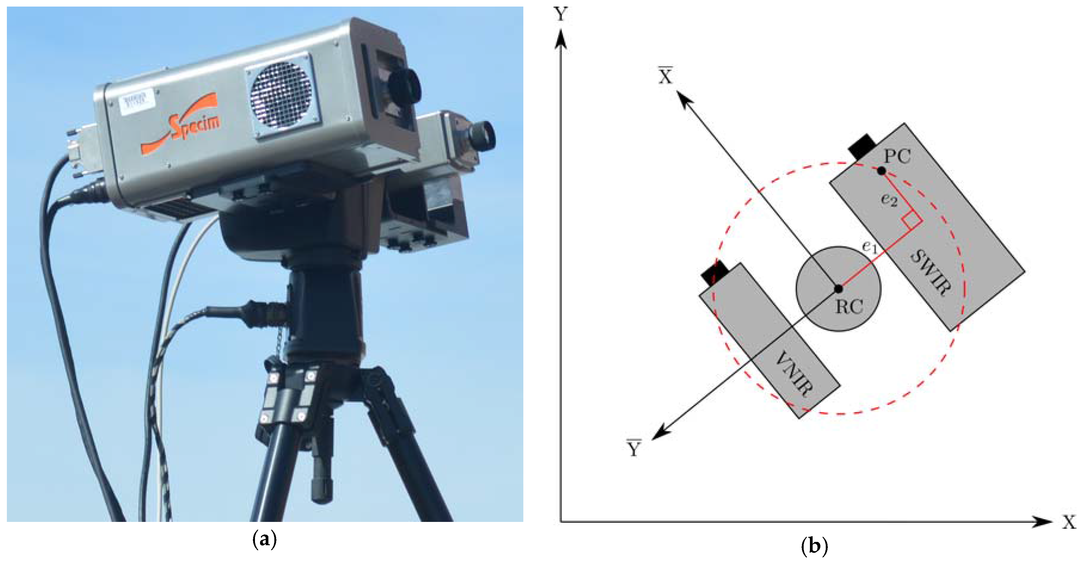
Images were collected with a SWIR camera manufactured by Spectral Imaging, Ltd. (see Table 1) in the morning, mid-day, and afternoon to capture the wall in full shade, partial shade, and maximum sun conditions. These images will be referred to as SWIR-shade, SWIR-partial, and SWIR-sun hereafter. The camera was positioned 41 m from the east quarry wall at approximately the same location for each image acquisition, which equates to a minimum pixel size of 55 mm. The camera was mounted on a rotating stage (Figure 2a) with the rotation and camera exposure rates selected to produce approximately square pixels. Dark current was removed from the HSI by subtracting the mean of 100 camera exposures collected with the lens cap installed on the camera. Abnormal pixels causing linear image artifacts were detected and replaced following the method in [23], which uses the mean of the two immediately adjacent lines for the correction. Wavelengths subject to strong atmospheric water and carbon dioxide absorption (1334–1460 nm and 1788–1958 nm) were removed from the HSI along with wavelengths at the camera spectrum extremities (896–922 nm and 2447–2504 nm) due to high noise. The empirical line method was applied to convert the HSI units from digital numbers (DNs) to relative reflectance using pixels that captured 99% and 2% reflectivity Spectralon panels that were placed at the base of the outcrop.
2.3. TLS and HSI Fusion
2.3.1. Camera Model
The fusion of TLS spatial and spectral information with the HSI, as well as HSI pixel shadow determination, relies on a calibrated camera model defining the geometric relationship between 3D object space and the 2D HSI image space. The model allows 3D object space points to be projected into image space and the inverse of this operation, i.e., the creation of 3D object space rays emanating from the camera, for any desired image pixel. To date, most of the terrestrial HSI applied to geologic studies has been collected with panoramic linear array sensors that rotate around a vertical axis intersecting the camera optical centerline, thus forming a standard cylindrical model [5,24]. However, the optical centerline of the SWIR camera used in this work is offset from the stage rotation axis by approximately 20 cm due to the simultaneous presence of both the VNIR and SWIR cameras on the stage (see Figure 2). Furthermore, the camera vertical inclination can be adjusted prior to horizontal rotation in order to maximize coverage of vertical structures at close proximity. Therefore, a camera model similar to that found in [25], where the offset optical axis is explicitly accommodated, was used. The standard offset panoramic camera model was augmented to include the camera vertical inclination angle and parameters were added to handle camera tilt about the optical axis, pixel affinity (non-square pixels), and radial lens distortion. A brief description of the camera model and its role in the fusion process is described in the following paragraphs; see [26] for a complete mathematical derivation of the camera model.
In order to fuse, i.e., register, the HSI with TLS point or mesh data, the exterior orientation (EO) and interior orientation (IO) of the camera must be solved. The EO refers to the position and orientation of the camera coordinate system relative to the object space, i.e., world, coordinate system. This is defined by a rigid body transformation consisting of three rotation angles about the object space axes and three translation values. The IO refers to the geometry of the camera within the camera coordinate system that influences the pixel location of a ray of light passing through the lens into the camera. The IO is parameterized by the camera vertical inclination angle with respect to the disk swept by the camera projection center as it rotates, the location of the camera projection center relative to the stage rotation axis (described by the orthogonal distance from the stage rotation axis to the camera optical centerline () and the distance from the camera projection center to the point of intersection on the optical centerline (), (see Figure 2b)), the camera lens focal length and radial distortion terms (), the tilt of the camera about the optical centerline, and pixel affinity. A series of equations utilizing these parameters is then used transform a 3D object space location, i.e., a TLS point, into image space pixel coordinates. This link between TLS object space points and HSI image space pixels represents the fusion between the two remote sensing methods. Note that the math model can also be inverted to project a 3D ray from an image space pixel location into object space.
Four of the camera IO parameters are independent of image acquisition () and can be fixed after recovering their values in a least squares based resection adjustment. Toward this end, matching object and image space coordinates were extracted from a TLS point cloud and HSI that captured an array of synthetic targets placed at various angles and distances from the instruments. The target coordinates were inserted into the least squares resection algorithm and all EO and IO parameters simultaneously solved by minimizing the distances between the measured HSI target pixel coordinates and the corresponding pixel coordinates generated by projecting the 3D object space target coordinates into image space via the math model. Using simple manual point selection in both the TLS point cloud and HSI image to generate the required coordinates, normally distributed residuals with a sub-pixel standard deviation were produced (Figure 3). By reducing the number of unknown IO parameters, subsequent HSI and TLS fusion tasks require selection of fewer common image and object space points for the least squares adjustment since there are fewer unknowns to be solved.
2.3.2. HSI Registration
With the camera model defined and several IO parameters calibrated and fixed, the remaining unknown camera IO and EO parameters were solved for each of the HSI images: SWIR-shade, SWIR-partial, and SWIR-sun. A combination of synthetic signalized targets at the outcrop base and manually identified natural features in the middle and top of the outcrop were selected from the TLS point cloud and each HSI image for input into the least squares resection adjustment algorithm.
Similar to the results for the calibration of the fixed IO parameters, sub-pixel residual standard deviations were achieved for each adjustment.
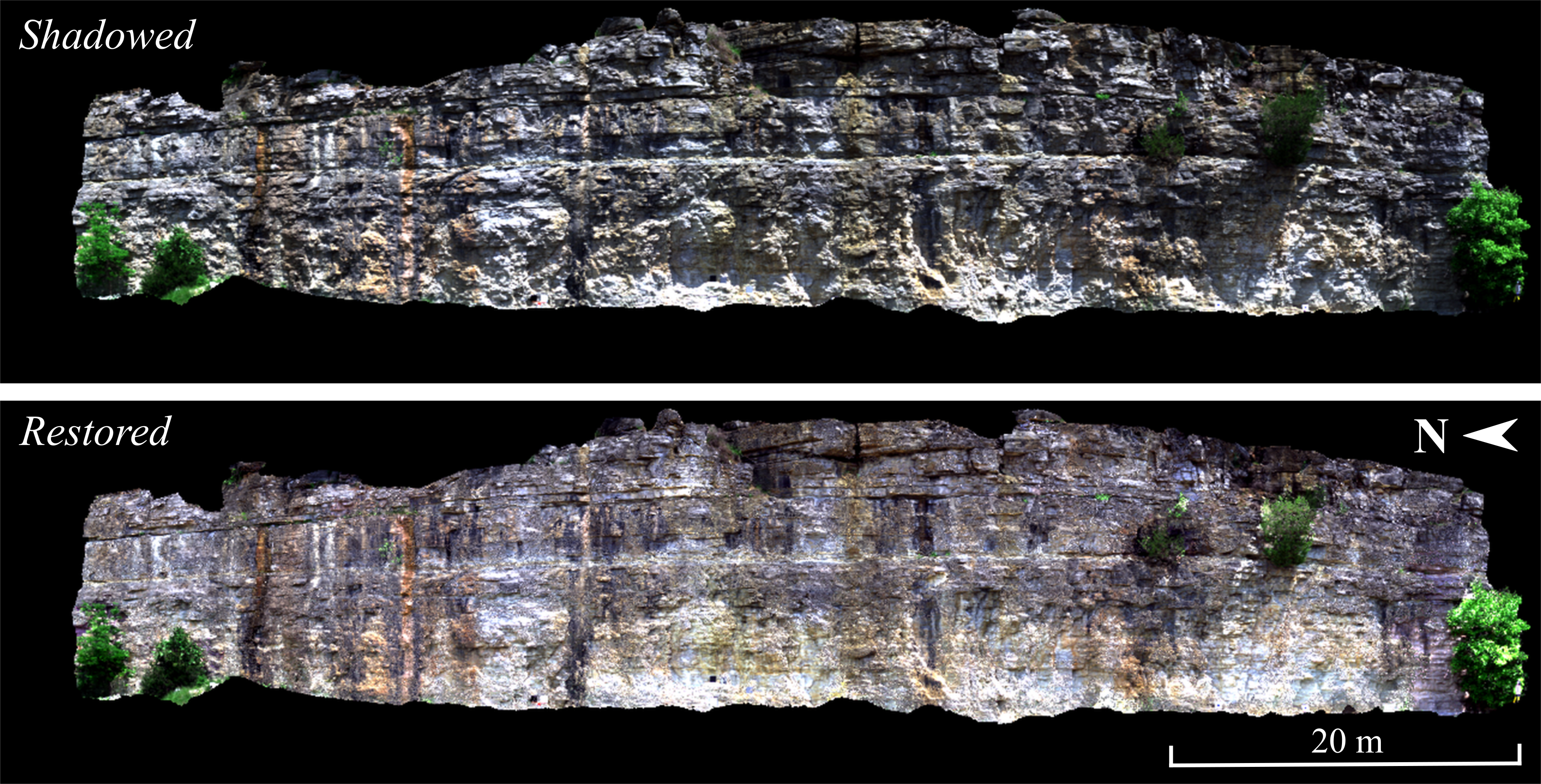
Using the solved IO and EO parameters, all HSI images were then co-registered into the pixel space of a single master image (the camera was moved between each setup), which was chosen to be the SWIR-sun image. Each master image pixel was projected into object space by solving for the intersection of the ray emanating from the pixel with the outcrop mesh generated from the TLS point data. These object space points were then projected into each slave image (the SWIR-shade and SWIR-partial images) and the spectra of the solved slave pixel locations used to generate images registered to the space of the master image. The slave pixel spectra were estimated using two-dimensional cubic interpolation in a band-by-band fashion to mitigate spatial artifacts and blurring that can occur when employing resampling methods that do not approximate the underlying continuous image, such as nearest neighbor or weighted average methods.
2.3.3. TLS Intensity Registration and Segmentation
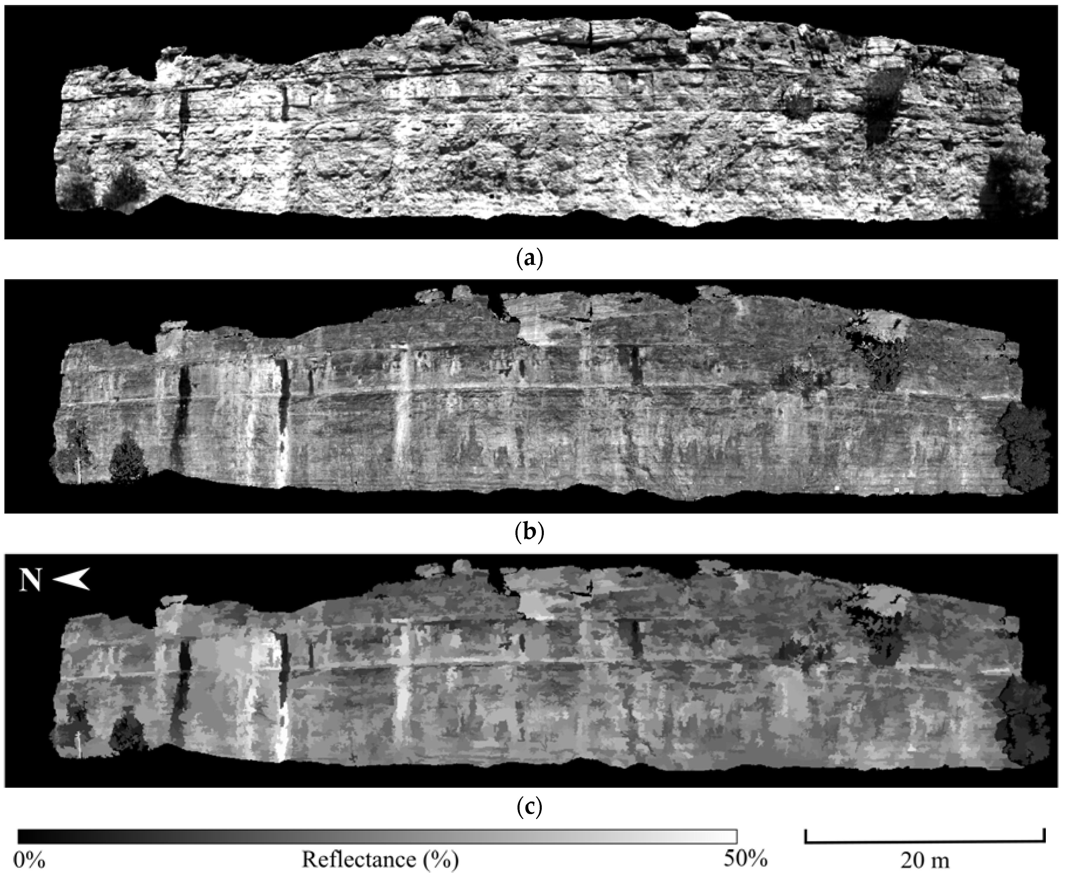
Eight-bit grayscale raster images of the radiometrically calibrated lidar intensity, i.e., active reflectance images, were created by projecting each TLS point through the camera model utilizing the master image IO and EO parameters. Since the point cloud was generated from multiple TLS instrument setups not collocated with the HSI camera, it was necessary to test the visibility of each point with respect to the camera prior to projecting the point through the camera model. This was accomplished by testing the ray from each TLS point to the camera for intersection with the mesh surface. Using only those points not occluded with respect to the camera, the mean active reflectance for each pixel was computed to generate a 1550 nm active reflectance image from the Riegl VZ-400 instrument. Figure 4 shows the 1550 nm active reflectance image compared to the closest wavelength band in the SWIR-sun HSI.
Several shadow restoration methods examined in this paper require the selection of regions of pixels containing similar material existing in both sun and shade areas. Given its resistance to solar shadowing, the active reflectance information is used to assist in the selection. Since both spatial and spectral proximity are relevant indicators of common material location, the active reflectance images were segmented into spatially connected regions of similar brightness values. This required a segmentation method able to tolerate stochastic variability in adjacent pixel brightness values while maintaining sensitivity to a systematic bias in brightness at larger spatial distances. The mean shift algorithm by [27] was chosen to meet these needs. The algorithm identifies the local modes of the underlying brightness density of an image (it treats image pixel brightness values as samples of a probability density function) and segments those pixels that are within each local mode’s “basin of attraction”. User input to the algorithm is limited to defining spatial (pixel) and spectral (brightness level) kernel bandwidths, which control the size of the segments, i.e., the amount of smoothing. A sample segmented 1550 nm active reflectance image created using spatial and spectral bandwidths of 20 pixels and 1 brightness unit (8-bit image brightness), respectively, is given in Figure 4c. The level of tolerance for stochastic variability in adjacent pixel brightness values was empirically determined by selecting those spatial and spectral bandwidths that produced the best shadow restoration results (see Section 3.2.1).
3. Methodology
3.1. HSI Pixel Shadow Determination
In order to restore HSI shadow spectra, the shadowed pixels must first be identified in the HSI. Shadow detection methods can be broadly divided into those based purely in image space and those which employ supporting structural information of the scene acquired from photogrammetry or lidar measurements. Image space shadow detection methods include histogram thresholding [28], region growing [29], color invariance techniques that separate chromaticity from intensity [30], matched filters using dark endmembers [15], unsupervised and supervised classification algorithms [31,32] and empirical HSI band indices [17]. The wide variety of methods reflects the difficulty in consistently achieving high accuracy results, particularly for low reflectance targets in sunlit regions and high reflectance targets in shadowed regions.
In contrast to image based methods, structural shadow detection is deterministic in nature with the quality of the results dependent on the density and accuracy of the structural model used for occlusion analysis and the quality of the registration between the structural and image information [32]. High accuracy georeferencing information and exact image exposure times are also required in order to correctly locate the sun position relative to the scene geometry. Although these requirements can be challenging for airborne imagery [17,31], they are achievable for TLS and terrestrially acquired HSI using standard data collection and processing methods. Ray tracing occlusion analysis [32], i.e., line-of-sight analysis, was therefore employed for shadow detection in this work.
Similar to the technique used to co-register the HSI imagery, each pixel center in the master image was projected onto the mesh model of the outcrop. The points on the mesh model were then projected in the direction of the sun and tested for intersection with the mesh model to determine the presence or absence of shadow in each pixel. In addition to this binary shadow determination, fractional shadow amounts within each pixel were also computed by applying the technique to four evenly spaced points within each pixel.
3.2. HSI Shadow Restoration
3.2.1. Indirect Shadow Restoration
One of the goals of this work is to examine the effectiveness of active reflectance information for identifying regions of similar material in sunlit and shadowed HSI pixels. This is examined through application of two existing shadow restoration techniques that utilize matching material regions: a mean scale correction and linear correlation correction. These techniques are termed “indirect” since the active reflectance information is not directly applied to the shadowed pixel spectra.
The mean scale correction is a basic technique that approximates the difference between sunlit and shadowed areas of a region of common material as a simple scale factor [33]. For a single HSI band with brightness values in a generic DN, the mean scale correction is given as
where and are mean values computed from sun and shade regions of similar material and is an original pixel brightness value in the shadowed area being corrected. Equation (1) is applied to images with brightness values in units of reflectance in this work. Pixels with fractional shadow assignments can also be incorporated, and both the binary and fractional shade detection products were tested with this method.
The linear correlation correction technique was chosen based on several studies that report its performance to be favorable in comparison to other standard statistical shadow restoration methods, such as histogram matching and gamma correction techniques [28,34,35]. The linear correlation correction, also referred to as the mean and variance transform, for restoring shadowed pixels within a single HSI band is given as
where is the standard deviation of a sun or shade region and all other terms are as defined for Equation (1). As with the mean scale correction, the linear correlation correction was applied to HSI converted to units of reflectance.
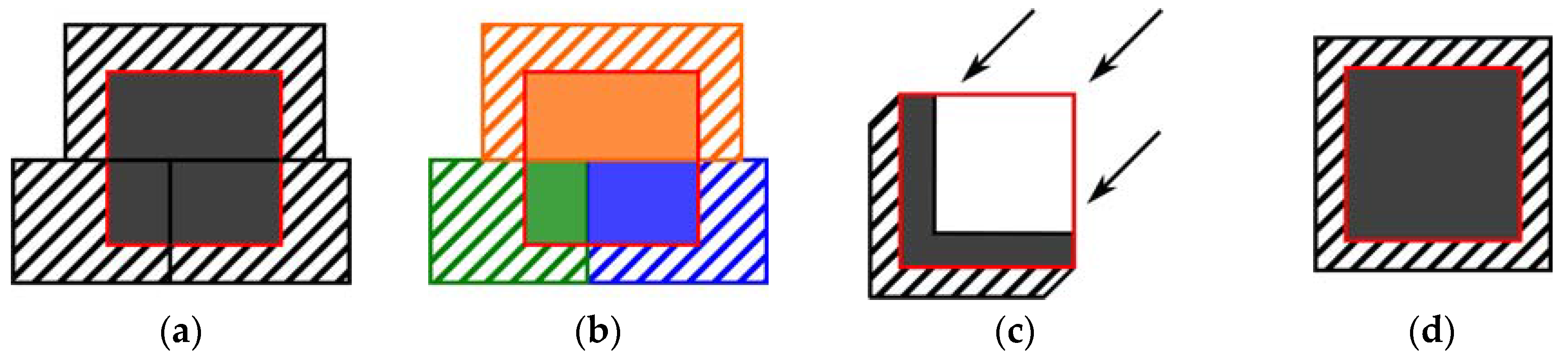
In order to evaluate the value of active reflectance information in the restoration methods, the required regions of similar material existing in the sun and shade are identified using either the segmented active reflectance information or spatial proximity only, which is the standard method. When using the segmented active reflectance information, the matching sun and shade regions are selected, and the shadow restoration algorithms applied, in the following two ways:
- Selection and restoration is applied to the union of all segments intersecting a shadow area, where the matching sun and shade regions are created from the combination of multiple contiguous active reflectance segments that intersect the shadow area of interest.
- Selection and restoration is applied segment by segment, where the matching sun and shade regions are restricted to exist within a common segment.
These selection methods are illustrated in Figure 5a,b. For comparison, the following two region selection methods based only on spatial proximity are used:
- Buffers of pixels along the far edge of the cast shadow, as in [36], one pushing into the sunlit area and the other into the shadowed area.
- The complete shadow area and a buffer of sunlit pixels around the entire boundary of the shadow area.
These methods are illustrated Figure 5c,d.
Prior to evaluating the relative performance of the different region selection and shadow restoration methods, the parameters used to select the regions of similar material in the sun and shade were optimized. For the region selection methods using the active reflectance information, the spatial and spectral ranges in the mean shift algorithm used to create the segmented images were varied; spatial pixel distances of 10, 20, 30 and 40 and spectral brightness distances (8-bit imagery) of 1, 2 and 3 were used. For the spatial proximity methods, the number of buffered pixels was varied with values of 2, 4, 8 and 16 used. The shadow restoration algorithms were then executed using the matching sun and shade regions generated from variable parameter sets defined above. In almost every case the parameters producing the greatest improvement in spectral shape, spectral scale or mean band correlation were not the same for a given restoration method. Therefore, the parameters producing the greatest improvement in spectral shape were selected since a small difference in spectrum shape can be more relevant to a material difference than a small difference in spectrum magnitude, e.g., when employing a spectral angle mapper (SAM) classifier.
3.2.2. Direct Shadow Restoration
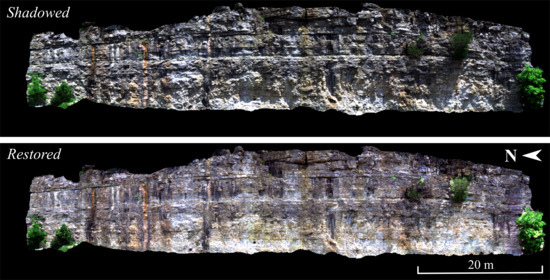
Rather than incorporating the active reflectance information into existing shadow restoration techniques, where it is used indirectly to assist in identifying similar material regions in the sun and shade, the active reflectance can be used to directly adjust the passive pixel spectra. The direct adjustment is a simple scale factor, derived from the ratio of the active (TLS) to passive (HSI) reflectance measures at the active reflectance wavelength (the TLS laser wavelength), which is then applied to the entire passive spectrum of the subject pixel. This is illustrated in Figure 6, where sample original (shadowed) and directly scaled pixel spectra from a single pixel location are shown and compared to the spectrum of a sunlit pixel of similar material. Note that the direct adjustment is applied to all pixels in the HSI, both those in the shade and in the sun.
The drawback to this method is the coarse assumption that the spectrum of irradiance incident on shadowed surfaces is simply an attenuated version of that on sunlit surfaces. The error in this assumption is readily apparent in the scaled spectrum shown in Figure 6. However, if multiple active reflectance wavelengths falling within the spectral range of the HSI were available, i.e., multispectral lidar, an interpolated scale factor could be applied across the spectrum to mitigate the error. This possibility was simulated through the application of three commercially viable lidar wavelengths (1064, 1550, and 2050 nm) to the shadowed spectra as well as uniformly spaced sets of wavelengths that are only possible with white laser sources (e.g., [37,38]).
3.2.3. Restoration Metrics
Metrics defining spectral shape, spectral scale, and band correlation with a truth image are used to quantify shadow restoration effectiveness. Spectral shape is defined as
where and are the pixel spectrum vectors being compared, and as approaches the metric approaches unity. Note that the spectral shape metric is the cosine of the spectral angle, which is the basis of the SAM classifier that is often applied to imagery with variable illumination intensity.
Spectral scale quantifies the mean scalar difference between two pixel spectrums and is defined as
where the division of spectrum vector by is performed wavelength-by-wavelength. As with spectral shape, the metric approaches unity as approaches .
In Equations (3) and (4), is a sunlit pixel in the partial sun image and is a shadowed pixel of similar material existing in the same image. After restoration of , the movement of both the spectral shape and scale towards unity indicates improvement in agreement with . Although the effectiveness of pixel spectrum restoration could be done by comparing shadowed pixels from a partial shade image to sunlit pixels at the same location in the corresponding registered maximum sun image (e.g., SWIR-partial versus SWIR-sun), we chose to compute these metrics within, rather than between, images. This eliminates ambiguity associated with the distinct radiometric calibration applied to each image and any temporal differences in localized sky and topographic scattering characteristics existing between images. The locations of sun/shade pixel pairs containing similar materials were identified in the maximum sun image as those pairs with a spectral shape metric greater than 0.9995 and spectral scale metric between 0.95 and 1.05. Potential pixel pair locations were constrained such that one pixel was located in the shade and one in the sun in the partial shade image being restored. Over 1000 pixel pairs were identified in the SWIR-partial image.
The final metric, band correlation, quantifies the similarity between two HSI bands and is defined as
where is a vector of all pixel brightness values in a single band of the full shade image and is the corresponding vector of band values from an original or restored partial shade image. The full shade images are used for comparison given their very uniform appearance due to the absence of solar shadowing. The application of the band correlation metric to partial shade bands before and after shadow restoration quantifies the “eye-test” naturally applied to a corrected band, i.e., random speckle or poorly corrected shadow regions that are easily identified visually will produce lower correlation values. To ease interpretation, a mean band correlation computed from the collection of all image band correlation values is used.
4. Results and Discussion
4.1. Shadow Determination
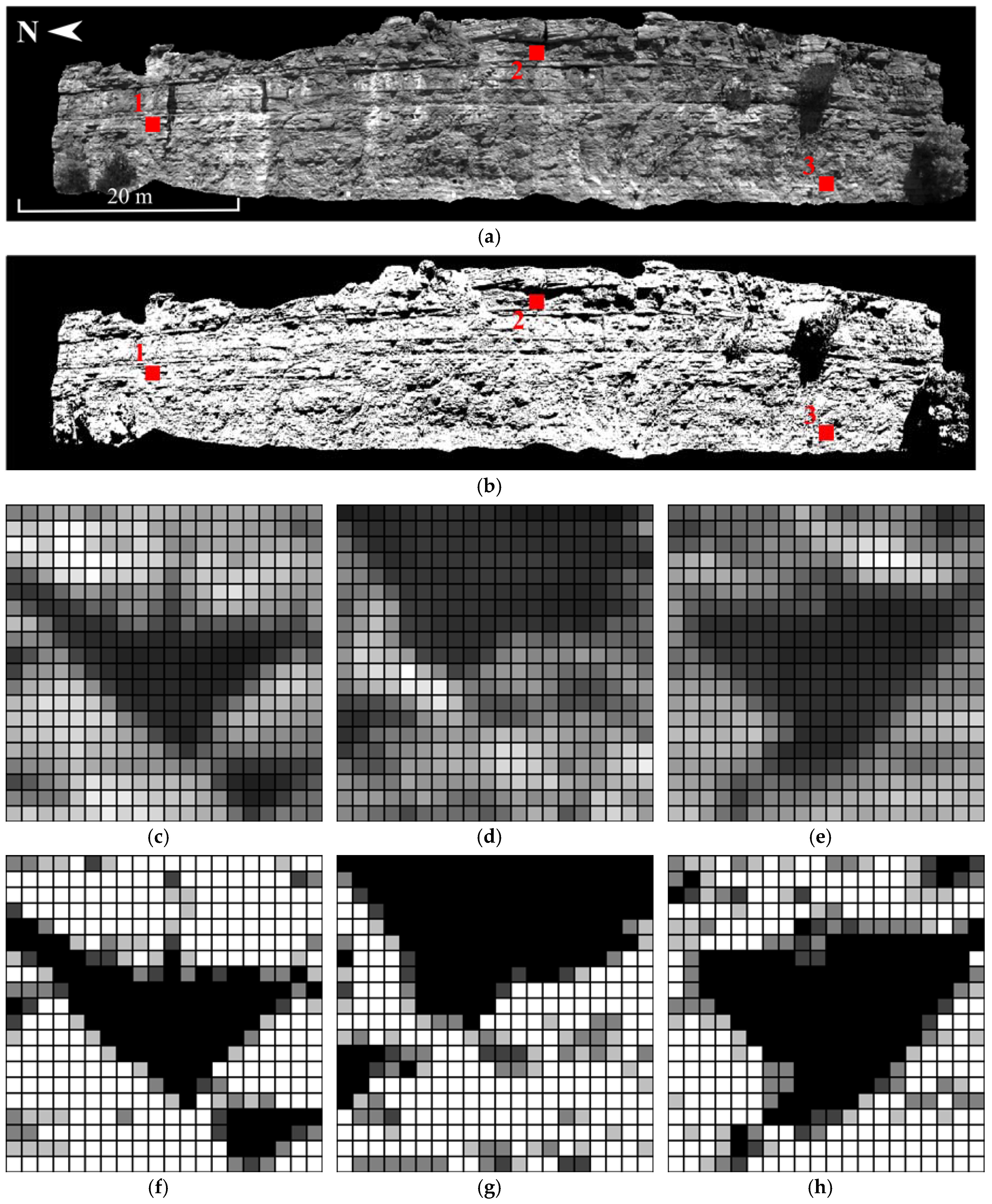
Shadow determination accuracy is difficult to quantify since it requires visual identification of exact shadow edges in the imagery, which is complicated by the influence of both shadow and material differences on pixel brightness values. However, qualitative visual comparison of multiple well-defined shadow features across the surface of the outcrop suggests a pixel-level accuracy (see Figure 7). This qualitative assessment is indirectly validated by a reduction in over- and under-corrected pixel brightness values, as evidenced by improvements in the band correlation metric, produced by the scalar shadow restoration algorithm when using fractional, rather than binary, shadow detection results. This observation is expanded further in the following discussion of the shadow restoration results. It is noted that the shadow detection method is not robust for vegetation, whose complex structure is not adequately modeled by the mesh surface model.
4.2. Shadow Restoration
4.2.1. Indirect Restoration
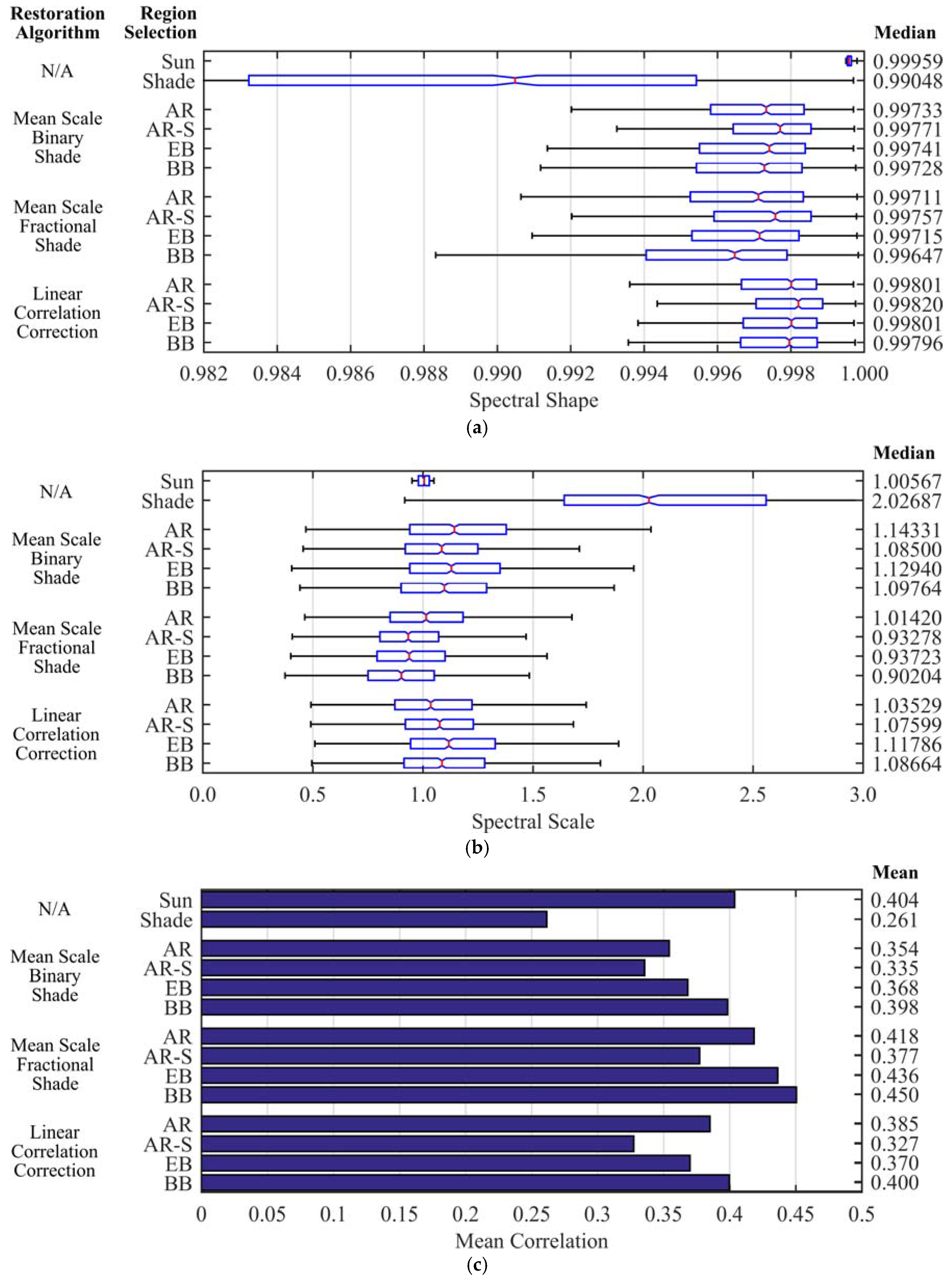
Results for the mean scale restoration method, for both the binary and fractional (1/4 fraction) shadow products, and the linear correlation correction method are given in Figure 8 for the SWIR-partial HSI. Each of the four matching region selection techniques were applied to each shadow restoration method. Boxplots illustrating the median and interquartile (IQR) ranges of the spectral shape and scale metrics of the matched pixel pairs were chosen for ease of comparison of the skewed distributions, while mean band correlation improvement is compared with a bar graph. The metrics computed from the maximum sun and unrestored partial shade image are shown at the top of each graph for reference. In general, all combinations of the restoration methods and region selection techniques improved the shadowed pixel spectra. The average improvement in median and interquartile range (IQR), as defined by the percentage by which the restored median and IQR values move toward the reference (sun) median and IQR values, is 77% and 80% for the spectral shape metric, and 92% and 66% for the spectral scale metric.
Recalling that the region selection parameters were optimized for the spectral shape metric, the use of active reflectance for region selection has a small positive influence on spectral shape restoration for all three restoration methods, but only when applying the active reflectance information in a segment by segment manner. However, using the active reflectance in a segment by segment fashion produces spatial discontinuities in brightness that follow the segment boundaries when applying the mean scale method and mottling when applying the linear correlation correction method. The linear correlation correction method performs the best among the three restoration methods, which is in agreement with the results of prior research by others [28,34,35].
The spectral scale results do not exhibit a trend between region selection techniques. With respect to restoration methods, it is observed that slightly lower values are generated by the fractional shade mean scale restoration method. This systematic difference is due to the use of fractional, rather than binary (which are used in the other restoration methods), shade values, which alters both the computation and application of the mean scale factor.
For mean band correlation, the use of active reflectance information for region selection has an overall negative influence on the restoration methods, with the exception of the linear correlation correction method. In particular the application of the restoration methods in a segment by segment fashion based on active reflectance information is always the lowest. This is due to the previously mentioned jigsaw and mottling artifacts. Note that the mean scale restoration method using fractional, as opposed to binary, shade values produces higher band correlation values for all region selection techniques. This is a result of slightly “smoother” band images that are produced in comparison to the methods using the binary shadow computation. The smoothness reflects an improvement in the amount of correction applied to each pixel, and is an indirect validation of the shadow detection accuracy at the sub-pixel, i.e., fractional, level.
In summary, the influence of active reflectance information on determining regions of similar materials is marginal in comparison to region matching methods based purely on spatial information. Improvements in spectral shape restoration when using regions defined by active reflectance is limited to when they are applied in a segment by segment fashion, but this improvement comes at the cost of reduced band correlation due to spatial artifacts.
4.2.2. Single Wavelength Direct Restoration
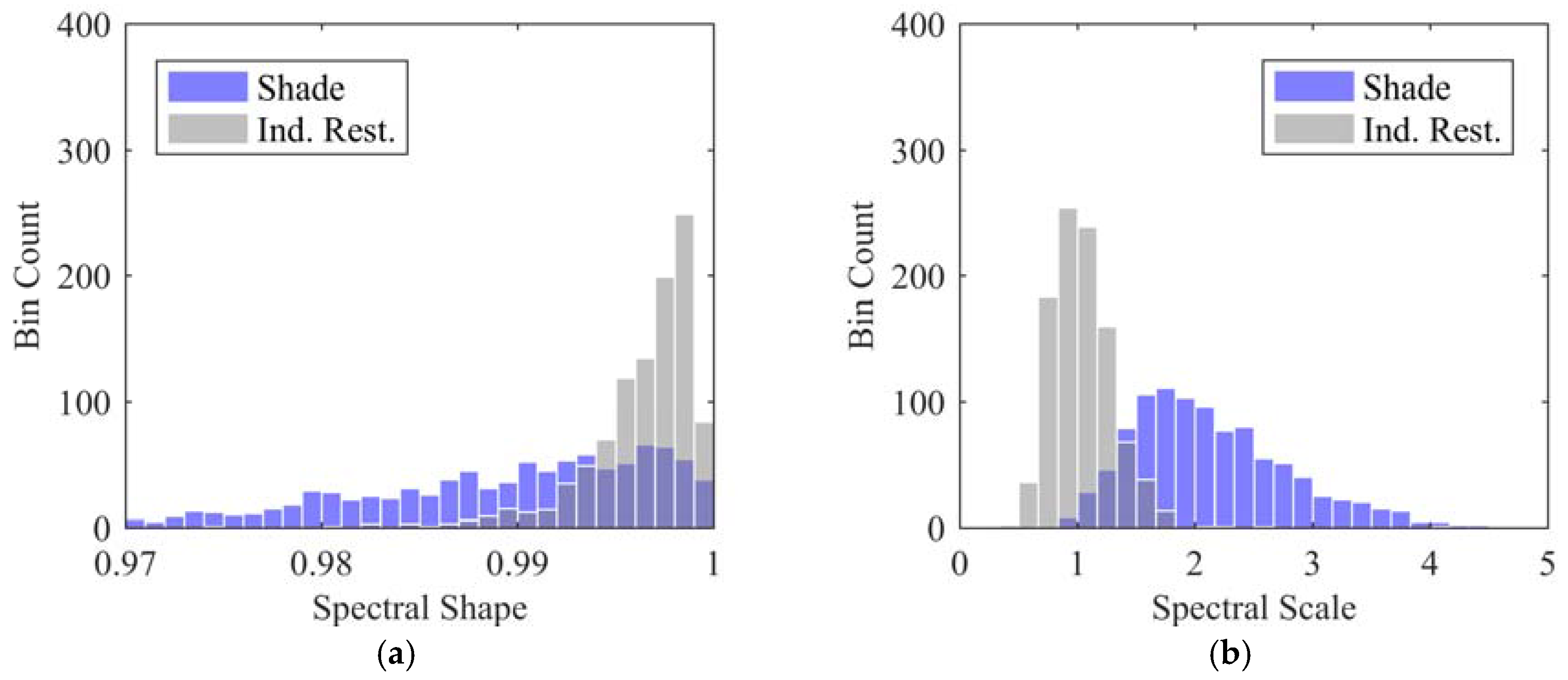
When applying a single scale factor to a pixel spectrum, there is no change to the shape of the spectrum and thus no improvement in the spectral shape metric. However, there is distinct improvement in spectrum scale, beyond that achieved by the indirect restoration methods previously examined. These two observations can be seen by comparing Figure 9a,c and Figure 9b,d, respectively. Figure 9 contains histograms of the spectral shape and spectral scale metrics before and after application of the indirect and direct restoration algorithms to the shade spectrum of each of the ~1000 matched material sun and shade pixel pairs. The IQR of the spectral scale histogram generated from the directly scaled HSI is reduced by 39% and over its indirectly restored counterpart. Band correlation is shown in Figure 10 and is improved from approximately 0.4 to 0.6, a 45% improvement, resulting from the removal of uncompensated topography-induced solar irradiance differences and the error associated with imperfect pixel shadow determination.
The computed scale factors are most applicable very near the scaling wavelength, with large differences between the scaled and sunlit spectra occurring away from the scaling wavelength, e.g., see Figure 6. This motivates the application of one of the indirect shadow restoration methods on top of a directly scaled HSI, thereby improving both spectrum magnitude and shape. Histograms of the improvements for all matched sun/shade pixel pairs are shown in Figure 9e,f and an example spectrum is shown in Figure 6. However, the improvement in spectral shape is slightly less than achieved with purely indirect restoration methods, and the improvement in spectral scale is slightly less than with the purely direct scale application. Finally, the application of dual correction techniques also improves the band correlation of the directly scaled HSI by approximately 6% in the 1000–1300 nm wavelength region (Figure 10).
4.2.3. Multiple Wavelength Direct Restoration Simulation
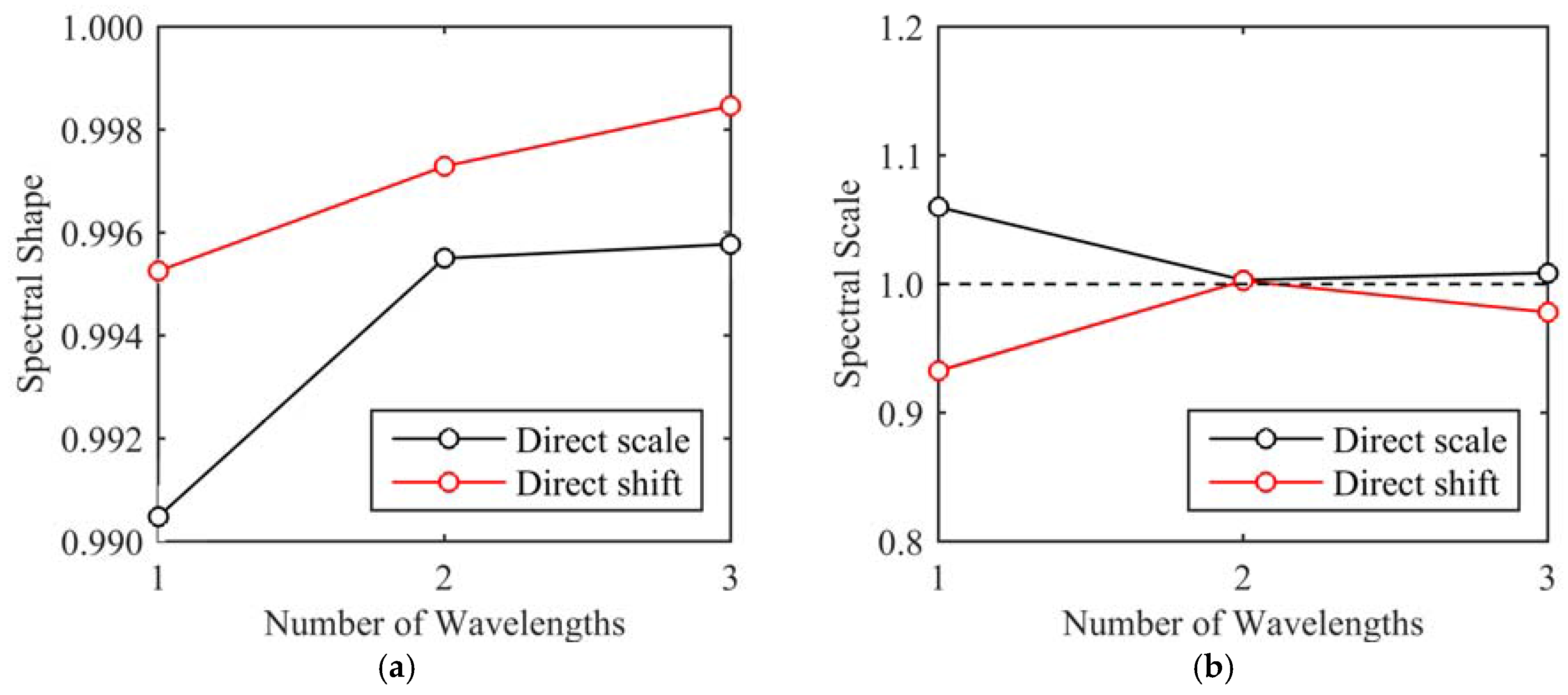
Although the application of a direct scale factor followed by an indirect restoration method combines the positive aspects of both techniques, the indirect restoration methods are computationally heavy, requiring detection and restoration of each distinct shadow area. If multiple active reflectance wavelengths were available within the spectrum of a single HSI, an interpolated direct scale factor could be applied between the active reflectance wavelengths, thus easing computational loads while potentially restoring spectrum shape. A multiple wavelength direct adjustment was therefore simulated using commercially available or viable lidar wavelengths that fall within the spectrum of the SWIR HSI (1064, 1550, and 2050 nm). The shade spectrum for each matched shade/sun pixel pair used in the prior indirect restoration analysis was then iteratively scaled using successively greater numbers of scaling wavelengths. The simulated scale factors were computed from the ratio of the sun to shade spectrum values at each selected laser wavelength. For spectrum locations between scaling wavelengths, the scale factors were linearly interpolated. The resulting improvements in the median values of the spectral shape and spectral scale metrics as a function of the number of scaling wavelengths are plotted in Figure 11.
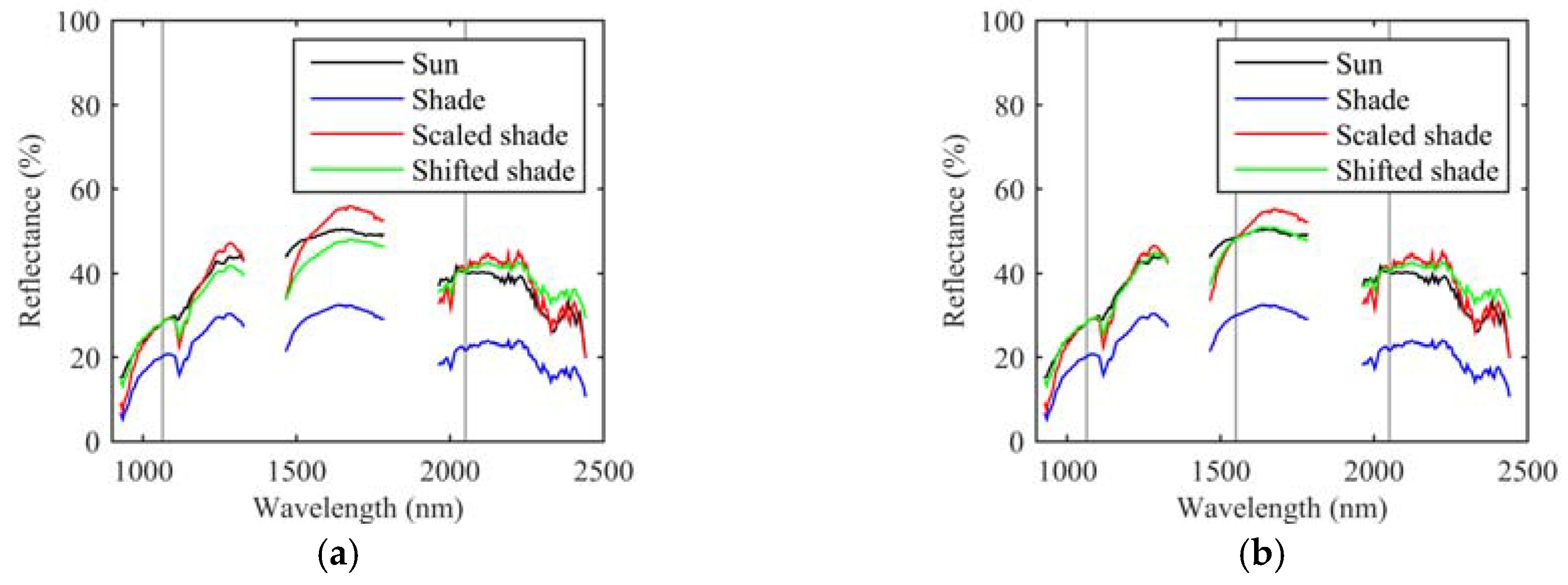
Figure 12 shows a representative scaled shade spectrum from a matched sun/shade pixel pair (the same spectra are shown in Figure 6) for two and three wavelength scale locations. Note that, even with multiple wavelength scaling locations, the scaled shade spectra still differ from the sun spectrum shape. If we discard the physical premise that the influence of shade on material spectra is roughly scalar and instead apply an interpolated spectrum shift (i.e., a translation) computed at the selected wavelength locations, the agreement in shape appears to be improved. The improvement is quantified by applying the shift adjustment to the entire set of matched sun/shade pixel pairs (see Figure 11). Note that the simulation does not consider the errors that would normally exist if the scale or shift values were derived from actual active (TLS) reflectance information.
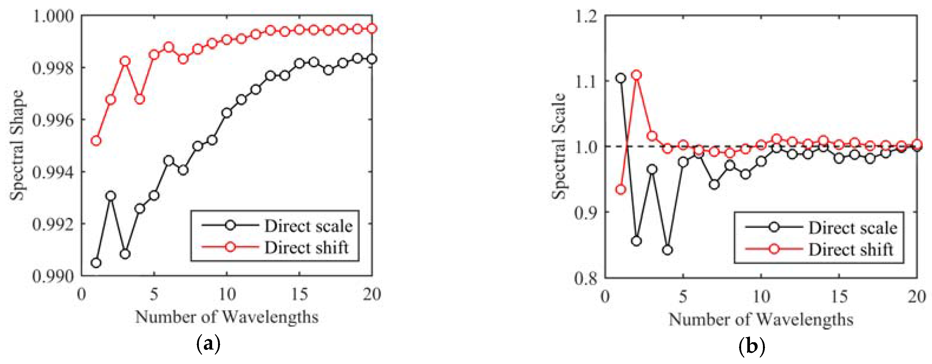
Figure 13 illustrates the influence of additional scale or shift wavelength locations beyond those currently commercially available. The wavelength locations were uniformly distributed in the simulation. Although not practically realizable, the results indicate a ceiling on spectrum improvement as the number of wavelength locations is increased. The shift adjustment stabilizes more quickly than the scale adjustment, with the majority of improvement achieved with 8–10 uniformly spaced wavelengths. These results may be applicable to hyperspectral lidar systems, which currently only record backscattered laser intensity at a relatively small number of discrete wavelengths (e.g., [37,39,40]).
5. Conclusions
The inclusion of radiometrically calibrated TLS intensity in several statistics-based image shadow restoration algorithms for the purpose of identifying regions of similar material was demonstrated for HSI collected from a terrestrial modality. Although only a marginal improvement in shadow restoration compared to purely spatial region matching methods was achieved, including TLS intensity information does not add a significant cost in terms of complexity or processing time. It is possible that scenes with greater variation in material spectra at the TLS laser wavelength than the geologic outcrop used in this study would experience a greater benefit from the inclusion of TLS intensity for material matching.
An alternative method for utilizing radiometrically calibrated TLS intensity in HSI shadow restoration is to directly scale every pixel spectrum, regardless of whether a pixel is sunlit or shadowed, by the ratio of the TLS and HSI reflectance values at their common wavelength. This method greatly simplifies the shadow restoration process since identification of shadowed pixels and matching material regions is not required. However, it relies on the improper assumption that surface irradiance in shadows can be estimated as a scaled version of surface irradiance in sunlit areas and therefore does not improve shadowed pixel spectrum shape. This deficiency can be mitigated by combining the scaled HSI with region matching restoration algorithms, thereby improving both spectrum shape and scale, but at the cost of reintroducing shadow identification and region matching complexity to the restoration process. Although only able to be simulated, the introduction of multiple lidar laser wavelengths enables an interpolated scale or shift to be applied to HSI pixel spectrum, which was shown to improve both spectrum magnitude and shape. This method does not require shadow identification or region matching and may be applicable to hyperspectral lidar sensors currently under development, e.g., those being developed at the Finnish Geodetic Institute [37,40], that only record backscattered laser energy at a relatively small number of discrete wavelengths.
The analysis in this paper focused on spectral shape, spectral scale, and band correlation metrics to quantify shadow restoration effectiveness in terrestrial HSI. A primary application of HSI, regardless of the collection modality, is material identification, i.e., image classification. Future work will therefore examine the effectiveness of the proposed methods on improving material classification in shadowed pixels, as well as validation of the simulated multiple wavelength direct restoration technique.
Acknowledgments
This work was supported in part by the U.S. Army Engineer Research and Development Center Cold Regions Research and Engineering Laboratory Remote Sensing/GIS Center of Expertise.
Author Contributions
Preston Hartzell performed the analysis and wrote the manuscript. Craig Glennie guided the research and contributed to improving the manuscript. Shuhab Khan organized the field collection of data.
Conflicts of Interest
The funding sponsors had no role in the design of the study; in the collection, analyses, or interpretation of data; in the writing of the manuscript, and in the decision to publish the results.
References
- Schaepman, M.E.; Ustin, S.L.; Plaza, A.J.; Painter, T.H.; Verrelst, J.; Liang, S. Earth system science related imaging spectroscopy—An assessment. Remote Sens. Environ. 2009, 113, S123–S137. [Google Scholar] [CrossRef]
- Goetz, A.F.H. Three decades of hyperspectral remote sensing of the Earth: A personal view. Remote Sens. Environ. 2009, 113, S5–S16. [Google Scholar] [CrossRef]
- Buckley, S.J.; Kurz, T.H.; Howell, J.A.; Schneider, D. Terrestrial lidar and hyperspectral data fusion products for geological outcrop analysis. Comput. Geosci. 2013, 54, 249–258. [Google Scholar] [CrossRef]
- Kurz, T.H.; Buckley, S.J.; Howell, J.A. Close-range hyperspectral imaging for geological field studies: Workflow and methods. Int. J. Remote. Sens. 2013, 34, 1798–1822. [Google Scholar] [CrossRef]
- Kurz, T.H.; Buckley, S.J.; Howell, J.A.; Schneider, D. Integration of panoramic hyperspectral imaging with terrestrial lidar data. Photogramm. Rec. 2011, 26, 212–228. [Google Scholar] [CrossRef]
- Kurz, T.H.; Dewit, J.; Buckley, S.J.; Thurmond, J.B.; Hunt, D.W.; Swennen, R. Hyperspectral image analysis of different carbonate lithologies (limestone, karst and hydrothermal dolomites): The Pozalagua Quarry case study (Cantabria, North-west Spain). Sedimentology. 2012, 59, 623–645. [Google Scholar] [CrossRef]
- Murphy, R.J.; Schneider, S.; Taylor, Z.; Nieto, J. Mapping clay minerals in an open-pit mine using hyperspectral imagery and automated feature extraction. In Proceedings of the Vertical Geology Conference, Lausanne, Switzerland, 6–7 February 2014. [Google Scholar]
- Murphy, R.J.; Monteiro, S.T. Mapping the distribution of ferric iron minerals on a vertical mine face using derivative analysis of hyperspectral imagery (430–970nm). ISPRS J. Photogramm. Remote Sens. 2013, 75, 29–39. [Google Scholar] [CrossRef]
- Murphy, R.J.; Monteiro, S.T.; Schneider, S. Evaluating Classification Techniques for Mapping Vertical Geology Using Field-Based Hyperspectral Sensors. IEEE Trans. Geoscience Remote Sens. 2012, 50, 3066–3080. [Google Scholar] [CrossRef]
- Clark, R.N. Chapter 1: Spectroscopy of Rocks and Minerals, and Principles of Spectroscopy. In Manual of Remote Sensing, Remote Sensing for the Earth Sciences; Rencz, A.N., Ed.; John Wiley & Sons: New York, NY, USA, 1999; Volume 3, pp. 3–58. [Google Scholar]
- Van der Meer, F.D.; van der Werff, H.M.A.; van Ruitenbeek, F.J.A.; Hecker, C.A.; Bakker, W.H.; Noomen, M.F.; van der Meijde, M.; Carranza, E.J.M.; de Smeth, J.B.; Woldai, T. Multi- and hyperspectral geologic remote sensing: A review. Int. J. Appl. Earth Obs. Geoinform. 2012, 14, 112–128. [Google Scholar] [CrossRef]
- Buckley, S.J.; Enge, H.D.; Carlsson, C.; Howell, J.A. Terrestrial laser scanning for use in virtual outcrop geology. Photogramm. Rec. 2010, 25, 225–239. [Google Scholar] [CrossRef]
- Alexander, J. A discussion on the use of analogues for reservoir geology. Geol. Soc. Lond. Spec. Publ. 1992, 69, 175–194. [Google Scholar] [CrossRef]
- Ientilucci, E.J. SHARE 2012: Analysis of illumination differences on targets in hyperspectral imagery. Proc. SPIE 2013. [Google Scholar] [CrossRef]
- Adler-Golden, S.M.; Matthew, M.W.; Anderson, G.P.; Felde, G.W.; Gardner, J.A. An Algorithm for De-Shadowing Spectral Imagery. In Proceedings of the 11th JPL Airborne Earth Science Workshop, Pasadena, CA, USA, 5–8 March 2002. [Google Scholar]
- Friman, O.; Tolt, G.; Ahlberg, J. Illumination and shadow compensation of hyperspectral images using a digital surface model and non-linear least squares estimation. In Proceedings of the SPIE 8180, Image and Signal Processing for Remote Sensing XVII, Prague, Czech Republic, 19 September 2011. [Google Scholar]
- Schläpfer, D.; Richter, R.; Damm, A. Correction of Shadowing in Imaging Spectroscopy Data by Quantification of the Proportion of Diffuse Illumination. In Proceedings of the 8th SIG-IS EARSeL Imaging Spectroscopy Workshop, Nantes, France, 8–10 April 2013. [Google Scholar]
- Anderson, G.P.; Felde, G.W.; Hoke, M.L.; Ratkowski, A.J.; Cooley, T.; Chetwynd, J.H.; Gardner, J.A.; Adler-Golden, S.M.; Matthew, M.W.; Berk, A.; et al. MODTRAN4-based atmospheric correction algorithm: FLAASH (fast line-of-sight atmospheric analysis of spectral hypercubes). In Proceedings of the SPIE 4725, Algorithms and Technologies for Multispectral, Hyperspectral, and Ultraspectral Imagery VIII, Orlando, FL, USA, 1 April 2002. [Google Scholar]
- Richter, R.; Schläpfer, D. Geo-atmospheric processing of airborne imaging spectrometry data. Part 2: Atmospheric/topographic correction. Int. J. Remote Sens. 2002, 23, 2631–2649. [Google Scholar] [CrossRef]
- Hartzell, P.J.; Glennie, C.L.; Finnegan, D.C. Empirical Waveform Decomposition and Radiometric Calibration of a Terrestrial Full-Waveform Laser Scanner. IEEE Trans. Geosci. Remote Sens. 2015, 53, 162–172. [Google Scholar] [CrossRef]
- Kazhdan, M.; Hoppe, H. Screened poisson surface reconstruction. ACM Trans. Graph. 2013, 32, 1–13. [Google Scholar] [CrossRef]
- CloudCompare (Version: 2.6.1). Available online: http://www.cloudcompare.org/ (accessed on 15 May 2015).
- Han, T.; Goodenough, D.G.; Dyk, A.; Love, J. Detection and correction of abnormal pixels in Hyperion images. In Proceedings of the IEEE International Geoscience and Remote Sensing Symposium, Toronto, ON, Canada, 23–28 July 2002. [Google Scholar]
- Schneider, D.; Maas, H.G. A geometric model for linear-array-based terrestrial panoramic cameras. Photogramm. Rec. 2006, 21, 198–210. [Google Scholar] [CrossRef]
- Scheibe, K.; Huang, F.; Klette, R. Calibration of Rotating Sensors. Proceedings of Computer Analysis of Images and Pattern, Münster, Germany, 2–4 September 2009. [Google Scholar]
- Hartzell, P.J. Active and Passive Sensor Fusion for Terrestrial Hyperspectral Image Shadow Detection and Restoration. Ph.D. Dissertation, University of Houston, Houston, TX, USA, May 2016. [Google Scholar]
- Comaniciu, D.; Meer, P. Mean shift: A robust approach toward feature space analysis. IEEE Trans. Pattern Anal. Mach. Intell. 2002, 24, 603–619. [Google Scholar] [CrossRef]
- Dare, P.M. Shadow Analysis in High-Resolution Satellite Imagery of Urban Areas. Photogramm. Eng. Remote Sens. 2005, 71, 169–177. [Google Scholar] [CrossRef]
- Xia, H.; Chen, X.; Guo, P. A shadow detection method for remote sensing images using Affinity Propagation algorithm. In Proceedings of the IEEE International Conference on Systems, Man and Cybernetics, San Antonio, TX, USA, 5–8 October 2009. [Google Scholar]
- Tsai, V.J.D. A comparative study on shadow compensation of color aerial images in invariant color models. IEEE Trans. Geosci. Remote Sens. 2006, 44, 1661–1671. [Google Scholar] [CrossRef]
- Tolt, G.; Shimoni, M.; Ahlberg, J. A shadow detection method for remote sensing images using VHR hyperspectral and LIDAR data. In Proceedings of the IEEE International Geoscience and Remote Sensing Symposium, Vancouver, BC, Canada, 23–28 July 2011. [Google Scholar]
- Adeline, K.R.M.; Chen, M.; Briottet, X.; Pang, S.K.; Paparoditis, N. Shadow detection in very high spatial resolution aerial images: A comparative study. ISPRS J. Photogramm. Remote Sens. 2013, 80, 21–38. [Google Scholar] [CrossRef]
- Fredembach, C.; Finlayson, G. Simple Shadow Removal. In Proceedings of the 18th International Conference on Pattern Recognition, Hong Kong, China, 20–24 August 2006. [Google Scholar]
- Sarabandi, P.; Yamazaki, F.; Matsuoka, M.; Kiremidjian, A. Shadow detection and radiometric restoration in satellite high resolution images. In Proceedings of the IEEE International Geoscience and Remote Sensing Symposium, Anchorage, AK, USA, 20–24 September 2004. [Google Scholar]
- Zhou, W.; Huang, G.; Troy, A.; Cadenasso, M.L. Object-based land cover classification of shaded areas in high spatial resolution imagery of urban areas: A comparison study. Remote Sens. Environ. 2009, 113, 1769–1777. [Google Scholar] [CrossRef]
- Li, Y.; Gong, P.; Sasagawa, T. Integrated shadow removal based on photogrammetry and image analysis. Int. J. Remote Sens. 2005, 26, 3911–3929. [Google Scholar] [CrossRef]
- Hakala, T.; Suomalainen, J.; Kaasalainen, S.; Chen, Y. Full waveform hyperspectral LiDAR for terrestrial laser scanning. Opt. Express 2012, 20, 7119. [Google Scholar] [CrossRef] [PubMed]
- Junttila, S.; Kaasalainen, S.; Vastaranta, M.; Hakala, T.; Nevalainen, O.; Holopainen, M. Investigating bi-temporal hyperspectral lidar measurements from declined trees-Experiences from laboratory test. Remote Sens. 2015, 7, 13863–13877. [Google Scholar] [CrossRef]
- Powers, M.A.; Davis, C.C. Spectral LADAR: Active range-resolved three-dimensional imaging spectroscopy. Appl. Opt. 2012, 51, 1468–1478. [Google Scholar] [CrossRef] [PubMed]
- Vauhkonen, J.; Hakala, T.; Suomalainen, J.; Kaasalainen, S.; Nevalainen, O.; Vastaranta, M.; Holopainen, M.; Hyyppa, J. Classification of Spruce and Pine Trees Using Active Hyperspectral LiDAR. IEEE Geosci. Remote Sens. Lett. 2013, 10, 1138–1141. [Google Scholar] [CrossRef]
Figure 1.
Quarry wall in: (a) full shade; (b) partial sun; and (c) maximum sun conditions.

Figure 2.
(a) Short wave infrared (SIWR, foreground) and visible to near infrared (VNIR, background) hyperspectral cameras attached to a tripod-mounted rotation stage. The cameras can be rotated vertically as well as horizontally. (b) Illustration of the disk swept by the rotating SWIR camera projection center (PC) as it revolves around the rotation center (RC). The parameters and define the location of the PC relative to the RC.

Figure 3.
Least squares resection adjustment residuals.
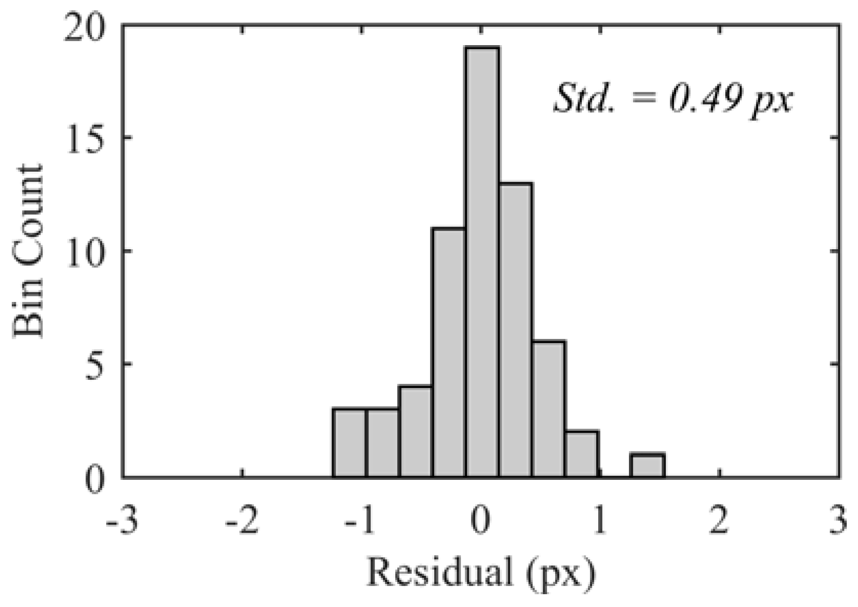
Figure 4.
(a) 1549 nm passive; and (b) 1550 nm active reflectance images. A mean shift segmented 1550 nm active reflectance image is shown in (c).
Figure 4.
(a) 1549 nm passive; and (b) 1550 nm active reflectance images. A mean shift segmented 1550 nm active reflectance image is shown in (c).

Figure 5.
Region selection methods: (a) union of active reflectance segments; (b) active reflectance segments, segment by segment; (c) cast shadow far edge buffer (arrows indicate solar ray direction); and (d) shadow boundary buffer. The red square indicates the shadow area, the rectangles in (a) and (b) represent active reflectance segments, solid fill indicates the selected portion of the shadow region, and diagonal hatching indicates the selected sun region.

Figure 6.
Example of a directly restored shade pixel spectrum through application of a scale factor (Dir. Rest.). The result of an indirect restoration after the direct scale restoration is also shown (Dir. +Ind. Rest.). The original shade and matched sun pixel spectra are shown for reference.
Figure 6.
Example of a directly restored shade pixel spectrum through application of a scale factor (Dir. Rest.). The result of an indirect restoration after the direct scale restoration is also shown (Dir. +Ind. Rest.). The original shade and matched sun pixel spectra are shown for reference.
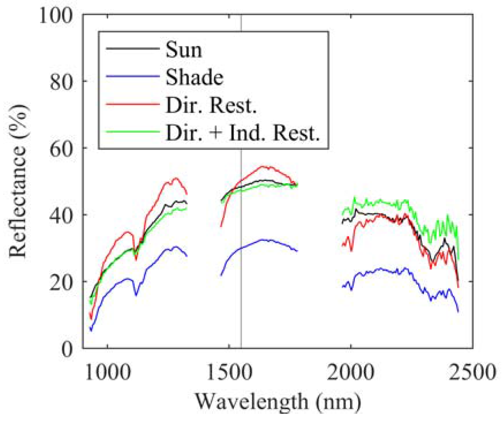
Figure 7.
(a) SWIR-sun 1549 nm band; (b) fractional (1/4 increment) pixel shadow determination; (c–e) detail locations 1–3 as indicated in (a,b); and (f–h) matching shadow determination for detail locations 1–3, where the gray value corresponds to the shadow fraction (white = full sun and black = full shade). Pixel dimensions in (c–h) are approximately 6 cm.

Figure 8.
Comparison of region selection methods on the mean scale and linear correlation correction shadow restoration metrics of: (a) spectral shape; (b) spectral scale; and (c) mean band correlation. Note the mean scale correction method is applied using a single shadow determination per pixel (binary) and using a 1/4 fraction shadow determination per pixel (fractional). The region selection methods using lidar intensity segments are: AR = Active Reflectance and AR-S = Active Reflectance-Segment by segment. The spatial region selection methods are: EB = Edge Buffer, BB = Boundary Buffer.

Figure 9.
Histograms illustrating the improvement (movement to toward a value of 1) in shadowed pixel spectral shape and scale metrics for the ~1000 matched material sun and shade pixel pairs when applying: (a,b) the indirect mean scale shadow restoration method; (c,d) direct scale restoration of the shadowed pixel spectra,; and (e,f) a direct scale to the pixel spectra followed by the indirect restoration method.

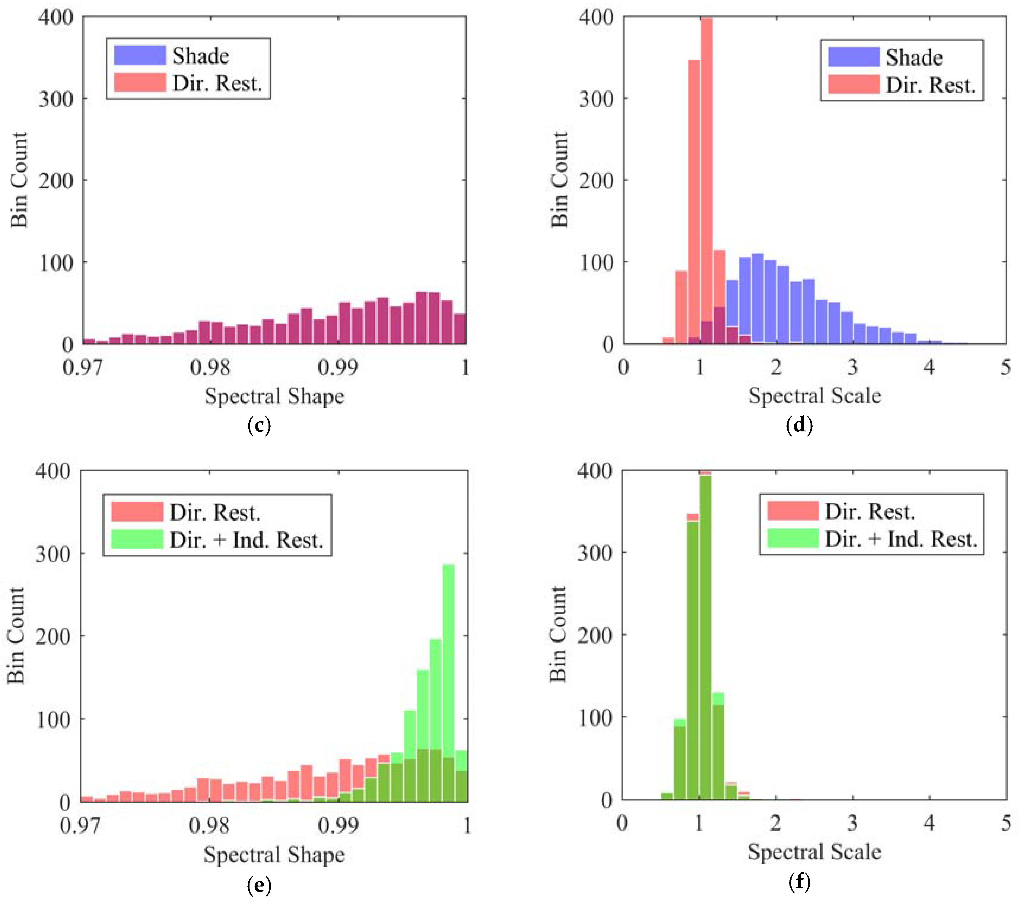
Figure 10.
Band correlation of the original partially shaded HSI, indirectly restored HSI, directly scaled HSI, and indirect restoration applied to a directly scaled HSI. Note the band correlation results are clipped at ~1800 nm due to insufficient signal in the reference full shade image.
Figure 10.
Band correlation of the original partially shaded HSI, indirectly restored HSI, directly scaled HSI, and indirect restoration applied to a directly scaled HSI. Note the band correlation results are clipped at ~1800 nm due to insufficient signal in the reference full shade image.

Figure 11.
(a) Spectral shape; and (b) spectral scale median versus number of direct adjustment wavelengths, limited to commercially available lidar wavelengths.
Figure 11.
(a) Spectral shape; and (b) spectral scale median versus number of direct adjustment wavelengths, limited to commercially available lidar wavelengths.

Figure 12.
Comparison of direct scale and direct shift spectrum adjustments using: (a) two; and (b) three wavelength locations.
Figure 12.
Comparison of direct scale and direct shift spectrum adjustments using: (a) two; and (b) three wavelength locations.

Figure 13.
(a) Spectral shape; and (b) spectral scale median metrics as a function of an increasing number of uniformly spaced direct adjustment wavelength locations.
Figure 13.
(a) Spectral shape; and (b) spectral scale median metrics as a function of an increasing number of uniformly spaced direct adjustment wavelength locations.


Table 1.
Terrestrial laser scanner and hyperspectral camera specifications.
| TLS: Riegl VZ-400 | HSI: Spectral Imaging, Ltd. Spectral Camera SWIR | ||
|---|---|---|---|
| Property | Value | Property | Value |
| Laser wavelength | 1550 nm | Wavelength range | 970–2500 nm |
| Beam divergence | 0.35 mrad | Spectral pixel count | 240 |
| Maximum range | 400 m | Spectral sampling | 6.3 nm/pixel |
| Pulse repetition | 300 kHz | Spatial pixel count | 320 |
| Range accuracy | 5 mm at 100 m | Camera output | 14 bit |
| Lens focal length | 22.5 mm | ||
© 2017 by the authors. Licensee MDPI, Basel, Switzerland. This article is an open access article distributed under the terms and conditions of the Creative Commons Attribution (CC BY) license (http://creativecommons.org/licenses/by/4.0/).
Share and Cite
MDPI and ACS Style
Hartzell, P.; Glennie, C.; Khan, S. Terrestrial Hyperspectral Image Shadow Restoration through Lidar Fusion. Remote Sens. 2017, 9, 421. https://doi.org/10.3390/rs9050421
AMA Style
Hartzell P, Glennie C, Khan S. Terrestrial Hyperspectral Image Shadow Restoration through Lidar Fusion. Remote Sensing. 2017; 9(5):421. https://doi.org/10.3390/rs9050421
Chicago/Turabian StyleHartzell, Preston, Craig Glennie, and Shuhab Khan. 2017. "Terrestrial Hyperspectral Image Shadow Restoration through Lidar Fusion" Remote Sensing 9, no. 5: 421. https://doi.org/10.3390/rs9050421
Note that from the first issue of 2016, this journal uses article numbers instead of page numbers. See further details here.