Article

Sea Surface Currents Estimated from Spaceborne Infrared Images Validated against Reanalysis Data and Drifters in the Mediterranean Sea

by
Céline Heuzé
1,*,
Gisela K. Carvajal
2,
Leif E. B. Eriksson
2 and
Monika Soja-Woźniak
2,3
1
Department of Marine Sciences, University of Gothenburg, 405 30 Gothenburg, Sweden
2
Department of Earth and Space Sciences, Chalmers University of Technology, 412 58 Gothenburg, Sweden
3
CSIRO Commonwealth Scientific and Industrial Research Organisation, Oceans and Atmosphere, 7004 Hobart, Australia
*
Author to whom correspondence should be addressed.
Remote Sens. 2017, 9(5), 422; https://doi.org/10.3390/rs9050422
Submission received: 14 March 2017 / Revised: 19 April 2017 / Accepted: 27 April 2017 / Published: 29 April 2017

Abstract

:
Near-real time sea surface current information is needed for ocean operations. On a global scale, only satellites can provide such measurements. This can be done with data from infrared radiometers, available on several satellites, thus giving several images a day. This work analyses the accuracy of such an estimation of surface current fields retrieved with the maximum cross correlation (MCC) method, here used to track patterns of Advanced Very High Resolution Radiometer (AVHRR) brightness temperature between 224 pairs of consecutive images taken between January and December 2015 in the western Mediterranean Sea. Comparison with in-situ drifters shows that relatively small patterns, moving at a slow speed, tracked between images separated by less than four hours give the best agreement. The agreement was strongest in summer, and consistent with low wind, non-eddying situations. When compared to a daily reanalysis field, the averaged satellite-retrieved fields showed good agreement, but not the in-situ drifter data. Drifter data should hence be used to complement satellite-retrieved currents rather than to validate them, since they may measure different components of the surface currents.

Graphical Abstract

1. Introduction

Near-real time measurements of sea surface currents are required, for example, for oil spill or other pollution confinement [1,2] and search and rescue missions [3]. These measurements would also make navigation more comfortable and fuel-efficient, thanks to adequate re-routing [4]. However, the in-situ monitoring of currents using surface drifters is not feasible over large regions. Remote sensing is hence a relevant alternative.
Remote sensing of ocean surface currents can be based on HF (3–30 MHz) [5] or X band (8–12 GHz) coastal radars [6]. In the open ocean, surface currents can be measured by radars aboard ships [7]. For large-scale global measurements, however, satellites are needed. Using satellites, weekly geostrophic currents can be estimated by altimetry [8]. For non-geostrophic currents and/or when a higher temporal resolution is required, a common method consists of tracking the movement of patterns of ocean colour or sea surface temperature [9,10,11,12]. This is what we do in this manuscript.
Both the technology and the methods for retrieving sea surface currents from sea surface temperature are more than thirty years old [9]. However, this process has still not been automated for near-real time retrievals, probably because validation studies are too few, limited to a small region or time period [9,11,13,14]. Models can be used to artificially create long time series of data for comparisons over a large region [10,15,16], but these are often not realistic enough to guarantee that the method will still work when applied to real—sometimes cloud-covered—images [17].
The western Mediterranean Sea is a region that seems well-suited for a validation study of the current retrieval. It has a high concentration of in-situ drifters [18], and is sunny enough to ensure many cloud-free days. However, it is also a challenging region for the retrieval, since it features many oceanic eddies [19,20] and has strong seasonal differences in its current and wind regimes [21]. The aim of the present study is to assess whether near-real time ocean current retrieval using spaceborne infrared images would be feasible year-round in such a complex ocean current region.
Here we test the retrieval of sea surface currents using one year of infrared images of sea surface temperature in the western Mediterranean Sea compared to in-situ surface drifters. We first perform a sensitivity study to determine the best settings of the algorithm, then study if the accuracy of the retrieval is linked to properties of the images, before concluding by comparing both drifters and retrieved velocity to reanalysis data.

2. Data and Methods

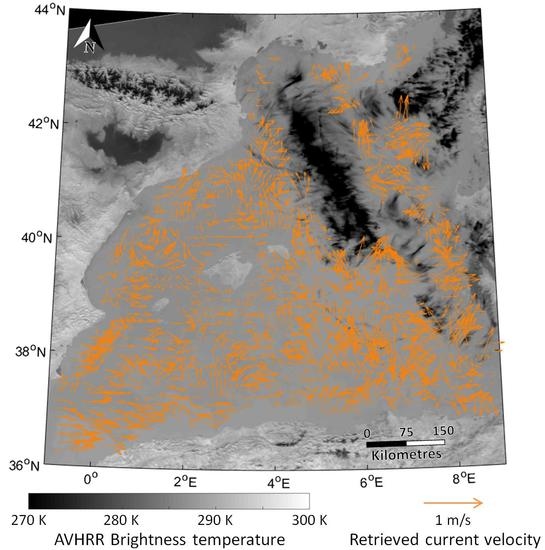
2.1. Satellite, Drifter, and Reanalysis Data

This study uses brightness temperature data at 10.8 μ m (black body temperature for channel 4) acquired by the Advanced Very High Resolution Radiometer (AVHRR). The AVHRR instrument flies on several satellites operated by NOAA and Eumetsat (MetOp-A and MetOp-B). Level 1b products were downloaded from the comprehensive large array-data stewardship system (CLASS) with the 1 km pixel resolution. Before running the retrieval algorithm, the data were reprojected using the BEAM software provided by the European Space Agency.
We used 224 pairs of images from 1 January to 31 December 2015 covering at least part of the western Mediterranean Sea (latitudes 36 N to 44 N, longitudes 1 E to 9 E). This area was selected due to the large overlap with data acquired by in-situ instruments, as described below. The satellite images were selected after a first visual assessment, eliminating the images that were mostly cloud-covered and/or which included less than a quarter of our area of interest.
In-situ ocean surface current data that are compared to the retrieved currents were obtained from the MyOcean data portal (http://www.myocean.eu/) of the Copernicus Marine Environment Monitoring Service (CMEMS). We make use of the “Mediterranean Sea near-real time observations” dataset (product identifier INSITU_MED_NRT_OBSERVATIONS_013_035, last accessed in February 2016) from January to December 2015. The data are automatically quality-controlled and are made available within 24–48 h from acquisition, on average (more information on http://marine.copernicus.eu). We considered only those drifters whose data were at the sea surface or at a depth strictly shallower than 1 m. All drifters used in this study are undrogued.
Finally, a second point of comparison is provided by the “Mediterranean Sea Physics Analysis and Forecast” product of CMEMS (product identifier MEDSEA_ANALYSIS_FORECAST_PHYS_006_001). It consists of daily mean sea surface current velocity fields at a 7 km horizontal resolution. This product is a coupled hydrodynamic (NEMO, [22])—wave (WaveWatch-III, [23]) model, whose outputs are corrected daily by the assimilation of temperature and salinity profiles as well as along-track sea level anomaly observations [24].

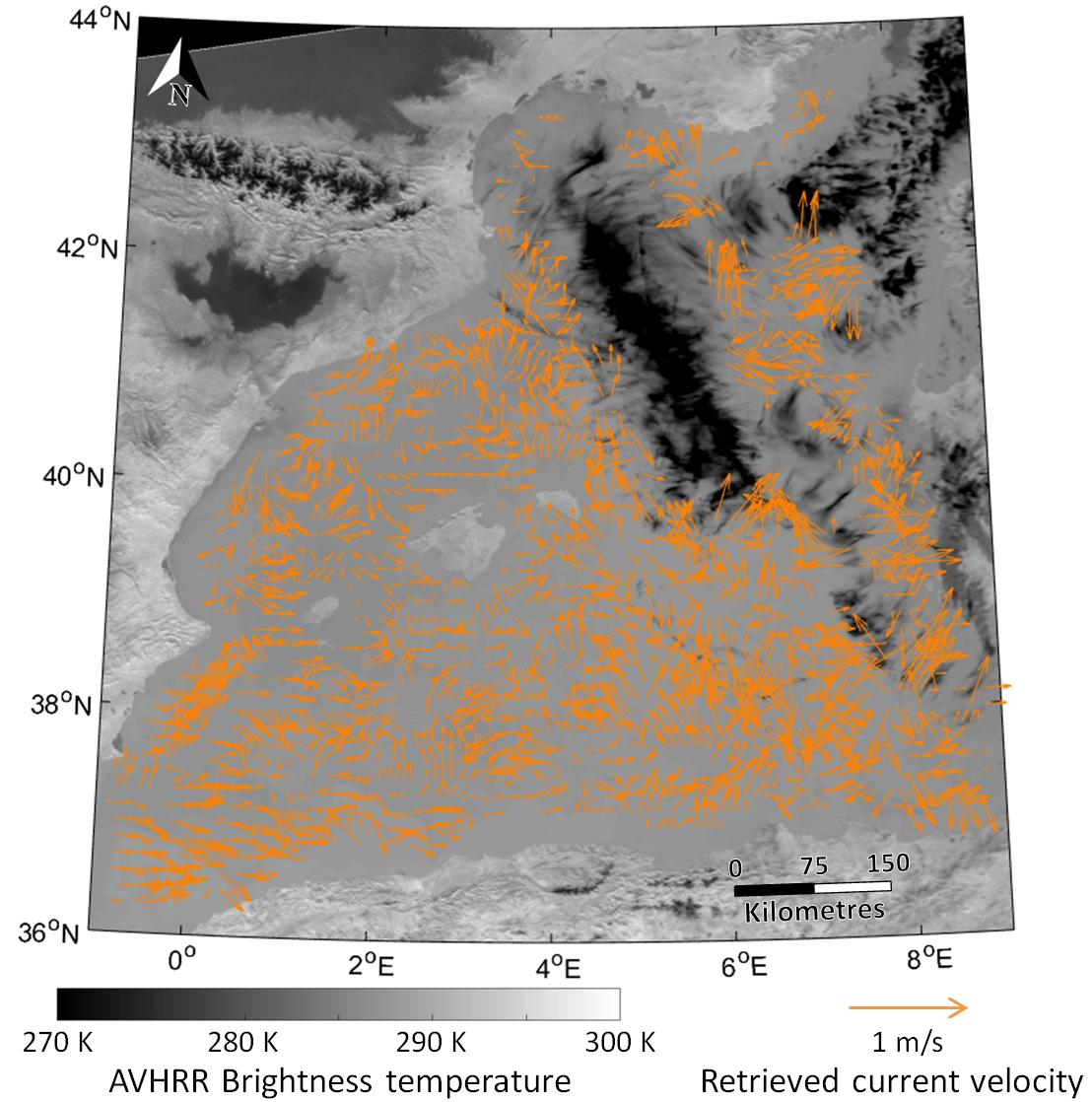
2.2. Sea Surface Current Retrieval with the Maximum Cross Correlation Algorithm

Sea surface currents are retrieved from the brightness temperature images using the maximum cross correlation (MCC) method [9]. Sea surface temperature patterns are tracked from one image to the next, and the displacement of these patterns over the time interval between the two consecutive images gives the current velocity. In practice, the first image is subdivided in “templates”. For each of these templates, the temperature field is compared to that of the same region in the second image, region augmented by a specific area (this forms the “search window”). The returned velocity is the one corresponding to the maximum correlation between the template and the search window.
When using the MCC, three settings have to be chosen, whose effect on the accuracy of the results is studied in Section 3.1:
  • the size of the template, that we here define as a box of 5, 10 (default), or 20 km per side;
  • the size of the search window, here defined by setting the maximum velocity that the retrieved field cannot exceed to 1.0 m s 1 (default), 1.3 m s 1 , or 1.8 m s 1 ;
  • the maximum cross-correlation threshold, which means that velocity values are returned only if the maximum correlation is larger than 0.3, 0.6 (default), or 0.9.
Prior to using the MCC, the land is masked out using coastline data from the Global Self-consistent Hierarchical High-resolution Shorelines dataset (GSHHS, [25]). To avoid any shadowing effect from the coast, we considered only data further than half a search window away from the coast. Due to the different scales in brightness temperature inherent to each image, the brightness temperatures were then normalized, and clouds were detected (and subsequently ignored by the algorithm) as having a normalized brightness temperature lower than minus one. This criteria was validated by careful visual verification. To be able to measure current speeds lower than 1 m s 1 without considering effects of diurnal variability and mixing, calculations were performed only if the pair of images were separated by two to seven hours (e.g., [10,15]).

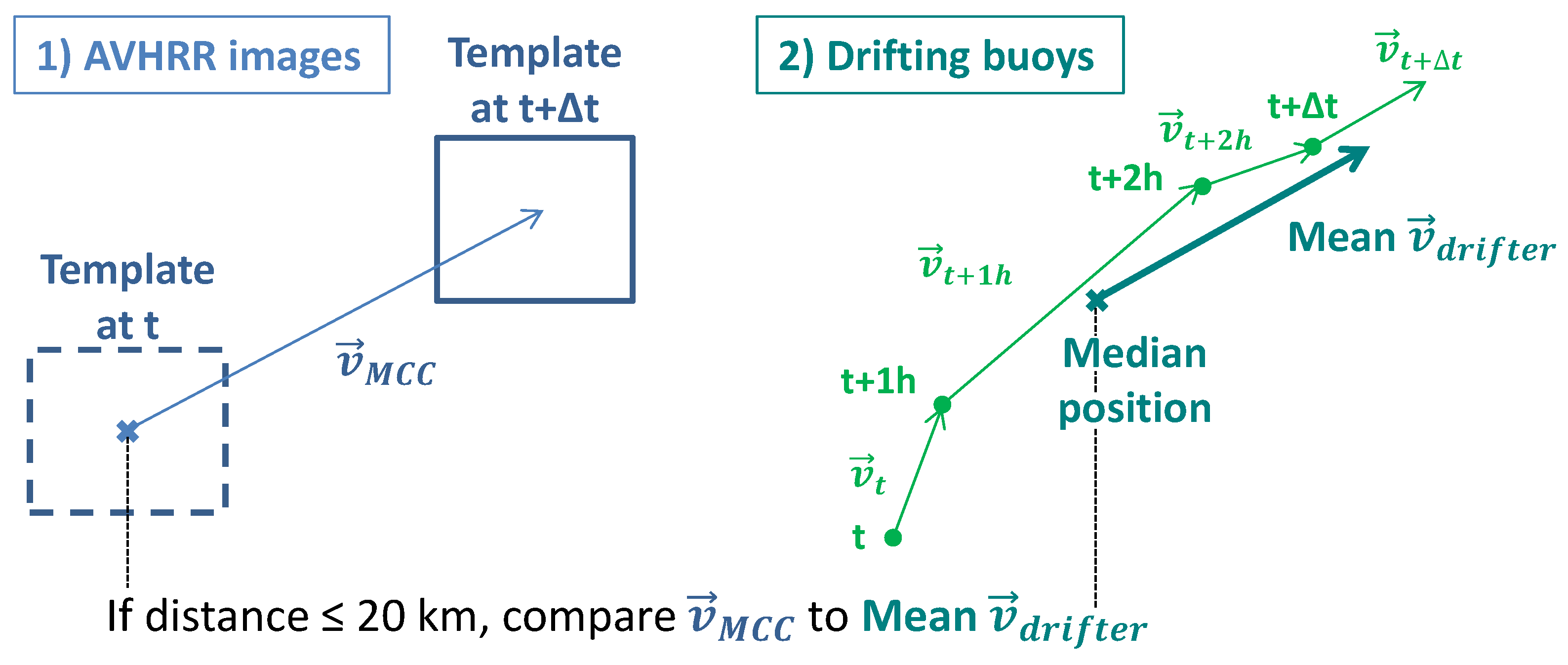
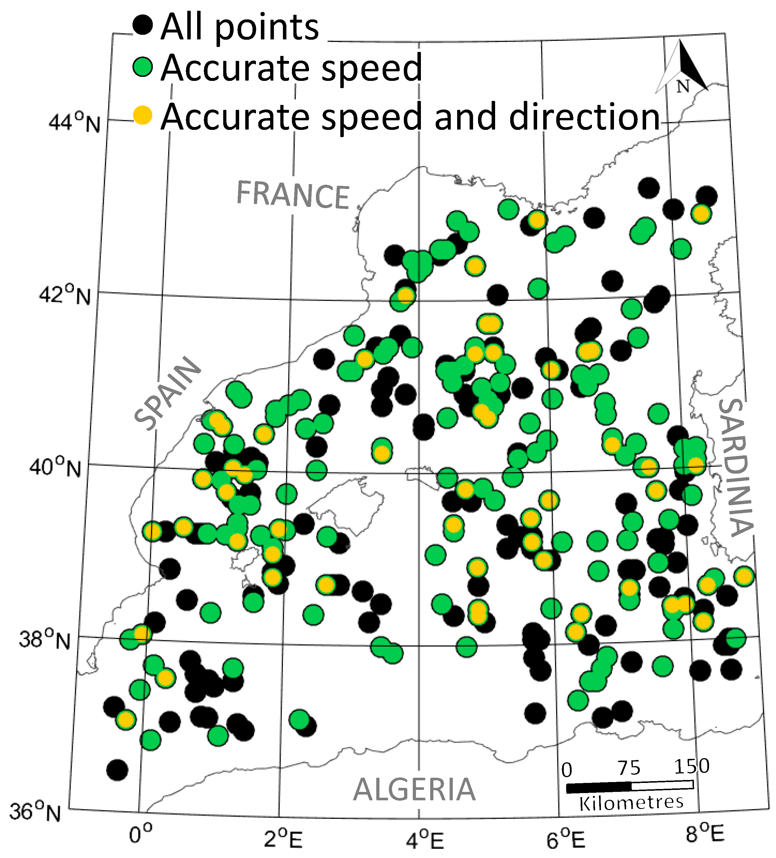
2.3. Methods for Comparison

We validate the sea surface current retrieval by comparing it first to the in-situ drifter data. This is a point-by-point comparison between the MCC results of each pair of images and the drifters with measurements during the same time interval as the pair of images. We define the drifter velocity as the mean over all the successive positions of the drifter divided by the time interval, and return it at the median position of the drifter over the time interval (Figure 1, right).
We perform a three-step filtering on the 2178 points of comparison that were returned between 1 January and 31 December 2015:
  • we discard both MCC and drifter points with a speed equal to zero, for which a direction cannot be estimated;
  • we discard the MCC points that are further than 20 km away from a drifter (Figure 1). We tested different thresholds between 10 and 50 km, and found that the results were not significantly affected by this choice of threshold;
  • we discard the MCC points that are within 20 km of each other and whose directions differ by more than 90 . For such points, the uncertainty attached to the MCC result is so high that an agreement with in-situ observation is meaningless (and due to luck).
We test the accuracy of the retrieval when compared to the drifter data on the points that are left after this filtering. In agreement with, for example, Bowen et al. [14] or Warren et al. [11], we consider that the retrieval is accurate enough if the error (MCC - drifter) in speed is lower than 0.2 m s 1 and the error in direction lower than 45 . In a real-life situation, such criteria would ensure the correct definition of a search or work area.
We then compare the MCC velocity fields and drifter values to the daily mean reanalysis. To do so, we average all the results returned by the MCC and all the drifters’ positions over 24 h. In practice, the MCC average consists of the results from one to six pairs of images, usually between 9.00 and 21.00 UTC (i.e., 10.00 and 22.00 local time), whereas the drifter average has 24 h values. We interpolate the MCC fields onto the reanalysis horizontal grid so that we can look at differences between the two fields.

3. Results and Discussion

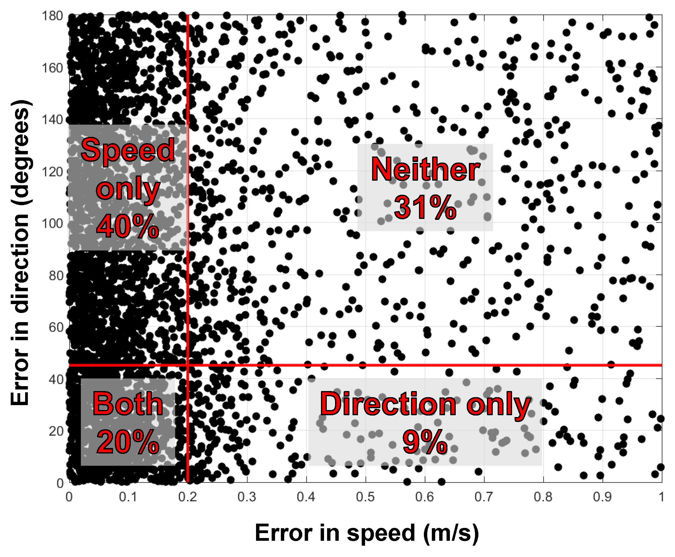
3.1. MCC Performance—Sensitivity Experiment

We first determine which settings of the MCC algorithm produce the largest agreement in terms of data volume. The most accurate settings hence defined will be kept and further used in the rest of the manuscript.
We assess the influence of the size of the template area, the size of the search window (i.e., the maximum velocity parameter), and the maximum correlation threshold on the accuracy of the MCC surface current retrievals. Only one of the three parameters is changed at a time, while the other two are set to the default values (template size of 10 km, maximum velocity of 1.0 m s 1 , and correlation of 0.6). We separately assess the accuracy of the methods in terms of speed and direction of the current field, as reported in Table 1.
Changing the template size produces the best results in terms of speed: 63% of the points have an accurate speed when compared to the in-situ drifters for a size of 5 km × 5 km (Table 1, second column). Increasing the template size results in less agreement in speed (45%); decreasing the size results in less agreement in direction (23%), so overall, the default experiment is the one with the most agreement in both speed and direction (Table 1—16% for the default experiment, 12% and 13% for 5 and 20 km, respectively). Moreover, the default experiment 10 km is the one with the most points of comparison. In the western Mediterranean Sea, 10 km seems to be the best compromise: too small a size, and the template has too low an entropy. The template must be large enough to feature clearly-defined fronts, since the MCC cannot return along-isotherm velocities [9]. In contrast, with too large a size, noise can dominate. In that region in particular, a template of 20 km per side or more can contain several vortices [20].
Enlarging the search window by increasing the maximum allowed speed should result in a better detection of the largest values and return more points than the default 1.0 m s 1 setting. In fact, here the accuracy in speed decreases as the maximum allowed velocity increases (Table 1: 56%, 45%, and 40% for 1.0, 1.3, and 1.8 m s 1 , respectively). This is because a small search window forces the algorithm to return small velocities, hence avoiding large outliers. The accuracy regarding the direction is slightly improved with the largest maximum velocity setting (30% instead of 28%), but the default setting remains the one with the largest agreement in both speed and direction. The total amount of points returned hardly increases with the maximum velocity settings tested here (from 351 to 353 and 359), hence the default setting of 1.0 m s 1 is preferable.
Finally, decreasing the maximum correlation threshold decreases the agreement in speed but increases the agreement in direction enough to perform slightly better than the default setting when considering both agreements (17% for R = 0.3, 16% for the default R = 0.6, Table 1). However, a lower correlation threshold means that more points that are returned have to be eliminated because we cannot trust them [9]. Increasing the correlation to R = 0.9 reduces the agreement when comparing the MCC retrievals to in-situ drifters. We shall come back to this result in Section 3.3.
The sensitivity study showed that the default settings:
  • template window of 10 km by 10 km;
  • maximum speed of 1.0 m s 1 ;
  • correlation threshold R = 0.6;
are the best compromise to obtain an agreement in speed and direction, but also the largest number of points of comparison. These results are consistent with other studies using the MCC algorithm. In the literature, the template window size is region specific: 10 km in Korea straits [11], 24 km by the California coast [26], 30 km in East Australia [14], 46 km in the Gulf Stream [27]. The maximum velocity of 1.0 m s 1 that we find to be most adapted is often chosen by other authors, regardless of the study area [14,26,27]. The value of the correlation cut-off is rarely indicated in other authors’ methodology; our value of 0.6 is in agreement with, for example, Bowen et al. (2002) [14].

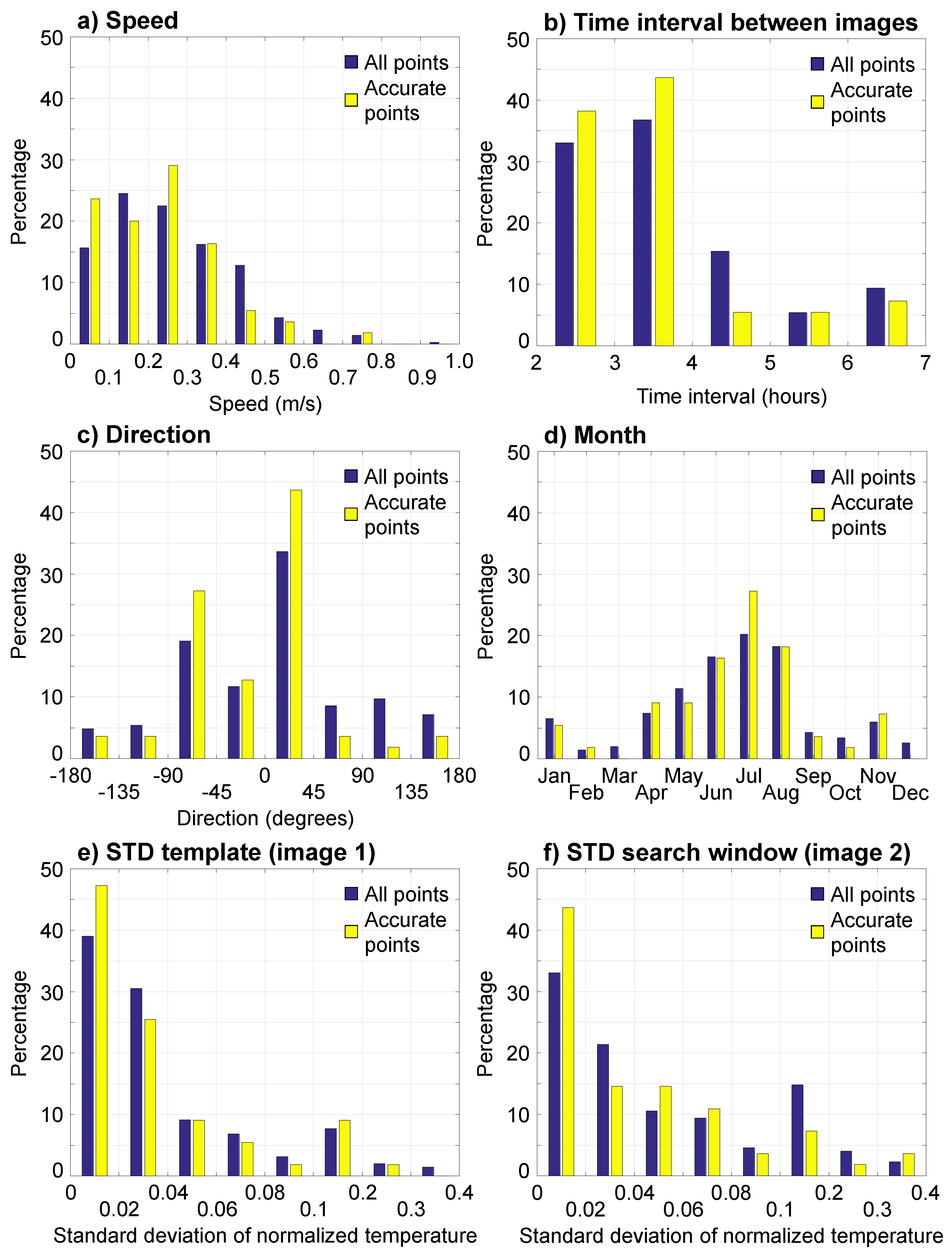
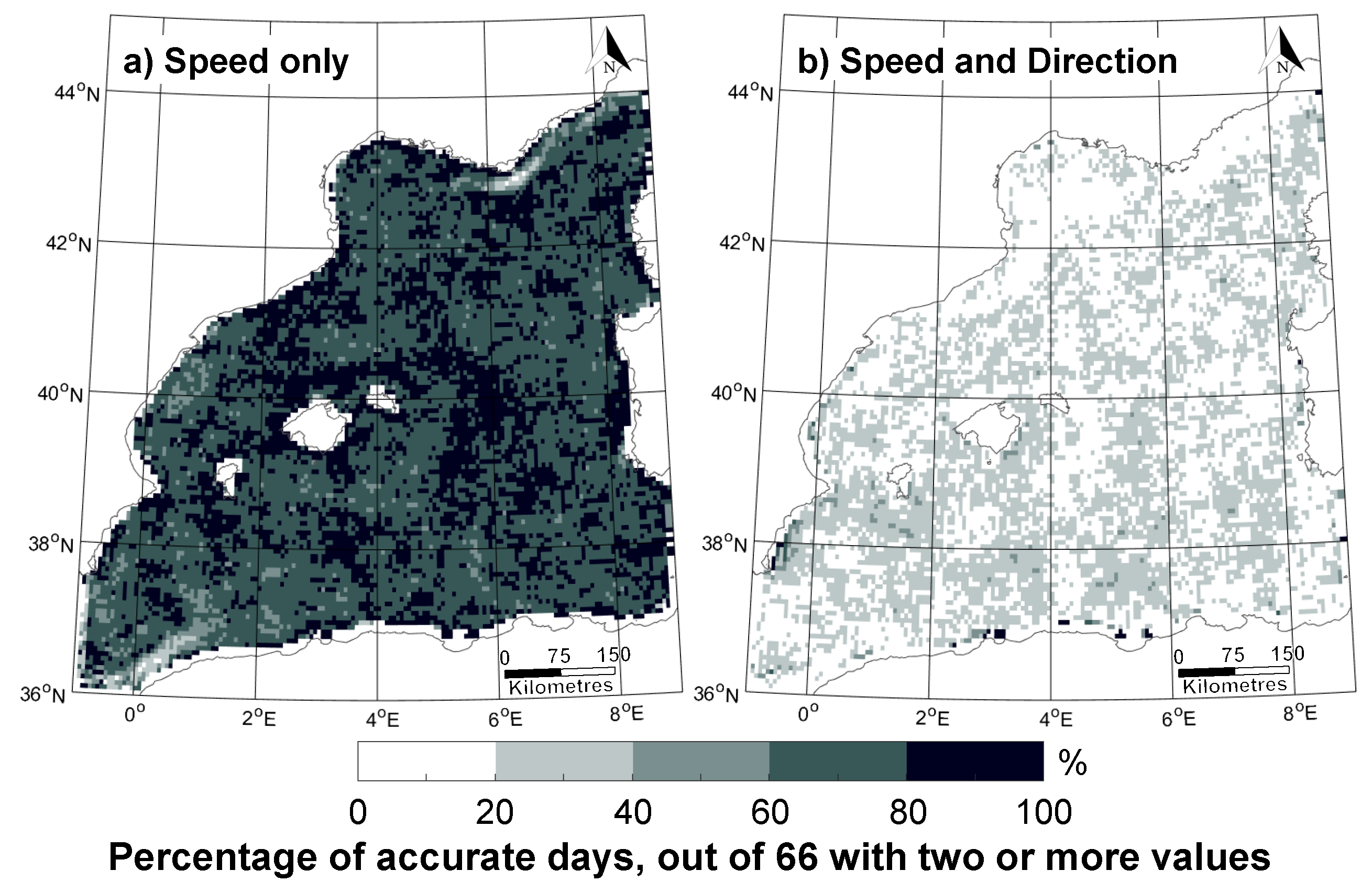
3.2. MCC Performance—Characteristics of the Images

Since the accuracy of the retrievals could not be dramatically improved by changing the settings, we now investigate if the accuracy could be linked to some physical parameters, using only the default settings. More precisely, can we find some characteristics of the pair of images that consistently return (in)accurate results when compared to the in-situ drifter data?
The first characteristic that we test is the location of the retrieval. Our study area covers approximately 500,000 km 2 of ocean and features distinct surface current patterns [19], yet the accurate points do not seem to be limited to a specific region (orange dots, Figure 2). They are also not consistently limited to a specific distance from the coast. For example, the Algerian coast to the south is data-poor, and mostly has points that are only accurate in speed (green dots, Figure 2). The Spanish coast to the west and the Sardinia coast to the east are data-rich and feature all types of points within a few kilometres from each other. Accurate points are encountered both in the open ocean and close to the coast.
One characteristic which matters for the retrieval’s accuracy is the retrieved velocity itself (Figure 3). Seventy-five percent of the accurate points have a speed lower than 0.3 m s 1 , compared to 63% of all the points tested (yellow bars compared to the dark blue bars, Figure 3a). Surprisingly, these low speeds are associated with a short time interval between the two images (Figure 3b). One would expect low speeds to be better detected over long time intervals, to give time for the patterns to have moved noticeably, but in fact 83% of the accurate points correspond to a time interval smaller than 4 h (Figure 3b). These two results—low speed and short time interval—suggest that it is the coherence of the pattern that matters (i.e., a pattern that has not yet been distorted by eddies). These particular values are probably specific to our region of study—the eddy-rich western Mediterranean Sea [19].
Two other crucial characteristics seem to be the direction of the retrieved sea surface current and the month during which the images were taken (Figure 3c,d). The accurate points tend to go north- and westward and be in summer. Note that assessing the relative error instead of using a threshold in absolute error returns a similar seasonal distribution (not shown). This result is consistent with circulation patterns, and in particular wind regimes in the western Mediterrean Sea [21]. In particular, the winds of winter are three times as strong as those of summer [21]. It is possible that surface drifters and satellite retrievals do not agree in winter because the undrogued drifters are more affected by the wind than the sea surface temperature patterns tracked by the MCC. It is also a known limitation of the MCC retrieval that the current to be retrieved must be solely advected, not rotated [9,14]; therefore, another possible explanation for the winter disagreement is that there are then too many mesoscale wind-induced eddies and vortices [19,20,21]. Moreover, it is possible that satellite image matching is more challenging in winter due to the lower amount of cloud-free images.
Finally, slightly counter-intuitively [9], the accurate points are significantly more associated with low standard deviation of the template (Figure 3e) and search window (Figure 3f) than the rest of the points. One would have expected clear patterns that strongly distinguish themselves from the ambient noise. In fact, a low standard deviation on the template (Figure 3e) again suggests that coherent patterns—fully contained by the template box—are most important. In the search window (Figure 3f), it is only normal to find the same values as in the template, especially for the accurate points.
In summary, the best agreement with the in-situ surface drifters is obtained by considering slow-moving coherent patterns, ideally in summer. However, since the undrogued drifters are so easily affected by the wind and waves, they may not be optimal for validation studies in windy regions or periods. We investigate this question in the following section, and compare both MCC-retrieved currents and drifter values to a daily reanalysis product.

3.3. MCC and Drifters vs. Reanalysis

So far in this manuscript, we have not validated the MCC-retrieved velocity fields. When compared to the in-situ drifter data, hardly one in five points agree for both speed and direction. However, most of the disagreement seems to be associated with eddy activity and/or winds. Can it simply be that drifters and satellites do not measure the same type of velocity? We check this by comparing both results to a third product: daily reanalysis velocity fields.
Quantitative estimates of the errors between the different sea surface current products (Table 2) suggest that the MCC is more similar to the reanalysis than to the drifters. In speed, the mean error and root mean squared error (RMSE) in speed are the lowest between MCC and reanalysis (0.08 and 0.19 m s 1 , respectively). The errors are largest in speed between drifter data and reanalysis, but lowest in direction. All three datasets have low mean errors in direction but large RMSE, indicative of occasional large errors. We now further assess the differences between MCC, drifter, and reanalysis separately.
First, we compare the MCC-retrieved fields to the reanalysis fields (Figure 4). The agreement in speed is very high. For the majority of the grid cells, more than 60% of the days with two retrievals or more are accurate, and over a third of the grid cells even exceed 80% (Figure 4a). For each day with two retrievals or more, the root mean squared error between the two fields is lower than 0.25 m s 1 . The agreement in both speed and direction exceeds 20% for more than two-thirds of the region, and even exceeds 60% locally (Figure 4b). This is a better result than the agreement between the MCC and the in-situ drifters (Table 1).
The point-by-point agreement between the in-situ drifters and the reanalysis is actually lower than that between the MCC and the reanalysis fields. Only 20% of the points agree in both speed and direction (Figure 5). The agreement in speed is satisfying (60%, Figure 5), but there is little agreement in direction (29%).
The imperfect agreement between the MCC-retrieved fields and the reanalysis daily velocities is not surprising. The reanalysis fields are daily averages of twenty-four-hourly values; the MCC fields are averages of two to six pairings of images, taken every two to seven hours between 9.00 and 21.00 UTC. However, the drifter points used in this section are also daily averages of twenty-four-hourly values. Our results further suggest that the undrogued drifters are probably most impacted by the Stokes, wind-induced surface velocity [28], and even waves. The MCC retrievals and the reanalysis also sense this wind-induced surface current [26], but mostly retrieve the mean advected surface velocity fields [9].

4. Summary, Limitations, and Conclusions

We retrieved surface currents in the western Mediterranean Sea from 1 January to 31 December 2015 by applying a maximum cross correlation algorithm to a series of infrared images of the ocean surface temperature measured by AVHRR. We assessed the performance of the MCC by comparing these retrievals to in-situ drifter and reanalysis data. We also tested the sensitivity of the MCC algorithm to three parameters that have to be set before any surface current retrieval:
  • the size of the template window, on the first image;
  • the maximum velocity allowed, which determines the size of the search window, on the second image;
  • the cutoff threshold in correlation.
We found that the best settings were a relatively small template window (which prevents the mixing of several patterns [20]) and a small search window, which controls the maximum speed that the current field can take and hence artificially prevents outliers (Table 1). However, even the best setting had a low agreement in both speed and direction with in-situ drifters (16% of the points). The agreement was not region-specific (Figure 2), but rather limited to summer, low-speed, coherent patterns (Figure 3). When compared to daily reanalyses, the satellite-retrieved fields show a better agreement (Figure 4) than the drifters (Figure 5). This suggests that the drifters are affected by the Stokes drift or small scale eddies (both of which are significant in the Mediterranean Sea [21]), whereas the reanalysis and satellite-retrieved values correspond mostly to the mean current.
The MCC method using AVHRR images is suitable for near-real-time ocean surface current retrieval, even in eddy-rich regions such as the Mediterranean Sea, provided there are cloud free images. One solution in cloudy areas can reside in retrieving currents with synthetic aperture radar (SAR) sensor instruments [29]. The thirty-year-long record of AVHRR infrared images can meanwhile be used to study the seasonal-to-multidecadal variability of the surface currents and to better constrain ocean models [30].

Acknowledgments

The main part of this work was funded by the Swedish National Space Board (Dnr. 167/14), with contributions from the European Union FP7 project SpaceNav (GA 607371). CH is funded by a VINNOVA Marie Curie fellowship (Dnr. 2015-01487). The authors would like to thank the three anonymous reviewers whose comments notably improved the quality of this paper.

Author Contributions

C.H., G.K.C. and L.E.B.E. conceived and designed the experiments; C.H. performed the experiments; all authors analyzed the results; G.K.C. wrote the MCC algorithm; M.S.-W. downloaded and processed the satellite images; C.H. and G.K.C. wrote the paper.

Conflicts of Interest

The authors declare no conflict of interest.

References

  1. Pisano, A.; De Dominicis, M.; Biamino, W.; Bignami, F.; Gherardi, S.; Colao, F.; Coppini, G.; Marullo, S.; Sprovieri, M.; Trivero, P.; et al. An oceanographic survey for oil spill monitoring and model forecasting validation using remote sensing and in situ data in the Mediterranean Sea. Deep Sea Res. 2016, 133, 132–145. [Google Scholar] [CrossRef]
  2. Eriksen, M.; Maximenko, N.; Thiel, M.; Cummins, A.; Lattin, G.; Wilson, S.; Hafner, J.; Zellers, A.; Rifman, S. Plastic pollution in the South Pacific subtropical gyre. Mar. Pollut. Bull. 2013, 68, 71–76. [Google Scholar] [CrossRef] [PubMed]
  3. Klemas, V. Remote Sensing of Coastal and Ocean Currents: An Overview. J. Coast. Res. 2012, 28, 576–586. [Google Scholar] [CrossRef]
  4. Ronen, D. The effect of oil price on containership speed and fleet size. J. Oper. Res. Soc. 2011, 62, 211–216. [Google Scholar] [CrossRef]
  5. Paduan, J.; Washburn, L. High-frequency radar observations of ocean surface currents. Annu. Rev. Mar. Sci. 2013, 5, 115–136. [Google Scholar] [CrossRef] [PubMed]
  6. Hessner, K.; Reichert, K.; Borge, J.; Stevens, C.; Smith, M. High-resolution X-Band radar measurements of currents, bathymetry and sea state in highly inhomogeneous coastal areas. Ocean Dyn. 2014, 64, 989–998. [Google Scholar] [CrossRef]
  7. Lund, B.; Graber, H.; Hessner, K.; Williams, N. On shipboard marine X-band radar near-surface current “Calibration”. J. Atmos. Ocean. Technol. 2015, 32, 1928–1944. [Google Scholar] [CrossRef]
  8. Wunsch, C.; Gaposchkin, E. On using satellite altimetry to determine the general circulation of the oceans with application to geoid improvement. Rev. Geophys. 1980, 18, 725–745. [Google Scholar] [CrossRef]
  9. Emery, W.J.; Thomas, A.C.; Collins, M.J.; Crawford, W.R.; Mackas, D.L. An objective method for computing advective surface velocities from sequential infrared satellite images. J. Geophys. Res. Oceans 1986, 91, 12865–12878. [Google Scholar] [CrossRef]
  10. Tokmakian, R.; Strub, P.T.; McClean-Padman, J. Evaluation of the maximum cross–correlation method of estimating sea surface velocities from sequential satellite images. J. Atmos. Ocean Technol. 1990, 7, 852–865. [Google Scholar] [CrossRef]
  11. Warren, M.A.; Quartly, G.D.; Shutler, J.D.; Miller, P.I.; Yoshikawa, Y. Estimation of ocean surface currents from maximum cross correlation applied to GOCI geostationary satellite remote sensing data over the Tsushima (Korea) Straits. J. Geophys. Res. Oceans 2016, 121, 6993–7009. [Google Scholar] [CrossRef]
  12. Shutler, J.D.; Quartly, G.D.; Donlon, C.J.; Sathyendranath, S.; Platt, T.; Chapron, B.; Johannessen, J.A.; Girard-Ardhuin, F.; Nightingale, P.D.; Woolf, D.K.; et al. Progress in satellite remote sensing for studying physical processes at the ocean surface and its borders with the atmosphere and sea ice. Prog. Phys. Geogr. 2016, 40, 215–246. [Google Scholar] [CrossRef]
  13. Emery, W.J.; Fowler, C.; Clayson, C.A. Satellite-image-derived Gulf Stream currents compared with numerical model results. J. Atmos. Ocean Technol. 1992, 9, 286–304. [Google Scholar] [CrossRef]
  14. Bowen, M.M.; Emery, W.J.; Wilkin, J.L.; Tildesly, P.C.; Barton, I.J.; Knewtson, R. Extracting multiyear surface currents from sequential thermal imagery using the maximum cross-correlation technique. J. Atmos. Ocean Technol. 2002, 19, 1665–1676. [Google Scholar] [CrossRef]
  15. Wahl, D.D.; Simpson, J.J. Physical processes affecting the objective determination of near surface velocity from satellite data. J. Geophys. Res. Oceans 1990, 95, 13511–13528. [Google Scholar] [CrossRef]
  16. Heuzé, C.; Carvajal, G.K.; Eriksson, L.E.B. Optimisation of sea surface current retrieval using a maximum cross correlation technique on modelled sea surface temperature. J. Atmos. Ocean Technol. 2017. submitted. [Google Scholar]
  17. Doronzo, B.; Taddei, S.; Brandini, C.; Fattorini, M. Extensive analysis of potentialities and limitations of a maximum cross-correlation technique for surface circulation by using realistic ocean model simulations. Ocean Dyn. 2015, 65, 1183–1198. [Google Scholar] [CrossRef]
  18. Holloway, G.; Nguyen, A.; Wang, Z. Oceans and ocean models as seen by current meters. J. Geophys. Res. Oceans 2011, 116, C00D08. [Google Scholar] [CrossRef]
  19. Millot, C. Circulation in the western Mediterranean Sea. J. Mar. Sys. 1999, 20, 423–442. [Google Scholar] [CrossRef]
  20. Isern-Fontanet, J.; García-Ladona, E.; Font, J. Vortices of the Mediterranean Sea: An altimetric perspective. J. Phys. Ocean. 2006, 36, 87–103. [Google Scholar] [CrossRef]
  21. Pinardi, N.; Masetti, E. Variability of the large scale general circulation of the Mediterranean Sea from observations and modelling: A review. Palaeogeogr. Palaeoclimatol. Palaeoecol. 2000, 158, 153–173. [Google Scholar] [CrossRef]
  22. Madec, G. NEMO Ocean General Circulation Model Reference Manuel; Technical Report; LODYC/IPSL: Paris, France, 2008. [Google Scholar]
  23. Tolman, H.L. User Manual and System Documentation of WAVEWATCH III TM Version 3.14; Technical Report, MMAB Contribution 276; MMAB: College Park, MD, USA, 2009. [Google Scholar]
  24. Lecci, R.; Drudi, M.; Grandi, A.; Fratianni, C. PRODUCT USER MANUAL for Mediterranean Sea Physical Analysis and Forecasting Product MEDSEA_ANALYSIS_FORECAST_PHYS_006_001; EU Copernicus Marine Environment Monitoring Service: Vincennes, France, 2016. [Google Scholar]
  25. Wessel, P.; Smith, W. A global, self-consistent, hierarchical, high-resolution shoreline database. J. Geophys. Res. B Solid Earth 1996, 101, 8741–8743. [Google Scholar] [CrossRef]
  26. Matthews, D.K.; Emery, W.J. Velocity observations of the California Current derived from satellite imagery. J. Geophys. Res. Oceans 2009, 114, 2156–2202. [Google Scholar] [CrossRef]
  27. Chubb, S.R.; Mied, R.P.; Shen, C.Y.; Chen, W.; Evans, T.E.; Kohut, J. Ocean surface currents from AVHRR imagery: Comparison with land-based HF radar measurements. IEEE Trans. Geosci. Remote Sens. 2008, 46, 3647–3660. [Google Scholar] [CrossRef]
  28. Longuet-Higgins, M.S. On the transport of mass by time–varying ocean currents. Deep Sea Res. 1969, 16, 431–447. [Google Scholar] [CrossRef]
  29. Qazi, W.A.; Emery, W.J.; Fox-Kemper, B. Computing Ocean Surface Currents Over the Coastal California Current System Using 30–Min–Lag Sequential SAR Images. IEEE Trans. Geosci. Remote Sens. 2014, 52, 7559–7580. [Google Scholar] [CrossRef]
  30. Flato, G.; Marotzke, J.; Abiodun, B.; Braconnot, P.; Chou, S.C.; Collins, W.J.; Cox, P.; Driouech, F.; Emori, S.; Eyring, V.; et al. Evaluation of Climate Models. In Climate Change 2013: The Physical Science Basis. Contribution of Working Group I to the Fifth Assessment Report of the Intergovernmental Panel on Climate Change; Cambridge University Press: Cambridge, UK; New York, NY, USA, 2013. [Google Scholar]
Figure 1. Schematic illustration of the two methods to estimate ocean surface currents: (1) using the maximum cross correlation (MCC), determining the displacement of a template window between two consecutive Advanced Very High Resolution Radiometer (AVHRR) images separated by Δ t ; (2) using the drifters, averaging the hourly drifter velocities over Δ t .
Remotesensing 09 00422 g001
Figure 2. Map of the western Mediterranean region of this study showing all the points of comparison (black), the points with an error in speed lower than 0.2 m s 1 (green), and those who also have an error in direction lower than 45 (orange center).
Remotesensing 09 00422 g002
Figure 3. For all the points that are compared (dark blue) and the points accurate both in speed and direction only (yellow), histograms representing the split of these points (as a percentage) according to (a) the MCC speed; (b) the time interval between the two images used for the MCC; (c) the MCC direction; (d) the month when the images were taken; (e) the standard deviation of the normalized brightness temperature of the template; and (f) that of the search window. For all subpanels, the values have been divided into intervals so that each bar represents all values within that interval.
Remotesensing 09 00422 g003
Figure 4. Maps of the western Mediterranean Sea showing for each grid cell the percentage of days with more than two MCC values (total 66) which differ from the reanalysis values by (a) less than 0.2 m s 1 in speed, and also (b) less than 45 in direction.
Remotesensing 09 00422 g004
Figure 5. Absolute error in direction as a function of the absolute error in speed for the daily averages of the drifters compared to the nearest reanalysis grid cell (4026 points in total). Points with an error larger than 1 m s 1 (11%) not shown. Red numbers indicate the proportion of points with an error in speed lower than 0.2 m s 1 and an error in direction lower than 45 (20%), accurate in speed only (40%), in direction only (9%), and accurate neither in speed nor in direction (31%).
Remotesensing 09 00422 g005
Table 1. Percentage of points accurate in speed (error lower than 0.2 m s 1 ), in direction (error lower than 45 ), and accurate for both criteria, for all the sensitivity experiments: changing the template size from 10 to 5 and 20 km, changing the maximum velocity from 1.0 to 1.3 and 1.8 m s 1 , and changing the maximum correlation threshold from 0.6 to 0.3 and 0.9. The first column corresponds to the default experiment.
Template Size10 km5 km20 km10 km10 km10 km10 km
Maximum Velocity1.0 m s 1 1.0 m s 1 1.0 m s 1 1.3 m s 1 1.8 m s 1 1.0 m s 1 1.0 m s 1
CorrelationR = 0.6R = 0.6R = 0.6R = 0.6R = 0.6R = 0.3R = 0.9
Speed Only56%63%45%45%40%51%53%
Direction Only28%23%29%28%30%32%24%
Speed and Direction16%12%13%14%11%17%12%
Total Points351293176353359317337
Table 2. Mean error and root mean squared error (RMSE) between the datasets, calculated using all the points of comparison for each diagnostic.
MCC-drifterMCC-ReanalysisDrifter-Reanalysis
Speedmean 0.11 m s 1 0.08 m s 1 0.31 m s 1
RMSE0.51 m s 1 0.19 m s 1 1.09 m s 1
Directionmean 14 4 2
RMSE 103 100 98

