
Quantifying Sub-Pixel Surface Water Coverage in Urban Environments Using Low-Albedo Fraction from Landsat Imagery

1
Department of Geography and Spatial Information Techniques, 818 Fenghua Road, Ningbo University, Ningbo 315211, China
2
State Key Lab of Information Engineering in Surveying, Mapping and Remote Sensing, Wuhan University, Wuhan 430079, China
3
School of Computer, Wuhan University, Wuhan 430079, China
*
Author to whom correspondence should be addressed.
Remote Sens. 2017, 9(5), 428; https://doi.org/10.3390/rs9050428
Submission received: 14 February 2017
/
Revised: 8 April 2017
/
Accepted: 16 April 2017
/
Published: 1 May 2017
(This article belongs to the Special Issue Learning to Understand Remote Sensing Images)
Abstract
:The problem of mixed pixels negatively affects the delineation of accurate surface water in Landsat Imagery. Linear spectral unmixing has been demonstrated to be a powerful technique for extracting surface materials at a sub-pixel scale. Therefore, in this paper, we propose an innovative low albedo fraction (LAF) method based on the idea of unconstrained linear spectral unmixing. The LAF stands on the “High Albedo-Low Albedo-Vegetation” model of spectral unmixing analysis in urban environments, and investigates the urban surface water extraction problem with the low albedo fraction map. Three experiments are carefully designed using Landsat TM/ETM+ images on the three metropolises of Wuhan, Shanghai, and Guangzhou in China, and per-pixel and sub-pixel accuracies are estimated. The results are compared against extraction accuracies from three popular water extraction methods including the normalized difference water index (NDWI), modified normalized difference water index (MNDWI), and automated water extraction index (AWEI). Experimental results show that LAF achieves a better accuracy when extracting urban surface water than both MNDWI and AWEI do, especially in boundary mixed pixels. Moreover, the LAF has the smallest threshold variations among the three methods, and the fraction threshold of 1 is a proper choice for LAF to obtain good extraction results. Therefore, the LAF is a promising approach for extracting urban surface water coverage.
1. Introduction
Worldwide mass migration to urban areas results in the land use/cover changes, changes in climate and intensifying anthropogenic modifications to urban environments [1]. This directly brings about more unexpected variations in urban surface water, especially in external morphological features of the coverage. The urban surface water changes further impact relevant aquatic biodiversity, healthy human life and even urban ecological balance [2]. Urban surface water deficiencies would aggravate the urban heat island effect and disrupt the living environments of urban vegetation; conversely, surface water inundation would result in flooding and even high fatality because of associated waterborne diseases [3]. Therefore, figuring out the coverage of urban surface water is a crucial issue for urban environments.
Remote sensing is a powerful data source for acquiring prior and comprehensive knowledge of urban surface water [4,5]. It allows synoptic, permanent, and dynamic urban surface water monitoring and is clearly superior to conventional in-situ measurements [6,7]. Among current remote sensing sensors, Landsat sensors have the greatest reputation in urban monitoring because of its advantages in terms of free availability, and moderate spectral, temporal, and spatial resolutions. Therefore, in our study, we implement Landsat imagery to investigate the urban surface water coverage problem.
Many studies have previously reported urban surface water extraction achievements using Landsat images. Regular water extraction methods can be categorized into three main groups [8,9]: (1) thematic classification methods [10,11,12]; (2) single-band thresholding methods [13,14]; and (3) water index methods [15,16,17].
Thematic classification methods formulate urban surface water extraction into a regular binary unsupervised or supervised classification problem on urban land cover types, and select surface water as the exclusive thematic class for mapping [10]. The methods easily bring about low accuracy in areas where the background land cover includes low albedo surfaces, such as asphalt roads and building shadows in urban areas [11]. Moreover, they utilize a Boolean set to classify each pixel as either water or non-water, and fail to achieve the desired accuracy, especially at the water-land (i.e., non-water) interface [12]. Single-band thresholding methods select a single diagnostic spectral band from Landsat images (e.g., band 5 from TM/ETM+) and delineate the urban surface water coverage with a manually-defined threshold [18]. Accordingly, the subjectivity of the threshold selection can lead to an overestimated or underestimated result and, moreover, the extracted surface water is affected by shadow noise [16].
Different from the above two methods, water index methods combine two or more spectral bands using algebraic operations to enlarge the divergence between water and non-water areas. McFeeters proposed the normalized difference water index (NDWI) to delineate urban surface water. The NDWI is implemented with a ratio model using the green band (i.e., band 2) and the near-infrared band (i.e., band 4) from Landsat TM/ETM+ data [15]. An empirical value of 0 is set as the threshold for extracting surface water from the raw Landsat images, and pixels with positive NDWI values are regarded as belonging to surface water. Unfortunately, the obtained NDWI surface water suffers from noise in built-up areas, and the threshold of 0 always results in an over-estimation of the surface water [16]. Subsequently, Xu presented another surface water index called modified normalized difference water index (MNDWI) [16]. MNDWI improves NDWI by replacing the near-infrared band (i.e., band 4) with the middle-infrared band (i.e., band 5) from Landsat TM/ETM+ images. MNDWI reduces the built-up area noise in NDWI, and it performs better than NDWI in extracting urban surface water where built-up areas dominate in the image scene. Nevertheless, the threshold of MNDWI is difficult to estimate because of their scene-driven features, and the problem adversely impacts its realistic performance of MNDWI [8]. To address the instability of MNDWI, the automated water extraction index (AWEI) was presented by combining multi-band Landsat images (i.e., bands 2, 4, 5, and 7 of Landsat TM/ETM+ images) [9]. The AWEI argues that the threshold of 0 is a good initialization for urban surface water extraction in the method.
The above three types of methods greatly benefit the studies of urban surface water extraction. However, one big problem of mixed pixels still exists in the urban surface water extraction procedure when using moderate spatial resolution Landsat images. In particular, the problem becomes more pronounced when extracting accurate boundaries of surface water. A simple cause for this problem is that the scale of urban land cover is often smaller than the field of view in the Landsat TM/ETM+ sensor (30 m) [19,20]. Subsequently, a few sub-pixel classifiers were presented to handle the mixed pixel problem. Sethre proposed a sub-pixel classifier named analysis spectral analytical process (AASAP), which aimed to expand the regular classifier into the sub-pixel field to detect the size and shape of ponds [21]. The classifier focuses on sub-pixel wetlands or ponds and requires careful verifications when implemented in the case of urban water extraction. Sun optimized the training samples with mixed training samples and then combined them with the support vector machine (SVM) classifier to improve the urban surface water extraction results [22]. However, the scheme suffers from slow computational speed and complicated manual operations, which seriously restricts its real-word applications in other urban areas.
Spectral unmixing is an alternative technique that can be used to solve the mixed pixel problem encountered in urban environments. It can be classified into linear spectral unmixing (LSU) and nonlinear spectral unmixing (NLSU), according to different mathematical assumptions in mixing patterns of urban land covers in the study area [23]. Numerous applications exploit the powerful performance of LSU in converting spectral information into physical abundances of materials on the earth’s surface [23]. Previously, researchers have made some trials related to the surface water extraction problem using spectral unmixing. Zhou integrated a multiscale extraction scheme with spectral mixture analysis techniques to improve water extraction in urban environments from moderate spatial resolution satellite images [24]. The feature of this work is to adopt the multiscale scheme that conducts surface water extraction in multiscale local regions in order to refine the result. Xie combined the water index NDWI with LSU and proposed an automatic subpixel water mapping (ASWM) method to map urban surface water at the sub-pixel scale [25]. Pure water extracted from NDWI and water fractions of mixed water-land pixels estimated from LSU constitute the final urban surface water map. As distinct from previous research, we propose a low albedo fraction (LAF) method based on LSU to extract urban surface water from Landsat imagery. In comparison to all of the above methods, our LAF methods have three major advantages, in the following:
- (1)
- The LAF method stands on the H-L-V [23] (i.e., high albedo-low albedo-vegetation) spectral mixture analysis of urban surface reflectances, and investigates the urban surface water extraction problem with the low albedo fraction map. Accordingly, our idea is different from above water extraction methods, especially sub-pixel classifiers and spectral unmixing methods by Zhou [24] and Xie [25].
- (2)
- The LAF method implements a steady initial threshold at 1 and that significantly reduces the work of parameter tuning in LAF. By contrast, current spectral unmixing-based methods by Zhou and Xie could not provide a stable threshold for fraction segmentation. The water index methods also suffer from the unstable initial threshold problem. Therefore, the LAF is easier to implement in real-word applications than other methods, such as spectral unmixing methods and water index methods.
- (3)
- The LAF method obtains high extraction accuracies of urban surface water, and it significantly improves the accuracy of sub-pixel surface water extraction when compared against MNDWI and AWEI.
2. Test Sites and Datasets
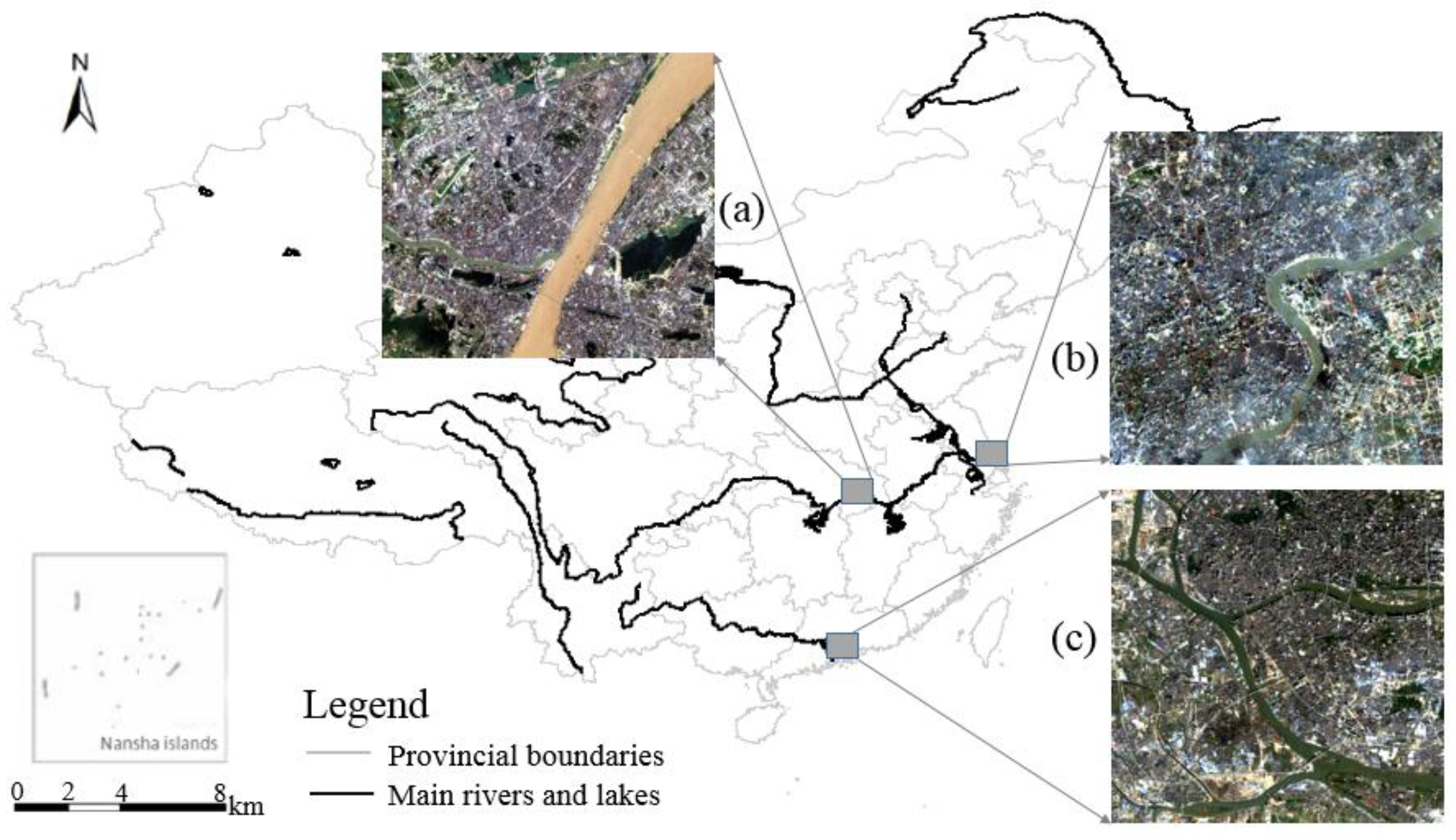
The test sites utilized in the study are located in three representative metropolises of China: Wuhan, Shanghai, and Guangzhou. Different surface features of the urban environments (e.g., different spatial patterns of land covers and different urban backgrounds) of the three sites render them good candidates for testing the proposed LAF method. The Wuhan metropolis lies in one of the fastest-growing regions in central China, and it is becoming a significant strategic center for the rejuvenation of the Chinese nation. Wuhan is centered at the confluence of the Yangzi River and Han River, as shown in Figure 1a. Shanghai is a famous international metropolis, and it is known for advanced economics, shipping, and finance. The Huangpu River in Figure 1b is very important for the health and wellbeing of people in Shanghai. Guangzhou is an important port in China. The Pearl River in Figure 1c runs around Guangzhou city, and is a vital source of drinking water. Figure 1 illustrates the different surface characteristics of all three metropolises, where it can be seen that they have similar land cover types, including built-up surfaces, tall buildings, rivers, and vegetation.
Landsat images of the three metropolises were acquired from the website of the United States Geological Survey (USGS) (available at http://www.glovis.usgs.gov) [26], and the subsets cover the main urban background types and surface water for extraction. The downloaded Landsat imagery belongs to a Level-1 precision- and terrain-corrected product (L1T). The utilized Landsat images are free of clouds in order to avoid any negative effects from cloud. A reference image was utilized to determine the ground truth of water pixels in Landsat images, and it greatly helped in evaluating the accuracies of extracted surface water, at either the pixel level or sub-pixel level. The original sources of the reference data were high spatial-resolution pan-sharpened Quickbird images from the Digital Globe Company, and the JPEG format image at 4m spatial resolution was exported from Google Earth Pro (available at www.google.com). We selected high spatial-resolution images (HSRI) with acquisition times as close as possible to the Landsat images, and tried our best to ensure that the land-cover classes of the Landsat images and the Google Earth images were the same for the same site. Table 1 lists detailed information about the reference data and Landsat images. Geo-referencing HSRI data with Landsat images was implemented to unify spatial references of the corresponding pixels in both datasets. The manual co-registration was carefully undertaken with a Root Mean Square Error (RMSE) of no more than 0.3 pixels, and 19 control points were manually selected from each image. The “true” boundaries of urban surface water at the test sites were manually digitized on screen from the reference data, and were then rasterized at 4 m spatial resolution.
3. Methodology
3.1. The Procedure of LAF Method
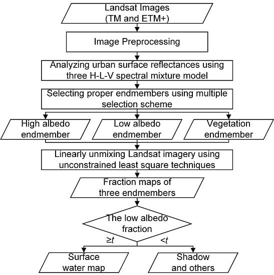
The LAF method explores the urban surface water extraction problem from the perspective of linear spectral unmixing and a three-endmember H-L-V (high albedo-low albedo-vegetation) model [23]. It extracts urban surface water coverage through threshold segmentation on the fraction map of the low albedo endmember. The overall procedure of extracting urban surface water using LAF is shown in Figure 2 and includes the following steps:
- (1)
- The Landsat images are preprocessed with radiometric calibration.
- (2)
- The three-endmember H-L-V linear mixture model is implemented to analyze surface reflectances of urban land cover types.
- (3)
- Endmembers covering high albedo, low albedo, and vegetation are carefully selected from Landsat images using our multiple selection scheme.
- (4)
- The unconstrained least square techniques are implemented to unmix Landsat images and to estimate the fractions of all three endmembers at each pixel. Fraction maps of all three endmembers are then obtained.
- (5)
- The binary classification is implemented to segment the fraction map of low albedo endmember, using a given threshold t. The pixels with low albedo fractions no less than t constitute the final surface water map of LAF.
3.1.1. Preprocessing of Landsat Images
Radiometric calibration is used to transform the initial digital numbers (DNs) in Landsat images into normalized exo-atmospheric reflectance. The procedure is implemented in ENVI 5.0 [27] with the input of calibrated parameters obtained from the header file of Landsat images. Atmospheric correction is not undertaken because previous studies have shown that the process has an unclear influence on fraction maps when image-based endmembers are used in the LSU method [28,29].
3.1.2. Analyzing Urban Surface Reflectances Using Three-Endmember H-L-V Model
Generally, the three-endmember vegetation-impervious surface-soil (V-I-S) model is utilized for urban landscape analysis from remote sensing data [30]. The model classifies urban land-cover classes into fraction combinations of vegetation, impervious surfaces, and soil; and its typical application is to extract urban vegetation [31]. The V-I-S model is, however, limited in urban surface water extraction because the idea of a single endmember could not represent the complicated land cover types in urban impervious surfaces. As a result, Wu and Murray (2003) separated impervious surfaces into high albedo and low albedo surfaces, and modified the V-I-S model into a four-endmember model [32]. The difference between the four-endmember model and the three-endmember H-L-V model is whether the model includes the soil endmember or not.
In contrast to previous works, we implement the three-endmember H-L-V model. Previous studies have demonstrated that the reflectance properties of land cover in urban environments can be accurately described as linear combinations of three endmembers of high albedo, low albedo and vegetation [33]. Moreover, the three-endmember H-L-V model avoids the misclassification of soil as high albedo that exists in the four-endmember model. Furthermore, our preliminary experimental results showed that the combination of the linear mixture model and H-L-V model is more suitable for urban surface water extraction. The three-endmember H-L-V linear mixture model is represented as follows [23]:
where is the spectral reflectance in band i, is the reflectance of endmember j in band i, is the fraction of endmember j, and is the bounded approximation error in the model.
3.1.3. Selecting Proper Endmembers Using a Multiple Selection Scheme
The result of endmember selection closely correlates with the success of the linear mixture model in urban surface water extraction. Moreover, a proper three-endmember H-L-V combination helps to robustly estimate a good threshold for extracting urban surface water from the fraction map of the low albedo endmember. In the study, we utilize a combination of different selection schemes to determine the three appropriate H-L-V endmembers from Landsat images. Multiple selection schemes combine the scatter plots of principal component analysis (PCA) transformation, image-based manual selection, and endmember optimization using cross-validation. The image-based selection scheme is adopted because of its advantages in terms of ease of operation and the same spectral response magnitude of selected endmembers with image spectra. The multiple selection schemes are implemented in the following procedures.
The first procedure is to implement PCA transformation to produce covariance-based principal component (PC) rotation and normalize the eigenvalues. The PCA transformation is implemented in ENVI 5.0 software with the input of Landsat images. For the H-L-V model, the two-dimensional normalized eigenvalue distributions of Landsat images could quantify the partitions of reflectance variance among all the PCs and formulate a triangular form with scatter plots of first two PCs [34]. The topology of triangular mixing space in Figure 3 is consistent with the mixing space of Landsat images. The pixels at the vertexes of the triangular topology correspond to high albedo, low albedo and vegetation endmembers [33]. The three vertex endmembers could accurately represent the most important physical properties of the surface reflectance of urban land cover types.
Meanwhile, because of the limits of spatial and spectral resolution in Landsat sensors, the Landsat images could not discriminate the wide variety of reflectances present in the urban environments. Accordingly, the three vertex endmembers in the triangular form might represent a variety of different ground objects and that might adversely impact the accuracy of estimates for pixels with the three endmember fractions. In particular, the high albedo endmember is the most compositionally variable and the least constrained by the triangular topology. Figure 3 illustrates that a wide variety of spectra exists near the high albedo vertex of the triangular topology of scatter plots. The fraction of the high albedo vertex endmember does not necessarily provide an accurate estimate of the overall albedo because of the non-linearity and dispersion of most mixing spaces near the high albedo vertex; that is, the high albedo vertex endmember in the triangular form could not accurately represent the wide variety of high albedo reflectances observed in the urban Landsat images. In contrast, the vegetation and low albedo endmembers are generally well constrained in the triangular topology. Therefore, the second procedure is to manually select endmembers from Landsat images, compare the endmembers with the vertex endmembers of the triangular form, and optimize the selection result via cross-validation.
The operation rules for three H-L-V endmembers via cross validation are listed in Table 2 and the technique details are as follows:
- (1)
- The low albedo endmember: The low-albedo endmembers correspond to deep dark shadow and water [29]. In this study, water is the most important object. Therefore, we chose the low albedo endmember from the deep dark water pixels, and the endmember has minimal brightness values in the image scene via cross-validation. The low albedo endmember is easy to determine from the image.
- (2)
- The vegetation endmember: The vegetation usually corresponds to grass or dense agriculture. The pixel with maximal normalized difference vegetation index (NDVI) values (dense grass and pasture) in the image scene is chosen as the vegetation endmember, using cross-validation. The vegetation endmember is also easily determined in the LAF method.
- (3)
- The high albedo endmember: The high albedo endmember shows much greater sensitivity to the selection method because it varies most greatly in amplitude within the triangular topology [29]. Therefore, we combine Landsat images with HSRI data to optimize the selection of the high albedo endmember via cross-validation. The initial high albedo endmembers are manually selected from building roofs, airport runways, and highway intersections in Landsat images, with reference to corresponding land covers in the HSRI data. Next, these initial endmembers are compared with the high-albedo vertex endmember in the scatter plots of PC1 and PC2. The endmember located closest to the high albedo vertex of the triangular topology is finally selected as the high albedo endmember [35].
3.1.4. Spectral Unmixing and Binary Classification of the Low Albedo Fraction Map
Spectral unmixing is utilized to solve the three-endmember H-L-V linear mixture model in Equation (1). Spectral unmixing was initially proposed for calculating land-cover fractions for a pixel [36]. The least square techniques are implemented to estimate the fraction of each endmember at each pixel by minimizing the model errors. The techniques can be grouped into unconstrained and constrained types. The differences between the two types are nonnegativity and sum-to-one constraints in the fractions of each pixel [37].
In the study, we implement the unconstrained least square techniques, for two reasons. The first is that the result of unconstrained least square techniques is only affected by the adopted model, and the second is that our objective is to explore the relations between urban surface water and the fraction map of low albedo endmember, and this purpose differs from current common applications of constrained least square techniques. After spectral unmixing operation with unconstrained least square techniques, the fractions of all three endmembers are estimated and the fraction maps are then obtained.
From the above analysis, the low albedo spectrum dominates in the pixels of urban surface water, and we accordingly extract them from the fraction map of the low albedo endmember. The binary map of urban surface water is achieved by segmenting the low albedo fraction map with a given threshold , shown as follows:
where is the fraction or abundance of the low albedo endmember in each pixel.
In LAF, we implement a cross-validation scheme to select an appropriate threshold. The scheme is initialized with a manually-defined threshold, and we then interactively estimate the sub-pixel accuracies (mentioned in Section 3.2) of urban surface water by tuning the threshold parameter from the initial value. Finally, we select an appropriate threshold with the optimal sub-pixel extraction accuracy that best balances over-estimation errors and under-estimation errors. It should be stressed that a good initialization is important for the above scheme. From our trial experiments, we found that, in the low albedo fraction map, pixels with fraction values clearly greater than 1 always belonged to water; pixels with fraction values around 1 were boundary mixed pixels dominated by water; and pixels with fraction values of less than 1 belonged to non-water. We also found that the pixels that were mixed by building shadows and other ground objects had fractions of the low albedo endmember smaller than 1. The shadows belong to non-water and their fractions do not affect the extraction result of LAF in urban surface water. Therefore, we manually select the initial threshold of LAF as 1, and implement the cross-validation scheme to achieve a proper binary classification map of urban surface water. The binary map after thresholding segmentation includes water and non-water, and the image is directly adopted as our final extraction result of urban surface without any filter operations, such as removing isolated or partial water pixels.
3.2. Accuracy Assessment Schemes on the Per-Pixel and Sub-Pixel Levels
Considering the fact that the MNDWI and AWEI obtain a better accuracy of urban surface water extraction than other current water extraction methods [8,9], the two methods are utilized to make comparisons with the proposed LAF. The thresholds in the three methods were estimated via cross-validation, and the best extraction results of urban surface water from all three methods were adopted for the comparison.
The per-pixel accuracy and sub-pixel accuracy were estimated from the binary map to evaluate the performance in extracting urban surface water. The per-pixel accuracy is to evaluate the overall performance of the LAF binary classification map, with pure pixels and boundary mixed pixels of surface water included. The ratio of spatial resolutions between the reference HSRI data and Landsat images is 4:30, meaning that one pixel in Landsat images corresponds to about 50 HSRI pixels. Similar to the idea expressed in [9], we regarded the pixels in Landsat imagery that consist predominantly of water (>50% proportions, i.e., over 25 HSRI pixels) as true water pixels, and vice versa. Using the random sampling scheme, the labels (water and non-water) of testing water pixels for overall per-pixel accuracy evaluation was manually digitized from Landsat imagery, and then compared with their true labels from reference data. The kappa coefficients (KC) were calculated and used to quantify the overall extraction accuracy of all three methods.
Different from overall per-pixel accuracy, the sub-pixel accuracy is to testify the specific performance of all three methods in extracting water from mixed pixels, especially from boundary pixels. The sub-pixel accuracy evaluation implemented the following four main steps.
- (1)
- The actual water fractions of testing boundary pixels were manually estimated via the visual overlay analysis of reference data and Landsat images. By overlaying the binary maps of extracted surface water from all three methods (AWEI, MNDWI and LAF) with the HSRI data, the water fraction of each boundary pixel from each method can be calculated. This was equal to the percentages of water pixels in the total number of HSRI pixels that were fully contained within the area of one pixel of Landsat imagery. For example, within the scene of one pixel from Landsat imagery, if the water occupies 20 of the total 50 HSRI pixels, the water fraction of the targeted boundary pixel is 40%. The process is repeated and the actual water fractions of all testing boundary pixels resulting from the three methods were achieved.
- (2)
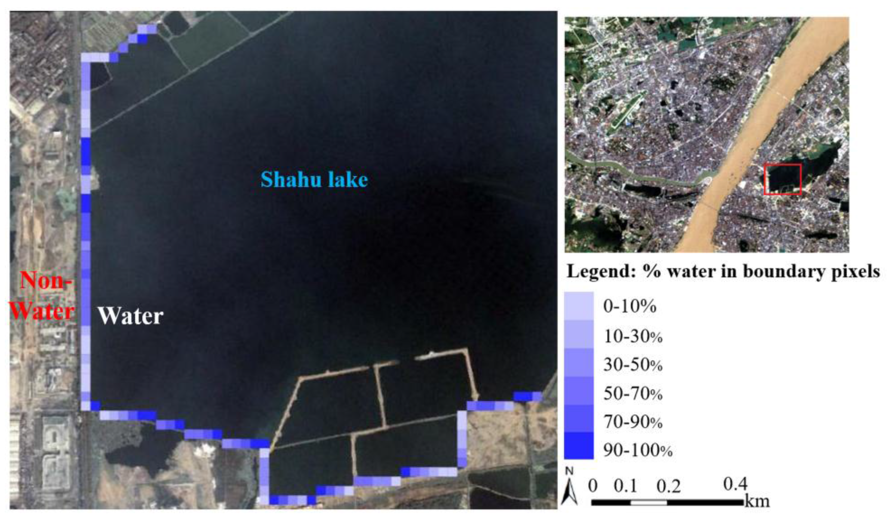
- The testing boundary pixels were designated into six categories according to their true water fractions. The true water fractions of all testing boundary pixels in the HSRI data can be classified into six categories, 0–10%, 10–30%, 30–50%, 50–70%, 70–90% and 90–100%. For example, Figure 4 shows six categories of true water proportions in the testing boundary pixels of Shahu lake, and the number of testing boundary water pixels is 106.
- (3)
- The estimation errors (EEs) of all three methods on each testing boundary pixel were estimated. The EEs for each testing boundary pixels at the sub-pixel level are the summation of over-estimation error and under-estimation error, defined according to the following two conditions: (a) if a testing boundary pixel in the binary classification map of each method was classified as water, its complement of the true water fraction is regarded as the sub-pixel over-estimation error; (b) in contrast, if the pixel was classified as non-water, its true water fraction is quantified as the under-estimation error at the sub-pixel level.
- (4)
- The average estimation errors (AEEs) in all six categories of testing boundary pixels were calculated and the set of AEEs with six elements for all three methods were obtained to quantify the sub-pixel water extraction accuracy of boundary mixed pixels at different water proportions.
4. Experimental Results and Analysis
4.1. Water Extraction Maps and Per-Pixel Accuracy Assessment in Overall Result
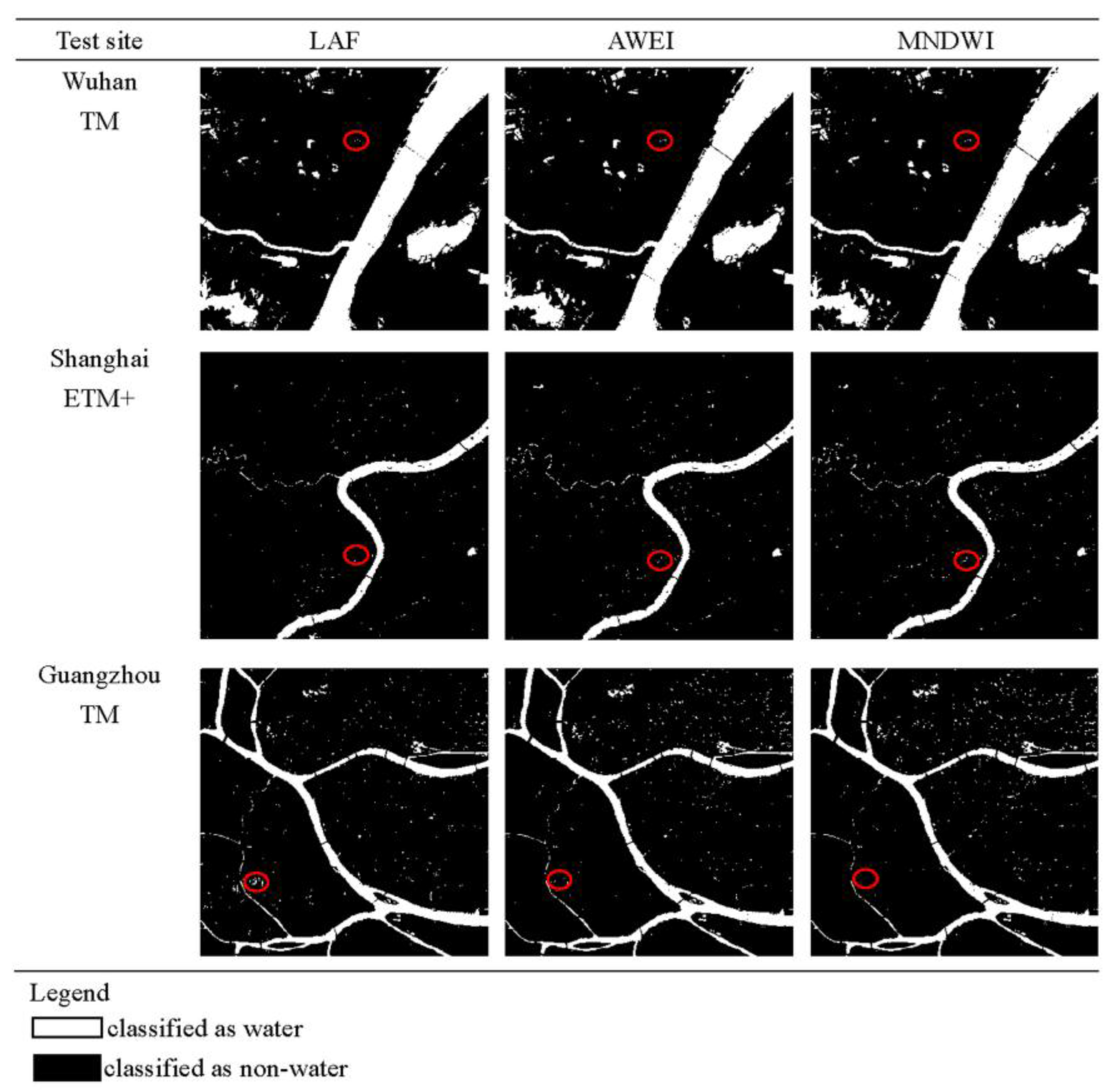
The water extraction results using the three methods of MNDWI, AWEI, and LAF at the three test sites are illustrated in Figure 5. A visual inspection of the figure indicates that LAF results in a better (or at least comparable) accuracy of urban surface water mapping than the AWEI and MNDWI. For the test sites of Wuhan and Shanghai, in particular, the LAF method performs better in suppressing non-water surfaces. Unfortunately, at the test site in Guangzhou, a visual inspection of Figure 5 tells us that the proposed method produces noisy results, as do the other two methods.
Table 3 lists extraction accuracies of urban surface water at the per-pixel level from the three methods at the three test sites. For the overall per-pixel accuracy assessment, 400 testing samples were randomly sampled from the image scene of each test sites. The results show that the KCs of LAF outperform those of MNDWI and AWEI at the Wuhan and Shanghai test sites, whereas LAF does not perform as well as MNDWI and AWEI at the Guangzhou test site. Therefore, from the above observations, we can conclude that LAF achieves a better, or at least comparable, per-pixel extraction accuracy for urban surface water than MNDWI and AWEI.
4.2. Sub-Pixel Accuracy Assessment of LAF in Boundary Mixed Pixels
We also compare extraction accuracies at the sub-pixel level for the three methods. The experiment aims to investigate the performance of LAF in extracting the water from boundary mixed pixels that consist of mixtures of water and non-water components. Table 4 lists extraction errors of the three methods for the boundary mixed pixels at all three test sites. For the sub-pixel accuracy assessment, the testing samples on Wuhan, Shanghai and Guangzhou were randomly chosen along the boundary of Shahu Lake, Huangpu River and Pearl River. The testing samples were mixed by water and concrete pavement, vegetation and soil. The detailed information of three test sites for sub-pixel accuracy assessment is listed in Table 5. The numbers of testing pixels on Wuhan, Shanghai and Guangzhou are 210, 198 and 201, respectively. The accuracies within each water fraction range are the average of AEEs from three test sites.
The results are in agreement for the three methods in that boundary mixed pixels consisting of 0–10% and 90–100% water are correctly classified as non-water and water, respectively. However, the performance of the three methods varies greatly in extracting water having proportions of 10–90% in the boundary mixed pixels. For the 10–90% boundary pixels, AWEI and MNDWI obtain similar extraction accuracies, with AWEI being slightly superior to MNDWI. The accuracy of LAF clearly surpasses that of AWEI and MNDWI, and it reduces extraction errors by at least 5% in the 10–90% proportion of the boundary pixels. Therefore, we conclude that LAF performs significantly better at the sub-pixel level than AWEI and MNDWI.
4.3. Threshold Analysis
Section 3.1 describes that an initial threshold estimation is essential for the parameter tuning of LAF. A good initialization reduces the computational complexity of threshold estimation in LAF, thereby promoting the feasibility of LAF for real-word applications. This experiment therefore explores the stability of the threshold in LAF.
Table 6 lists the parameter settings of the three water extraction methods that produces the best extraction results in experiments 4.1 and 4.2. The standard deviation (Std) is adopted to quantify the variation in threshold parameters of the three methods. The appropriate threshold for MNDWI at the three test sites ranges from 0.35 to 0.515, giving the largest Std in parameter estimation. The appropriate threshold for AWEI varies from 0.086 to 0.2, and the Std is smaller than that of MNDWI but is higher than that of LAF. The comparison shows that the appropriate threshold of LAF shows the smallest variation across the three test sites, with the narrowest range from 1 to 1.08. The appropriate threshold of LAF is close to its initial value of 1, with only slight tuning work required. Therefore, we conclude from the above that the appropriate threshold in LAF has the smallest variation among all the three methods at the three test sites, and the threshold value at 1 is a good and stable initial value for LAF in extracting urban surface water.
5. Discussion
In the above experiments, we implemented LAF to extract urban surface water from Landsat imagery on three metropolises, Wuhan, Shanghai and Guangzhou. The extraction results were evaluated on the aspects of per-pixel accuracy and sub-pixel accuracy and were compared with two state-of-the-art methods, AWEI and MNDWI. All the experimental results demonstrate the superiority of LAF to other two methods.
First, from per-pixel accuracy estimation experiment on three test sites, our LAF shows better performance in differentiating urban surface water from other ground objects (e.g., building roofs, roads, and vegetation), especially in the image scenes of Wuhan and Shanghai. The better per-pixel accuracy results, in our estimation, from two main causes. The first is that the H-L-V linear mixture model could explain reflectance features of land covers in Landsat imagery, while also avoiding nonnegative effects from soil. The second is that multiple selection schemes maximize the divergence of three endmembers of high albedo, low albedo and vegetation, and it guarantees three vertexes of triangular topology in mixing space of all land covers of urban environments.
Second, with regard to sub-pixel accuracy estimation results on three test sites, our LAF behaves better at recognizing water fractions from boundary mixed pixels. The LSU feature of our method guarantees that it is better able to identify water fractions from boundary mixed pixels, using a fraction threshold of low albedo. On the contrary, the AWEI and MNDWI could not avoid the large uncertainty in boundary water pixels originating from the hard-binary classification of water and non-water at the pixel level.
Finally, the threshold analysis explains that the LAF has a relatively more stable threshold than other two methods. For many water extraction methods, the threshold value for binary classification is difficult to estimate because of its data-driven nature [8]. Our LAF has the smallest variations in the threshold on three test sites among all three methods, making the implementation of the method simpler. It is essential to note that the different endmember selection scheme described in [38] would also greatly affect the stability or value of the fraction threshold.
However, our work has several limitations that require further study. The first is that we could not explain theoretical reasons for good behaviors of empirical threshold value as 1. The fraction relations between water and other urban land covers should be carefully analyzed in further experiments to explain the physical meanings of the recommended initial threshold. The second is that we did not carefully investigate the water extraction problem in the presence of cloud and SLC-gaps. Many algorithms including the multi-temporal linear regression algorithm [39] and the GNSPI algorithm [40] have been proposed to detect the thick clouds and fill gap pixels in SLC-OFF Landsat imagery. The combination of the above algorithms with our LAF would be a promising direction to extend the LAF into urban water extraction of any archived Landsat images. The third is that the H-L-V linear mixture model restricts the applications of LAF into other image scenes. It is not difficult to extend the LAF for the purposes of extracting urban wetlands and identifying water fractions from mixed vegetation-water pixels. Unfortunately, the method would not directly apply to other situations, such as open water or coastal wetlands, because the spectral features of their land covers do not satisfy the H-L-V linear mixture model, especially the unavailability of high albedo reflectance such as building roofs and airports. In such cases, other linear mixture models or nonlinear mixture models might be a good addition to the proposed method. The fourth one is that the endmember selection scheme involves too much manual operations and it might restrict the application of LAF to too large an image scene. The automatic or intelligent scheme should be further investigated to satisfy the demands from its complicated image scenes in massive Landsat datasets. The last one is that most recently proposed methods including the enhanced water index (EWI) [39] and dynamic surface water extent (DSWE) [40] have not been considered in comparisons with the LAF. Further performance contrast with modifications of MNDWI and newly-proposed methods on more Landsat images is essential to promote the LAF in real-word applications.
6. Conclusions
The main purpose of this study was to devise a method that improves the sub-pixel water extraction accuracy and has a stable threshold value. Using Urban Landsat images, we presented the LAF method, and then compared its per-pixel and sub-pixel extraction accuracies and threshold stability with those of two state-of-the-art methods, AWEI and MNDWI, at three test sites including Wuhan, Shanghai, and Guangzhou. The results show that LAF achieves a better sub-pixel water extraction accuracy and reduces errors by at least 5% when compared to AWEI and MNDWI, and obtains better, or at least comparable, extraction results at the per-pixel level than the other two methods. Moreover, the method has the smallest variation in appropriate threshold, and the threshold at 1 is a good and stable initialization for parameter tuning in LAF.
Acknowledgments
This work was funded by the National Natural Science Foundation (41671342, 41401389, U1609203) and the Chinese Postdoctoral Science Foundation (2016T90732, 2015M570668). We greatly appreciate the handling editor and the anonymous reviewers for their hard work in reviewing the paper.
Author Contributions
All coauthors made significant contributions to the paper. Weiwei Sun presented the key idea of the LAF method and carried on the contrast experiments. Bo Du designed the comparison experiments between the proposed LAF and the other two methods. Shaolong Xiong helped to design the procedures of experiments in the paper.
Conflicts of Interest
The authors declare no conflict of interest.
References
- Liu, Y.; Bai, X.; Shi, P. Realizing China’s urban dream. Nature 2014, 509, 158–160. [Google Scholar]
- United States Geological Survey (USGS). Facing Tomorrow’s Challenges—U.S. Geological Survey Science in the Decade 2007–2017; U.S. Geological Survey: Reston, VA, USA, 2007.
- Giardino, C.; Bresciani, M.; Villa, P.; Martinelli, A. Application of remote sensing in water resource management: The case study of lake trasimeno, Italy. Water Resour. Manag. 2010, 24, 3885–3899. [Google Scholar] [CrossRef]
- Morss, R.E.; Wilhelmi, O.V.; Downton, M.W.; Gruntfest, E. Flood risk, uncertainty, and scientific information for decision making: Lessons from an interdisciplinary project. Bull. Am. Meteorol. Soc. 2005, 86, 1593–1601. [Google Scholar] [CrossRef]
- Wang, Q.; Lin, J.; Yuan, Y. Salient band selection for hyperspectral image classification via manifold ranking. IEEE Trans. Neural Netw. Learn. Syst. 2016, 27, 1279–1289. [Google Scholar] [CrossRef] [PubMed]
- Zhang, P.; Lu, J.Z.; Feng, L.; Chen, X.L.; Zhang, L.; Xiao, X.W.; Liu, H.G. Hydrodynamic and inundation modeling of China’s largest freshwater lake aided by remote sensing data. Remote Sens. 2015, 7, 4858–4879. [Google Scholar] [CrossRef]
- Wang, Q.; Chen, M.; Li, X. Quantifying and Detecting Collective Motion by Manifold Learning. Proceeding of the AAAI Conference on Artificial Intelligence (AAAI), San Francisco, CA, USA, 4–9 February 2017; pp. 4292–4298. [Google Scholar]
- Ji, L.; Zhang, L.; Wylie, B. Analysis of dynamic thresholds for the normalized difference water index. Photogramm. Eng. Remote Sens. 2009, 75, 1307–1317. [Google Scholar] [CrossRef]
- Feyisa, G.L.; Meilby, H.; Fensholt, R.; Proud, S.R. Automated water extraction index: A new technique for surface water mapping using Landsat imagery. Remote Sens. Environ. 2014, 140, 23–35. [Google Scholar] [CrossRef]
- Lira, J. Segmentation and morphology of open water bodies from multispectral images. Int. J. Remote Sens. 2006, 27, 4015–4038. [Google Scholar] [CrossRef]
- Jiang, H.; Feng, M.; Zhu, Y.; Lu, N.; Huang, J.; Xiao, T. An automated method for extracting rivers and lakes from Landsat imagery. Remote Sens. 2014, 6, 5067–5089. [Google Scholar] [CrossRef]
- Yang, Y.; Liu, Y.; Zhou, M.; Zhang, S.; Zhan, W.; Sun, C.; Duan, Y. Landsat 8 OLI image based terrestrial water extraction from heterogeneous backgrounds using a reflectance homogenization approach. Remote Sens. Environ. 2015, 171, 14–32. [Google Scholar] [CrossRef]
- Jain, S.K.; Singh, R.; Jain, M.; Lohani, A. Delineation of flood-prone areas using remote sensing techniques. Water Resour. Manag. 2005, 19, 333–347. [Google Scholar] [CrossRef]
- Jain, S.K.; Saraf, A.K.; Goswami, A.; Ahmad, T. Flood inundation mapping using noaa avhrr data. Water Resour. Manag. 2006, 20, 949–959. [Google Scholar] [CrossRef]
- McFeeters, S. The use of the normalized difference water index (NDWI) in the delineation of open water features. Int. J. Remote Sens. 1996, 17, 1425–1432. [Google Scholar] [CrossRef]
- Xu, H. Modification of normalised difference water index (NDWI) to enhance open water features in remotely sensed imagery. Int. J. Remote Sens. 2006, 27, 3025–3033. [Google Scholar] [CrossRef]
- Rogers, A.; Kearney, M. Reducing signature variability in unmixing coastal marsh thematic mapper scenes using spectral indices. Int. J. Remote Sens. 2004, 25, 2317–2335. [Google Scholar] [CrossRef]
- Verpoorter, C.; Kutser, T.; Tranvik, L. Automated mapping of water bodies using Landsat multispectral data. Limnol. Oceanogr. Methods 2012, 10, 1037–1050. [Google Scholar] [CrossRef]
- Cracknell, A.P. Review article synergy in remote sensing-What’s in a pixel? Int. J. Remote Sens. 1998, 19, 2025–2047. [Google Scholar] [CrossRef]
- Yuan, Y.; Lin, J.; Wang, Q. Dual-clustering-based hyperspectral band selection by contextual analysis. IEEE Trans. Neural Netw. Learn. Syst. 2016, 54, 1431–1445. [Google Scholar] [CrossRef]
- Sethre, P.R.; Rundquist, B.C.; Todhunter, P.E. Remote detection of prairie pothole ponds in the devils lake basin, north dakota. GISci. Remote Sens. 2005, 42, 277–296. [Google Scholar] [CrossRef]
- Sun, X.; Li, L.; Zhang, B.; Chen, D.; Gao, L. Soft urban water cover extraction using mixed training samples and support vector machines. Int. J. Remote Sens. 2015, 36, 3331–3344. [Google Scholar] [CrossRef]
- Keshava, N.; Mustard, J.F. Spectral unmixing. IEEE Signal Process. Mag. 2002, 19, 44–57. [Google Scholar] [CrossRef]
- Zhou, Y.; Luo, J.; Shen, Z.; Hu, X.; Yang, H. Multiscale water body extraction in urban environments from satellite images. IEEE J. Sel. Top. Appl. Earth Obs. Remote Sens. 2014, 7, 4301–4312. [Google Scholar] [CrossRef]
- Xie, H.; Luo, X.; Xu, X.; Pan, H.; Tong, X. Automated Subpixel Surface Water Mapping from Heterogeneous Urban Environments Using Landsat 8 OLI Imagery. Remote Sens. 2016, 8, 584. [Google Scholar] [CrossRef]
- United States Geological Survey (USGS). Landsat Data Archive; USGS Global Visualization Viewer (GLOVIS): Reston, VA, USA, 2012.
- EXELIS. Exelis Visual Information Solutions; ENVI v5.0; EXELIS: Boulder, CO, USA, 2013. [Google Scholar]
- Lu, D.; Batistella, M.; Moran, E.; Mausel, P. Application of spectral mixture analysis to amazonian land-use and land-cover classification. Int. J. Remote Sens. 2004, 25, 5345–5358. [Google Scholar] [CrossRef]
- Small, C. The Landsat ETM+ spectral mixing space. Remote Sens. Environ. 2004, 93, 1–17. [Google Scholar] [CrossRef]
- Ridd, M.K. Exploring a VIS (vegetation-impervious surface-soil) model for urban ecosystem analysis through remote sensing: Comparative anatomy for cities. Int. J. Remote Sens. 1995, 16, 2165–2185. [Google Scholar] [CrossRef]
- Small, C. Estimation of urban vegetation abundance by spectral mixture analysis. Int. J. Remote Sens. 2001, 22, 1305–1334. [Google Scholar] [CrossRef]
- Wu, C.; Murray, A.T. Estimating impervious surface distribution by spectral mixture analysis. Remote Sens. Environ. 2003, 84, 493–505. [Google Scholar] [CrossRef]
- Small, C. A global analysis of urban reflectance. Int. J. Remote Sens. 2005, 26, 661–681. [Google Scholar] [CrossRef]
- Smith, M.O.; Johnson, P.E.; Adams, J.B. Quantitative determination of mineral types and abundances from reflectance spectra using principal components analysis. J. Geophys. Res. Solid Earth 1985, 90, C797–C804. [Google Scholar] [CrossRef]
- Weng, Q.; Hu, X. Medium spatial resolution satellite imagery for estimating and mapping urban impervious surfaces using lsma and ann. IEEE Trans. Geosci. Remote Sens. 2008, 46, 2397–2406. [Google Scholar] [CrossRef]
- Roberts, D.A.; Gardner, M.; Church, R.; Ustin, S.; Scheer, G.; Green, R.O. Mapping chaparral in the santa monica mountains using multiple endmember spectral mixture models. Remote Sens. Environ. 1998, 65, 267–279. [Google Scholar] [CrossRef]
- Heinz, D.C.; Chang, C.I. Fully constrained least squares linear spectral mixture analysis method for material quantification in hyperspectral imagery. IEEE Trans. Geosci. Remote Sens. 2001, 39, 529–545. [Google Scholar] [CrossRef]
- Nascimento, J.M.P.; Dias, J.M.B. Vertex component analysis: A fast algorithm to unmix hyperspectral data. IEEE Trans. Geosci. Remote Sens. 2005, 43, 898–910. [Google Scholar] [CrossRef]
- Wang, S.; Baig, M.H.A.; Zhang, L.; Jiang, H.; Ji, Y.; Zhao, H.; Tian, J. A simple enhanced water index (EWI) for percent surface water estimation using Landsat data. IEEE J. Sel. Top. Appl. Earth Obs. Remote Sens. 2015, 8, 90–97. [Google Scholar] [CrossRef]
- Jones, J. Efficient wetland surface water detection and monitoring via Landsat: Comparison with in situ data from the everglades depth estimation network. Remote Sens. 2015, 7, 12503–12538. [Google Scholar] [CrossRef]
Figure 1.
The images of Landsat data on three metropolises: (a) Wuhan; (b) Shanghai; and (c) Guangzhou.
Figure 1.
The images of Landsat data on three metropolises: (a) Wuhan; (b) Shanghai; and (c) Guangzhou.

Figure 2.
The overall procedure of the LAF method.
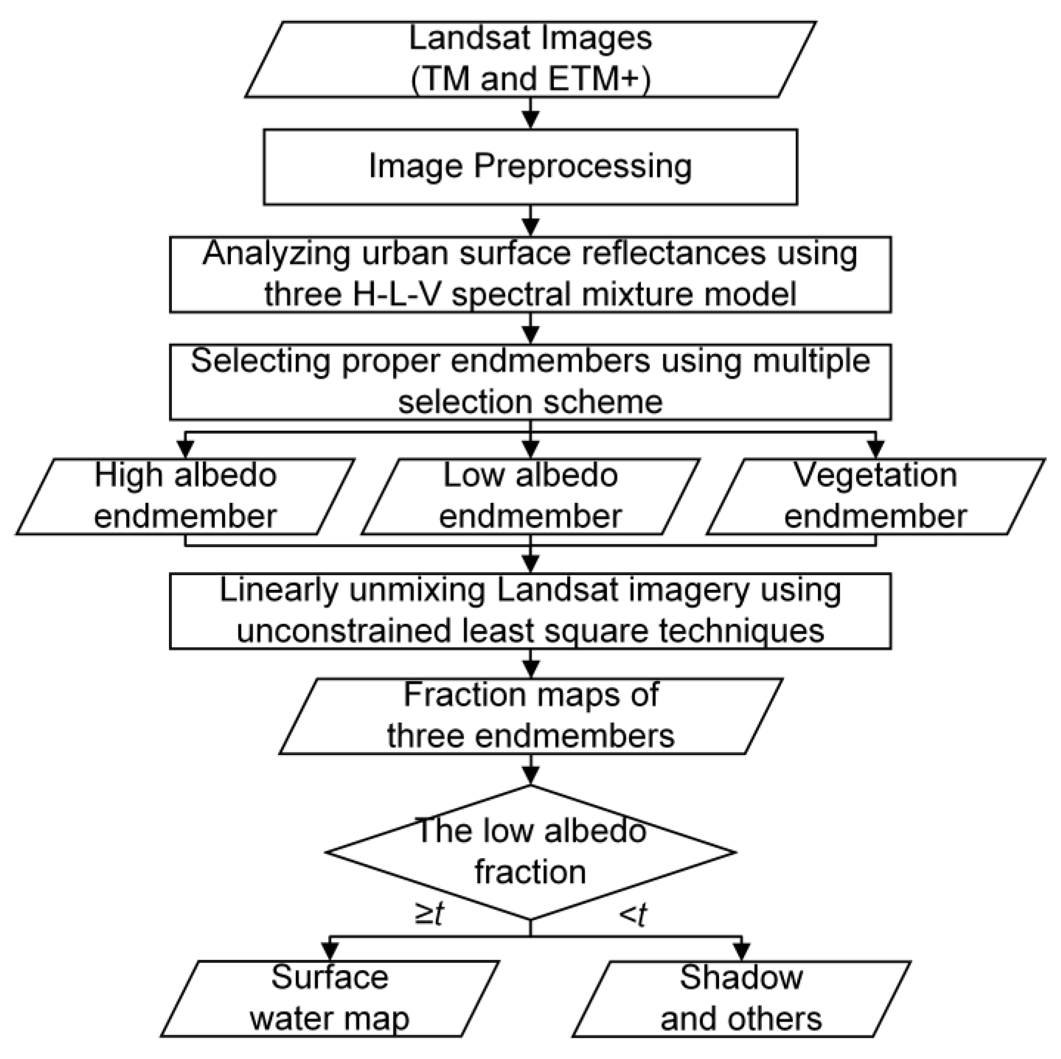
Figure 3.
The triangular topology from scatter plots of the first two PCs. The vertexes correspond to three endmembers: high albedo (e.g., concrete), low albedo (e.g., water), and vegetation (e.g., grass).
Figure 3.
The triangular topology from scatter plots of the first two PCs. The vertexes correspond to three endmembers: high albedo (e.g., concrete), low albedo (e.g., water), and vegetation (e.g., grass).
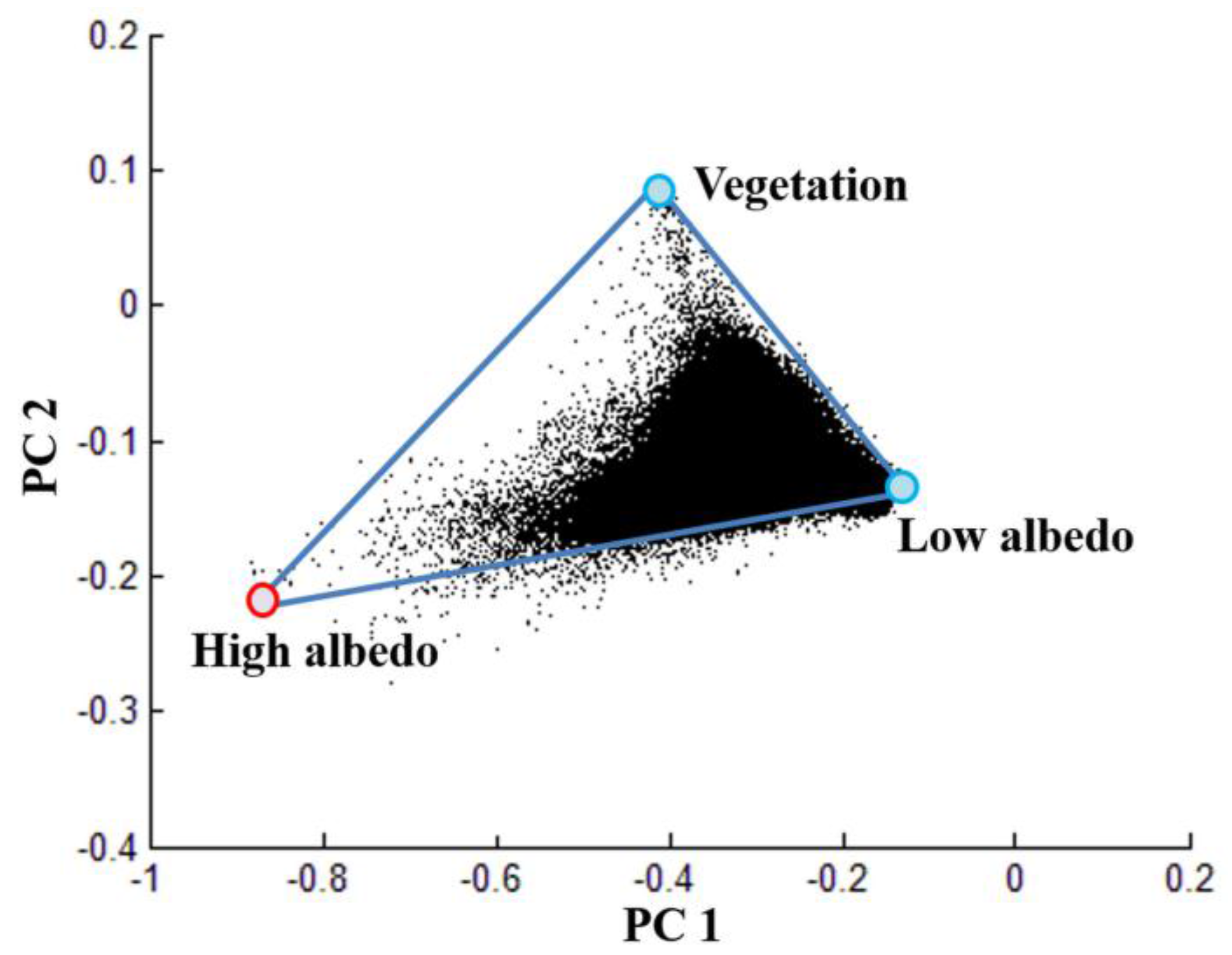
Figure 4.
The category of true water proportions in testing boundary pixels in Shahu lake, Wuhan.

Figure 5.
Comparison of water extraction results from all three methods on three test sites.

Table 1.
Description of Landsat images and their corresponding reference data.
| Test Site | Acquisition Date | Sensors | Path | Row | Source | |
|---|---|---|---|---|---|---|
| Wuhan | Landsat data | 13 September 2000 | TM | 123 | 39 | USGS |
| Reference data | 21 September 2000 | Google Earth ©Digital globe | ||||
| Shanghai | Landsat data | 27 November 2002 | ETM+ | 118 | 38 | USGS |
| Reference data | 28 December 2002 | Google Earth ©Digital globe | ||||
| Guangzhou | Landsat data | 2 January 2009 | TM | 122 | 44 | USGS |
| Reference data | 16 November 2008 | Google Earth ©Digital globe | ||||
Table 2.
The operations of multiple selection schemes in three endmembers.
| Endmembers | Difficulty Level | Key Words in Operation | Candidate Sources |
|---|---|---|---|
| Low albedo | Easy | minimum brightness | deep dark water |
| Vegetation | Easy | maximal normalized difference vegetation index | grass and pasture |
| High albedo | Difficulty | nearest to the high albedo vertex in the triangular topology | building roofs, airport runway and highway intersections |
Table 3.
List of extraction accuracies at the per-pixel level for the three methods at three test sites.
Table 3.
List of extraction accuracies at the per-pixel level for the three methods at three test sites.
| Water Extraction Methods | Kappa Coefficient (KC) | ||
|---|---|---|---|
| Wuhan | Shanghai | Guangzhou | |
| LAF | 0.97 | 0.93 | 0.91 |
| AWEI | 0.95 | 0.92 | 0.93 |
| MNDWI | 0.96 | 0.92 | 0.92 |
Table 4.
List of extraction errors at the sub-pixel level for the three methods with boundary mixed pixels of all three test sites.
Table 4.
List of extraction errors at the sub-pixel level for the three methods with boundary mixed pixels of all three test sites.
| Water Extraction Methods | Extraction Errors of % Water in the Boundary Mixed Pixels | |||||
|---|---|---|---|---|---|---|
| 0–10% | 10–30% | 30–50% | 50–70% | 70–90% | 90–100% | |
| LAF | 0.04 | 0.22 | 0.43 | 0.41 | 0.23 | 0.03 |
| AWEI | 0.04 | 0.30 | 0.49 | 0.47 | 0.34 | 0.03 |
| MNDWI | 0.04 | 0.33 | 0.48 | 0.49 | 0.37 | 0.03 |
Table 5.
The detailed information of three test sites for sub-pixel accuracy assessment.
| City | Name of Water Bodies | Center Point Coordinate (UTM) | Area (km) | Characteristics of Water Bodies | Topography | Climate |
|---|---|---|---|---|---|---|
| Wuhan | Shahu lake | 30°34′04.30′′N, 114°19′41.76′′E | 3.04 | Clear lake | flat | Subtropical wet |
| Shanghai | Huangpu river | 31°14′33.18′′N, 121°29′21.00″E | 6.79 | Turbid river | flat | Subtropical wet |
| Guangzhou | Zhujiang river | 23°06′19.23′′N, 113°14′17.30′′E | 13.69 | Turbid river | flat | Subtropical wet |
Table 6.
Stability analysis for the thresholds of all three water extraction methods.
| Water Extraction Methods | Test Site | Threshold Variability | ||
|---|---|---|---|---|
| Wuhan TM | Shanghai ETM+ | Guangzhou TM | Std | |
| LAF | 1.000 | 1.080 | 1.000 | 0.046 |
| AWEI | 0.086 | 0.200 | 0.156 | 0.057 |
| MNDWI | 0.350 | 0.515 | 0.470 | 0.085 |
© 2017 by the authors. Licensee MDPI, Basel, Switzerland. This article is an open access article distributed under the terms and conditions of the Creative Commons Attribution (CC BY) license (http://creativecommons.org/licenses/by/4.0/).
Share and Cite
MDPI and ACS Style
Sun, W.; Du, B.; Xiong, S. Quantifying Sub-Pixel Surface Water Coverage in Urban Environments Using Low-Albedo Fraction from Landsat Imagery. Remote Sens. 2017, 9, 428. https://doi.org/10.3390/rs9050428
AMA Style
Sun W, Du B, Xiong S. Quantifying Sub-Pixel Surface Water Coverage in Urban Environments Using Low-Albedo Fraction from Landsat Imagery. Remote Sensing. 2017; 9(5):428. https://doi.org/10.3390/rs9050428
Chicago/Turabian StyleSun, Weiwei, Bo Du, and Shaolong Xiong. 2017. "Quantifying Sub-Pixel Surface Water Coverage in Urban Environments Using Low-Albedo Fraction from Landsat Imagery" Remote Sensing 9, no. 5: 428. https://doi.org/10.3390/rs9050428
Note that from the first issue of 2016, this journal uses article numbers instead of page numbers. See further details here.