
Unsupervised Change Detection for Multispectral Remote Sensing Images Using Random Walks

1
The State Key Laboratory of Virtual Reality Technology and Systems, Beihang University, Beijing 100191, China
2
Shijiazhuang Flying College of the PLA Air Force, Shijiazhuang 050073, China
*
Author to whom correspondence should be addressed.
†
These authors contributed equally to this work.
Remote Sens. 2017, 9(5), 438; https://doi.org/10.3390/rs9050438
Submission received: 14 February 2017
/
Revised: 18 April 2017
/
Accepted: 21 April 2017
/
Published: 4 May 2017
Abstract
:In this paper, the change detection of Multi-Spectral (MS) remote sensing images is treated as an image segmentation issue. An unsupervised method integrating histogram-based thresholding and image segmentation techniques is proposed. In order to overcome the poor performance of thresholding techniques for strongly overlapped change/non-change signals, a Gaussian Mixture Model (GMM) with three components, including non-change, non-labeling and change, is adopted to model the statistical characteristics of the different images between two multi-temporal MS images. The non-labeling represents the pixels that are difficult to be classified. A random walk based segmentation method is applied to solve this problem, in which the different images are modeled as graphs and the classification results of GMM are imported as the labeling seeds. The experimental results of three remote sensing image pairs acquired by different sensors suggest a superiority of the proposed approach comparing with the existing unsupervised change detection methods.
1. Introduction
In remote sensing, change detection is to identify the difference between two images of the same scene acquired at different times, which is a critical technique in many remote sensing applications, such as land use change monitoring [1], disaster damage assessment [2,3], urban expansion study [4] and map updating [5], etc. Many factors can affect accuracy of the detection results. Identifying task dependent changes between two images is still a challenging task. Numerous techniques have been proposed. Most of them can be grouped into two categories: supervised and unsupervised approaches.
In supervised approaches, change detection is considered as a binary classification problem using bi-temporal images. In which spatial or/and spectral features are extracted from two images (or difference images). Then, classifiers such as Support Vector Machines (SVM) [6], decision trees [7] and Neural Networks [8,9] are employed to perform the classification. To guarantee a better result, a large number of training samples with human labeled ground truth need to be fed into the classifiers after feature extraction. These methods are known as pre-classification change detection methods. Another widely used strategy in supervised approaches is called post-classification change detection or map-to-map change detection. The first step of these methods involves generation of land cover maps from images of different times. Then, the changes can be easily identified between them. The maps can be produced independently. Thus, pre-processing such as radiometric normalization may not be necessary, and cross-sensors change detection also may not be a difficult issue. However, the major limitation is obvious in which post-classification depends on the quality of land cover maps, which is very difficult to be produced. Therefore, a variety of studies [10,11] have been proposed to improve detection accuracy. The advantage of supervised approaches is that a complete description of transitions and the “from-to” information between two acquisitions can be obtained, and the accuracy of detection results are usually higher than other methods. In spite of success, the demand of large volume training data is very difficult to be satisfied, which limits its application.
Compared with supervised methods, unsupervised methods do not aim to provide the “from-to” information of the changes, but the change/non-change map. Furthermore, they do not need any human labeling process to produce ground truth, which is favored in many practical applications. In this paper, we focus attention on unsupervised change detection in multi-spectral images.
The unsupervised change detection methods are typically applied on the difference images of multi-temporal remote sensing images that can be derived by different ways, including subtraction, ratio, and image transformations (e.g., principle component analysis (PCA), change vector analysis (CVA)) [12,13,14,15,16,17]. The purpose of detection is to label all pixels in the difference images as change or non-change. The thresholding techniques are widely adopted to determine the critical boundary between change and non-change [18,19], such as the minimum error thresholding proposed by Kittler and Illingrowth [20] and the EM (Expectation-Maximization) based method proposed by Bruzzone and Prieto [21]. These methods provide a fast and simple way to generate the change map, and work well in general. However, when change and non-change classes are strongly overlapped in feature space, or when their statistical distribution cannot be modeled accurately, the thresholding techniques can not provide satisfactory results. To tackle this problem, some researchers proposed improved approaches. In [22], Markov Random Field (MRF) is applied to construct a fusion framework of assembling different thresholding algorithms to obtain more robust results. Bovolo et al. [23] proposed a two-phase detection method, in which the point set derived by a selective Bayesian thresholding is treated as a pseudo-training set of a binary semi-supervised SVM classifier to generate change map. Bazi et al. [24] applied an active contour algorithm to the pyramid of difference images to segment them into two parts, which are labeled with change or non-change. In Bazi’s method, Kittler’s thresholding method [20] is used to generate the initial contour. In these methods, thresholding techniques still play an important role, which suggests that the intensity of difference signal is a necessary feature for identification of change and non-change. To solve the overlapped distribution of change and non-change signals, other features such as spatial structure information should be considered.
In this paper, an unsupervised change detection method using random walks is proposed. Random walk is a mathematical formalization of a trajectory that consists of taking successive random steps, which is applied here to determine the boundaries of change and non-change. An image is usually modeled as a connected graph consisting of vertices and edges. The probabilities that random walkers starting at each vertex will first arrive at predefined vertices are the critical part that need to be computed. In [25], Grady proposed an image segmentation method using random walks and presented an analytical and quick algorithm to determine the probabilities. The experimental results demonstrate the superiority of Grady’s method in terms of locating weak boundaries and noise tolerance. However, to perform an unsupervised change detection, the predefined vertices (i.e., pre-labeled pixels) should be identified automatically. The thresholding technique is a reasonable choice for this task. In this paper, we extend Bruzzone’s method [21] and propose an adaptive PCA strategy to enhance the change signals in the difference images. PCA transform is applied to the difference images obtained by pixel-wise subtracting band by band. Each PCA component is considered as a mixture of three kinds of signals: change, non-labeling and non-change, and modeled by a Gaussian Mixture Model (GMM). The EM algorithm is adopted to estimate parameters of GMM for each selected component. Then, the pre-labeled map of each selected component is generated using Bayes rule. Random walks are applied to determined the classes of non-labeling signals. Finally, the change map is obtained by fusing the component change maps.
This paper is organized as follows. A brief review of the random walks algorithm on graphs is given in Section 2. Section 3 describes the proposed unsupervised change detection method. Section 4 provides experimental results of the proposed approach and comparisons with four commonly used methods, including the EM based thresholding method [21], the MRF based method [21], Celik’s method [26] and Bazi’s method [24]. Finally, conclusions are given in Section 4.
2. Random Walks on Graph
Random walk is one of the first stochastic processes studied in probability and continues playing an important role in many applications. When it is applied to the labeling task of an image, the image is usually modeled as a finite connected weighted graph. Therefore, we focus on the random walks on graph.
A graph [27] is usually modeled as a pair of sets such that . The elements are the vertices of the graph G. The elements are the edges of the graph G. An edge denote the edge or connection between two vertices . For a two-dimensional image, each pixel can be treated as a vertex, and the edges can be established with the four-neighbor or eight-neighbor relationship of pixels. The weight of edge is usually used to denote the intensity or color changes in the graph-based images segmentation method [25,28]. In these works, is defined as the typical Gaussian weighting function given by
where and indicate the intensity or color vector of ith and jth pixel, respectively. The degree of vertex is sum of the weights of all edges incident on , .
Suppose there are K labels , and the problem of random walk labeling is to identify the probability that the walker starting at the vertex reaches a vertex pre-labeled by first before the vertex pre-labeled by other labels. For a general graph, this is not a facile task. Fortunately, Doyle and Snell [29] established the connection between the concepts of resistor and electric potential in electric networks and corresponding descriptive quantities of random walks on the graph. If the electric potential at the vertices pre-labeled by are fixed to unity and other pre-labeled are set to zero, the electric potential on the vertex equals probability . The probability problem is converted to finding a harmonic function given its boundary values, i.e., the Dirichlet problem.
A harmonic function is a function that satisfies the Laplace equation
The solution of Dirichlet problem is a harmonic function defined in the region , which minimizes the Dirichlet integral
Considering the application on graph, Grady and Schwartz [30] presents a combinatorial formulation of Dirichlet integral
where L is the combinatorial Laplacian matrix defined as
If all the vertices in the graph G are ordered such that the pre-labeled vertices are first and the non-labeling vertices are second. Equation (4) can be decomposed as
Equation (6) is a system of linear equations with unknown. Because L is a positive semi-defined matrix, the only critical points of will be minima. The critical point yields
represents the potentials or the probabilities of pre-labeled vertices. Considering the probabilities of pre-labeled vertices, it is obvious that if a vertex is pre-labeled by , the probability is one; otherwise, it is zero. Let and indicate the potentials (probabilities) of pre-labeled and non-labeling for . can be obtained by solving Equation (8):
The label assigned to a vertex is determined as
It should be noted that the potential of each pixel for all possible labels should satisfy the constraint as follows:
3. Proposed Unsupervised Change Detection
The proposed technique attempts to extract a reliable subset of change and non-change pixels as the pre-labeled sets, and then obtains the change map using the labeling algorithm based on random walks. It consists of three main parts: (i) enhancement of the change information using an adaptive PCA approach; (ii) extraction of pre-labeled sets based on Bayes rule; (iii) generation of change map using the random walk algorithm.
3.1. Enhancement of the Difference Image Using Adaptive PCA
PCA has been used in change detection for many years and has became one of the most popular techniques for its simplicity and capability of enhancing change information [31]. There are two ways to apply PCA for change detection: (1) put two or more images acquired on the same area at different times into a single file and then perform PCA and analyse the minor component images for change information; and (2) perform PCA separately and then analyse the difference images between the multi-temporal PC images [32]. Identifying the best component to represent the change and selecting appropriate thresholds are challenging tasks, especially when different kinds of changes exist. In this work, an adaptive PCA approach is proposed.
Let and denote two multi-spectral images of the same scene acquired at different times. Each pixel in a multi-spectral image is represented as a spectral vector, , where i is index of a pixel. b represents the bth band of image and B is the number of spectral bands. It is often assumed that and have been co-registered and calibrated to reduce the differences in spatial, lighting, and atmospheric conditions between them. Following the CVA method [33], change vector of each pixel is obtained by subtracting operation . PCA transform is applied to all change vectors. The transformed component vectors can be represented as , in which the components are sorted in the order of decreasing eigenvalues. The components with absolute values are used in the change detection procedure. In the following sections, denotes the absolute value of the ith pixel in the bth component.
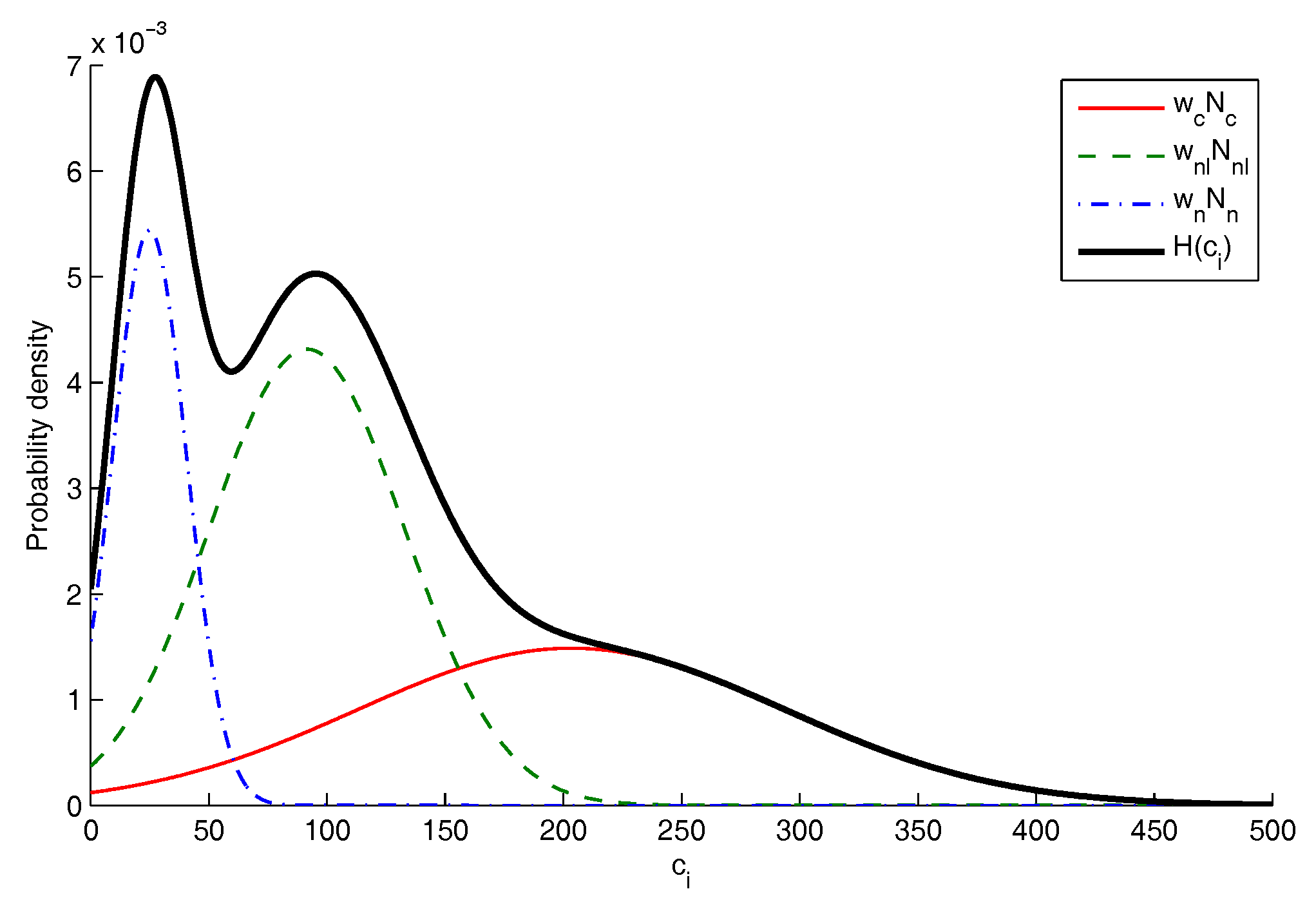
We assume that all pixels in each component can be classified into three groups: change, non-change and non-labeling. Pixels having lower or higher change amplitudes are grouped to non-change or change. Pixels that are difficult to be labeled as change or non-change belong to the non-labeling class. The statistical characters of each category are modeled by a Gaussian distribution . Then, the histogram of a PCA component is represented by a GMM, as shown in Equation (11) and Figure 2:
, and are the weights of the distribution models of change, non-labeling and non-change, and should satisfy the following two constraints:
Because the absolute values of difference images are used here, the means of these three signals should satisfy the following InEquation (14):
All parameters w, and in Equation (11) can be estimated using the EM algorithm.
The enhancing effect of PCA lies in making the change signal easy to be separated from non-change and non-labeling. The separability between two classes can be measured by the Mahalanobis distance of two class centers:
Considering the relationship among these three signals, the distances between change and non-labeling, or non-change is preferred to be larger. On the contrary, the distance between non-labeling and non-change should be smaller. Therefore, an index F is defined as Equation (16) to measure the distinctness of change signals
Based on this measurement, the component selection algorithm is described as follows:
- Step 1:
- Initialize the selection threshold t, .
- Step 2:
- Normalize as Equation (17) and sort in decreasing order:
- Step 3:
- If , then the corresponding component is the unique selected component.
- Step 4:
- Otherwise, repeatedly abandon the component with , until the sum of the rest is less than or equals to t. Then, the remaining components are selected for change detection.
The threshold t is recommended to be not less than . When t is set to 1, it means all PCA components are selected.
3.2. Identification of Pre-Labeled Set Based on Bayes Rule
In Section 3.1, the histogram of a component is modeled with GMM. Equation (11) can be rewritten in its probability form:
where , , and indicate the labels of the three signal classes. It is reasonable to use the Bayes rule to label each pixel in the selected component, as shown in Equation (19). The pre-labeled set is generated by extracting the pixels whose labels are or :
However, the noise in the selected components still has an impact on labeling accuracy. To alleviate this problem, a method is proposed based on Gaussian stack. In the Gaussian stack, the original component is treated as the bottom level . The nth level of the stack is represented as Equation (20):
where indicates a rotationally symmetric Gaussian filter, w is the filter size, and is the standard deviation. The final pre-labeled set is obtained by merging the labeling results of and as follows:
It should be noted that the arguments of Gaussian filter w, , and the number l of stack level are all used to control the Gaussian stack. To simplify the parameter setting, only l was treated as a variant, w and are fixed at 5 and 3, respectively.
3.3. Generation of Change Map Based on Random Walks
For each selected component, the pre-labeled sets of non-change and change are treated as the seeds of the random walks algorithm introduced in Section 2. Each non-labeling pixel is assigned a certain label or . The labeling algorithm [25] can be summarized as follows:
- Step 1:
- Initialize the selected component and the pre-labeled map and .
- Step 2:
- Construct matrix L using Equation (1).
- Step 3:
- Solve Equation (8) to obtain the potentials for non-change label. The potential for change label can be derived by for computational efficiency.
- Step 4:
- Assign a label to each non-labeling pixel according to Equation (9).
Considering the information of different change types is enhanced and represented in different PCA components, the change map is obtained by summing the labeled results of all selected components as Equation (23)
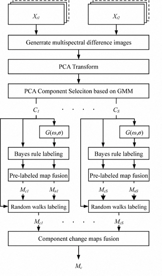
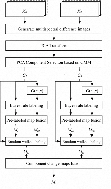
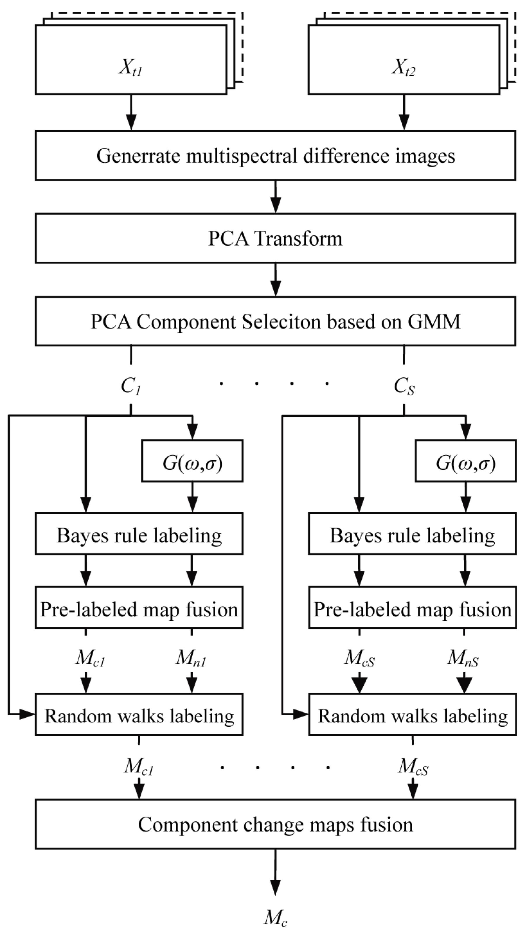
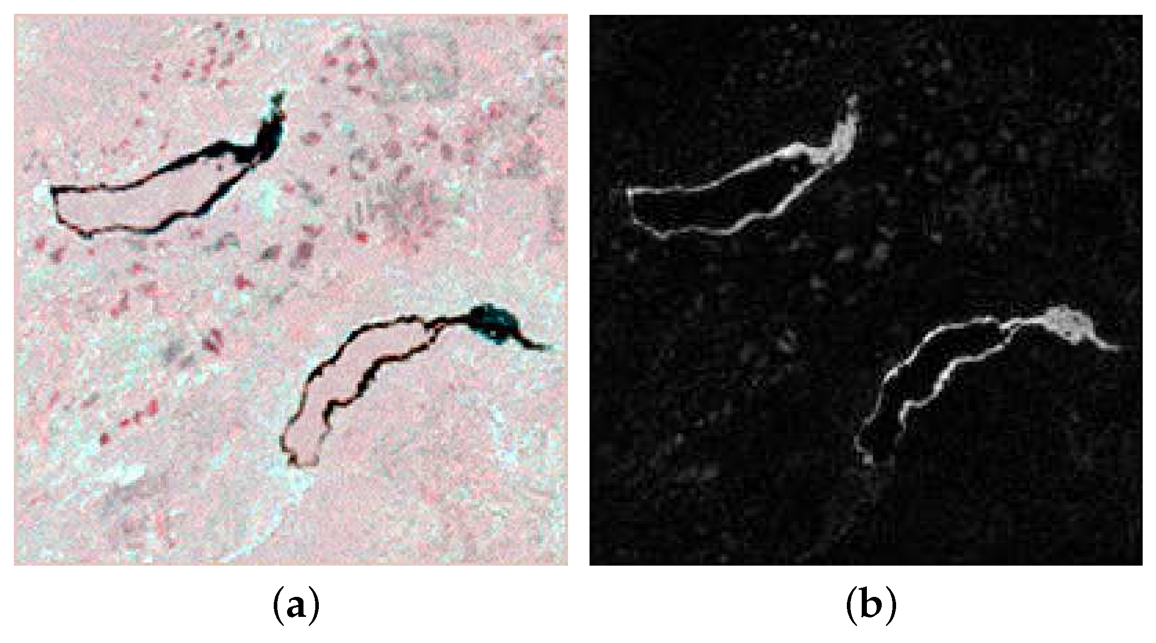
The whole procedure of the proposed unsupervised change detection approach is illustrated in Figure 3. Figure 4 shows an example of the overall process of our method from the difference images to the generation of change map. The proposed adaptive PCA-based method is applied to the difference image (Figure 4a) to extract the representative principle components (PCs) (Figure 4b) containing the change information. Then, the selected components are labeled with change (red), non-change (green) and non-labeling (black) based on the Bayes rule, as shown in Figure 4c. The pre-labeled map and the selected components are fed to the random walk algorithm. Each non-labeling pixel is assigned to a label that has the maximum potential (probability). Finally, the change map as shown in Figure 4d can be obtained.
4. Experiments
In order to assess effectiveness of the proposed unsupervised change detection method, three multi-temporal image pairs are selected as test data sets as shown in Figure 5, Figure 6 and Figure 7, which were acquired by different sensors and contain various land cover changes. The proposed method is compared with four widely used change detection methods on the test data sets.
4.1. Data Sets
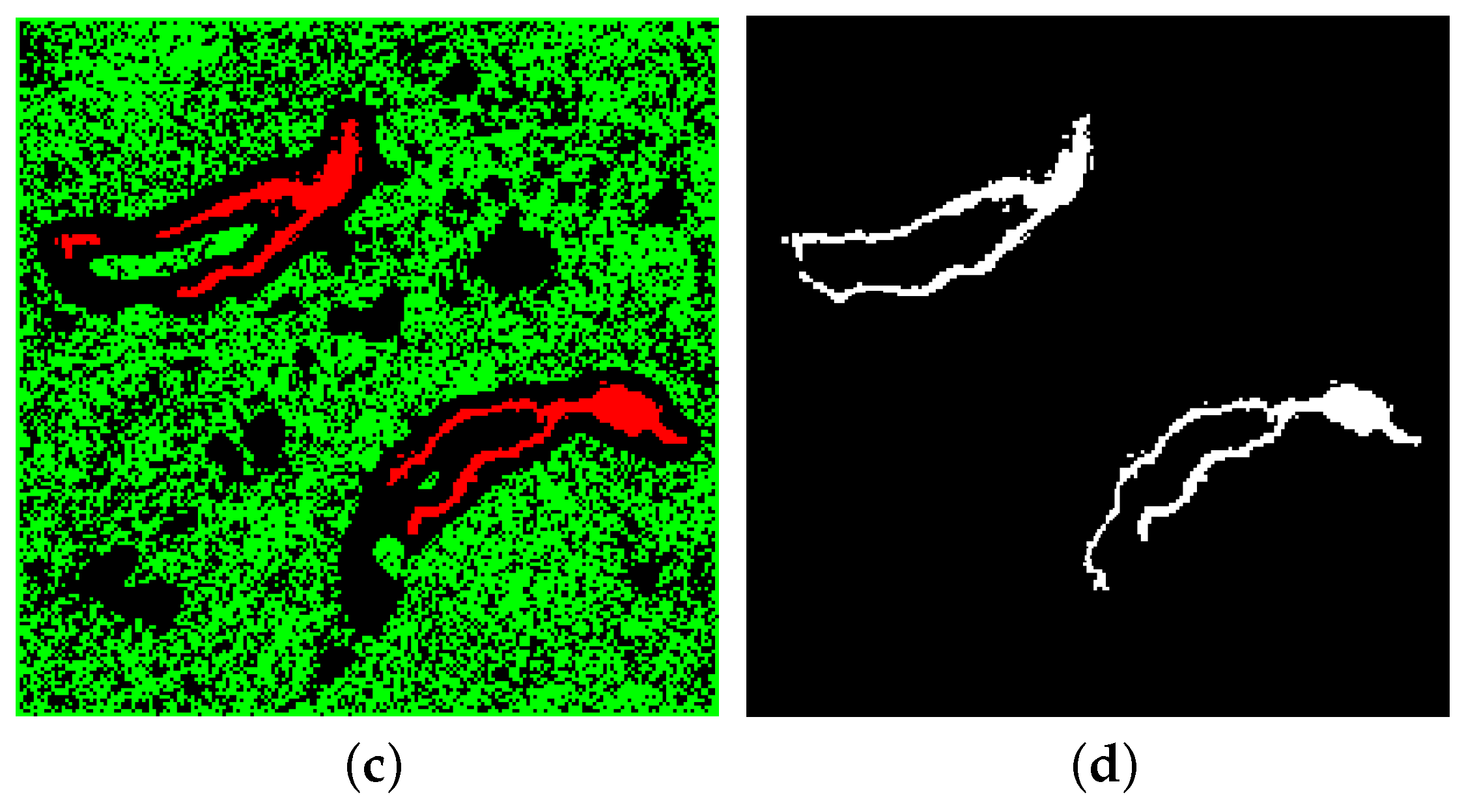
The first data set as shown in Figure 5a,b are two -pixel subsets of three-band images retrieved from [35]. These images are acquired by a Landsat 5 Thematic Mapper (TM), respectively, on 4 October 1996 and 2 June 2009, over the Hobet mine in Boone County, West Virginia. The 15-year mining operation destroyed the vegetation and caused great changes to the land cover.
The second data set as shown in Figure 6a,b refer to -pixel subsets of the ASTER (Advanced Spaceborne Thermal Emission and Reflection Radiometer) VNIR (visible and near-infrared, three bands) data acquired, respectively, on 6 May 2005 and 19 July 2005, over the Mountain Hillers, Utah. The main difference between them is that there is no snow cover region in Figure 6a because of seasonal change.
The third data set, as shown in Figure 7a,b, are two -pixel subsets of the very high resolution multi-spectral (visible and near-infrared, four bands) images generated using pan-sharpening techniques [36] based on the data acquired by QuickBird Satellite on 11 October 2008 and 13 September 2009 over the Shijingshan District, Beijing, China. There are many land cover changes caused by human activities.
4.2. Parameter Setting
In the proposed method, there are three parameters that need to be specified, including the component selection threshold t, the number l of Gaussian stack and the Gaussian weighting parameter in Equation (1). t determines the number of selected PCA components. As mentioned in Section 3.1, it is recommended in the range of . Generally, the level number of Gaussian stack l is a trade-off between the minimum isolate change region and the strength of noise. It will result in no pre-labeled pixels existing in the small change region if l is set to a higher value. Considering that data at a high spatial resolution contains more noise factors than that at low spatial resolution, such as the view angle and the sun angle, and the value of l assigned for the pan-sharpened QuickBird data is higher than that for TM and ASTER data. In this work, we set for ASTER and TM images and for Quickbird images. For the Gaussian weighting parameter , we set as recommended in [26].
4.3. The Effect of the Adaptive PCA Approach
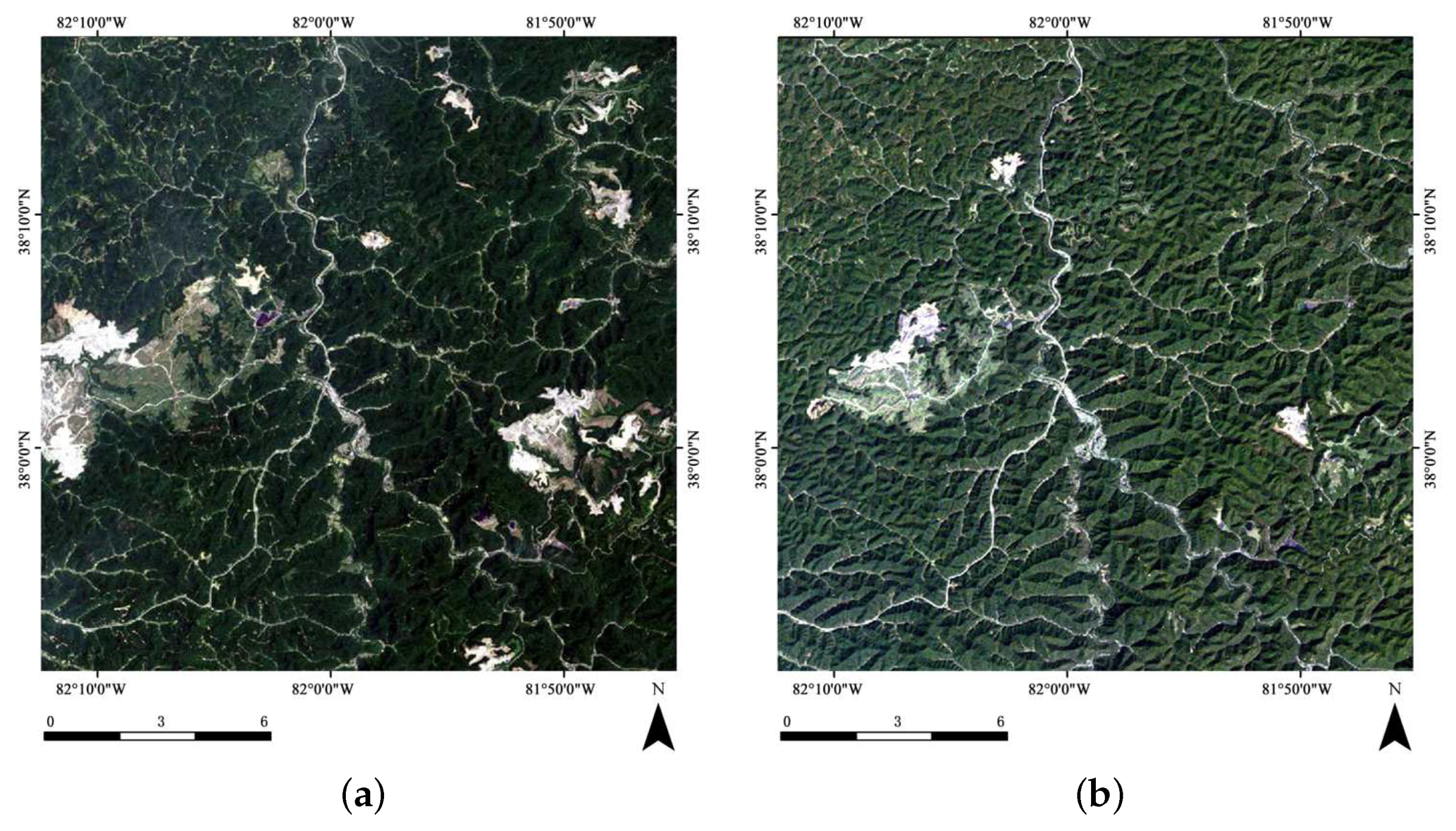
The adaptive PCA approach presented in Section 3.1 is applied on the difference images to extract the components containing enhanced change information. This is the fundamental phase of this method. The threshold t is empirically set to 0.8 for all test data. Figure 9a–d show four PCs of QuickBird difference images and their normalized indices. Intuitively, the components containing more enhanced change signals have a higher values of . Based on this assumption, Figure 9b,c should be selected as a representative component for QuickBird images. From Table 1, it can be seen that the proposed index successfully identify true components. From Figure 9e,f and Table 1, it can also be concluded that the component selected by visual inspection and the proposed index are consistent both in TM and ASTER images.
4.4. Comparisons with Other Change Detection Methods
In order to illustrate the effectiveness of the proposed change detection method (PCA-RW for short), it is compared with four commonly used unsupervised change detection approaches: (1) EM based thresholding method [21]; (2) MRF-based method [21], in which Besag’s iterated conditional modes (ICM) algorithm [38] is used to minimize the MRF energy function initialized by EM algorithm; (3) Block-PCA method (BPCA) [26], in which PCA is applied to non-overlapping block set to detect the change area; (4) and multi-resolution level set method (MLSK) [24], in which the Chan–Vese algorithm [39] is applied on the pyramid of difference images to obtain the change map. These existing methods all depend on some parameters except for the EM based method. In the MRF-based method, tunes the influence of the spatial contextual information during the change detection process. The size h of the image block needs to be set in the BPCA method. In the MLSK method, the regulation parameter controls the tradeoff between the goodness of fit and the length of the profile curve. In this paper, all of these parameters are tuned to achieve the best results for the test data, which are , , . For the proposed method, the level number of Gaussian stack is used.
The performance of these methods are evaluated using the following three standard error measures:
- False-alarm rate ,where is the number of unchanged pixels classified as changed pixels, and is the total number of unchanged pixels.
- Missed-alarm rate ,where is the number of changed pixels classified as unchanged pixels, and is the total number of changed pixels.
- Error rate is the total number of wrongly classified pixels over the total number of pixels,
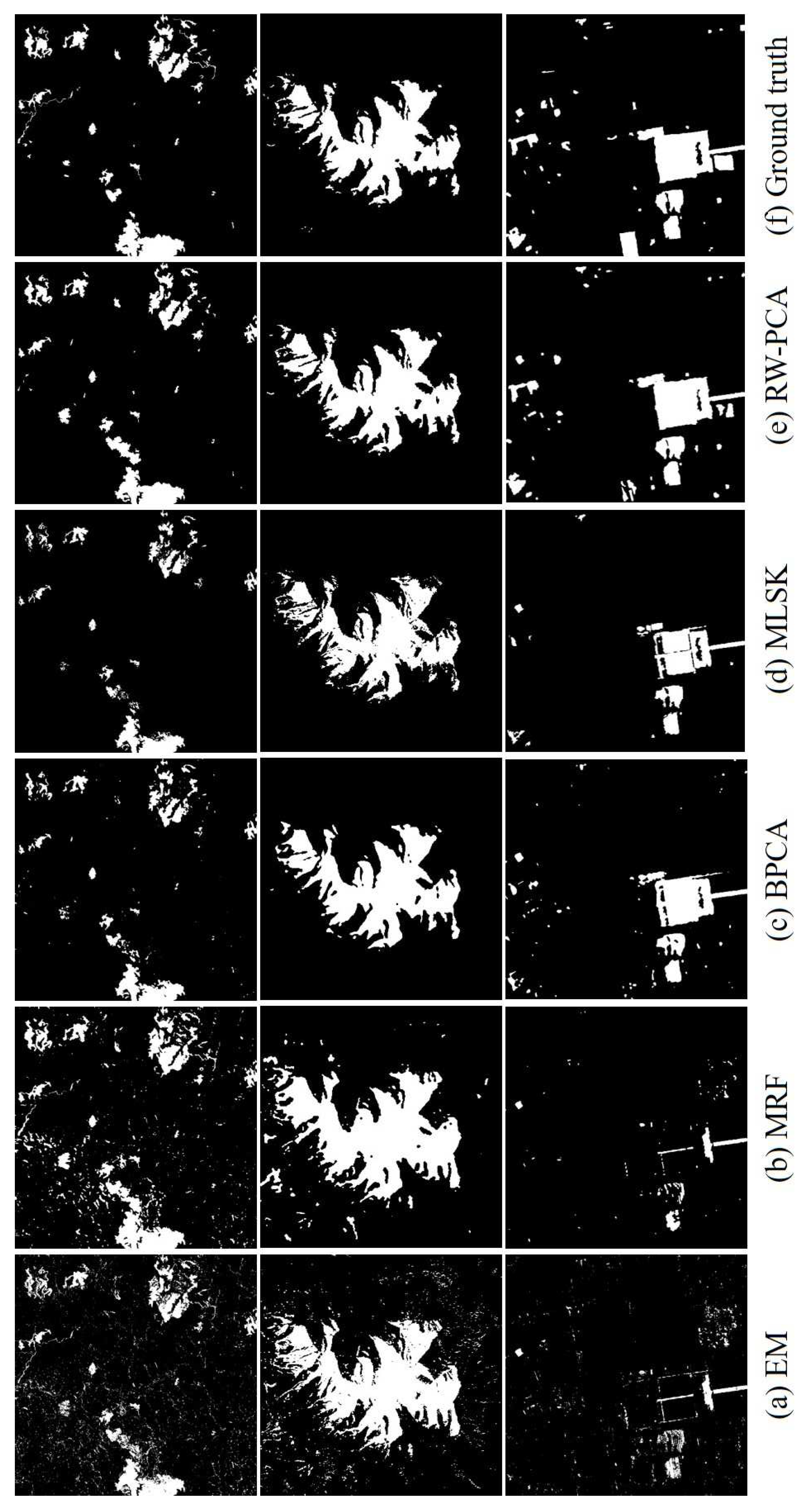
Figure 10 shows change maps obtained by the proposed and four compared methods on the three test image pairs. From Figure 10a, it can be seen that the EM based method produces worst results on all three data sets. There is a lot of noise in TM and ASTER images. Note that a large part of the building is missing in results of Quickbird images. In Figure 10b, the MRF based method also exhibits significant noise in results of TM images. Noise still exists in ASTER images but is reduced to a lower level. A similar part is missing in the change map of Quickbird images. BPCA produces results similar to that of MLSK in the three data sets. However, careful inspection may find that there exist some missing parts on both results of QuickBird images (see the last row of Figure 10c,d). It can be observed from Figure 10e that the proposed method provides results very close to ground truth maps.
Table 2 gives quantitative results on the three data sets. It can be easily seen that the EM method produces results with worst measure indexes. The MRF based method has the best on the TM images. The noise in TM results actually classify more pixels into changed ones, leading to a lower and higher . This is consistent with visual inspection. The BPCA method obtains relatively good results with neither lowest nor highest measure indexes. MLSK shows its efficiency in terms of false-alarm rate with best on all three data sets, which means that almost all pixels classified as changed are correct. To this end, algorithms should have a rigorous criterion to decide which pixels are changed ones, which will have a severe impact on and . This can be observed in Table 2. The proposed method outperforms other methods for overall error rate , which also demonstrates its advantage in reducing the missing alarm. It can be inferred that PCA-RW can make a trade-off between missed-alarm and false alarm rates. Furthermore, it is suitable for detecting multiple types of changes.
5. Conclusions
This paper presents an unsupervised change detection method based on random walks for multi-spectral remote sensing images. Normally, supervised methods obtain better results than unsupervised ones because knowledge about changed and unchanged information are used during training steps. This work can be considered as a special case of a “semi-supervised” method. Firstly, an adaptive PCA approach is proposed to enhance and extract the change information between multi-temporal images. Subsequently, a GMM is applied to obtain three category labels, including changed, unchanged labels and undermined labels. Then, the pre-labeled changed and unchanged mask is fed to a random walk algorithm to obtain the labels of undermined pixels. In this process, the pre-labeled changed and unchanged pixels can be considered as “training samples”. They implicitly contain change and unchanged information. Because no external data is used, the proposed method can still be called “unsupervised” change detection. The method is tested on three image pairs acquired by ASTER, TM and QuickBird and compared with EM, MRF, BPCA and MLSK methods. Results demonstrate that the proposed approach can generate promising change maps. Although there is a smaller sacrifice on , our method can obtain better quantitative indexes in terms of and .
Acknowledgments
The authors would like to thank the anonymous reviewers for their valuable comments and suggestions to improve the quality of this paper. This work is funded by the National Natural Science Foundation of China (No. 61601011) and the National Major Program on High Resolution Earth Observation Systems under Grant 03-Y30B06-9001-13/15-01.
Author Contributions
Qingjie Liu and Lining Liu conceived and designed the experiments. Lining Liu and Qingjie Liu performed the experiments; Qingjie Liu analyzed the data; Yunhong Wang contributed analysis tools; Qingjie Liu and Lining Liu wrote the paper.
Conflicts of Interest
The authors declare no conflict of interest.
Abbreviations
The following abbreviations are used in this manuscript:
| MS | Multi-Spectral |
| SVM | Support Vector Machine PCA: Princpal Component Analysis |
| CVA | Change Vector Analysis |
| MRF | Markov Random Field |
| GMM | Gaussian Mixture Model |
| ASTER | Advanced Spaceborne Thermal Emission and Reflection Radiometer |
| VNIR | Visible and Near-Infrared |
| TM | Thematic Mapper |
| MLSK | multi-resolution level set method |
| BPCA | Block PCA |
| EM | Expectation Maximization |
| ICM | Iterated Conditional Models |
References
- Vittek, M.; Brink, A.; Donnay, F.; Simonetti, D.; Desclée, B. Land cover change monitoring using Landsat MSS/TM satellite image data over West Africa between 1975 and 1990. Remote Sens. 2014, 6, 658–676. [Google Scholar] [CrossRef]
- Krishnan, A.K.; Nissen, E.; Saripalli, S.; Arrowsmith, R.; Corona, A.H. Change detection using airborne LiDAR: Applications to earthquakes. In Experimental Robotics; Springer: Berlin/Heidelberg, Germany, 2013; pp. 733–743. [Google Scholar]
- Byun, Y.; Han, Y.; Chae, T. Image fusion-based change detection for flood extent extraction using bi-temporal very high-resolution satellite images. Remote Sens. 2015, 7, 10347–10363. [Google Scholar] [CrossRef]
- Mertes, C.M.; Schneider, A.; Sulla-Menashe, D.; Tatem, A.; Tan, B. Detecting change in urban areas at continental scales with MODIS data. Remote Sens. Environ. 2015, 158, 331–347. [Google Scholar] [CrossRef]
- Awrangjeb, M. Effective generation and update of a building map database through automatic building change detection from LiDAR point cloud data. Remote Sens. 2015, 7, 14119–14150. [Google Scholar] [CrossRef]
- Volpi, M.; Tuia, D.; Bovolo, F.; Kanevski, M.; Bruzzone, L. Supervised change detection in VHR images using contextual information and support vector machines. Int. J. Appl. Earth Obs. Geoinf. 2013, 20, 77–85. [Google Scholar] [CrossRef]
- Gao, F.; de Colstoun, E.B.; Ma, R.; Weng, Q.; Masek, J.G.; Chen, J.; Pan, Y.; Song, C. Mapping impervious surface expansion using medium-resolution satellite image time series: A case study in the Yangtze River Delta, China. Int. J. Remote Sens. 2012, 33, 7609–7628. [Google Scholar] [CrossRef]
- Wang, Q.; Shi, W.; Atkinson, P.M.; Li, Z. Land cover change detection at subpixel resolution with a Hopfield neural network. IEEE J. Sel. Top. Appl. Earth Obs. Remote Sens. 2015, 8, 1339–1352. [Google Scholar] [CrossRef]
- Lyu, H.; Lu, H.; Mou, L. Learning a transferable change rule from a recurrent neural network for land cover change detection. Remote Sens. 2016, 8, 506. [Google Scholar] [CrossRef]
- El-Kawy, O.A.; Rød, J.; Ismail, H.; Suliman, A. Land use and land cover change detection in the western Nile Delta of Egypt using remote sensing data. Appl. Geogr. 2011, 31, 483–494. [Google Scholar] [CrossRef]
- Sinha, P.; Kumar, L.; Reid, N. Rank-based methods for selection of landscape metrics for land cover pattern change detection. Remote Sens. 2016, 8, 107. [Google Scholar] [CrossRef]
- Singh, A. Review article digital change detection techniques using remotely-sensed data. Int. J. Remote Sens. 1989, 10, 989–1003. [Google Scholar] [CrossRef]
- Melgani, F.; Moser, G.; Serpico, S.B. Unsupervised change-detection methods for remote-sensing images. Opt. Eng. 2002, 41, 3288–3297. [Google Scholar]
- Celik, T.; Ma, K. Unsupervised change detection for satellite images using Dual-Tree complex wavelet transform. IEEE Trans. Geosci. Remote Sens. 2010, 48, 1199–1210. [Google Scholar] [CrossRef]
- Liu, S.; Bruzzone, L.; Bovolo, F.; Du, P. A novel sequential spectral change vector analysis for representing and detecting multiple changes in hyperspectral images. In Proceedings of the 2014 IEEE International Geoscience and Remote Sensing Symposium, Quebec City, QC, Canada, 13–18 July 2014; pp. 4656–4659. [Google Scholar]
- Zhuang, H.; Deng, K.; Fan, H.; Yu, M. Strategies combining spectral angle mapper and change vector analysis to unsupervised change detection in multispectral images. IEEE Geosci. Remote Sens. Lett. 2016, 13, 681–685. [Google Scholar] [CrossRef]
- Chen, Q.; Chen, Y. Multi-feature object-based change detection using self-adaptive weight change vector analysis. Remote Sens. 2016, 8, 549. [Google Scholar] [CrossRef]
- Rosin, P.L. Thresholding for change detection. Comput. Vis. Image Underst. 2002, 86, 79–95. [Google Scholar] [CrossRef]
- Sezgin, M.; Sankur, B. Survey over image thresholding techniques and quantitative performance evaluation. J. Electron. Imaging 2004, 13, 146–165. [Google Scholar]
- Kittler, J.; Illingworth, J. Minimum error thresholding. Pattern Recognit. 1986, 19, 41–47. [Google Scholar] [CrossRef]
- Bruzzone, L.; Prieto, D.F. Automatic analysis of the difference image for unsupervised change detection. IEEE Trans. Geosci. Remote Sens. 2000, 38, 1171–1182. [Google Scholar] [CrossRef]
- Melgani, F.; Bazi, Y. Markovian fusion approach to robust unsupervised change detection in remotely sensed imagery. IEEE Geosci. Remote Sens. Lett. 2006, 3, 457–461. [Google Scholar] [CrossRef]
- Bovolo, F.; Bruzzone, L.; Marconcini, M. A novel approach to unsupervised change detection based on a semisupervised SVM and a similarity measure. IEEE Trans. Geosci. Remote Sens. 2008, 46, 2070–2082. [Google Scholar] [CrossRef]
- Bazi, Y.; Melgani, F.; Al-Sharari, H. Unsupervised change detection in multispectral remotely sensed imagery with level set methods. IEEE Trans. Geosci. Remote Sens. 2010, 48, 3178–3187. [Google Scholar] [CrossRef]
- Grady, L. Random walks for image segmentation. IEEE Trans. Pattern Anal. Mach. Intell. 2006, 28, 1768–1783. [Google Scholar] [CrossRef] [PubMed]
- Celik, T. Unsupervised change detection in satellite images using principal component analysis and k-means clustering. IEEE Geosci. Remote Sens. Lett. 2009, 6, 772–776. [Google Scholar] [CrossRef]
- Diestel, R. Graph Theory, 4th ed.; Graduate Texts in Mathematics; Springer: Berlin/Heidelberg, Germany, 2010; Chapter 1; Volume 173. [Google Scholar]
- Boykov, Y.; Funka-Lea, G. Graph cuts and efficient N-D image segmentation. Int. J. Comput. Vis. 2006, 70, 109–131. [Google Scholar] [CrossRef]
- Doyle, P.G.; Snell, J.L. Random Walks and Electric Networks; The Mathematical Association of America: Washington, DC, USA, 1984. [Google Scholar]
- Grady, L.; Schwartz, E. Anisotropic Interpolation on Graphs: The Combinatorial Dirichlet Problem; Technical Report; Boston University Center for Adaptive Systems and Department of Cognitive and Neural Systems: Boston, MA, USA, 2003. [Google Scholar]
- Deng, J.S.; Wang, K.; Deng, Y.H.; Qi, G.J. PCA-based land-use change detection and analysis using multitemporal and multisensor satellite data. Int. J. Remote Sens. 2008, 29, 4823–4838. [Google Scholar] [CrossRef]
- Lu, D.; Mausel, P.; Brondízio, E.; Moran, E. Change detection techniques. Int. J. Remote Sens. 2004, 25, 2365–2401. [Google Scholar] [CrossRef]
- Malila, W.A. Change Vector Analysis—An Approach for Detecting Forest Changes with Landsat; Institute of Electrical and Electronics Engineers: Piscataway, NJ, USA, 1980; pp. 326–336. [Google Scholar]
- USGS. Southwest U.S. Change Detection Images: Reno and Lake Tahoe, Nevada. Available online: http://geochange.er.usgs.gov/sw/changes/natural/reno-tahoe/cuts.html (accessed on 21 May 2013).
- NASA. Feature Articles: Mountaintop Mining, West Virginia. Available online: http://earthobservatory. nasa.gov/Features/WorldOfChange/hobet.php (accessed on 15 April 2013).
- Liu, L.; Wang, Y.; Wang, Y.; Yu, H. Pan-sharpening using an adaptive linear model. In Proceedings of the International Conference on Pattern Recognition, Istanbul, Turkey, 23–26 August 2010; pp. 4512–4515. [Google Scholar]
- Inamdar, S.; Bovolo, F.; Bruzzone, L.; Chaudhuri, S. Multidimensional probability density function matching for preprocessing of multitemporal remote sensing images. IEEE Trans. Geosci. Remote Sens. 2008, 46, 1243–1252. [Google Scholar] [CrossRef]
- Besag, J. On the statistical analysis of dirty pictures. J. R. Stat. Soc. B 1986, 48, 48–259. [Google Scholar] [CrossRef]
- Chan, T.F.; Vese, L.A. Active contours without edges. IEEE Trans. Image Process. 2001, 10, 266–277. [Google Scholar] [CrossRef] [PubMed]
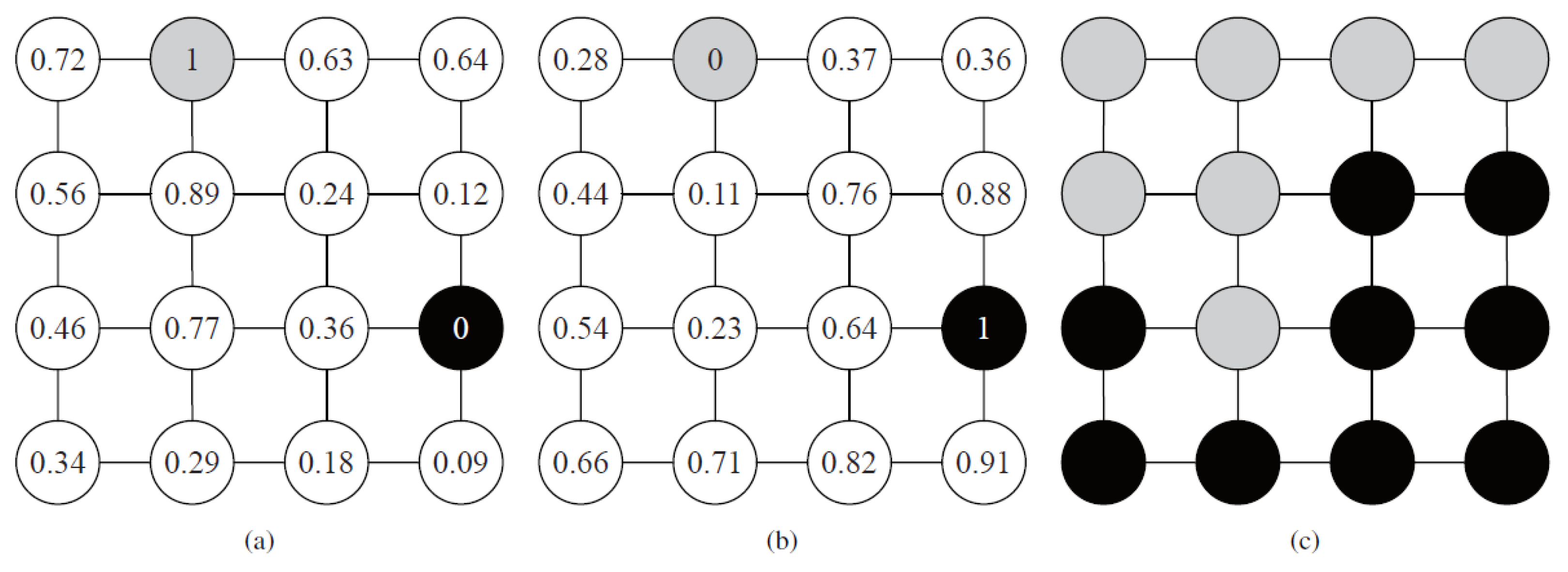
Figure 1.
The labeling procedure using random walks. The vertices pre-labeled with two labels are separately marked with gray and black color. The conditional probability (potential) of each vertex is represented within the circle. (a) probabilities that a random walker starting from each vertices. First reaches the pre-labeled gray vertex; (b) probabilities that a random walker starting from each vertices. First reaches the pre-labeled black vertex; (c) labeled results with the random walk algorithm.

Figure 2.
Histograms of a principal component modeled with three Gaussian distribution: change (c), non-labeling (nl), and non-change (n).
Figure 2.
Histograms of a principal component modeled with three Gaussian distribution: change (c), non-labeling (nl), and non-change (n).

Figure 3.
Flowchart of the proposed unsupervised change detection approach.

Figure 4.
Example of proposed unsupervised change detection. The original multi-temporal images are retrieved from [34]. The first principle component (b) are selected by the algorithm described in Section 3.1, in which . In the pre-labeled map of selected component (c), pixels of change, non-change and non-labeled are represented with red, green and black. The change pixels in (d) are marked with white. (a) false color image obtained by CVA; (b) the component selected by proposed algorithm; (c) pre-labeled map of the selected component; and (d) change map obtained by random walks.


Figure 5.
TM data set. The size of TM images is pixels with 30 m spatial resolution. (a) Hobet mine, TM, 4 October 1996; (b) Hobet mine, TM, 2 June 2009.
Figure 5.
TM data set. The size of TM images is pixels with 30 m spatial resolution. (a) Hobet mine, TM, 4 October 1996; (b) Hobet mine, TM, 2 June 2009.

Figure 6.
ASTER data set. The size of ASTER images is pixels with 15 m spatial resolution. (a) Mountain Hillers, ASTER, 6 May 2005; (b) Mountain Hillers, ASTER, 19 July 2005.
Figure 6.
ASTER data set. The size of ASTER images is pixels with 15 m spatial resolution. (a) Mountain Hillers, ASTER, 6 May 2005; (b) Mountain Hillers, ASTER, 19 July 2005.
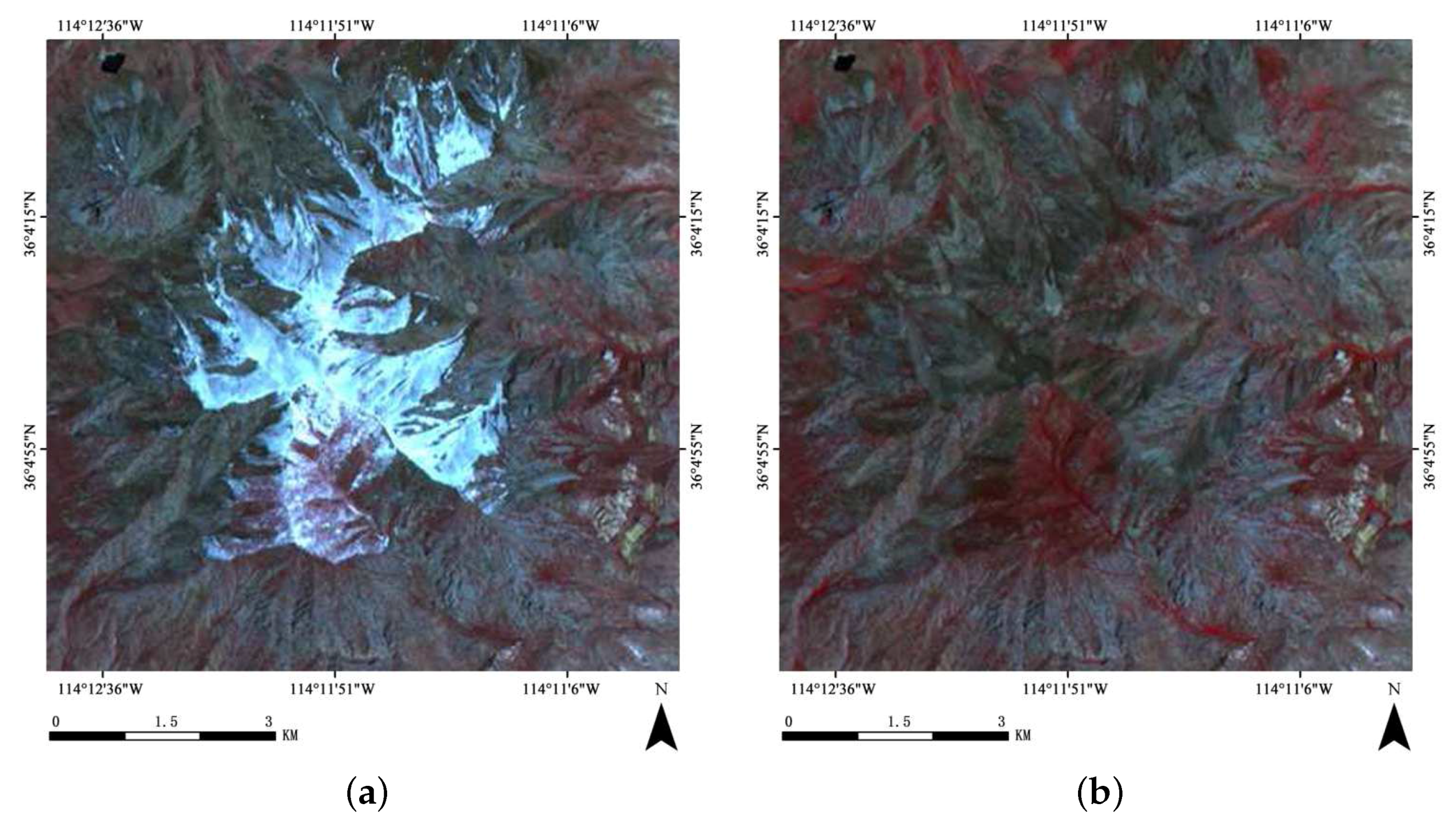
Figure 7.
QuickBird data sets. The size of Quickbird is pixels with 0.6 m spatial resolution. (a) Shijingshan, QuickBird, 11 October 2008; (b) Shijingshan, QuickBird, 13 September 2009.
Figure 7.
QuickBird data sets. The size of Quickbird is pixels with 0.6 m spatial resolution. (a) Shijingshan, QuickBird, 11 October 2008; (b) Shijingshan, QuickBird, 13 September 2009.
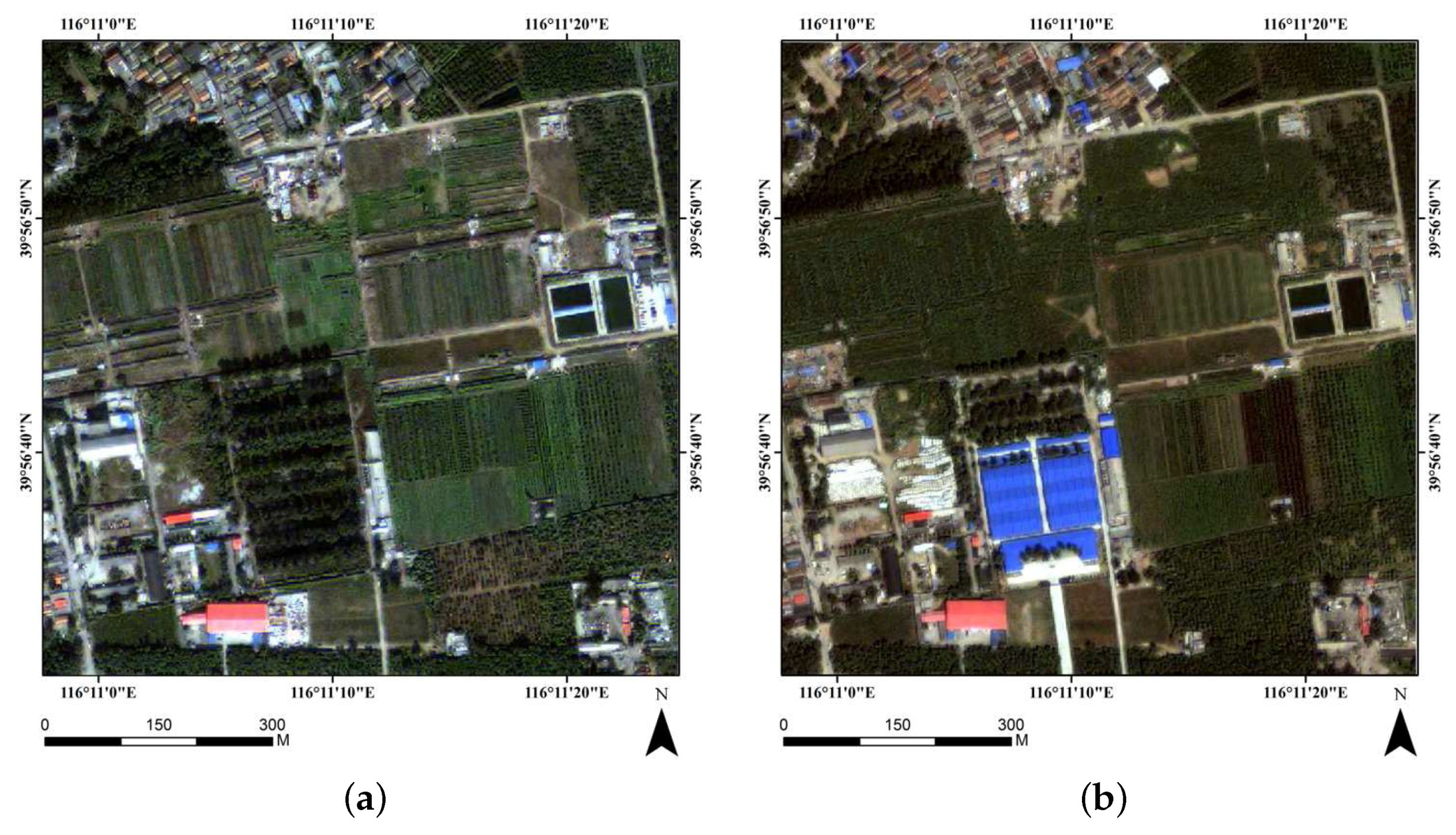
Figure 8.
Manually labeled ground truth for three test data sets. (a) ground truth map of Hobet (TM); (b) ground truth map of Mountain Hiller (ASTER); (c) ground truth map of Shijingshan (QuickBird).
Figure 8.
Manually labeled ground truth for three test data sets. (a) ground truth map of Hobet (TM); (b) ground truth map of Mountain Hiller (ASTER); (c) ground truth map of Shijingshan (QuickBird).
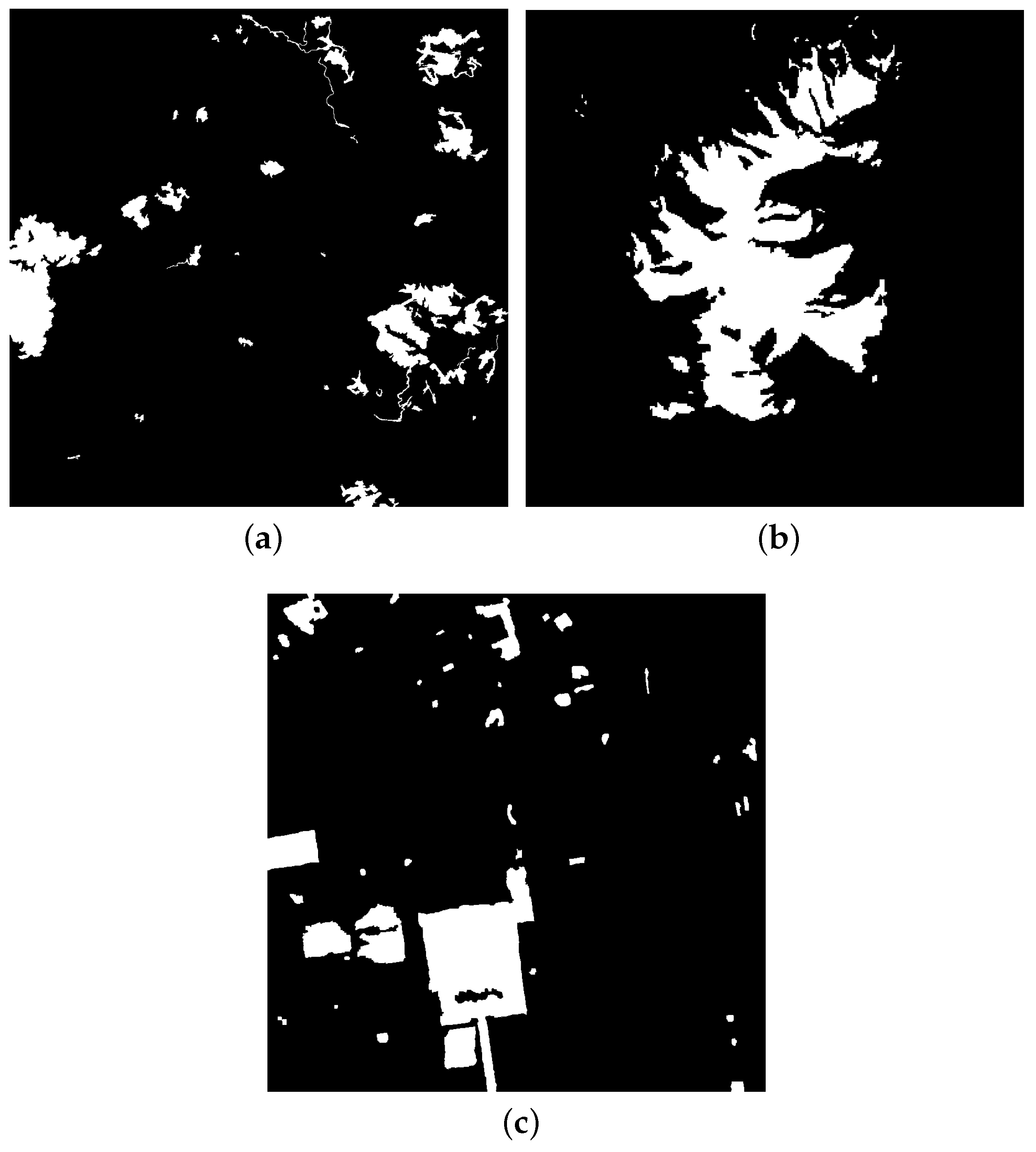
Figure 9.
Four PCA components of the QuickBird difference image and the selected PCs of TM and ASTER data. (a) the first PC for QuickBird images, ; (b) the second PC, ; (c) the third PC, ; (d) the fourth PC, ; (e) the selected component for TM images, ; and (f) the selected component for ASTER images, .

Figure 10.
(a–f) Change detection results for different approaches on the test data sets.


Table 1.
Normalized component selection index for three datasets.
| Dataset | Selected Component | ||||
|---|---|---|---|---|---|
| ASTER | 0.9991 | 0.0004 | 0.0005 | - | 1 |
| TM | 0.7291 | 0.1389 | 0.1320 | - | 1 |
| Quickbird | 0.0888 | 0.2375 | 0.5449 | 0.1288 | 2, 3 |
Table 2.
Error rate (), false-alarm rate () and missed-alarm rate () in percentage achieved by different change detection methods on the three data sets (Hobet, Mountain, Shijingshan).
Table 2.
Error rate (), false-alarm rate () and missed-alarm rate () in percentage achieved by different change detection methods on the three data sets (Hobet, Mountain, Shijingshan).
| Method | Hobet (TM) | Mountain (ASTER) | Shijingshan (QuickBird) | ||||||
|---|---|---|---|---|---|---|---|---|---|
| EM | 0.0346 | 0.0281 | 0.1181 | 0.0639 | 0.0741 | 0.0047 | 0.0809 | 0.0102 | 0.8051 |
| MRF | 0.0325 | 0.0323 | 0.0350 | 0.0626 | 0.0730 | 0.0046 | 0.0771 | 0.0021 | 0.8442 |
| BPCA | 0.0227 | 0.0020 | 0.2848 | 0.0196 | 0.0212 | 0.0098 | 0.0338 | 0.0061 | 0.3172 |
| MLSK | 0.0265 | 0.0004 | 0.3952 | 0.0165 | 0.0109 | 0.0493 | 0.0367 | 0.0008 | 0.4046 |
| PCA-RW | 0.0098 | 0.0035 | 0.0904 | 0.0137 | 0.0155 | 0.0031 | 0.0179 | 0.0070 | 0.1305 |
© 2017 by the authors. Licensee MDPI, Basel, Switzerland. This article is an open access article distributed under the terms and conditions of the Creative Commons Attribution (CC BY) license (http://creativecommons.org/licenses/by/4.0/).
Share and Cite
MDPI and ACS Style
Liu, Q.; Liu, L.; Wang, Y. Unsupervised Change Detection for Multispectral Remote Sensing Images Using Random Walks. Remote Sens. 2017, 9, 438. https://doi.org/10.3390/rs9050438
AMA Style
Liu Q, Liu L, Wang Y. Unsupervised Change Detection for Multispectral Remote Sensing Images Using Random Walks. Remote Sensing. 2017; 9(5):438. https://doi.org/10.3390/rs9050438
Chicago/Turabian StyleLiu, Qingjie, Lining Liu, and Yunhong Wang. 2017. "Unsupervised Change Detection for Multispectral Remote Sensing Images Using Random Walks" Remote Sensing 9, no. 5: 438. https://doi.org/10.3390/rs9050438
Note that from the first issue of 2016, this journal uses article numbers instead of page numbers. See further details here.