Revealing Implicit Assumptions of the Component Substitution Pansharpening Methods

Abstract

The component substitution (CS) pansharpening methods have been developed for almost three decades and have become better understood recently by generalizing them into one framework. However, few studies focus on the statistical assumptions implicit in the CS methods. This paper reveals their implicit statistical assumptions from a Bayesian data fusion framework and suggests best practices for histogram matching of the panchromatic image to the intensity image, a weighted summation of the multispectral images, to better satisfy these assumptions. The purpose of histogram matching was found to make the difference between the high-resolution panchromatic and intensity images as small as possible, as one implicit assumption claims their negligible difference. The statistical relationship between the high-resolution panchromatic and intensity images and the relationship between their corresponding low-resolution images are the same, as long as the low resolution panchromatic image is derived by considering the modulation transfer functions of the multispectral sensors. Hence, the histogram-matching equation should be derived from the low-resolution panchromatic and intensity images, but not derived from the high-resolution panchromatic and expanded low-resolution intensity images. Experiments using three example CS methods, each using the two different histogram-matching equations, was conducted on the four-band QuickBird and eight-band WorldView-2 top-of-atmosphere reflectance data. The results verified the best practices and showed that the histogram-matching equation derived from the high-resolution panchromatic and expanded low-resolution intensity images provides more-blurred histogram-matched panchromatic image and, hence less-sharpened pansharpened images than that derived from the low-resolution image pair. The usefulness of the assumptions revealed in this study for method developers is discussed. For example, the CS methods can be improved by satisfying the assumptions better, e.g., classifying the images into homogenous areas before pansharpening, and by changing the assumptions to be more general to address their deficiencies.

1. Introduction

Remotely-sensed images have exhibited explosive growth trends in multi-sensor, multi-temporal, and multi-resolution characteristics. However, there are contradictions between the resolution limitations of current remote sensing systems and the increasing need for high-spatial, high-temporal, and high-spectrum resolutions of satellite images [1,2,3]. One limitation is the spectral and spatial resolution tradeoff, e.g., more than 70% of current optical earth observation satellites simultaneously collect low spatial resolution (LR) multispectral and high spatial resolution (HR) panchromatic images. Pansharpening has been proposed to fuse a panchromatic and a multispectral image to generate a pansharpened multispectral image, which offers the detailed spatial information of panchromatic image and still preserves spectral characteristics [4]. When the spatial detail is obtained from multispectral and hyperspectral sequence, the pansharpening algorithm is called hypersharpening [5,6]. Detailed critical surveys of pansharpening algorithms can be found in [7,8,9], as well as a first comprehensive textbook [10]. Current pansharpening methods can generally be classified into component substitution (CS), multi-resolution analysis (MRA), and model-based methods. Recently, pansharpening is also formulated as a compressive sensing reconstruction problem, but this scheme has a significant computation complexity [11,12,13]. The MRA approaches extract high-pass spatial detail from the panchromatic image using spatial frequency filtering methods [14,15] and inject it into the multispectral bands interpolated at the resolution of the panchromatic image [10,16]. During the degradation process of the panchromatic, the sensor modulation transfer functions (MTF) are taken into account [8,17]. A simple modification of these schemes, also applicable to CS methods, replaces the interpolated multispectral image with its deblurred version, where the deblurring kernel is matched to the MTF of the multispectral sensor [18]. CS methods are attractive because they are fast and easy to implement [19]. The CS methods use the intensity-hue-saturation (IHS) [20], principal component analysis (PCA) [10], or Gram–Schmidt (GS) [10] transformation to project the multispectral reflectance/digit number (DN) images into another vector space, and replace a component in the new space with the histogram-matched panchromatic image. The pansharpened multispectral bands are derived by performing the inverse transformation to the original space, i.e., DN/reflectance.

Pioneered by [20], the CS methods are generalized into a new formulation [19,21] without explicit calculation of the forward and backward transformations. The new formulation includes (i) interpolating/expanding the multispectral image to the scale of the panchromatic image, (ii) calculating the intensity component, i.e., the component to be replaced in the new space, by summing up multispectral images with a set of weight coefficients, (iii) matching the histograms of the panchromatic image to the intensity component, and (iv) injecting the extracted details, i.e., the difference between the panchromatic and intensity images, after being modulated by a set of band-specific gain coefficients. The general scheme can describe any CS methods, including Brovey [10], depending on the values of the weight and gain coefficients (Table 1 in [19]). It is well known that CS methods suffer from spectral distortion originating from the spectral mismatch between the panchromatic and intensity images [19,22] and histogram matching in the above step (iii) is usually performed to reduce such mismatches [19,23].

The implicit statistical assumptions of the CS methods are not well understood, although the CS methods have been extensively studied [19,20,21,24], as described above. The purpose of this study is to reveal all of the implicit statistical assumptions in the CS methods, which can help to determine the suitability of the methods and help to improve methods by satisfying the assumptions better or by addressing the assumption deficiencies. This study treats the CS methods in the Bayesian data fusion framework [25,26,27,28,29,30,31,32] noticing that the original CS methods are performed in the vector space. Based on the reveled assumptions, best practices for the histogram matching in CS pansharpening are recommended and the usefulness of the assumptions in the methodology development is discussed.

This paper is organized as follows: In Section 2, all of the basic statistical assumptions of the CS methods are revealed by deriving the CS methods in a Bayesian data fusion framework and best practices of the histogram matching in CS pansharpening are suggested based on the assumptions; Section 3 reports the experimental results to confirm the analysis; Section 4 discusses these statistical assumptions; and Section 5 concludes the paper.

2. Concepts and Methodology

From a Bayesian perspective, images are represented in vector form (symbolized by a letter in bold and italics) and operations on images in matrix form (symbolized by a letter in bold). Consider the LR and HR images have n and N pixels, where N = r²n and r is the spatial resolution ratio. The desired HR multispectral image with k spectral bands in band-interleaved-by-pixel lexicographical notation is denoted as a vector, M = [M₁, M₂, …, M_N]^T, where M_j = [$M_j^1$, $M_j^2$, …, $M_j^k$] is the spectrum at the spatial location j (j = 1, 2, …, N) and $M_j^k$ is the kth multispectral band pixel value at the spatial location j. The HR panchromatic image is denoted as a vector with N elements, P = [P₁, P₂, …, P_N]^T, where P_j is the panchromatic pixel value at the spatial location j. In the CS methods:

$$\mathit{I}=B\mathit{M}+\mathit{\alpha }$$

(1)

where I is the HR intensity image vector with N elements, B is a weight coefficient matrix with N × Nk elements, M is the HR multispectral image vector with Nk elements, and α is a bias coefficient vector with N elements. The corresponding LR versions of M, P, and I are denoted as m, p, and i, respectively. The expanded images of m, p, and i having the same spatial scale as P are denoted as $\tilde{m}$, $\tilde{p}$, and ĩ, respectively. Similar to M_j, $\tilde{m}$_j = [${\tilde{m}}_j^1$, ${\tilde{m}}_j^2$, …, ${\tilde{m}}_j^k$] is the spectrum at location j. $\widehat{\mathit{M}}$ and $\widehat{{\mathit{M}}_j}$ denote the pansharpened image and pansharpened jth pixel spectrum, respectively.

2.1. Bayesian Fusion Framework

Bayesian data fusion treats the LR multispectral image m, HR panchromatic image P and HR multispectral image M as random vectors, and the solution can be derived by maximizing the conditional probability density function prob(M|P,m) [26,27,28,29,30]. Applying the Bayes rule:

$$prob(\mathit{M}|\mathit{P},\mathit{m})=prob\left(\mathit{M}\right)prob\left(\mathit{P}\left|\mathit{M}\right)prob(\mathit{m}|\mathit{M}\right)/prob\left(\mathit{P},\mathit{m}\right)$$

(2)

where prob(x|y) is the conditional probability density function of x given y, prob(M) is a prior probability density function of the vector M, prob(P,m) is the probability density function of the co-occurrence of vector P and m. Since prob(P,m) is not a function of M, we have:

$$prob(\mathit{M}|\mathit{P},\mathit{m})\propto prob\left(\mathit{M}\right)prob\left(\mathit{P}\left|\mathit{M}\right)prob(\mathit{m}|\mathit{M}\right)$$

(3)

Thus, the key to solve Equation (3) is to find the explicit expressions of the three probability density functions, prob(M), prob(P|M), and prob(m|M).

Assumption 1.

To derive prob(M), the difference vector between the HR and expanded LR multispectral image vectors, $\tilde{m}$ − M, is assumed to be a Gaussian vector with zero mean, then:

$$prob\left(\mathit{M}\right)={\left(2\pi \right)}^{-\frac{Nk}{2}}{\left({\mathit{C}}_{\mathit{M}}\right)}^{-\frac{1}{2}}exp\{-\frac{1}{2}{(\tilde{\mathit{m}}-\mathit{M})}^T{\mathit{C}}_{\mathit{M}}^{-1}(\tilde{\mathit{m}}-\mathit{M})\}$$

(4)

where N and k are the numbers of HR multispectral pixels and bands, respectively, C_M is the covariance matrix of the vector ($\tilde{m}$ − M) with Nk × Nk elements, and $\tilde{m}$ is the expanded multispectral image from LR multispectral image m.

Assumption 2.

To derive prob(P|M), the spectral mismatch image P − I is assumed to be a Gaussian vector with zero mean, then:

$$prob(\mathit{P}|\mathit{M})={\left(2\pi \right)}^{-\frac{N}{2}}{\left({\mathit{C}}_{\mathit{e}}\right)}^{-\frac{1}{2}}exp\{-\frac{1}{2}{\left(\mathit{P}-\mathit{I}\right)}^T{\mathit{C}}_{\mathit{e}}^{-1}\left(\mathit{P}-\mathit{I}\right)\}$$

(5)

where N is the number of HR multispectral pixels, C_e is the covariance matrix of vector P − I with N × N elements, and P and I are the HR panchromatic and intensity image vectors.

Assumption 3.

The contribution of the term prob(m|M), which can be used to guarantee that the pansharpened images $\widehat{\mathit{M}}$ are spectrally consistent to the observed LR multispectral images m, is negligible. It should be noted that this assumption is necessary to derive the CS methods formulation. It implies that CS methods are not strictly spectrally consistent, which is verified in the Section 3.3 and discussed in the Section 4.1

Combining Equations (3)–(5) and neglecting the term prob(m|M), the closed-form solution $\widehat{\mathit{M}}$ is [25,28]:

$$\widehat{\mathit{M}}=\tilde{\mathit{m}}+C_{\mathit{M}}{B}^{\mathrm{T}}{\left(C_{\mathit{e}}+B{C}_{\mathit{M}}{B}^{\mathrm{T}}\right)}^{-1}\left(\mathit{P}-\mathit{i}̃\right)$$

(6)

where $\tilde{m}$ is the expanded LR multispectral image, C_M is the covariance matrix of the vector ($\tilde{m}$ − M) first introduced in Equation (4), B is the weight coefficient matrix first introduced in Equation (1), C_e is the covariance matrix of vector P − I first introduced in Equation (5), and ĩ is the expanded intensity image:

$$\mathit{i}̃=B\tilde{\mathit{m}}+\mathit{\alpha }$$

(7)

where α is the bias coefficient vector first introduced in Equation (1).

Assumption 4.

To make this solution doable, all pixels are assumed to share the common weight and bias coefficients. Hence:

$$\mathit{\alpha }={\left[\alpha ,\alpha ,\dots ,\alpha \right]}_N$$

(8)

where α is the bias coefficient vector with N elements first introduced in Equation (1) and α is the common bias coefficient value.

$$\mathit{B}=diag{\left[\mathit{\beta },\mathit{\beta },\dots ,\mathit{\beta }\right]}_N={\left[\begin{array}{cccc}\mathit{\beta }& \mathbf{0}& \dots & \mathbf{0}\\ \mathbf{0}& \mathit{\beta }& \dots & \mathbf{0}\\ ⋮& ⋮& \ddots & ⋮\\ \mathbf{0}& \mathbf{0}& \dots & \mathit{\beta }\end{array}\right]}_N$$

(9)

where B is the weight coefficient matrix first introduced in Equation (1) and is a special type of block matrix derived as the direct sum (diag operator) of N duplicate vector β = [β¹, β², …, β^k], 0 is a k-element zero vector, β¹, β², …, β^k are the common spectral band weight coefficients, and N is the number of HR pixels.

Assumption 5.

A further assumption is that all the pixel values in the two difference vectors ($\tilde{m}$ − M) and (P − I) are independent and identically distributed (i.i.d.). In such a way that:

$${\mathit{C}}_{\mathit{e}}=diag{\left[{\sigma }_e^2,{\sigma }_e^2,\dots ,{\sigma }_e^2\right]}_N$$

(10)

$${\mathit{C}}_{\mathit{M}}=diag{\left[{\mathit{C}}_s,{\mathit{C}}_s,\dots ,{\mathit{C}}_s\right]}_N$$

(11)

where diag is the matrix direct sum operation as defined in Equation (9), ${\sigma }_e^2$ is the variance of all the pixels in image (P − I) and C_s is a spectral band covariance matrix with k × k elements:

$${\mathit{C}}_s=\left[\begin{array}{cccc}cov\left({\mathit{M}}^1,{\mathit{M}}^1\right)& cov\left({\mathit{M}}^1,{\mathit{M}}^2\right)& \dots & cov\left({\mathit{M}}^1,{\mathit{M}}^k\right)\\ cov\left({\mathit{M}}^2,{\mathit{M}}^1\right)& cov\left({\mathit{M}}^2,{\mathit{M}}^2\right)& \dots & cov\left({\mathit{M}}^2,{\mathit{M}}^k\right)\\ ⋮& ⋮& \ddots & ⋮\\ cov\left({\mathit{M}}^k,{\mathit{M}}^1\right)& cov\left({\mathit{M}}^k,{\mathit{M}}^2\right)& \dots & cov\left({\mathit{M}}^k,{\mathit{M}}^k\right)\end{array}\right]$$

(12)

where cov(x,y) is the covariance of two vectors x and y, M^k = [$M_1^k$, $M_2^k$, …, $M_N^k$] represents the kth HR multispectral band image vector with N elements with $M_j^k$being the kth multispectral band pixel value at the HR spatial location j.

Assumption 6.

The LR panchromatic image p is assumed being derived from the HR panchromatic P in the same way that m derived from M. This means that the MTF of the multispectral sensors reflecting the relationship between the LR and HR multispectral image (m and M) must be considered to derive p from P. Consequently, due to the assumption of the independent and identical distribution of HR pixels (Assumption 5) in P and M, the LR pixels in p and m are also independent and identically distributed and have the same distributions with their corresponding HR pixels. Hence, ${\sigma }_e^2$ can be estimated from (p − i) and cov(M^k, M^k) from m, i.e.:

$${\sigma }_e^2={{\displaystyle \sum }}_1^n{\left(p_j-i_j\right)}^2/n$$

(13)

where n is the number of the LR multispectral pixels, and p_j and i_j are the jth LR panchromatic and intensity image pixel values, respectively.

and:

$$cov\left({\mathit{M}}^x,{\mathit{M}}^y\right)=cov\left({\mathit{m}}^x,{\mathit{m}}^y\right) x=1,2,\dots ,k;y=1,2,\dots ,k$$

(14)

where m^k = [$m_1^k$, $m_2^k$, …, $m_n^k$] represents the kth LR multispectral band image vector with n elements with $m_j^k$ being the kth multispectral band pixel value at the LR spatial location j, and k is the number of multispectral spectral bands.

The large equation system in Equation (6) can then be spatially decomposed into pixel level equations:

$${\widehat{\mathit{M}}}_j={\tilde{\mathit{m}}}_{\mathit{j}}+{\mathit{g}}^T\left(P_{\mathit{j}}-{ĩ}_{\mathit{j}}\right)$$

(15)

$${\mathit{g}}^T=C_S{\mathit{\beta }}^T/\left({\sigma }_e^2+\mathit{\beta }{C}_S{\mathit{\beta }}^T\right)$$

(16)

where $\widehat{{\mathit{M}}_j}$ and $\tilde{m}$_j are the pansharpened and expanded multispectral spectra at location j, respectively, g is a gain coefficient vector with k elements, the super script T means the transpose of a vector, P_j and ĩ_j are the HR panchromatic and expanded intensity values at location j, respectively, and definitions of C_s, β, and ${\sigma }_e^2$ refer to the previous Equations (10), (12), and (13).

2.2. CS Methods from a Bayesian Perspective

Alternative Assumption 2. Equation (15) can be shrunk into the GS-based methods by assuming there is no spectral mismatch, i.e., ${\sigma }_e^2$ = 0 in Assumption 2 and the HR panchromatic image P is perfectly matched with the intensity image I. This is based on the linear transformation and sum properties of the covariance:

$${\mathit{g}}_{GS}^T=\left[cov\left({\mathit{m}}^1,\mathit{i}\right)/{\sigma }_{\mathit{i}}^2, cov\left({\mathit{m}}^2,\mathit{i}\right)/{\sigma }_{\mathit{i}}^2,\dots ,cov\left({\mathit{m}}^k,\mathit{i}\right)/{\sigma }_i^2\right]=C_s{\mathit{\beta }}^T/\mathit{\beta }{C}_s{\mathit{\beta }}^T$$

(17)

where g_GS is the GS gain coefficient vector defined in Table 1 in [19], ${\sigma }_i^2$ is the variance of the intensity image i and $cov\left({\mathit{m}}^x,\mathit{i}\right)$ is the covariance between the xth band LR multispectral image m^x and the LR intensity image i.

For the GS method, the weight and the gain coefficients satisfy:

$$\mathit{\beta }{\mathit{g}}_{GS}^T=\mathit{\beta }{C}_s{\mathit{\beta }}^T{\left[\mathit{\beta }{C}_s{\mathit{\beta }}^T\right]}^{-1}=1$$

(18)

This property has been mentioned in [33]. From Table 1 in [19], it is easy to prove that this equation is satisfied by the IHS, generalized IHS (GIHS) and Brovey methods. The PCA method also satisfies this equation as the PCA gain and weights coefficients are the same and from a column of a unitary matrix created by PCA.

2.3. Best Practices in Histogram Matching

The spectral difference between the HR intensity I and panchromatic P images, i.e., ${\sigma }_e^2$ value, should be minimized to satisfy the no spectral mismatch assumption (Alternative Assumption 2) as much as possible. Several methods have been introduced to minimize ${\sigma }_e^2$ including histogram matching of the panchromatic image P to the intensity image I and deriving the best intensity image with weight coefficients derived from the multivariate regression between the multispectral and panchromatic images [19]. The conception of histogram matching is to make a virtual observed panchromatic image, P_hist, that is statistically (mean and standard deviation) similar to the intensity image I. However, the target image that the observed panchromatic image P should be histogram matched to, i.e., the HR intensity image I, is unavailable. Recall the independent and identical distribution assumption (Assumption 5) and the HR image pair histogram matching equation can be derived from their LR image pair (Equations (13) and (14)). Consequently, the pixel value in P is histogram-matched using the equation derived from the LR panchromatic p and intensity image i:

$${\mathit{P}}_{hist}\left(\mathit{P}\to \mathit{I}\right)={\mathit{P}}_{hist}\left(\mathit{p}\to \mathit{i}\right)=\left(\mathit{P}-mean\left(\mathit{p}\right)\right)\sqrt{\frac{cov\left(\mathit{i},\mathit{i}\right)}{cov\left(\mathit{p},\mathit{p}\right)}}+mean\left(\mathit{i}\right)$$

(19)

where P_hist(P→I) and P_hist(p→i) are the histogram-matched HR panchromatic images using the equations from the LR image pair and the HR image pair, respectively, and mean and cov represent the mean and covariance operations, respectively. Histogram matching directly from P to ĩ, P_hist(P→ĩ), is not proper as the statistical relationship between the HR panchromatic image P and intensity image I is not the same as that between the HR panchromatic image P and the expanded intensity image ĩ:

$${\mathit{P}}_{hist}\left(\mathit{P}\to \mathit{I}\right)\ne {\mathit{P}}_{hist}\left(\mathit{P}\to \mathit{i}̃\right)=\left(\mathit{P}-mean\left(\mathit{P}\right)\right)\sqrt{\frac{cov\left(\mathit{i}̃,\mathit{i}̃\right)}{cov\left(\mathit{P},\mathit{P}\right)}}+mean(\mathit{i}̃)$$

(20)

where P_hist(P→I) has been defined in Equation (19), P_hist(P→ĩ) is the histogram-matched HR panchromatic image using the equation from HR panchromatic image P and expanded intensity image ĩ, mean and cov represent the mean and covariance operations, respectively. Although the mean values of p and P are the same, their variance values could be largely different due to the scale difference [34,35]. The difference between P and ĩ includes not only the residual ${\sigma }_i^2$, but also the spatial details to be injected, P − ĩ = (P − $\tilde{p}$) + ($\tilde{p}$ − ĩ), where P − $\tilde{p}$ is the spatial details to be injected and ($\tilde{p}$ − ĩ) can be interpreted as the spectral mismatch (residual ${\sigma }_i^2$) between the panchromatic and intensity images.

Due to the Assumption 6, the LR panchromatic image p should be derived from the HR panchromatic image P in the same way that the LR multispectral image m derived from the HR multispectral image M (i.e., taking care of the multispectral sensor modulation transfer functions).

3. Experiments and Results

3.1. Data and Experimental Settings

The datasets used for this experiment include a rural area QuickBird image near Boulder City, CO, USA (Figure 1) acquired on 4 July 2005 and two urban area WorldView-2 (Figure 2 and Figure 3) images across San Clemente, CA, USA acquired on 21 March 2012. The rural area QuickBird image (Figure 1) is mainly covered by bare soil and vegetation with some urban buildings in the northeast corner area and has 2400 × 2400 0.6-m panchromatic and 600 × 600 2.4-m multispectral pixels. The QuickBird multispectral image consists of four bands, including blue, 450–520 nm, green, 520–600 nm, red, 630–690 nm and near infrared (NIR), 760–900 nm. The first urban area WorldView-2 image (Figure 2, hereafter referred to as WorldView-2 urban 1 dataset) is mainly covered by unban buildings, roads, and urban vegetation, and has 2048 × 2048 2.0-m multispectral pixels and 8192 × 8192 0.5-m panchromatic pixels. The second urban area WorldView-2 image (Figure 3, hereafter referred to as WorldView-2 urban 2 dataset) is a mixture of urban buildings and vegetation, which is a typical temperate urban landscape. It has 512 × 512 2.0-m multispectral pixels and 2048 × 2048 0.5-m panchromatic pixels. This additional urban dataset is used specifically to examine the method on the vegetation and building mixture typically exhibiting in high-resolution images. The WorldView-2 multispectral images have eight spectral bands: coastal blue, 400–450 nm; blue, 450–510 nm; green, 510–580 nm; yellow, 585–625 nm; red, 630–690 nm; red edge, 705–745 nm; NIR1, 770–895 nm; and NIR2, 860–1040 nm.

The QuickBird and WorldView-2 panchromatic and multispectral bands’ top-of-atmosphere (TOA) reflectance, derived from DN values using the coefficients provided in the metadata and method provided by [36], were used in the pansharpening experiments to reduce incoming solar irradiance and calibration gain variations among different bands in the DN values.

We conducted pansharpening at both reduced and full scales. At the reduced scale, the panchromatic and multispectral images are first degraded by four before pansharpening so that the original multispectral data could be used as references for the pansharpening result evaluation. Sensor modulation transfer functions (MTF) are taken into account during the degradation. The sensor MTF can be matched using Gaussian filters with parameters tuned using the values of the amplitude response at the Nyquist frequency depicting the MTF, commonly provided by the manufacturer as a sensor specification [8,17]. They are 0.35 and 0.27 for the first seven and the eighth multispectral bands for the WorldView-2 sensor, and 0.34, 0.32, 0.30, and 0.22 for the four QuickBird multispectral bands. Their corresponding Gaussian filters implemented in Matlab codes are provided by Vivone [8] available at http://openremotesensing.net/index.php/codes/11-pansharpening/2-pansharpening.

The two histogram matching equations (Equations (19) and (20)) were compared for the generalized IHS (GIHS), GS, and adaptive GS (GSA) [19] pansharpening all of the four multispectral bands of the QuickBird rural images and all of the eight multispectral bands of the two WorldView-2 urban images. These three CS methods are selected as they are commonly used in the literature [19,20] and have been proved with better performance than the other CS methods [19,37]. The GSA method is the same as the GS method except that the intensity image is synthesized by using the weight coefficients derived using regression between the multispectral and the degraded LR panchromatic images rather than using equal weight coefficients for each multispectral band image [19]. During the histogram matching and GSA regression coefficients derivation, the LR panchromatic image is derived by degrading panchromatic image by mimicking the multispectral sensor MTF so that the LR panchromatic and multispectral images are comparable (Assumption 6).

3.2. Quantitative Evaluation of the Experimental Results

The consistency and synthesis properties of the Wald’s protocol [38] were used as validation strategies. The consistency property has been proved effective in [38] and was used to validate the full scale experiments. To check the consistency property, the pansharpening images were first degraded using the sensor specific MTF as described in Section 3.1. The synthesis property can only be applied to the reduced scale experiment. Only the consistency property has been evaluated in the full scale experiments and other full scale evaluation methods [39], such as quality without reference (QNR) [35], were not used as the main purpose of this study is to check the spectral consistency of the pansharpened images induced by different strategies in the histogram matching. Three quantitative scores were used: (i) the first is the ERGAS index, from its French name “relative dimensionless global error in synthesis”, is a global radiometric value error index [10]. The best ERGAS value is zero; (ii) the second is the spectral angle mapper (SAM), which calculates the angle between two spectral vectors at each pixel and is averaged over the test image—the best value is zero; and (iii) the third ones are related to universal quality index (Q) index. For the four-band QuickBird image the Q4 index proposed by [40] was used, which is an extension of the universal quality index suitable for four-band multispectral images. For the eight-band WorldView-2 image, Q2ⁿ [41] was used, which is an extension of the Q4 index for any number of spectral bands. These two indices are sensitive to both correlation loss and spectral distortion between two multispectral images, and allow both spatial and spectral distortions to be combined in a unique parameter. The best value is one, with a range from zero to one. In this study, Q4 and Q2ⁿ were both calculated on 32 × 32 pixel blocks as suggested by the authors who proposed them.

In order to give a clear picture on the difference between the panchromatic and intensity images (i.e., the spectral mismatch), the $\sqrt{{\sigma }_e^2}$ values from Equation (13) are also calculated.

3.3. Results

Table 1. Average quality scores of the pansharpened four-band QuickBird rural dataset (Figure 1). The scores shown in bold indicate the better metric between the two results produced by the same pansharpening method (GIHS, GS, or GSA), but using two different histogram equations (P_hist(p→i) and P_hist(P→ĩ)).

	Synthesis Property at Reduced Scale				Consistency Property at Full Scale
Method	Q4	SAM	ERGAS	$\sqrt{{\mathit{\sigma }}_{\mathit{e}}^2}$	Q4	SAM	ERGAS	$\sqrt{{\mathit{\sigma }}_{\mathit{e}}^2}$
EXP ($\tilde{m}$)	0.630	4.440	4.627	NA	0.973	1.188	1.165	NA
GIHS Phist(p→i)	0.827	5.406	4.192	0.0051	0.973	1.899	2.115	0.0079
GIHS Phist(P→ĩ)	0.780	5.111	4.237	0.0071	0.966	1.696	2.228	0.0089
GS Phist(p→i)	0.850	4.801	3.929	0.0051	0.976	1.514	1.872	0.0079
GS Phist(P→ĩ)	0.805	4.680	4.076	0.0071	0.969	1.426	2.011	0.0089
GSA Phist(p→i)	0.853	4.491	3.608	0.0024	0.976	1.256	1.241	0.0068
GSA Phist(P→ĩ)	0.807	4.474	3.845	0.0074	0.967	1.276	1.494	0.0092

,

Table 2. Average quality scores of the pansharpened eight-band WorldView-2 urban 1 dataset (Figure 2). The scores shown in bold indicate the better metric between the two results produced by the same pansharpening method (GIHS, GS, or GSA), but using two different histogram equations (P_hist(p→i) and P_hist(P→ĩ)).

	Synthesis Property at Reduced Scale				Consistency Property at Full Scale
Method	Q4	SAM	ERGAS	$\sqrt{{\mathit{\sigma }}_{\mathit{e}}^2}$	Q4	SAM	ERGAS	$\sqrt{{\mathit{\sigma }}_{\mathit{e}}^2}$
EXP ($\tilde{m}$)	0.571	5.310	5.184	NA	0.733	1.745	1.526	NA
GIHS Phist(p→i)	0.607	5.563	3.540	0.0099	0.679	2.318	2.636	0.0145
GIHS Phist(P→ĩ)	0.583	5.730	3.821	0.0113	0.657	2.413	2.665	0.0146
GS Phist(p→i)	0.624	5.553	3.478	0.0099	0.667	2.646	2.485	0.0145
GS Phist(P→ĩ)	0.599	5.871	3.789	0.0113	0.649	2.822	2.523	0.0146
GSA Phist(p→i)	0.626	5.000	3.149	0.0023	0.764	1.807	1.828	0.0088
GSA Phist(P→ĩ)	0.592	5.335	3.542	0.0072	0.723	1.999	1.959	0.0097

and

Table 3. Average quality scores of the pansharpened eight-band WorldView-2 urban 2 dataset (Figure 3). The scores shown in bold indicate the better metric between the two results produced by the same pansharpening method (GIHS, GS, or GSA), but using two different histogram equations (P_hist(p→i) and P_hist(P→ĩ)).

	Synthesis Property at Reduced Scale				Consistency Property at Full Scale
Method	Q4	SAM	ERGAS	$\sqrt{{\mathit{\sigma }}_{\mathit{e}}^2}$	Q4	SAM	ERGAS	$\sqrt{{\mathit{\sigma }}_{\mathit{e}}^2}$
EXP ($\tilde{m}$)	0.317	6.545	5.458	NA	0.557	2.051	1.542	NA
GIHS Phist(p→i)	0.341	6.679	3.797	1.266	0.465	2.495	2.924	1.7855
GIHS Phist(P→ĩ)	0.303	6.688	4.291	1.414	0.398	2.508	2.929	1.7876
GS Phist(p→i)	0.362	6.501	3.725	1.266	0.434	2.766	2.657	1.7855
GS Phist(P→ĩ)	0.308	6.648	4.287	1.414	0.385	2.838	2.684	1.7876
GSA Phist(p→i)	0.356	6.350	3.209	0.243	0.636	2.123	1.882	0.9771
GSA Phist(P→ĩ)	0.320	6.436	3.930	0.980	0.550	2.209	2.088	1.1309

show quantitative scores for the synthesis property at the reduced scale (columns on the left side of the tables) and for the consistency property at the full scale (columns on the right side of the tables) for the QuickBird rural (Table 1) and WorldView-2 urban 1 (Table 2) and 2 (Table 3) datasets. $\sqrt{{\sigma }_e^2}$ is also tabulated in all of the tables. ‘EXP’ in these tables represents the plain expanded resampling of the multispectral dataset at the scale of the panchromatic, i.e., $\tilde{m}$. All of the CS pansharpening methods have relatively low ${\sigma }_e^2$ values (less than 0.02 in top-of-atmosphere reflectance units) indicating that the histogram matching effectively reduce the radiometric difference between the intensity and panchromatic images. This number is smaller than the top of atmosphere reflectance noise effect induced by the atmospheric scattering and by the sun-sensor-target geometry [42]. The GIHS and GS methods have the same ${\sigma }_e^2$ values as they have the same intensity image derived using an equal weight coefficient for each multispectral band image. The GSA method produced smaller ${\sigma }_e^2$ values than the GS method as the design of the GSA has minimized the spectral mismatch between the LR intensity image i and LR panchromatic image p [19]. The ${\sigma }_e^2$ values are greater for the full scale pansharpening than that for the reduced scale pansharpening for all of the same methods and the same datasets. This could be because, at the full scale experiments, there is still some mismatch between the real multispectral sensor MTF and the MTF used for degrading the panchromatic image (i.e., MTF provided by the manufacturer) due to the on-orbit sensor degradation. To obtain a more reliable sensor MTF, on-orbit estimation of the sensor point spread function is needed [43].

Comparing the pansharpened results using the histogram-matched panchromatic image with Equation (19) (P_hist(p→i)) and with Equation (20) (P_hist(P→ĩ)), the P_hist(p→i) in Equation (19) always performs better for all of the quantitative scores for the WorldView-2 urban dataset and has smaller ${\sigma }_e^2$ values. There are a few exceptions where P_hist(P→ĩ) in Equation (20) performs slightly better (e.g., the SAM metric of the synthesis property the GSA method) in the QuickBird rural dataset. This experimentally confirmed our analysis that the histogram-matched equation should be derived from the LR intensity and panchromatic image pairs. The SAM exceptions in the QuickBird dataset could be because the SAM metric is more robust to noise when the vector dimension it measures is larger. The QuickBird images only have four multispectral bands, which make the SAM metric sensitive to the radiometric distortion in the multispectral bands. For example, a small improper injection on the blue band of the QuickBird image, due to the less overlapping between the blue and panchromatic bands, could cause large errors in the SAM values.

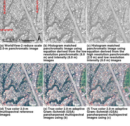
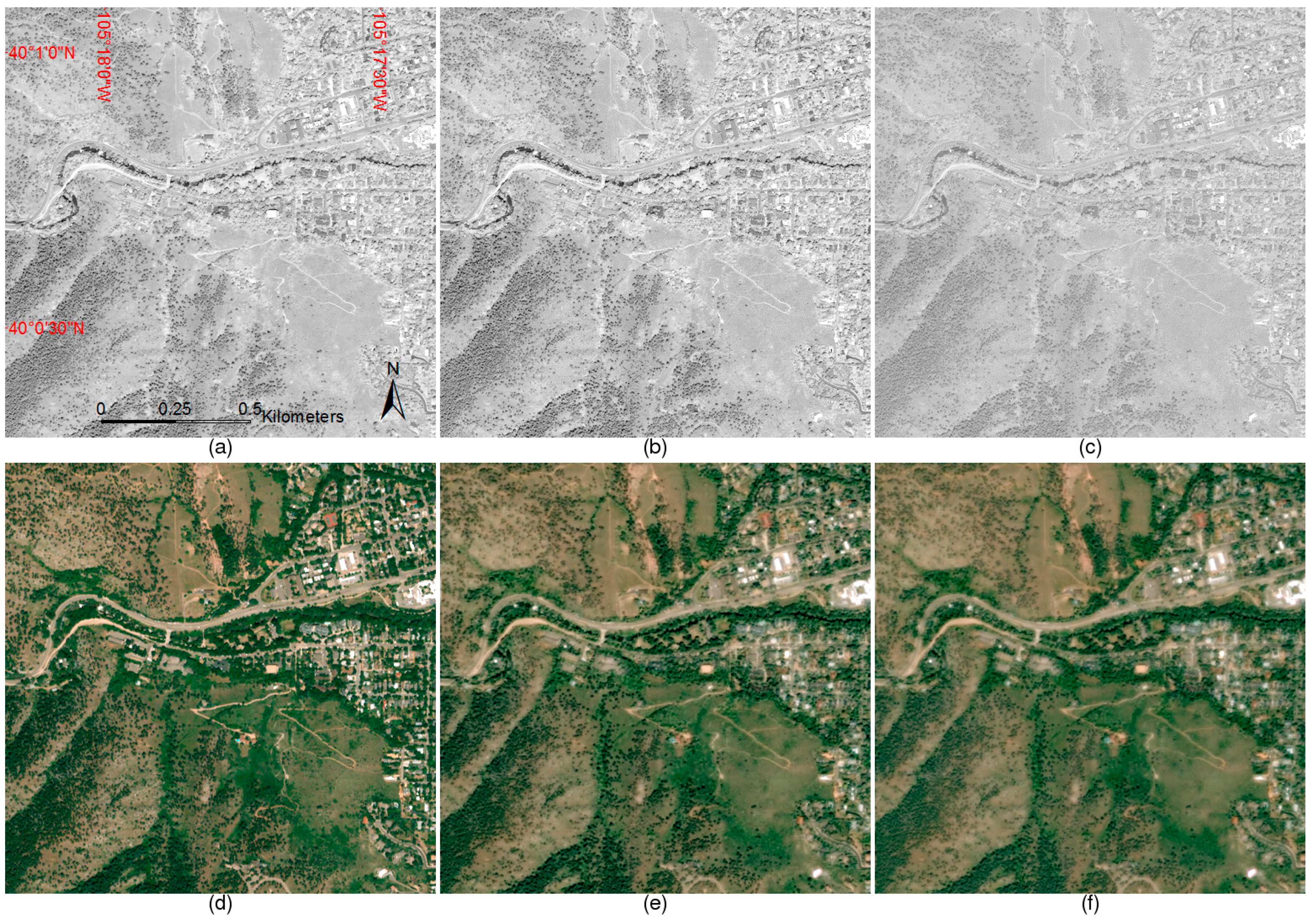
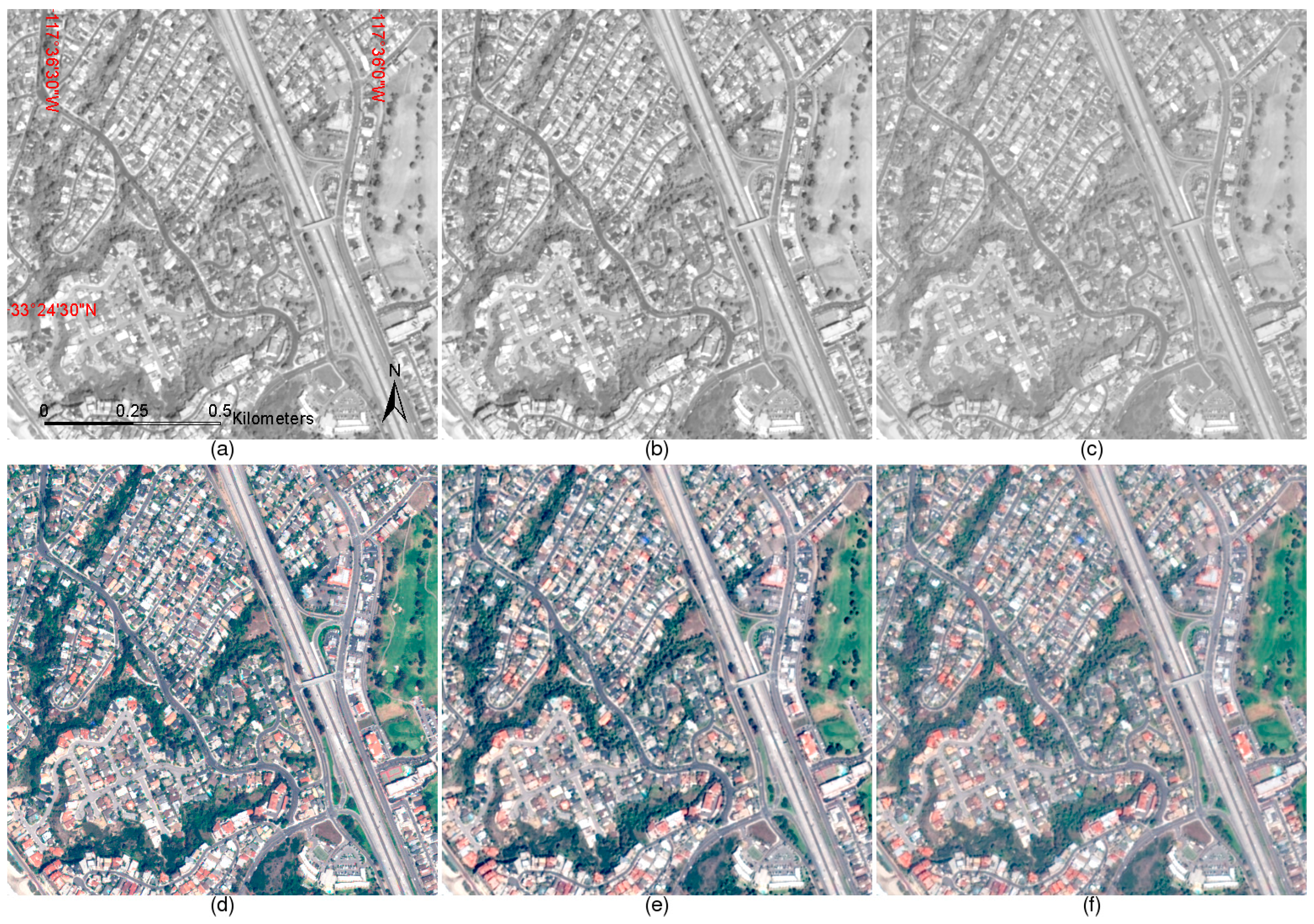
Figure 1, Figure 2 and Figure 3 show the panchromatic (Figure 1a, Figure 2a and Figure 3a) and two histogram matched panchromatic images (Figure 1b,c, Figure 2b,c, Figure 3b,c) with the same contrast stretch, and true color reference (Figure 1d, Figure 2d and Figure 3d) and pansharpened multispectral top of atmosphere reflectance images from the GSA method (Figure 1e,f, Figure 2e,f, Figure 3e,f) using two different histogram-matching equations with the same contrast stretch. Only the results from the GSA method are shown to save space since the GSA method performed the best. Clearly, histogram matching the panchromatic image using the equation provided by the HR panchromatic and the expanded intensity image pair (P_hist(P→ĩ), Figure 1c, Figure 2c, and Figure 3c) has less spatial detail than that using the equation from the LR intensity and panchromatic image pair (P_hist(p→i), Figure 1b, Figure 2b, and Figure 3b). This is reasonable as the purpose of histogram matching is to adjust the mean and variance of the original image (i.e., LR or HR panchromatic images, p or P, in this case) to the same as the target image (i.e., LR panchromatic intensity image i or its expanded version ĩ in this case). The P_hist(P→ĩ) has less spatial detail because it has a lower variance since the LR panchromatic image p has a lower variance compared to the HR panchromatic image P [34,35]. Comparing the two different pansharpened images and original multispectral images show clearly less sharpening detail in the QuickBird rural dataset and slight spectral distortion in the two WorldView-2 urban datasets for the pansharpened images using the directly-histogram-matched panchromatic band P_hist(P→ĩ) in Equation (20).

4. Discussion

4.1. The Usefulness of the Revealed Statistical Assumptions

It should be noted that the statistical assumptions are not proposed by the authors. However, they are revealed by us to better understand the implicit assumptions that are made by the CS methods. This is useful for the CS method development, e.g., as illustrated in this study for the best histogram matching method suggestion. Some other possible uses for the method development are discussed below, which requires further research.

One assumption is that the spectral consistency term prob(m|M) is neglected in Equation (2), which results in the pansharpened images not being strictly spectrally consistent. This has been shown in Table 1, Table 2 and Table 3 where no pansharpened images are perfectly spectrally consistent with the original multispectral images. Facilitated by the flexibility of the extension of the Bayesian data fusion framework, studies have tried to add this term at the price of a more complicated solution [25]. This is because the point spread function (i.e., MTF) used in the spectral consistency term will make spatially decomposing the large equation system of Equation (6) into pixel level equation, such as Equation (15), impossible [25]. A detailed analysis of the contribution of this term is illustrated in [25].

Another assumption is that the difference between the LR and HR multispectral image vectors ($\tilde{m}$ − M) is a Gaussian vector with zero mean. Perhaps other models of distribution, such as multimodal distribution, are more suitable to represent this difference. Within the Bayesian framework and the deduction process in this paper, one can just replace the Gaussian distribution with a novel multimodal distribution and derive its solution to design new CS methods.

Another assumption is that all the pixels in the difference vector between the LR and HR multispectral images ($\tilde{m}$ − M) and in the difference vector between the HR panchromatic and intensity images (P − I) are independent and identically distributed. Apparently, due to the spatial heterogeneity nature of the earth surface, the validity of this assumption is really subject to the extent and location of the study area. However, restricting this assumption in a spatial homogenous area is always a better option. To this aim, some authors have improved CS methods by restricting this assumption in a local sliding window [44,45,46], in a group of homogenous pixels after image classification [47,48], or paying attention to the mixed pixels [49].

4.2. Time Complexity of the Suggested Histogram Matching Method

The computational efficiency of the different pansharpening methods using the two different histogram-matching equations was measured by counting the run time of each method for each study image at the reduced scale experiments. The run time measurements excluded the image reading and writing operations. All of the code was written in the Matlab language and run using an Intel^® Xeon^® Processor X3450 (4 cores, 8 M Cache, 2.66 GHz) CPU with 8.00 GB of memory and the 64-bit Windows 7 operating system.

Table 4. Run time (in seconds) of each method for the three datasets.

Method	4-Band QuickBird Dataset (Figure 1)	8-Band WorldView-2 Urban 1 Dataset (Figure 2)	8-Band WorldView-2 Urban 2 Dataset (Figure 3)
EXP ($\tilde{m}$)	0.11	0.56	0.22
GIHS Phist(p→i)	0.31	5.98	0.47
GIHS Phist(P→ĩ)	0.26	5.10	0.37
GS Phist(p→i)	0.37	6.49	0.50
GS Phist(P→ĩ)	0.29	5.17	0.41
GSA Phist(p→i)	0.40	6.52	0.55
GSA Phist(P→ĩ)	0.41	6.50	0.56

shows the run time of each method for all three datasets. The benchmark plain expanded/resampling algorithm is computationally the most efficient, with run times of less than 0.6 s for all three datasets. The additional step of derivation of the LR panchromatic images for the suggested histogram matching is not very time consuming for the GIHS and CS methods. The GIHS and CS methods using the suggested histogram matching are only 17–27% more than those using the histogram-matching equation provided by the HR panchromatic and resampled LR intensity images. This can be mitigated by the development of hardware computation capabilities or by using advanced paralleling algorithms [50]. Furthermore, the run time of the GSA method using the suggested histogram matching is slightly less than those using the histogram matching with the equation provided by the HR panchromatic and resampled LR intensity images. This is because (i) the GSA method needs the LR panchromatic image for the optimal weights determination in intensity image derivation no matter what histogram matching is used; and (ii) using LR images in Equation (19) with n pixels saves some time, as opposed to using the HR images in Equation (20) with N pixels (16 times greater than n in our study) for histogram matching.

5. Conclusions

In this paper, the implicit statistical assumptions of the CS pansharpening methods are revealed by interpreting them from the Bayesian data fusion framework. Best practices for histogram matching of the HR panchromatic image to the intensity image are suggested to better satisfy the implicit assumptions. The HR panchromatic image should be histogram matched using the equation derived from the LR panchromatic and intensity images instead of using equations derived from the HR panchromatic and expanded LR intensity images. This is because (i) one assumption suggests the negligible difference between the HR intensity and panchromatic images; and (ii) the relationship between the HR intensity and panchromatic images is comparable to the relationship between the LR intensity and panchromatic images provided the LR panchromatic image is derived from the HR panchromatic image by considering the multispectral sensor modulation transfer functions. We tested the two different histogram-matching equations using the GIHS, GS, and adaptive GS (GSA) methods on both QuickBird and WorldView-2 top-of-atmosphere reflectance images and proved that the suggested histogram-matching equation is effective. The usefulness of the statistical assumptions revealed in this study for method developers is discussed. For example, none of the CS methods can produce pansharpened images spectrally consistent to the LR multispectral images since the implicit Assumption 1 omits the spectral consistency term. Classifying the images into homogenous areas before pansharpening can make Assumption 5 be better satisfied, i.e., all of the pixels in the difference vector between the LR and HR multispectral images ($\tilde{m}$ − M) and in the difference vector between the HR panchromatic and intensity images (P − I) are independent and identically distributed.

References

- Zhang, Y.; Roshan, A.; Jabari, S.; Khiabani, S.A.; Fathollahi, F.; Mishra, R.K. Understanding the quality of pansharpening—A lab study. Photogramm. Eng. Remote Sens. 2016, 82, 747–755. [Google Scholar] [CrossRef]
- Gao, F.; Hilker, T.; Zhu, X.; Anderson, M.; Masek, J.; Wang, P.; Yang, Y. Fusing Landsat and MODIS data for vegetation monitoring. IEEE Geosci. Remote Sens. Mag. 2015, 3, 47–60. [Google Scholar] [CrossRef]
- Garzelli, A. A review of image fusion algorithms based on the super-resolution paradigm. Remote Sens. 2016, 8, 797. [Google Scholar] [CrossRef]
- Wald, L. Some terms of reference in data fusion. IEEE Trans. Geosci. Remote Sens. 1999, 37, 1190–1193. [Google Scholar] [CrossRef]
- Selva, M.; Aiazzi, B.; Butera, F.; Chiarantini, L.; Baronti, S. Hyper-sharpening: A first approach on SIM-GA data. IEEE J. Sel. Top. Appl. Earth Obs. Remote Sens. 2015, 8, 3008–3024. [Google Scholar] [CrossRef]
- Loncan, L.; Almeida, L.B.; Bioucas-Dias, J.M.; Briottet, X.; Chanussot, J.; Dobigeon, N.; Fabre, S.; Liao, W.; Licciardi, G.A.; Simoes, M.; et al. Hyperspectral pansharpening: A review. IEEE Geosci. Remote Sens. Mag. 2015, 3, 27–46. [Google Scholar] [CrossRef]
- Thomas, C.; Ranchin, T.; Wald, L.; Chanussot, J. Synthesis of multispectral images to high spatial resolution: A critical review of fusion methods based on remote sensing physics. IEEE Trans. Geosci. Remote Sens. 2008, 46, 1301–1312. [Google Scholar] [CrossRef]
- Vivone, G.; Alparone, L.; Chanussot, J.; Mura, M.D.; Garzelli, A.; Licciardi, G.A.; Restaino, R.; Wald, L. A critical comparison among pansharpening algorithms. IEEE Trans. Geosci. Remote Sens. 2015, 53, 2565–2586. [Google Scholar] [CrossRef]
- Schmitt, M.; Zhu, X.X. Data fusion and remote sensing: An ever-growing relationship. IEEE Geosci. Remote Sens. Mag. 2016, 4, 6–23. [Google Scholar] [CrossRef]
- Alparone, L.; Aiazzi, B.; Baronti, S.; Garzelli, A. Remote Sensing Image Fusion; CRC Press: Boca Raton, FL, USA, 2015. [Google Scholar]
- Li, S.; Yang, B. A new pan-sharpening method using a compressed sensing technique. IEEE Trans. Geosci. Remote Sens. 2011, 49, 738–746. [Google Scholar] [CrossRef]
- Zhu, X.X.; Grohnfeldt, C.; Bamler, R. Exploiting Joint Sparsity for Pansharpening: The J-SparseFI Algorithm. IEEE Trans. Geosci. Remote Sens. 2016, 54, 2664–2681. [Google Scholar] [CrossRef]
- Li, J.; Yuan, Q.; Shen, H.; Zhang, L. Noise Removal from Hyperspectral Image with Joint Spectral—Spatial Distributed Sparse Representation. IEEE Trans. Geosci. Remote Sens. 2016, 54, 5425–5439. [Google Scholar] [CrossRef]
- Zhang, D.; You, X.; Wang, P.S.; Yanushkevich, S.N.; Tang, Y.Y. Facial biometrics using nontensor product wavelet and 2D discriminant techniques. Int. J. Pattern Recognit. Artif. Intell. 2009, 23, 521–543. [Google Scholar] [CrossRef]
- You, X.; Du, L.; Cheung, Y.M.; Chen, Q. A blind watermarking scheme using new nontensor product wavelet filter banks. IEEE Trans. Image Process. 2010, 19, 3271–3284. [Google Scholar] [CrossRef] [PubMed]
- Zhang, Y.; Hong, G. An IHS and wavelet integrated approach to improve pan-sharpening visual quality of natural colour IKONOS and QuickBird images. Inf. Fusion 2005, 6, 225–234. [Google Scholar] [CrossRef]
- Aiazzi, B.; Alparone, L.; Baronti, S.; Garzelli, A.; Selva, M. MTF-tailored multiscale fusion of high-resolution MS and pan imagery. Photogramm. Eng. Remote Sens. 2006, 72, 591–596. [Google Scholar] [CrossRef]
- Palsson, F.; Sveinsson, J.R.; Ulfarsson, M.O.; Benediktsson, J.A. MTF-Based Deblurring Using a Wiener Filter for CS and MRA Pansharpening Methods. IEEE J. Sel. Top. Appl. Earth Obs. Remote Sens. 2016, 9, 2255–2269. [Google Scholar] [CrossRef]
- Aiazzi, B.; Baronti, S.; Selva, M. Improving component substitution pansharpening through multivariate regression of MS plus Pan data. IEEE Trans. Geosci. Remote Sens. 2007, 45, 3230–3239. [Google Scholar] [CrossRef]
- Tu, T.-M.; Su, S.-C.; Shyu, H.-C.; Huang, P.S. A new look at IHS-like image fusion methods. Inf. Fusion 2001, 2, 177–186. [Google Scholar] [CrossRef]
- Dou, W.; Chen, Y.; Li, X.; Sui, D.Z. A general framework for component substitution image fusion: An implementation using the fast image fusion method. Comput. Geosci. 2007, 33, 219–228. [Google Scholar] [CrossRef]
- Xu, Q.; Li, B.; Zhang, Y.; Ding, L. High-fidelity component substitution pansharpening by the fitting of substitution data. IEEE Trans. Geosci. Remote Sens. 2014, 52, 7380–7392. [Google Scholar]
- Jelének, J.; Kopačková, V.; Koucká, L.; Mišurec, J. Testing a modified PCA-based sharpening approach for image fusion. Remote Sens. 2016, 8, 794. [Google Scholar] [CrossRef]
- Aiazzi, B.; Alparone, L.; Baronti, S.; Carlà, R.; Garzelli, A.; Santurri, L. Sensitivity of pansharpening methods to temporal and instrumental changes between multispectral and panchromatic data sets. IEEE Trans. Geosci. Remote Sens. 2016, 55, 308–319. [Google Scholar] [CrossRef]
- Zhang, H.K.; Huang, B. A new look at image fusion methods from a Bayesian perspective. Remote Sens. 2015, 7, 6828–6861. [Google Scholar] [CrossRef]
- Fasbender, D.; Radoux, J.; Bogaert, P. Bayesian data fusion for adaptable image pansharpening. IEEE Trans. Geosci. Remote Sens. 2008, 46, 1847–1857. [Google Scholar] [CrossRef]
- Zhang, Y.; Backer, S.D.; Scheunders, P. Noise-resistant wavelet-based Bayesian fusion of multispectral and hyperspectral images. IEEE Trans. Geosci. Remote Sens. 2009, 47, 3834–3843. [Google Scholar] [CrossRef]
- Eismann, M.T.; Hardie, R.C. Application of the stochastic mixing model to hyperspectral resolution enhancement. IEEE Trans. Geosci. Remote Sens. 2004, 42, 1924–1933. [Google Scholar] [CrossRef]
- Hardie, R.C.; Eismann, M.T.; Wilson, G.L. MAP estimation for hyperspectral image resolution enhancement using an auxiliary sensor. IEEE Trans. Image Process. 2004, 13, 1174–1184. [Google Scholar] [CrossRef] [PubMed]
- Palubinskas, G. Model-based view at multi-resolution image fusion methods and quality assessment measures. Int. J. Image Data Fusion 2016, 7, 203–218. [Google Scholar] [CrossRef]
- Shen, H.; Meng, X.; Zhang, L. An Integrated Framework for the Spatio–Temporal–Spectral Fusion of Remote Sensing Images. IEEE Trans. Geosci. Remote Sens. 2016, 54, 7135–7148. [Google Scholar] [CrossRef]
- Ng, M.K.P.; Yuan, Q.; Yan, L.; Sun, J. An Adaptive Weighted Tensor Completion Method for the Recovery of Remote Sensing Images with Missing Data. IEEE Trans. Geosci. Remote Sens. 2017, PP, 1–15. [Google Scholar] [CrossRef]
- Alparone, L.; Baronti, S.; Aiazzi, B.; Garzelli, A. Spatial methods for multispectral pansharpening: Multiresolution analysis demystified. IEEE Trans. Geosci. Remote Sens. 2016, 54, 2563–2576. [Google Scholar] [CrossRef]
- Woodcock, C.E.; Strahler, A.H. The factor of scale in remote sensing. Remote Sens. Environ. 1987, 21, 311–332. [Google Scholar] [CrossRef]
- Alparone, L.; Aiazzi, B.; Baronti, S.; Garzelli, A.; Nencini, F.; Selva, M. Multispectral and panchromatic data fusion assessment without reference. Photogramm. Eng. Remote Sens. 2008, 74, 193–200. [Google Scholar] [CrossRef]
- Updike, T.; Comp, C. Radiometric Use of WorldView-2 Imagery; Digital Globe: Westminster, CO, USA, 2010; pp. 1–16. [Google Scholar]
- Zhang, H.K.; Roy, D.P. Computationally inexpensive Landsat 8 operational land imager (OLI) pansharpening. Remote Sens. 2016, 8, 180. [Google Scholar] [CrossRef]
- Palsson, F.; Sveinsson, J.R.; Ulfarsson, M.O.; Benediktsson, J.A. Quantitative quality evaluation of pansharpened imagery: Consistency versus synthesis. IEEE Trans. Geosci. Remote Sens. 2016, 54, 1247–1259. [Google Scholar] [CrossRef]
- Javan, F.D.; Samadzadegan, F.; Reinartz, P. Spatial quality assessment of pan-sharpened high resolution satellite imagery based on an automatically estimated edge based metric. Remote Sens. 2013, 5, 6539–6559. [Google Scholar] [CrossRef]
- Alparone, L.; Baronti, S.; Garzelli, A.; Nencini, F. A global quality measurement of pan-sharpened multispectral imagery. IEEE Geosci. Remote Sens. Lett. 2004, 1, 313–317. [Google Scholar] [CrossRef]
- Garzelli, A.; Nencini, F. Hypercomplex quality assessment of multi/hyperspectral images. IEEE Geosci. Remote Sens. Lett. 2009, 6, 662–665. [Google Scholar] [CrossRef]
- Gao, F.; Jin, Y.; Schaaf, C.B.; Strahler, A.H. Bidirectional NDVI and atmospherically resistant BRDF inversion for vegetation canopy. IEEE Trans. Geosci. Remote Sens. 2002, 40, 1269–1278. [Google Scholar]
- Vivone, G.; Simões, M.; Mura, M.D.; Restaino, R.; Bioucas-Dias, J.M.; Licciardi, G.A.; Chanussot, J. Pansharpening based on semiblind deconvolution. IEEE Trans. Geosci. Remote Sens. 2015, 53, 1997–2010. [Google Scholar] [CrossRef]
- Xu, Q.; Zhang, Y.; Li, B.; Ding, L. Pansharpening using regression of classified MS and pan images to reduce color distortion. IEEE Geosci. Remote Sens. Lett. 2015, 12, 28–32. [Google Scholar]
- Aiazzi, B.; Baronti, S.; Lotti, F.; Selva, M. A comparison between global and context-adaptive pansharpening of multispectral images. IEEE Geosci. Remote Sens. Lett. 2009, 6, 302–306. [Google Scholar] [CrossRef]
- Wang, H.; Jiang, W.; Lei, C.; Qin, S.; Wang, J. A robust image fusion method based on local spectral and spatial correlation. IEEE Geosci. Remote Sens. Lett. 2014, 11, 454–458. [Google Scholar] [CrossRef]
- Garzelli, A. Pansharpening of multispectral images based on nonlocal parameter optimization. IEEE Trans. Geosci. Remote Sens. 2015, 53, 2096–2107. [Google Scholar] [CrossRef]
- Restaino, R.; Mura, M.D.; Vivone, G.; Chanussot, J. Context-adaptive pansharpening based on image segmentation. IEEE Trans. Geosci. Remote Sens. 2017, 55, 753–766. [Google Scholar] [CrossRef]
- Li, H.; Jing, L.; Wang, L.; Cheng, Q. Improved pansharpening with un-mixing of mixed MS sub-pixels near boundaries between vegetation and non-vegetation objects. Remote Sens. 2016, 8, 83. [Google Scholar] [CrossRef]
- Yang, J.; Zhang, J.; Huang, G. A parallel computing paradigm for pan-sharpening algorithms of remotely sensed images on a multi-core computer. Remote Sens. 2014, 6, 6039–6063. [Google Scholar] [CrossRef]
Figure 1.
QuickBird rural 600 × 600 2.4-m images for the reduced scale experiment displayed with the same contrast stretch. (a) Panchromatic image (P); (b) histogram-matched panchromatic image using equation provided by the LR (9.6 m) panchromatic and intensity image pair (Phist(p→i); (c) histogram-matched panchromatic image using equation provided by the HR panchromatic (2.4 m) and the expanded intensity image (9.6 m) pair (Phist(P→ĩ)); (d) multispectral reference; (e) adaptive GS (GSA) pansharpened images using Phist(p→i); and (f) adaptive GS (GSA) pansharpened images using Phist(P→ĩ).
Figure 2.
WorldView-2 urban 1 2048 × 2048 2.0-m images for the reduced scale experiment displayed with the same contrast stretch. (a) Panchromatic image (P); (b) histogram-matched panchromatic image using equation provided by the LR panchromatic (8.0 m) and intensity image pair (Phist(p→i)); (c) histogram-matched panchromatic image using equation provided by the HR panchromatic (2.0 m) and the expanded intensity image (8.0 m) pair (Phist(P→ĩ)); (d) multispectral reference; (e) adaptive GS (GSA) pansharpened images using Phist(p→i); and (f) adaptive GS (GSA) pansharpened images using Phist(P→ĩ).
Figure 3.
WorldView-2 urban 2 512 × 512 2.0-m images for the reduced scale experiment displayed with the same contrast stretch. (a) Panchromatic image (P); (b) histogram-matched panchromatic image using equation provided by the LR panchromatic (8.0 m) and intensity image pair (Phist(p→i)); (c) histogram-matched panchromatic image using equation provided by the HR panchromatic (2.0 m) and the expanded intensity image (8.0 m) pair (Phist(P→ĩ)); (d) multispectral reference; (e) adaptive GS (GSA) pansharpened images using Phist(p→i); and (f) adaptive GS (GSA) pansharpened images using Phist(P→ĩ).