
Gated Convolutional Neural Network for Semantic Segmentation in High-Resolution Images


1
National Laboratory of Pattern Recognition, Institute of Automation, Chinese Academy of Sciences, 95 Zhongguancun East Road, Beijing 100190, China
2
University of Chinese Academy of Sciences, Beijing 101408, China
3
Alibaba Group, Beijing 100102, China
*
Author to whom correspondence should be addressed.
Remote Sens. 2017, 9(5), 446; https://doi.org/10.3390/rs9050446
Submission received: 2 April 2017
/
Revised: 27 April 2017
/
Accepted: 1 May 2017
/
Published: 5 May 2017
(This article belongs to the Special Issue Learning to Understand Remote Sensing Images)
Abstract
:Semantic segmentation is a fundamental task in remote sensing image processing. The large appearance variations of ground objects make this task quite challenging. Recently, deep convolutional neural networks (DCNNs) have shown outstanding performance in this task. A common strategy of these methods (e.g., SegNet) for performance improvement is to combine the feature maps learned at different DCNN layers. However, such a combination is usually implemented via feature map summation or concatenation, indicating that the features are considered indiscriminately. In fact, features at different positions contribute differently to the final performance. It is advantageous to automatically select adaptive features when merging different-layer feature maps. To achieve this goal, we propose a gated convolutional neural network to fulfill this task. Specifically, we explore the relationship between the information entropy of the feature maps and the label-error map, and then a gate mechanism is embedded to integrate the feature maps more effectively. The gate is implemented by the entropy maps, which are generated to assign adaptive weights to different feature maps as their relative importance. Generally, the entropy maps, i.e., the gates, guide the network to focus on the highly-uncertain pixels, where detailed information from lower layers is required to improve the separability of these pixels. The selected features are finally combined to feed into the classifier layer, which predicts the semantic label of each pixel. The proposed method achieves competitive segmentation accuracy on the public ISPRS 2D Semantic Labeling benchmark, which is challenging for segmentation by only using the RGB images.
1. Introduction
With the recent advances of remote sensing technologies for Earth observation, large number of high-resolution remote sensing images are being generated every day. However, it is overwhelming to manually analyze such massive and complex images. Therefore, automatic understanding of the remote sensing images has become an urgent demand [1,2,3]. Automatic semantic segmentation is one of the key technologies for understanding remote images and has many important real-world applications, such as land cover mapping, change detection, urban planning and environmental monitoring [4,5,6]. In this paper, we mainly focus on the task of semantic segmentation in very high-resolution images acquired by the airborne sensors. The target of this problem is to assign an object class label to each pixel in a given image, as shown in Figure 1a,b.
Semantic segmentation in remote sensing images is a tough task due to several challenges. First of all, one characteristic of these images is that they often contain a lot of complex objects with various sizes. For example, there are huge buildings and blocks, as well as tiny cars and trees. This factor makes it challenging to simultaneously segment all the objects of various sizes. Another difficulty [-15]lies in that resolution improvement can make redundant object details (e.g., building shadow or branches of tree) more clear, which increases the difficulty for semantic segmentation. In addition, high-resolution images contain many objects with high intra-class variance and low inter-class variance [7,8]. Taking the building for example, their roofs look very similar to the roads in term of the appearance. The fact is also true for low vegetation vs. tree. Therefore, features at different levels need to be extracted and jointly combined to fulfill the segmentation task. For one thing, high-level and abstract features are more suitable for the semantic segmentation of large and confused objects, while small objects benefit from low-level and raw features. For another, the ensemble of different level features will provide richer information for semantic segmentation.
Deep convolutional neural network (DCNN) is a well-known model for feature learning. It can automatically learn features of different levels and abstractions from raw images by multiple hierarchically stacking convolutional and pooling layers. In the last few years, DCNN has been extensively studied and demonstrated remarkable learning capability in many applications [9,10,11]. In the literature, it has also been utilized in the task of image segmentation. Typically, Long et al. [12] adapted the typical DCNN into a fully convolutional network (FCN) for semantic segmentation. FCN achieves pixel-wise classification and now becomes the basic framework for most of the recent state-of-the-art approaches. However, FCN only uses the high-level feature maps (output of the upper convolutional layer) to perform pixel-classification; the low-level feature maps (output of the lower convolutional layer) with rich detailed information are discarded. Although the high-level feature maps are more abstract, they lose a lot of details due to the pooling operation. As a result, FCN has very limited capacity in dealing with small and complex objects. In order to address this issue, reusing low-level feature maps becomes a popular solution as these maps possess rich spatial information and fine-grained details. For example, U-Net [13] modifies and extends the FCN by introducing concatenation structures between the corresponding encoder and decoder layers. The concatenation structure enables the decoder layers to reuse low-level feature maps with more details to achieve a more precise pixel-wise classification. Compared with U-Net, SegNet [14] also records the pooling indices in encoder and reuses them in decoder to enable precise segmentation. RefineNet [15], a recent framework, also adopts this strategy, but uses sum operation and introduces many residual convolution units both in the encoder and decoder path.
Basically, these successful models concatenate or sum feature maps without feature map selection. In this study, we notice that only using subsequent convolutional layers for feature fusion might make the network difficult to train. On the one hand, without feature map selection may introduce redundant information into the network and result in over-segmentation when the model tends to receive more information from lower layers. This is because low-level feature maps contain rich detailed information (e.g., branches in trees). On the other hand, this may lose fine-grained details and lead to under-segmentation when the network tends to receive more information from upper layers. Therefore, it is a critical problem to automatically select adaptive features when merging low- and high-level features.
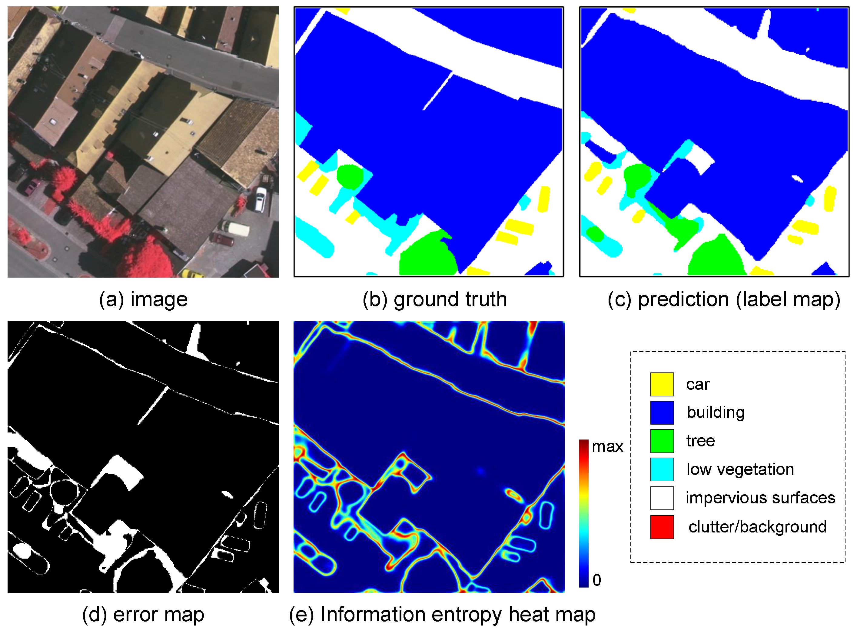
To tackle the above problems, we propose a gated convolutional neural network for the semantic segmentation in high-resolution images, called gated segmentation network (GSN). When combining two feature maps, we introduce an input gate to adaptively decide whether to keep the corresponding information. Generally speaking, our goal is to import extra low-level information at the positions where the pixel labels are difficult to infer by only using the upper layer feature maps. Meanwhile, we prevent low-level information from being imported into the combined features if the pixel labels have already been determined. This is because over-segmentation may arise if we bring overmuch details. The gate mechanism is implemented by calculating the information entropy of the feature maps before the softmax layer (classifier). The generated entropy heat map has strong relationship with the label-error map, as shown in Figure 1d,e. We summarize our contributions as follows:
- A gated network architecture is proposed for adaptive information propagation among feature maps with different level. With this architecture, convolution layers propagate the selected information into the final features. In this way, local and contextual features work with each other for improving the segmentation accuracy.
- An entropy control layer is introduced to implement the gate. It is based on the observation that the information entropy of the feature maps before the classifier are closely related to the label-error map of the segmentation, as shown in Figure 1.
- A new deep learning pipeline for semantic segmentation is proposed. It effectively integrates local details and contextual information and can be trained via an end-to-end manner.
- The proposed method achieves state-of-the-art performance among all the published papers on the ISPRS 2D semantic labeling benchmark. Specifically, our method achieves a mean score of 88.7% on five categories (ranking 1st) and overall accuracy 90.3% (ranking 1st). It should be noted that these results are obtained using only RGB images with a single model, without Digital Surface Model (DSM) and model ensemble strategy.
The remainder of this paper is organized as follows: Section 2 presents the related work. In Section 3.2, we introduce the proposed GSN architecture. Section 4 validates our approach experimentally, followed the conclusions in Section 5.
2. Related Work
2.1. Deep Learning
In 2012, the AlexNet [16] won the ILSVRC contest, which is a key milestone in deep learning. Since then, DCNNs have got an explosive development. VGG [17], GoogLeNet [18], ResNet [19] have been proposed one after another. These frameworks are usually treated as feature extractor and play an import role in a wide range of computer vision tasks, such as object detection [20], semantic segmentation [21] and scene understanding [22], etc.
2.2. Semantic Segmentation in Remote Sensing
Semantic segmentation is a significant branch in computer vision. There are a considerable number of works focusing on the remote sensing imagery. Full reviews can be found in [23,24,25]. Generally, these methods can be roughly classified into the pixel-to-pixel and image-to-image segmentation. The pixel-to-pixel method determines a pixel’s label based on an image patch enclosing the target pixel. Then other pixels are classified using a sliding window approach [26,27]. With the development of deep learning on remote sensing images, image-to-image segmentation becomes the mainstream. Sherrah and Jamie [8] proposed a deep FCN with no down-sampling to infer a full-resolution label map. Their method employs the strategy of the dilated convolution in DeepLab [21], which uses dilated kernel to enlarge the size of convolution output at the expense of storage cost. Marmanis et al. [28] embedded boundary detection to the SegNet encoder-decoder architecture. The boundary detection significantly improves semantic segmentation performance with extra model complexity. Kampffmeyer et al. [29] focused on small object segmentation through measuring the uncertainty for DCNNs. This approach achieves high overall accuracy as well as good accuracy for small objects. For all the above methods, further improvements can be achieved by using Conditional Random Fields (CRF) [30,31] or additional data (e.g., Digital Surface Model).
2.3. Gate in Neural Networks
Long short-term memory (LSTM) [32] is a famous framework in the natural language and speech processing. Its success largely owes to the design of gate to control the message propagation. Recently, Dauphin et al. [33] introduced the gated convolutional networks to substitute LSTM for language modeling. A convolution layer followed by a sigmoid layer is treated as a gate unit. Similar to [33], GBD-Net [34] also uses convolution layers with the sigmoid non-linearity as gate unit. GBD-Net is designed for object detection. The gate units are used for passing information among features from different RoIs (region of interest). Through analysis of related literature, embedding gate in neural networks is a simple, yet effective way for both feature learning and feature fusion.
3. Method
This section starts with an important observation of DCNNs for semantic segmentation, which motivates us to design the gated segmentation network (GSN). Then we introduce the GSN architecture in detail, which largely improves the performance of semantic segmentation in remote sensing images.
3.1. Important Observation
When applying DCNNs for the semantic segmentation, the softmax (cross entropy) is usually used as the classifier for the given feature maps. The output of the softmax represents a probability distribution of each pixel over K different categories. With the estimated probabilities of pixel x, we can calculate the corresponding entropy with
where denotes expectation over all the K categories, and is the probability of pixel x belonging to category i.
We observe that the entropy heat map has strong relationship with the label-error map. As shown in Figure 1d,e, there is a strong possibility that the pixels of high entropy are wrong classified. Generally, entropy is a measure of the unpredictability of states [35]. When the entropy of pixel x is maximized, approximates an uniform probability distribution, indicating that the network is unable to classify this pixel by using only existing information. At these positions, extra information is needed to help the network to classify the pixels. On the contrary, when the network has a high confidence in the pixel label, the entropy will become lower. According to this consideration, when we combine low-level feature maps with high-level ones, the entropy heat map can be treated as a weight map of the low-level feature maps.
3.2. Gated Segmentation Network
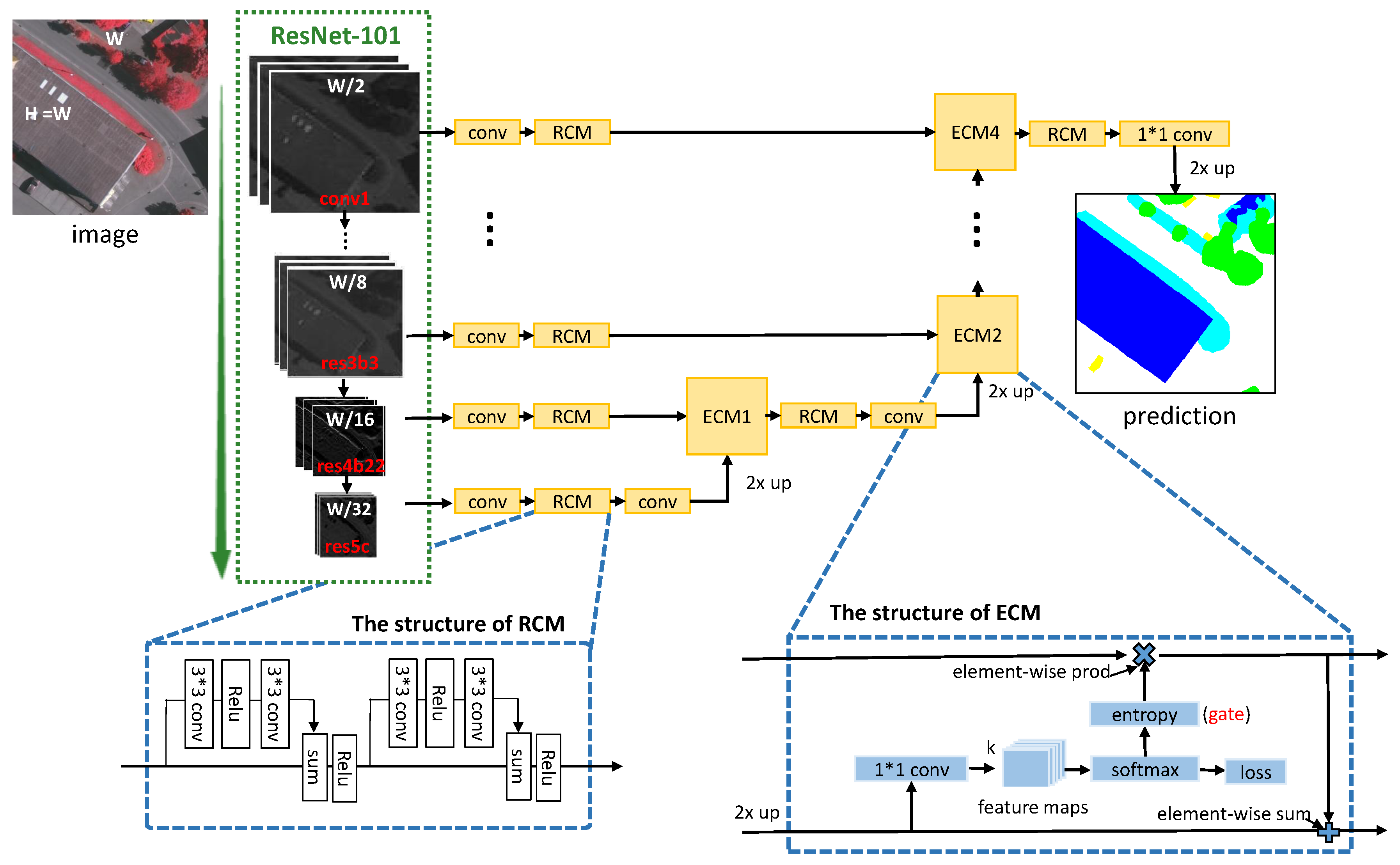
Based on the above observation, we propose a gated convolutional neural network for the semantic segmentation in high-resolution images. An overview of the GSN architecture is shown in Figure 2. Our architecture can be divided into two parts: encoder and decoder. In the encoder part, ResNet-101 is applied for feature extraction. In this process, we can get low-level feature maps containing detailed information from lower layers, as well as high-level feature maps containing high-level contextual information from upper layers. In the decoder part, we first use the high-level feature maps for semantic segmentation and get the entropy heat map. Then the generated entropy heat map is treated as the input weight (pixel-to-pixel) of the low-level feature maps when merged with high-level feature maps. A larger entropy value indicates higher uncertainty about the label of the pixel. Consequently, a higher adoption of the low-level feature maps is necessary. We repeat this operation until all the available low-level feature maps are combined. Additionally, residual convolution module is introduced as the basic processing unit before and after the merging process for better training the network. Finally, the combined feature maps containing both high- and low-level information are fed into the softmax layer to obtain the segmentation result. The details are described in the subsequent subsections.
3.2.1. Entropy Control Module
The bottom-right corner of Figure 2 shows the structure of the proposed entropy control module (ECM). It takes the feature maps (already up-sampled) and as input. The output is represented by , which combines contextual information and details from and respectively. This feature fusion process is implemented by a gate function, which can be summarized as follows:
where ⊗, ⊙ and ⊕ stands for the convolution operator, the element-wise product operator, and the element-wise sum operator respectively, and represents the convolutional kernel. As there are K categories in our work setting, the output of the convolutional layer will contain K channels, and each channel records the probabilities of pixels belonging to one of the K categories. In Equation (2), stands for the entropy calculator, which yields the entropy heat map by Equation (1).
Based on Equation (2), one can see that the designed gate is a binary function, which takes the entropy heat map and the low-level feature map as its inputs. Functionally, it is actually a feature selector on , which is guided by the entropy heat map that is originated from the high-level feature map . Beyond simply fusing the , in this way we build up a mechanism to select the features with their importance for classification. In practice, an entropy control layer is introduced to implement the gate. This layer is only used for calculating the entropy, thus it does not participate in the process of back-propagation.
For clarity, we take Figure 1e as an example to explain our design. Actually, the entropy heat map generated by offers very helpful information for classifying those pixels that are hard to be classified. As can be witnessed in Figure 1e, most of the high-entropy pixels appear on the object boundaries. Thus, with the gate operation, the information from lower layer will be passed and highly weighted into the final (see Equation (2)). In contrast, the entropy inside the objects is usually low. Sequentially, the information from lower layer at these positions (e.g., the chimney in the roof in Figure 1e) will be blocked. As a result, over-segmentation can be avoided.
3.2.2. Residual Convolution Module
Inspired by ResNet, residual convolution module (RCM) is introduced as the basic processing unit to ease the training of the network. As shown in the bottom-left corner of Figure 2, there is an identity mapping between the input and output of the module. In the forward propagation, input message can be delivered without loss, and network only needs to learn the residual mapping. In the backward propagation, gradient can be directly propagated from top to bottom, which can settle the problem of gradient vanishing. Compared with the residual blocks in ResNet, the RCM has two differences. First, we removed the convolutional layer. Compute reduction layers have been added at the begin of encoder. Numbers of feature channels are small in the decoder and compute reduction becomes unnecessary. Second, batch normalization layer [36] is removed. Given that the model size is large, we are limited to use small batch size to stay within the GPU memory capacity.
3.2.3. Model Optimization
In the field of neural networks, model optimization is driven by a loss function (also known as objective function). Once the loss function is defined, we can train the network by back-propagation errors [37] in conjunction with gradient descent. To train the proposed architecture, softmax loss function, i.e., cross entropy loss, is adopted. We have a main loss at the end of network and four auxiliary losses in four ECMs. For clarity, we only consider the main loss in the following analysis. Specifically, the softmax function is defined as:
where represents the parameters of the proposed GSN, B and P are the mini-batch size and number of pixels in each image respectively, is the indicator function, which takes 1 when and 0 otherwise, is the p-th pixel in the b-th batch and is the corresponding label, and the probability of pixel belonging to the k-th class is denoted by , which can be calculated by:
where is the j-th filter of the last conv layer, d is the feature dimension, are the rest parameters except the conv layer, and denotes the learned deep features.
To train the GSN in an end-to-end manner, the stochastic gradient descent (SGD) is adopted for the optimization. Thus, the derivatives of the loss to different convolutional layers need to be calculated with chain rule. Taking the conv layer as an example, the partial derivative of the loss with respect to is acquired by
We can get the partial derivative of loss with respect to the parameters in other layers by chain rule. In Algorithm 1, we summarize the learning steps with SGD.
| Algorithm 1 The training algorithm for the proposed GSN. |
| Input: Training data x, maximum iteration T. Initialize the parameters θ in convolutional layers, learning rate αt, learning rate policy ploy. Set the initialized iteration t ← 0. Output: The leanred parameter θ. 1: while do 2: . 3: Call network forward to compute the output and loss L. 4: Call network backward to compute the gradients . 5: Update the parameters by . 6: Updates the according to learning rate policy. 7: end while |
3.3. Implementation Details
[-5]We fine-tune the model weights of ResNet-101 pre-trained on Imagenet [38] to our GSN model. Five kinds of feature maps with different sizes (acquired from the outputs of branches in [“res5c”, “res4b22”, “res3b3”, “res2c”, “conv1”]) are prepared to be merged in the decoder part. The spatial sizes of these feature maps are [, , , , ] respectively, with input image . Dropout is applied after these feature maps with ratio 0.5 to avoid overfitting [39]. Moreover, we further add a convolutional (conv) layer after the dropout layer mainly to reduce the channels. The channels of the five branches are set to [256, 128, 128, 64, 64] respectively. Intuitively, similar conv layers should be applied before the up-sampled layers ( up), since the channels are different between these branches.
The proposed GSN is implemented with Caffe [40] on GPU (TITAN X). Our loss function is the sum of softmax loss, which comes from the final classification and four ECMs. Initial learning rate is 0.0004. We employ the “ploy” learning rate policy. Momentum and weight decay are set to 0.9 and 0.0005 respectively. The bath size is set to 1. The maximum iteration is 30 k. The total training time is about 24 h, and the average testing time of one image (600 × 600) is about 100 ms.
4. Experiments
4.1. Dataset
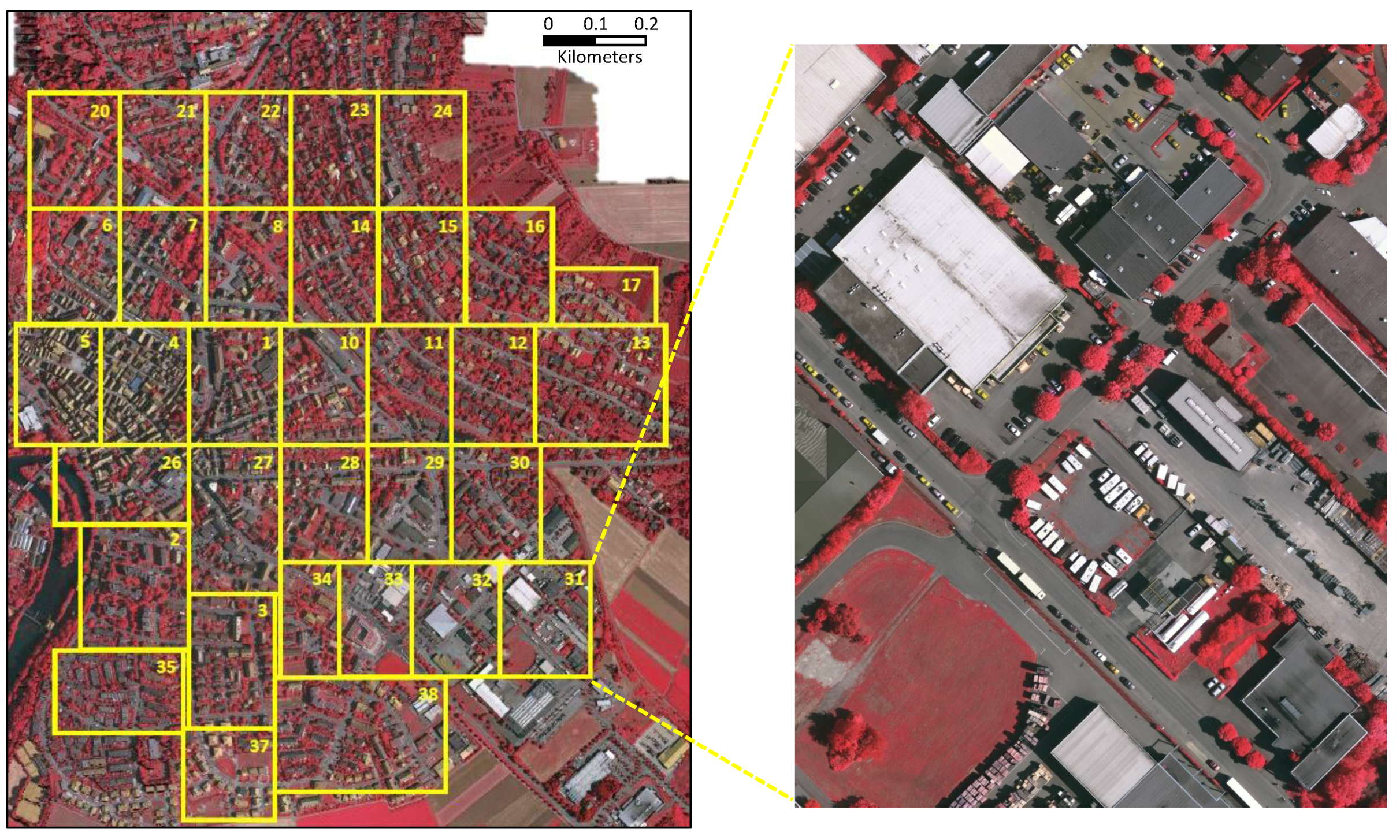
We evaluate the proposed method on the ISPRS 2D semantic labeling contest [41], which is an open benchmark dataset. The dataset contains 33 very high-resolution true orthophoto (TOP) tiles extracted from a large TOP mosaic as shown in Figure 3. Each tile contains around 2500 × 2000 pixels with a resolution of 9 cm. The dataset has been manually classified into six most common land cover classes, as shown in Figure 1. The clutter class includes water bodies and other objects that look very different from other objects (e.g., containers, tennis courts, swimming pools). As previously done in other methods, the class of clutter is not included in the experiments, as the pixels of the clutter class only account for 0.88% of the total image pixels. ISPRS only provides 16 labeled images for training, while the remaining 17 tiles are unreleased and used for the evaluation of submitted results by the benchmark organizers. Following other methods, 4 tiles (image numbers 5, 7, 23, 30) are removed from the training set as a validation set. Experimental results are reported on the validation set if not specified.
Dataset augmentation: The 16 training tiles are first rotated 90 and 180 degrees. Then, we sample 600 × 600 patches from original images with stride (300 pixels) to avoid the insufficiency of GPU memory. Moreover, we also randomly process the input images at the training stage with the following one or combined operations: mirror, rotated between −10 and 10 degrees, resize by a factor between 0.5 and 1.5, and Gaussian blur.
Evaluation: According to the benchmark rules, score and overall accuracy are used to assess the quantitative performance. score is calculated by:
where
where , and are true positive, false positive and false negative respectively. These values can be calculated by pixel-based confusion matrices per tile, or an accumulated confusion matrix. Overall accuracy is the normalization of the trace from the confusion matrix.
4.2. Model Analysis
For the sake of convenient comparison, we use the result of GSN without entropy control module (ECM) as our baseline, which uses the sum operation to merge the feature maps. As shown in Table 1, the model with ECM outperforms the baseline by a significant margin. This proves that the ECM can effectively control information propagation and integrate features of different level effectively. One can also see that the auxiliary loss in ECM is helpful for model optimization (GSN vs. GSN_noL). The auxiliary loss forces the network to learn accurate contextual feature before merging lower feature maps with high-spatial. Moreover, we notice from the confusion matrix that the low_veg and car are more likely to be classified into tree and imp_suf respectively. This motivates us to slightly increase the weights of low_veg to 1.1 and car to 1.2 in the loss function without accurate selection (GSN vs. GSN_w). Finally, we have reported the result with sliding window overlap and multi-scale input, i.e., GSN_w_mc. Averaging predictions on the overlap regions reduce the risk of error classification, since the borders of one patch is difficult to predict due to the lack of context.
4.3. Comparisons with Related Methods
To show the effectiveness of the proposed method, we have performed comparisons against a number of state-of-the-art semantic segmentation methods, as listed in Table 2. Deeplab-v2 [21] and RefineNet [15] are the versions with ResNet-101 as their encoder. In particular, we re-implement the RefineNet with Caffe, since the released code is built on MatConvNet [42]. We can see that GSN significantly outperforms other methods on both overall accuracy and mean score. Notably, our approach outperforms the RefineNet, within which the feature map merging is implemented by the sum operation. The comparison indicates that the promising performance of GSN can be ascribed to the ECM, which selects low-level information in feature fusion.
4.4. Model Visualization
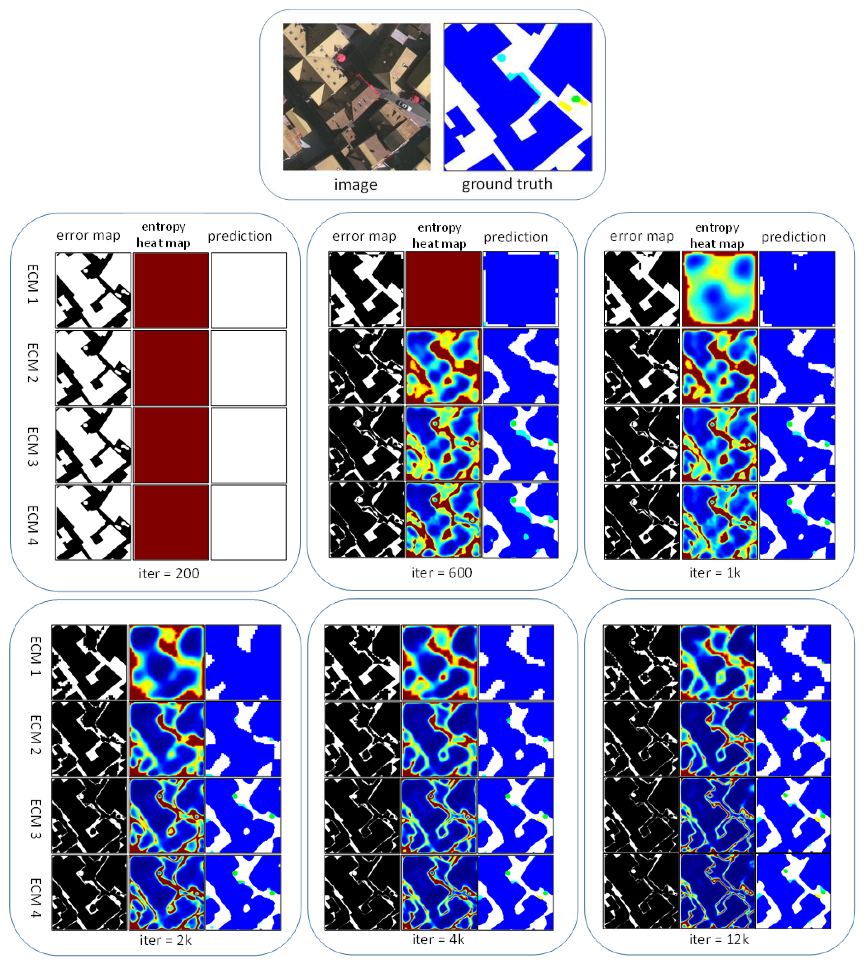
To understand GSN better, we have also carried out feature map visualization to examine how entropy gate affects the final performance. Four entropy control modules are embedded in GSN to merge the five kinds of feature maps with different resolutions. In this section, we visualize the entropy heat map, error map and prediction in each ECM.
At each iteration , the prediction will be more fine-grained by merging larger resolution feature maps (ECM 1 → ECM 4). An illustration is provided in Figure 4. In ECM 1, we only get a coarse label map, since only the smallest resolution maps are available. Successively merging features from lower layers, we can refine the coarse label map. This is consistent with the analysis of upper-layer feature maps containing more contextual information, and lower-layer feature maps containing more details.
In addition, we also visualize the three kinds of maps at different iterations while training the model. At the beginning, the entropy heat maps of four ECMs are almost the same, i.e., red images. It shows that the value of entropy is very high at the beginning, and thus all the gates are at the fully opened state. At this moment, the network has not learned the discriminative features and needs additional information to determine the pixels’ labels. As the training proceeds, GSN learns more discriminative features and starts to close the gates at some positions, as shown in 600 or 1 k iterations. Towards the end of the training, we acquire a more satisfying prediction. As can be seen in Figure 4, the positions of high entropy values (similar to error map) almost appear on the boundaries, whose width is very thin. All the above observations once again demonstrate the effectiveness of the proposed ECM.
4.5. ISPRS Benchmark Testing Results
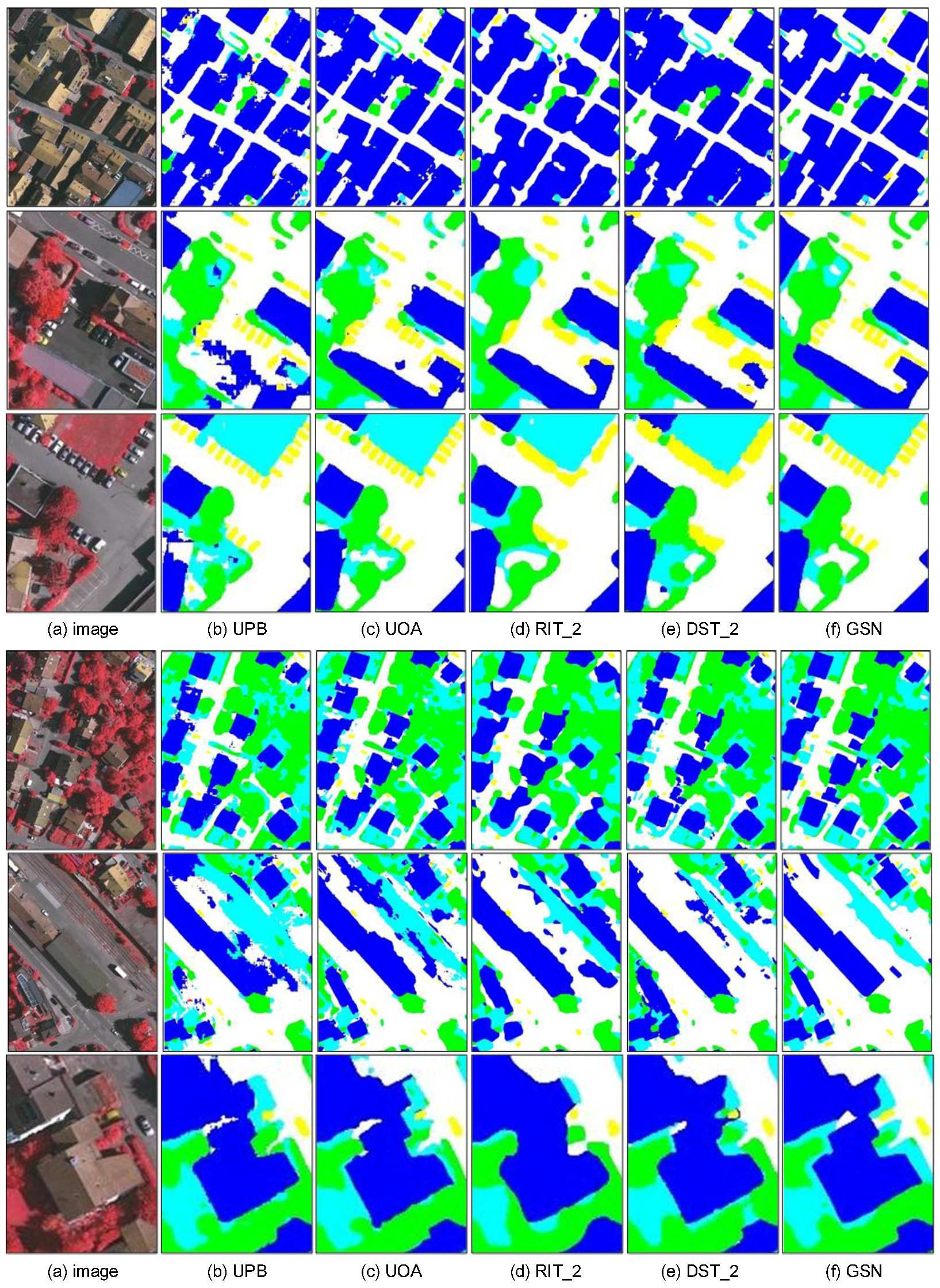
We submitted the results on the unlabelled test images to ISPRS organizers for evaluation. As shown in Table 3, GSN ranks 1st both in mean score and overall accuracy, compared with all the other published works. Visual performance among related methods is shown in Figure 5. It should be noted that we only use the RGB source images. Neither the additional DSM images offered by ISPRS nor the CRF for post-processing is used in the proposed method, both of which can further improve the performance as described in these compared methods. This is based on the following two considerations. First, we want to sufficiently mine the information contained in RGB images, which will eliminate the need to acquire DSM data. Second, the operation of CRF is time-consuming. Therefore, we manage to build a fast and simple architecture for sematic segmentation in high-resolution remote sensing images. In addition, according to the evaluation of ISPRS, the boundaries of objects in testing labeled images are eroded by a circular disc of 3 pixel radius. Those eroded areas are ignored during evaluation in order to reduce the impact of uncertain border definitions. Thus the performance on testing set is slightly better than that on validation set.
4.6. Failed Attempts
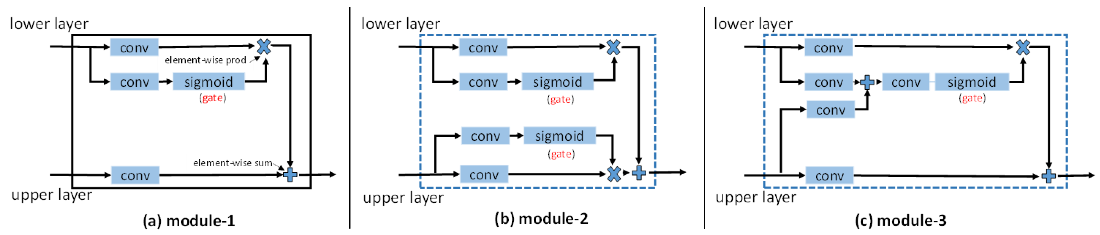
Before creating entropy control module, many failed attempts have been made to find an effective way for feature fusion. Motivated by [33,34], we once tried to create the gate by using convolutional layer followed by sigmoid non-linearity, which make the information propagation rate in the range of (0, 1). Three modules have been designed based on this idea. As shown in Figure 6, we have attempted to add the gate in the output of the lower or upper layer. In the third module, gate on the output of lower layer is created by the combination of lower and upper layers output. However, as shown in Table 4, these modules are less effective than we expected. It is because they can not learn the right open (or closed) state due to the lack of supervised information. One may consider adding auxiliary losses in these modules to guide learning. However it is not feasible. Sigmoid is just an activation layer that has nothing to do with the label-error map. There is no supervised information to guide the network training. Thus we cannot get the right gate states. In contrast, entropy has a strong relationship with the label-error map, which is the supervised information for controlling the gate states. This is the reason why ECM can effectively select features and improve the segmentation performance.
5. Conclusions
In this paper, a gated convolutional neural network was proposed for the semantic segmentation in high-resolution aerial images. We introduced entropy control module (ECM) to guide the message passing between feature maps with different resolutions. The ECM can effectively help for integrating contextual information from the upper layers and details from the lower layers. Extensive experiments on the ISPRS dataset demonstrate that the proposed method achieve clear promising gains compared with the state-of-the art methods. Our approach has the potential to perform better. Actually, the pixels in a certain region are interrelated. However, we calculate the entropy map (gate) pixel-to-pixel, which ignores the relationships between surrounding pixels. In the future work, we will try to incorporate gaussian smoothing into the entropy map to further improve the performance. In addition, we will also try to apply GSN to other fine-grained semantic segmentation tasks.
Acknowledgments
This work was supported in part by the National Natural Science Foundation of China under Grants 91646207, 91338202, 91438105, and the Beijing Natural Science Foundation under Grant 4162064.
Author Contributions
Hongzhen Wang and Shiming Xiang designed the deep learning model; Hongzhen Wang performed the experiments; Ying Wang analyzed the solution to the model; Shiming Xiang and Chunhong Pan analyzed the data; Qian Zhang contributed the analysis tools and comparative methods; Hongzhen Wang and Chunhong Pan wrote the paper.
Conflicts of Interest
The authors declare no conflict of interest.
References
- Wang, Q.; Lin, J.; Yuan, Y. Salient band selection for hyperspectral image classification via manifold ranking. IEEE Trans. Neural Netw. Learn. Syst. 2016, 27, 1279–1289. [Google Scholar] [CrossRef] [PubMed]
- Cheng, G.; Zhu, F.; Xiang, S.; Wang, Y.; Pan, C. Accurate urban road centerline extraction from VHR imagery via multiscale segmentation and tensor voting. Neurocomputing 2016, 205, 407–420. [Google Scholar] [CrossRef]
- Yuan, Y.; Lin, J.; Wang, Q. Dual-clustering-based hyperspectral band selection by contextual analysis. IEEE Trans. Geosci. Remote Sens. 2016, 54, 1431–1445. [Google Scholar] [CrossRef]
- Matikainen, L.; Karila, K. egment-based land cover mapping of a suburban area—Comparison of high-resolution remotely sensed datasets using classification trees and test field points. Remote Sens. 2011, 3, 1777–1804. [Google Scholar] [CrossRef]
- Tang, Y.; Zhang, L. Urban change analysis with multi-sensor multispectral imagery. Remote Sens. 2017, 9, 252. [Google Scholar] [CrossRef]
- Yuan, Y.; Lin, J.; Wang, Q. Hyperspectral image classification via multitask joint sparse representation and stepwise MRF optimization. IEEE Trans. Cybern. 2016, 46, 2966–2977. [Google Scholar] [CrossRef] [PubMed]
- Zhang, Q.; Seto, K.C. Mapping urbanization dynamics at regional and global scales using multi-temporal DMSP/OLS nighttime light data. Remote Sens. Environ. 2011, 115, 2320–2329. [Google Scholar] [CrossRef]
- Sherrah, J. Fully convolutional networks for dense semantic labelling of highresolution aerial imagery. arXiv 2016. [Google Scholar]
- Girshick, R. Fast r-cnn. In Proceedings of the IEEE International Conference on Computer Vision, Santiago, Chile, 13–16 December 2015; pp. 1440–1448. [Google Scholar]
- Goodfellow, I.; Pouget-Abadie, J.; Mirza, M.; Xu, B.; Warde-Farley, D.; Ozair, S.; Courville, A.; Bengio, Y. Generative adversarial nets. In Proceedings of the Advances in Neural Information Processing Systems, Montreal, QC, Canada, 8–13 December 2014; pp. 2672–2680. [Google Scholar]
- Yang, S.; Luo, P.; Loy, C.C.; Tang, X. From facial parts responses to face detection: A deep learning approach. In Proceedings of the IEEE International Conference on Computer Vision, Santiago, Chile, 13–16 December 2015; pp. 3676–3684. [Google Scholar]
- Long, J.; Shelhamer, E.; Darrell, T. Fully convolutional networks for semantic segmentation. IEEE Trans. Pattern Anal. Mach. Intell. 2015, 79, 1337–1342. [Google Scholar]
- Ronneberger, O.; Fischer, P.; Brox, T. U-net: Convolutional networks for biomedical image segmentation. In Proceedings of the International Conference on Medical Image Computing and Computer-Assisted Intervention, Munich, Germany, 5–9 October 2015; Springer: Cham, Switzerland, 2015; pp. 234–241. [Google Scholar]
- Badrinarayanan, V.; Kendall, A.; Cipolla, R. Segnet: A deep convolutional encoder-decoder architecture for image segmentation. arXiv 2015. [Google Scholar]
- Lin, G.; Milan, A.; Shen, C.; Reid, I. RefineNet: Multi-path refinement networks with identity mappings for high-resolution semantic segmentation. arXiv 2016. [Google Scholar]
- Krizhevsky, A.; Sutskever, I.; Hinton, G.E. Imagenet classification with deep convolutional neural networks. In Proceedings of the Advances in Neural Information Processing Systems, Lake Tahoe, NV, USA, 3–6 December 2012; pp. 1097–1105. [Google Scholar]
- Simonyan, K.; Zisserman, A. Very deep convolutional networks for large-scale image recognition. arXiv 2014. [Google Scholar]
- Szegedy, C.; Liu, W.; Jia, Y.; Sermanet, P.; Reed, S.; Anguelov, D.; Erhan, D.; Vanhoucke, V.; Rabinovich, A. Going deeper with convolutions. In Proceedings of the IEEE Conference on Computer Vision and Pattern Recognition, Boston, MA, USA, 7–12 June 2015; pp. 1–9. [Google Scholar]
- He, K.; Zhang, X.; Ren, S.; Sun, J. Deep residual learning for image recognition. In Proceedings of the IEEE Conference on Computer Vision and Pattern Recognition, Seattle, WA, USA, 27–30 June 2016; pp. 770–778. [Google Scholar]
- Ren, S.; He, K.; Girshick, R.; Sun, J. Faster r-cnn: Towards real-time object detection with region proposal networks. In Proceedings of the Advances in Neural Information Processing Systems, Montreal, QC, Canada, 7–12 December 2015; pp. 91–99. [Google Scholar]
- Chen, L.C.; Papandreou, G.; Kokkinos, I.; Murphy, K.; Yuille, A.L. Deeplab: Semantic image segmentation with deep convolutional nets, atrous convolution, and fully connected crfs. arXiv 2016. [Google Scholar] [CrossRef] [PubMed]
- Zhou, B.; Khosla, A.; Lapedriza, A.; Oliva, A.; Torralba, A. Learning deep features for discriminative localization. In Proceedings of the IEEE Conference on Computer Vision and Pattern Recognition, Seattle, WA, USA, 27–30 June 2016; pp. 2921–2929. [Google Scholar]
- Ghamisi, P.; Dalla Mura, M.; Benediktsson, J.A. A survey on spectral–spatial classification techniques based on attribute profiles. IEEE Trans. Geosci. Remote Sens. 2015, 53, 2335–2353. [Google Scholar] [CrossRef]
- Bruzzone, L.; Demir, B. A review of modern approaches to classification of remote sensing data. In Land Use and Land Cover Mapping in Europe; Springer: Dordrecht, The Netherlands, 2014; pp. 127–143. [Google Scholar]
- Zhang, L.; Zhang, L.; Du, B. Deep learning for remote sensing data: A technical tutorial on the state of the art. IEEE Geosci. Remote Sens. Mag. 2016, 4, 22–40. [Google Scholar] [CrossRef]
- Paisitkriangkrai, S.; Sherrah, J.; Janney, P.; van-Den Hengel, A. Effective semantic pixel labelling with convolutional networks and Conditional Random Fields. In Proceedings of the IEEE Conference on Computer Vision and Pattern Recognition Workshops, Boston, MA, USA, 7–12 June 2015; pp. 36–43. [Google Scholar]
- Audebert, N.; Le Saux, B.; Lefevre, S. How useful is region-based classification of remote sensing images in a deep learning framework? In Proceedings of the IEEE Conference on Geoscience and Remote Sensing Symposium, Beijing, China, 10–15 July 2016; pp. 5091–5094. [Google Scholar]
- Marmanis, D.; Schindler, K.; Wegner, J.D.; Galliani, S.; Datcu, M.; Stilla, U. Classification with an edge: Improving semantic image segmentation with boundary detection. arXiv 2016. [Google Scholar]
- Kampffmeyer, M.; Salberg, A.B.; Jenssen, R. Semantic segmentation of small objects and modeling of uncertainty in urban remote sensing images using deep convolutional neural networks. In Proceedings of the IEEE Conference on Computer Vision and Pattern Recognition Workshops, Seattle, WA, USA, 27–30 June 2016; pp. 1–9. [Google Scholar]
- Arnab, A.; Jayasumana, S.; Zheng, S.; Torr, P.H. Higher order conditional random fields in deep neural networks. In Proceedings of the European Conference on Computer Vision, Amsterdam, The Netherlands, 8–16 October 2016; Springer: Cham, Switzerland, 2016; pp. 524–540. [Google Scholar]
- Zheng, S.; Jayasumana, S.; Romera-Paredes, B.; Vineet, V.; Su, Z.; Du, D.; Huang, C.; Torr, P.H. Conditional random fields as recurrent neural networks. In Proceedings of the IEEE Conference on International Conference on Computer Vision, Los Alamitos, CA, USA, 7–13 December 2015; pp. 1529–1537. [Google Scholar]
- Hochreiter, S.; Schmidhuber, J. Long short-term memory. Neural Comput. 1997, 9, 1735–1780. [Google Scholar] [CrossRef] [PubMed]
- Dauphin, Y.N.; Fan, A.; Auli, M.; Grangier, D. Language modeling with gated convolutional networks. arXiv 2016. [Google Scholar]
- Zeng, X.; Ouyang, W.; Yan, J.; Li, H.; Xiao, T.; Wang, K.; Liu, Y.; Zhou, Y.; Yang, B.; Wang, Z.; et al. Crafting GBD-Net for Object Detection. arXiv 2016. [Google Scholar]
- Shannon, C.E. A mathematical theory of communication. Bell Syst. Tech. J. 1948, 5, 3–55. [Google Scholar]
- Ioffe, S.; Szegedy, C. Batch normalization: Accelerating deep network training by reducing internal covariate shift. arXiv 2015. [Google Scholar]
- Rumelhart, D.E.; Hinton, G.E.; Williams, R.J. Learning representations by back-propagating errors. Nature 1986, 323, 533–536. [Google Scholar] [CrossRef]
- Russakovsky, O.; Deng, J.; Su, H.; Krause, J.; Satheesh, S.; Ma, S.; Huang, Z.; Karpathy, A.; Khosla, A.; Bernstein, M. ImageNet large scale visual recognition challenge. Int. J. Comput. Vis. 2015, 115, 211–252. [Google Scholar] [CrossRef]
- Hinton, G.E.; Srivastava, N.; Krizhevsky, A.; Sutskever, I.; Salakhutdinov, R.R. Improving neural networks by preventing co-adaptation of feature detectors. Comput. Sci. 2012, 3, 212–223. [Google Scholar]
- Jia, Y.; Shelhamer, E.; Donahue, J.; Karayev, S.; Long, J.; Girshick, R.; Guadarrama, S.; Darrell, T. Caffe: Convolutional architecture for fast feature embedding. arXiv 2014, 675–678. [Google Scholar]
- International Society for Photogrammetry and Remote Sensing (ISPRS). 2D Semantic Labeling Contest. Available online: http://www2.isprs.org/commissions/comm3/wg4/semantic-labeling.html (accessed on 1 April 2015).
- Vedaldi, A.; Lenc, K. Matconvnet: Convolutional neural networks for matlab. In Proceedings of the 23rd ACM international conference on Multimedia, Brisbane, Australia, 26–30 October 2015; 2015; pp. 689–692. [Google Scholar]
- Marcu, A.; Leordeanu, M. Dual local-global contextual pathways for recognition in aerial imagery. arXiv 2016. [Google Scholar]
- Tschannen, M.; Cavigelli, L.; Mentzer, F.; Wiatowski, T.; Benini, L. Deep structured features for semantic segmentation. arXiv 2016. [Google Scholar]
- Lin, G.; Shen, C.; van den Hengel, A.; Reid, I. Efficient piecewise training of deep structured models for semantic segmentation. In Proceedings of the IEEE Conference on Computer Vision and Pattern Recognition, Seattle, WA, USA, 27–30 June 2016; pp. 3194–3203. [Google Scholar]
- Piramanayagam, S.; Schwartzkopf, W.; Koehler, F.; Saber, E. Classification of remote sensed images using random forests and deep learning framework. In Proceedings of the SPIE Remote Sensing; International Society for Optics and Photonics: Edinburgh, UK, 2016; p. 100040L. [Google Scholar]
- Audebert, N.; Saux, B.L.; Lefèvre, S. Semantic segmentation of earth observation data using multimodal and multi-scale deep networks. arXiv 2016. [Google Scholar]
Figure 1.
The strong relationship between segmentation error label map with entropy heat map. (a) Input image; (b) Segmentation reference map; (c) Predicted label map; (d) Error map with white pixels indicating wrongly classified pixels; (e) Corresponding entropy heat map.
Figure 1.
The strong relationship between segmentation error label map with entropy heat map. (a) Input image; (b) Segmentation reference map; (c) Predicted label map; (d) Error map with white pixels indicating wrongly classified pixels; (e) Corresponding entropy heat map.

Figure 2.
The overview of our gated segmentation network. In the encoder part, we use ResNet-101 as the feature extractor. Then the Entropy Control Module (ECM) are proposed for feature fusion in decoder. In addition, we design the Residual Convolution Module (RCM) as a basic processing unit. The details of RCM and ECM are shown in the dashed boxes.

Figure 3.
Overview of the ISPRS 2D Vaihingen Labeling dataset. There are 33 tiles. Numbers in the figure refer to the individual tile flag.
Figure 3.
Overview of the ISPRS 2D Vaihingen Labeling dataset. There are 33 tiles. Numbers in the figure refer to the individual tile flag.

Figure 4.
Model visualization. We show the error maps, entropy heat maps, and predictions at different iterations in the training procedure. Four rows at each iteration block correspond to four ECMs, which are used to merge five kinds of feature maps with different resolutions.
Figure 4.
Model visualization. We show the error maps, entropy heat maps, and predictions at different iterations in the training procedure. Four rows at each iteration block correspond to four ECMs, which are used to merge five kinds of feature maps with different resolutions.

Figure 5.
Visual comparisons between GSN and other related methods on ISPRS test set. Images come from the website of ISPRS 2D Semantic Labeling Contest.
Figure 5.
Visual comparisons between GSN and other related methods on ISPRS test set. Images come from the website of ISPRS 2D Semantic Labeling Contest.

Figure 6.
Three failure modules. (a) Placing gate on the output of lower layer; (b) Placing gate both on the output of lower layer and upper layers; (c) Gate on the output of lower layer is created by the combination of lower and upper layers output.
Figure 6.
Three failure modules. (a) Placing gate on the output of lower layer; (b) Placing gate both on the output of lower layer and upper layers; (c) Gate on the output of lower layer is created by the combination of lower and upper layers output.

Table 1.
The scores of 5 categories on the validation set. GSN_noL represents that the auxiliary loss in ECM does not participate in the back propagation of the network. GSN_w is the version that assigns different weights to different classes in the loss function. GSN_w_mc represents we test GSN with sliding window overlap and multi-scale input.
| Method | Imp Surf | Building | Low_veg | Tree | Car | Overall Accuracy | Mean Score |
|---|---|---|---|---|---|---|---|
| baseline | 87.6% | 93.2% | 73.3% | 86.9% | 54.1% | 86.1% | 79.0% |
| GSN | 89.2% | 94.5% | 74.9% | 87.5% | 79.8% | 87.9% | 85.2% |
| GSN_noL | 89.1% | 94.3% | 74.7% | 87.4% | 78.7% | 87.8% | 84.8% |
| GSN_w | 89.5% | 94.4% | 75.9% | 87.8% | 80.9% | 88.3% | 85.7% |
| GSN_w_mc | 90.2% | 94.8% | 76.9% | 88.3% | 82.3% | 88.9% | 86.5% |
Table 2.
Comparisons between our proposed GSN with mainstream models.
| Method | Imp Surf | Building | Low_veg | Tree | Car | Overall Accuracy | Mean Score |
|---|---|---|---|---|---|---|---|
| FCN-8s [12] | 87.1% | 91.8% | 75.2% | 86.1% | 63.8% | 85.9% | 80.8% |
| SegNet [14] | 82.7% | 89.1% | 66.3% | 83.9% | 55.7% | 82.1% | 75.5% |
| Deeplab-v2 [21] | 88.5% | 93.5% | 73.9% | 86.9% | 84.7% | 86.9% | 83.5% |
| RefineNet [15] | 88.1% | 93.3% | 74.0% | 87.1% | 65.1% | 86.7% | 81.5% |
| GSN | 89.2% | 94.5% | 74.9% | 87.5% | 79.8% | 87.9% | 85.2% |
Table 3.
Quantitative comparisons between our method and other related methods (already published) on ISPRS test set.
Table 3.
Quantitative comparisons between our method and other related methods (already published) on ISPRS test set.
| Method | Imp Surf | Building | Low_veg | Tree | Car | Overall Accuracy | Mean Score |
|---|---|---|---|---|---|---|---|
| UPB [43] | 87.5% | 89.3% | 77.3% | 85.8% | 77.1% | 85.1% | 83.4% |
| ETH_C [44] | 87.2% | 92.0% | 77.5% | 87.1% | 54.5% | 85.9% | 79.7% |
| UOA [45] | 89.8% | 92.1% | 80.4% | 88.2% | 82.0% | 87.6% | 86.5% |
| ADL_3 [26] | 89.5% | 93.2% | 82.3% | 88.2% | 63.3% | 88.0% | 83.3% |
| RIT_2 [46] | 90.0% | 92.6% | 81.4% | 88.4% | 61.1% | 88.0% | 82.7% |
| DST_2 [8] | 90.5% | 93.7% | 83.4% | 89.2% | 72.6% | 89.1% | 85.9% |
| ONE_7 [47] | 91.0% | 94.5% | 84.4% | 89.9% | 77.8% | 89.8% | 87.5% |
| DLR_9 [28] | 92.4% | 95.2% | 83.9% | 89.9% | 81.2% | 90.3% | 88.5% |
| GSN | 92.2% | 95.1% | 83.7% | 89.9% | 82.4% | 90.3% | 88.7% |
Table 4.
Performance of the failure models.
| Model_1 | Model_2 | Model_3 | GSN | |
|---|---|---|---|---|
| overall accuracy | 83.4% | 60.0% | 82.2% | 86.1% |
| mean score | 75.3% | 57.3% | 74.8% | 79.0% |
© 2017 by the authors. Licensee MDPI, Basel, Switzerland. This article is an open access article distributed under the terms and conditions of the Creative Commons Attribution (CC BY) license (http://creativecommons.org/licenses/by/4.0/).
Share and Cite
MDPI and ACS Style
Wang, H.; Wang, Y.; Zhang, Q.; Xiang, S.; Pan, C. Gated Convolutional Neural Network for Semantic Segmentation in High-Resolution Images. Remote Sens. 2017, 9, 446. https://doi.org/10.3390/rs9050446
AMA Style
Wang H, Wang Y, Zhang Q, Xiang S, Pan C. Gated Convolutional Neural Network for Semantic Segmentation in High-Resolution Images. Remote Sensing. 2017; 9(5):446. https://doi.org/10.3390/rs9050446
Chicago/Turabian StyleWang, Hongzhen, Ying Wang, Qian Zhang, Shiming Xiang, and Chunhong Pan. 2017. "Gated Convolutional Neural Network for Semantic Segmentation in High-Resolution Images" Remote Sensing 9, no. 5: 446. https://doi.org/10.3390/rs9050446
Note that from the first issue of 2016, this journal uses article numbers instead of page numbers. See further details here.